Self-annihilation of the neutralino dark matter into two photons or a $Z$ and a photon in the MSSM.

F. Boudjema¹⁾, A. Semenov²⁾ and D. Temes¹⁾

1) LAPTH^†, B.P.110, Annecy-le-Vieux F-74941, France

2) Joint Institute of Nuclear Research, JINR, 141980 Dubna, Russia

Abstract

We revisit the one-loop calculation of the annihilation of a pair of the lightest neutralinos into a pair of photons, a pair of gluons and also a $Z$ photon final state. For the latter we have identified a new contribution that may not always be negligible. For all three processes we have conducted a tuned comparison with previous calculations for some characteristic scenarios. The approach to the very heavy higgsino and wino is studied and we argue how the full one-loop calculation should be matched into a more complete treatment that was presented recently for these extreme regimes. We also give a short description of the code that we exploited for the automatic calculation of one-loop cross sections in the MSSM that could apply both for observables at the colliders and for astrophysics or relic density calculations. In particular the automatic treatment of zero Gram determinants which appear in the latter applications is outlined. We also point out how generalised non-linear gauge fixing constraints can be exploited.

LAPTH-1106/05

^†UMR 5108 du CNRS, associée à l’Université de Savoie.

1 Introduction

We now have overwhelming evidence that ordinary matter accounts for a minute portion of what constitutes the Universe at large. Most impressive is the confirmation from the very recent WMAP data[1]. Very interestingly, many extensions of the standard model whose primary aim was related to the Higgs sector and the mechanism of symmetry breaking do provide a good dark matter candidate. Very soon, with the energy frontier that will open up at the LHC, intense searches for this new physics with its associated dark matter candidate will be pursued in earnest.
Meanwhile, many astroparticle experiments are going on, and will be improved by the time the LHC runs, to detect dark matter particles. The problem, either for direct or indirect detection of dark matter outside the colliders, is that we do not control many astrophysical parameters. For indirect detection which is the result of the annihilation of a dark matter pair in, say, the galactic halo of our galaxy, the photon signal is cleaner than that of the charged positron and antiproton that are considered as sources of exotic cosmic rays. The photon will point back to the source while the antiproton flux suffers from uncertainties due to the propagation. Of course in both cases one still has to rely on a modelling of the dark matter profile since one needs to know the number density of the annihilating dark matter particles. A very distinctive signal though would be that of a “direct” annihilation into a monochromatic photon. In this case the spectrum will reveal a peak at an energy corresponding to the mass of the annihilating particles since the latter move at essentially zero relative velocity $v$. In the galactic halo $v/c\sim 10^{-3}$. Therefore, provided one has a detector with good energy resolution, the flux from the “direct” annihilation will clearly stand out above the (astrophysical) background or the diffuse contribution. The latter is due essentially to annihilation into quarks and $W$ which subsequently fragment and radiate/decay into photons. This contribution has a continuous featureless energy distribution which is only cut-off at a maximum energy corresponding to the mass of the dark matter particle. There are, and there will be, many powerful detectors to search for such photon signals, covering a wide range in energy from MeV to TeV. These are either ground based, like the atmospheric Cerenkov telescopes, ACT,(Cangaroo[2], HESS[3], MAGIC[4], VERITAS[5],..) or space borne telescopes (EGRET[7], AMS[6], the upcoming GLAST[8],..). Many see in some of the present data an excess that might be a sign for New Physics and dark matter annihilation but we should probably be cautious and await confirmation from other more precise detectors covering the same energy range. One should also improve on the theoretical predictions and a better understanding of the background and the astrophysical component that enter the calculation of the photon yield.
Our aim in this paper is to revisit the calculation of the “direct” self-annihilation into $\gamma\gamma$, $Z\gamma$ and $gg$ of the lightest supersymmetric particle (LSP). This is a neutralino that we will denote as $\tilde{\chi}^{0}_{1}$. There have been a few attempts of calculating the one-loop induced $\tilde{\chi}^{0}_{1}\tilde{\chi}^{0}_{1}\rightarrow\gamma\gamma$ before two complete calculations[9] settled the issue. These calculations have been made in the limit $v=0$ as is appropriate for dark matter annihilation in the halo. A very recent calculation[10] has also been made for this mode. Their results for $v=0$ agree in their most important features (higgsino limit, for example) with those of Refs [9], but as far as we are aware no systematic comparison has been performed. Much more important however is that there is, at the moment, only one calculation of $\tilde{\chi}^{0}_{1}\tilde{\chi}^{0}_{1}\rightarrow Z\gamma\;$[11] (performed at $v=0$) despite the fact that new features appear in this computation. These features, as we will see, can not be a mere generalisation of the $2\gamma$ final state. We will in this paper calculate both $\tilde{\chi}^{0}_{1}\tilde{\chi}^{0}_{1}\rightarrow\gamma\gamma\;$and $\tilde{\chi}^{0}_{1}\tilde{\chi}^{0}_{1}\rightarrow Z\gamma\;$for any velocity and make a tuned comparison with the existing codes for $v=0$, DarkSUSY[12] for $\tilde{\chi}^{0}_{1}\tilde{\chi}^{0}_{1}\rightarrow\gamma\gamma\;$and $\tilde{\chi}^{0}_{1}\tilde{\chi}^{0}_{1}\rightarrow Z\gamma\;$and PLATONdml for $\tilde{\chi}^{0}_{1}\tilde{\chi}^{0}_{1}\rightarrow\gamma\gamma\;$. In $\tilde{\chi}^{0}_{1}\tilde{\chi}^{0}_{1}\rightarrow Z\gamma\;$we have identified a new contribution not taken into account in[11]. We will also show some results for $v=0.5$ for both processes.
As a by-product we will also compute the self-annihilation into gluons: $\tilde{\chi}^{0}_{1}\tilde{\chi}^{0}_{1}\rightarrow gg\;$[13]. This can be derived from $\tilde{\chi}^{0}_{1}\tilde{\chi}^{0}_{1}\rightarrow\gamma\gamma\;$by only keeping the coloured particles and dealing properly with the colour structure. This process could contribute to, for example, the antiproton signal. We will see that our results for $\tilde{\chi}^{0}_{1}\tilde{\chi}^{0}_{1}\rightarrow gg\;$completely agree with those of DarkSUSY[12] and PLATONdmg[10] for $v=0$ and with PLATONgrel[10] for $v=0.5$.

As is known[9, 11], the largest contributions to $\tilde{\chi}^{0}_{1}\tilde{\chi}^{0}_{1}\rightarrow\gamma\gamma\;$and $\tilde{\chi}^{0}_{1}\tilde{\chi}^{0}_{1}\rightarrow Z\gamma\;$, especially for large neutralino masses, occur when the neutralino is a wino or a higgsino. As first pointed out in [9, 11] the cross section times the relative velocity, $\sigma v$, for both modes, tends to an asymptotic constant value that scales as $1/M_{W}^{2}$ for $v=0$ and large LSP mass. This result which breaks unitarity is due to the one-loop treatment of a “threshold” singularity that is nonetheless regulated by $M_{W}$. It has very recently been, admirably, shown[14] how to include the higher order corrections through a non-relativistic non-perturbative approach. The latter reveals the formation of bound states with zero binding energy that show up as sharp resonances that dramatically enhance the cross section for particular masses. We have therefore thought it worthwhile to study the one-loop derivation in these scenarios and see how one can match the non-perturbative regime. The reason we do this and the main reason we carry the calculation of $\tilde{\chi}^{0}_{1}\tilde{\chi}^{0}_{1}\rightarrow\gamma\gamma\;$and $\tilde{\chi}^{0}_{1}\tilde{\chi}^{0}_{1}\rightarrow Z\gamma\;$is that one needs a reliable code for the photon flux from self-annihilating neutralino LSP’s. These cross sections have been missing from micrOMEGAs[15] that we have been developing for a very accurate derivation of the relic density in supersymmetry and which is currently being adapted to direct and indirect detection. The present paper only deals with the cross section calculation, leaving aside the astrophysical issues to the implementation and exploitation within micrOMEGAs. See however Ref. [16] for a preliminary use of micrOMEGAs  to indirect detection using some of the results of this paper.
The results presented in this paper constitute some of the first applications of a code for the automatic computation of one-loop processes in supersymmetry relevant both for the colliders and astrophysics, such as the problem at hand. Most crucial for the latter is a careful treatment of the loop integrals since for these applications the use of general libraries is not appropriate leading to division by zero because of the appearance of vanishing Gram determinants in the reduction of the tensor integrals. We will show how to easily circumvent this problem.

2 Set-up of the automatic calculation

Even in the standard model, one-loop calculations of $2\rightarrow 2$ processes involve hundreds of diagrams and a hand calculation is practically impracticable. Efficient automatic codes for any generic $2\rightarrow 2$ processes, that have now been exploited for many $2\rightarrow 3$[17, 18] and even some $2\rightarrow 4$[19, 20] processes, are almost unavoidable for such calculations. For the electroweak theory these are the GRACE-loop[21] code and the package FormCalc[22] based on FeynArts[23] and LoopTools[24].
With its much larger particle content, far greater number of parameters and more complex structure, the need for an automatic code at one-loop for the minimal supersymmetric standard model is even more of a must. A few parts that are needed for such a code have been developed based on the package FeynArtsusy[25] but, as far as we know, no complete code exists or is, at least publicly, available. Grace-susy[26] is now also being developed at one-loop and many results exist[27]. One of the main difficulties that has to be tackled is the implementation of the model file, since this requires that one enters the thousands of vertices that define the Feynman rules. On the theory side a proper renormalisation scheme needs to be set up, which then means extending many of these rules to include counterterms. When this is done one can just use, or hope to use, the machinery developed for the SM, in particular the symbolic manipulation part and most importantly the loop integral routines and tensor reduction algorithms.
The calculations that we are reporting here are based on a new automatic tool that uses and adapts modules, many of which, but not all, are part of other codes. We will report on this approach elsewhere. Here we will be brief. In this application we combine LANHEP[28] (originally part of the package COMPHEP[29]) with the FormCalc package but with an extended and adapted LoopTools. LANHEP is a very powerful routine that automatically generates all the sets of Feynman rules of a given model, the latter being defined in a simple and compact format very similar to the canonical coordinate representation. Use of multiplets and the superpotential is built-in to minimize human error. The ghost Lagrangian is derived directly from the BRST transformations. The LANHEP module also allows to shift fields and parameters and thus generates counterterms most efficiently. Understandably the LANHEP output file must be in the format of the model file of the code it is interfaced with. In the case of FeynArts both the generic (Lorentz structure) and classes (particle content) files had to be given. Moreover because we use a non-linear gauge fixing condition[21], the FeynArts default generic file had to be extended.
This brings us to the issue of the gauge-fixing. We use a generalised non-linear gauge[30] adapted to the minimal supersymmetric model. The gauge fixing writes

$${\mathcal{L}}_{GF} = -\frac{1}{\xi_{W}}|(\partial_{\mu}-ie\tilde{\alpha}\gamma_{\mu}-igc_{W}\tilde{\beta}Z_{\mu})W^{\mu\,+}+\xi_{W}\frac{g}{2}(v+\tilde{\delta}h+\tilde{\omega}H+i\tilde{\kappa}\chi_{3})\chi^{+}|^{2}$$

$$-\frac{1}{2\xi_{Z}}(\partial.Z+\xi_{Z}\frac{g}{2c_{W}}(v+\tilde{\epsilon}h+\tilde{\gamma}H)\chi_{3})^{2}-\frac{1}{2\xi_{\gamma}}(\partial.\gamma)^{2}.$$

$h$ and $H$ are the CP-even physical Higgses, with $h$ denoting the lightest. $\gamma$ is the photon field and the masses of the charged and neutral weak bosons are related through $M_{W}=M_{Z}c_{W}$. The $\chi$’s are the Goldstone fields. The non-linear gauge fixing parameters are $\tilde{\alpha}$, $\tilde{\beta}$, $\tilde{\delta}$, $\tilde{\omega}$, $\tilde{\kappa}$, $\tilde{\epsilon}$ and $\tilde{\gamma}$. The $\xi$ are the usual Feynman parameters. In our implementation the latter are set to $\xi=1$ not only to avoid very large expressions due to the “longitudinal” modes of the gauge bosons but most importantly so that high rank tensors for the loop integrals are not needed. Gauge parameter independence which is a non trivial check on the result of the calculation can be made through the non-linear gauge fixing terms. In many instances a particular choice of the non-linear gauge parameter may prove much more judicious than another. For the case at hand, $\tilde{\alpha}=1$, preserves $U(1)_{\rm em}$ gauge invariance which explains the vanishing of the $W^{+}\chi^{-}\gamma$ vertex. This will prove crucial for the calculation of $\tilde{\chi}^{0}_{1}\tilde{\chi}^{0}_{1}\rightarrow Z\gamma\;$.
This brings us to the implementation of the loop integrals and their use in the most general application to radiative corrections in SUSY both for the colliders, for indirect detection and improvement of the relic density calculation beyond tree-level. In LoopTools[24] for example, the tensor loop integrals are reduced recursively to a set of scalar integrals by essentially following the Passarino-Veltman procedure[31]. The reduction involves solving a set of equations that brings in the inverse Gram determinant. Although for applications to the colliders the latter only vanishes for exceptional points in phase space, for the indirect detection calculation of tensor integrals involving annihilating LSP’s with small relative velocity $v$, the Gram determinant is of order $v^{2}$. Therefore it vanishes exactly for $v=0$ or can get extremely small slightly away from this value rendering the calculation highly instable. In the Appendix we show how we dealt with this problem in an automatic implementation. In a nut-shell, we have used a segmentation procedure based on the fact that when some momenta are dependent like what occurs with $v=0$, a $N$-point function writes as a sum of $N-1$ point functions. This also applies to the tensorial structures. This observation is not new (see for example[9, 11]) and has been used mostly in hand calculations. Some aspects of it may be remotely related to[33]. The scheme also allows an expansion away from exactly vanishing Gram determinants.

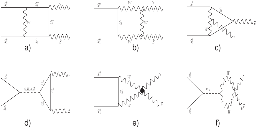
Figure 1: Typical classes of diagrams common to both $\tilde{\chi}^{0}_{1}\tilde{\chi}^{0}_{1}\rightarrow\gamma\gamma\;$and $\tilde{\chi}^{0}_{1}\tilde{\chi}^{0}_{1}\rightarrow Z\gamma\;$. For the former, the same “flavour” circulates in the loops and we do not have any mixing as in a) and d). Diagrams with Goldstone bosons are not shown. In the heavy wino and higgsino limit, a) is the dominant diagram. Diagrams d) and f) with $H,h$ exchange do not contribute for $v=0$.

A selection of diagrams that contribute to both $\tilde{\chi}^{0}_{1}\tilde{\chi}^{0}_{1}\rightarrow\gamma\gamma\;$and $\tilde{\chi}^{0}_{1}\tilde{\chi}^{0}_{1}\rightarrow Z\gamma\;$is shown in Fig. 1 (see also [9, 11]). Diagrams of type a) in Fig. 1 are particularly important in the large wino and higgsino limit. In this limit the LSP and the internal chargino are of almost equal mass. If the $W$ mass can be neglected this leads to a threshold singularity.

                   

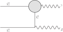
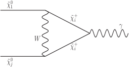
Figure 2: An additional class of diagrams describing the $\tilde{\chi}_{i}^{0}\rightarrow\tilde{\chi}^{0}_{1}\gamma$ transition that only appear in the case of $\tilde{\chi}^{0}_{1}\tilde{\chi}^{0}_{1}\rightarrow Z\gamma\;$. A representative of the blob is the virtual correction. The counterterm contribution is shown also.

Moving from $\tilde{\chi}^{0}_{1}\tilde{\chi}^{0}_{1}\rightarrow\gamma\gamma\;$to $\tilde{\chi}^{0}_{1}\tilde{\chi}^{0}_{1}\rightarrow Z\gamma\;$brings mixing effects in the loops. Most diagrams can be derived from $\tilde{\chi}^{0}_{1}\tilde{\chi}^{0}_{1}\rightarrow\gamma\gamma\;$. There is however an important class that is only present for $\tilde{\chi}^{0}_{1}\tilde{\chi}^{0}_{1}\rightarrow Z\gamma\;$as shown in Fig.2. This class of diagrams is missing in[11]. It corresponds to the insertion of the $\tilde{\chi}^{0}_{i}\rightarrow\tilde{\chi}^{0}_{1}\gamma$ transition. In a general gauge, the virtual transition would be gauge dependent and not ultraviolet finite. To remedy both these problems requires the $\tilde{\chi}^{0}_{i}\tilde{\chi}^{0}_{1}\gamma$ counterterm which is generated starting from the (tree-level) $\tilde{\chi}^{0}_{i}\tilde{\chi}^{0}_{1}Z$ vertex through a $Z-\gamma$ one-loop transition. It is well known that the latter is gauge dependent, see for example[21]. The counterterm requires the field normalisation $\delta Z_{Z\gamma}^{1/2}$[21]. This field renormalisation constant in fact also induces, like in the standard model, $(H,h)Z\gamma$ vertices not present at tree-level. This induced vertices are also needed for the class of diagrams shown in Fig. 1, in particular those with (H,h) exchange. The full set of counterterms for $\tilde{\chi}^{0}_{1}\tilde{\chi}^{0}_{1}\rightarrow Z\gamma\;$is in fact obtained from the tree-level $\tilde{\chi}^{0}_{1}\tilde{\chi}^{0}_{1}\rightarrow ZZ$, replacing a $Z$ by a photon and inserting the $\delta Z_{Z\gamma}^{1/2}$ renormalisation constant. However, it is known that this renormalisation constant vanishes for $\tilde{\alpha}=1$[21]. We have checked this property explicitly with our code. After this check has been made, $\tilde{\alpha}=1$ was set, since it considerably reduces the number of diagrams and most importantly allows to discard all the counterterm contributions. Further gauge parameter independence of the result for $\tilde{\chi}^{0}_{1}\tilde{\chi}^{0}_{1}\rightarrow Z\gamma\;$was checked by varying the other non-linear gauge parameters that enter the calculation, namely $\tilde{\beta},\tilde{\delta}$ and $\tilde{\omega}$. When discussing our results for $\tilde{\chi}^{0}_{1}\tilde{\chi}^{0}_{1}\rightarrow Z\gamma\;$we will weight the effect of the new class of diagrams shown in Fig. 2 against that of the full contribution, in doing so we will specialise to $\tilde{\alpha}=1$. As we will see these diagrams give a non negligible contribution especially for the Higgsino case.
The application to $\tilde{\chi}^{0}_{1}\tilde{\chi}^{0}_{1}\rightarrow gg\;$is rather straightforward. This process confirms that our code handles the colour summation correctly. Keeping only one flavour of quark with charge $Q_{f}$, $\tilde{\chi}^{0}_{1}\tilde{\chi}^{0}_{1}\rightarrow gg\;$can be derived from $\tilde{\chi}^{0}_{1}\tilde{\chi}^{0}_{1}\rightarrow\gamma\gamma\;$through $(N_{c}Q_{f}\alpha)^{2}\rightarrow 2\alpha_{s}^{2}$ ($N_{c}=3$ is the number of colours, $\alpha$ is the electromagnetic fine structure constant and $\alpha_{s}$ the QCD equivalent).

3 Results and comparisons

We first check that our results are ultraviolet finite by changing the numerical value of the parameter $1/\epsilon$ that controls a possible ultraviolet divergence. $\epsilon=4-n$, where $n$ is the dimensionality of space. We also check for gauge parameter dependence by varying the non-linear gauge parameters, namely $\tilde{\alpha},\tilde{\delta}$ and $\tilde{\omega}$ for $\tilde{\chi}^{0}_{1}\tilde{\chi}^{0}_{1}\rightarrow\gamma\gamma\;$and $\tilde{\beta},\tilde{\delta}$ and $\tilde{\omega}$ with $\tilde{\alpha}=1$ for $\tilde{\chi}^{0}_{1}\tilde{\chi}^{0}_{1}\rightarrow Z\gamma\;$. These checks are carried in double precision and show that, for all points we have studied, the results are consistent up to $13$ digits. It is important to maintain the relation $M_{W}=c_{W}M_{Z}$. If these parameters are taken as independent the gauge parameter independence is lost. We first discuss our results for $6$ representative scenarios that we think are good checks on different parts of the calculations and also because they reveal the most important characteristics of these cross sections. Moreover these scenarios also serve to perform tuned comparisons against codes that are publicly available. To achieve this it is best to feed the codes the same parameters. Comparisons that use as input high-scale values for some SUSY parameters that are run down through some Renormalisation Group Equation, RGE, package often need to specify an interface. Moreover most often the RGE codes are updated and one does not always have access to the same version to perform a tuned comparison. For all these scenarios the input parameters are defined at the electroweak scale and are: $M_{1}$ the $U(1)$ gaugino mass, $M_{2}$ the $SU(2)$ counterpart, $\mu$ the Higgsino “mass”, $M_{A}$ the pseudoscalar mass and $m_{\tilde{f}}$ the common sfermion mass. $\tan\beta$ is set to $10$. The sfermion trilinear parameter $A_{f}$ is set to zero for all sfermions but the stop, depending on the mass of the latter. Our Higgs masses here are tree-level Higgs masses, so we avoided points too close to any Higgs resonance and the issue of the implementation of the width. When our code for $\tilde{\chi}^{0}_{1}\tilde{\chi}^{0}_{1}\rightarrow\gamma\gamma\;$,$\tilde{\chi}^{0}_{1}\tilde{\chi}^{0}_{1}\rightarrow Z\gamma\;$and $\tilde{\chi}^{0}_{1}\tilde{\chi}^{0}_{1}\rightarrow gg\;$will be fully incorporated within micrOMEGAs, corrected Higgs masses and mixing angles will be properly implemented in a gauge invariant manner following[35]. This improved implementation is of relevance only for $v\neq 0$ since the CP-even Higgses do not contribute when the neutralinos are at rest. When we refer to cross sections this would in fact refer to the cross section times the relative velocity $v$, $\sigma v$ expressed in ${\rm cm}^{3}/s$. In terms of $v$, the total invariant mass of the neutralinos is $s=4m_{\tilde{\chi}^{0}_{1}}^{2}/(1-v^{2}/4)$.
The six scenarios have been chosen so as to represent different properties, like the gaugino/higgsino content for different masses of the neutralino. We made no attempt whatsoever to pick up points that lead to a good relic abundance in accord with WMAP[1]. This said, for each point, we give the corresponding values of the relic density, extracted from micrOMEGAs. One should however keep in mind that different unconventional histories of the Universe could alter the usual thermal prediction.

• Scenario 1: “Sugra”. This reproduces a typical output from so-called mSUGRA scenarios, although the latter would not produce a common sfermion mass. The neutralino is mostly bino with mass around $200$GeV. The lightest chargino is a wino.

• Scenario 2: “nSugra”. The neutralino is quite light, about $100$GeV and it is essentially bino. Here the mSugra relation does not hold, rather $M_{2}=4M_{1}$.

• Scenario 3: “higgsino 1”. The neutralino is a light higgsino of about $200$GeV. The lightest chargino has a mass about $6$GeV away.

• Scenario 4: “higgsino 2”. The neutralino is a heavy higgsino of about $4$TeV. It is quite degenerate with the lightest higgsino-like chargino. The mass diference is about $0.1$GeV.

• Scenario 5: “wino 1”. The neutralino and lightest chargino are light, about $200$GeV. The mass difference on the other hand is extremely small $0.01$GeV.

• Scenario 6: “wino 2”. This is like the previous example but for TeV masses. The LSP is a wino of mass $4$TeV completely degenerate with the chargino.

	Sugra	nSugra	higgsino-1	higgsino-2	wino-1	wino-2
$M_{1}$	0.2	0.1	0.5	20.	0.5	20.0
$M_{2}$	0.4	0.4	1.0	40.	0.2	4.0
$\mu$	1.0	1.0	0.2	4.0	1.0	40.0
$M_{A}$	1.0	1.0	1.0	10.	1.0	10.0
$m_{\tilde{f}}$	0.8	0.8	0.8	10.	0.8	10.0
$\Omega h^{2}$	5.31	18.8	$6.41\;10^{-3}$	1.59	$1.16\;10^{-3}$	0.46
$\sigma v_{\gamma\gamma}\times 10^{27}$
v=0	$5.82\;10^{-5}$	$1.58\;10^{-5}$	$7.01\;10^{-2}$	$4.71\;10^{-2}$	$1.99$	$1.52$
PLATONdml	$5.82\;10^{-5}$	$1.58\;10^{-5}$	$7.01\;10^{-2}$	$4.72\;10^{-2}$	$1.99$	$1.53$
DarkSUSY	$5.81\;10^{-5}$	$1.58\;10^{-5}$	$7.02\;10^{-2}$	$4.71\;10^{-2}$	$1.99$	$1.52$
v=0.5	$5.94\;10^{-5}$	$1.60\;10^{-5}$	$1.30\;10^{-1}$	$5.42\;10^{-3}$	$2.36$	$8.69\;10^{-2}$
$\sigma v_{gg}\times 10^{30}$
v=0	2.05	0.60	5.74	0.33	19.6	0.42
PLATONdmg	2.05	0.60	5.75	0.33	19.6	0.42
DarkSUSY	2.05	0.60	5.77	0.33	19.5	0.42
v=0.5	2.21	0.60	8.23	0.33	20.2	0.42
PLATONgrel	2.21	0.60	8.23	0.33	20.2	0.42
$\sigma v_{Z\gamma}\times 10^{27}$
v=0,full	$2.03\;10^{-5}$	$2.61\;10^{-6}$	$2.19\;10^{-1}$	$2.20\;10^{-2}$	$11.7$	$10.1$
v=0,part	$1.94\;10^{-5}$	$2.50\;10^{-6}$	$2.61\;10^{-1}$	$3.29\;10^{-2}$	$11.7$	$10.1$
DarkSUSY	$1.42\;10^{-5}$	$1.79\;10^{-6}$	$2.61\;10^{-1}$	$3.29\;10^{-2}$	$11.7$	$10.1$
v=0.5,full	$2.45\;10^{-5}$	$3.67\;10^{-6}$	$2.99\;10^{-1}$	$1.66\;10^{-2}$	$14.2$	$5.76\;10^{-1}$
v=0.5,part	$2.34\;10^{-5}$	$3.53\;10^{-6}$	$3.58\;10^{-1}$	$2.47\;10^{-1}$	$14.2$	$5.76\;10^{-1}$

Table 1: Results of our calculation both at $v=0$ and $v=0.5$ for $\tilde{\chi}^{0}_{1}\tilde{\chi}^{0}_{1}\rightarrow\gamma\gamma\;$, $\tilde{\chi}^{0}_{1}\tilde{\chi}^{0}_{1}\rightarrow Z\gamma\;$and $\tilde{\chi}^{0}_{1}\tilde{\chi}^{0}_{1}\rightarrow Z\gamma\;$and comparison with the codes of PLATON and DarkSUSY. For $\tilde{\chi}^{0}_{1}\tilde{\chi}^{0}_{1}\rightarrow Z\gamma\;$, “full” refers to the compete set of diagrams. “Part” refers to excluding the $\tilde{\chi}_{i}^{0}\tilde{\chi}_{1}^{0}\gamma$ insertion. Inputs are at the electroweak scale and are expressed in TeV. $\tan\beta=10$. $A_{f}=0$ apart from $A_{t}=-300GeV$ for $m_{\tilde{f}_{L,R}}=0.8$TeV and $A_{t}=0$ for $m_{\tilde{f}_{L,R}}=10$TeV. We have taken the DarkSUSY inputs, with $M_{Z}=91.187$GeV and $s_{W}^{2}=0.2319$ (but $M_{W}=M_{Z}c_{W}$). The quark masses are $m_{t}=175$GeV, $m_{b}=$5GeV,$m_{u}=56$MeV, $m_{d}=99$MeV, $m_{s}=199$MeV, $m_{c}=1.35$GeV. $\alpha_{em}^{-1}=127.942$ and $\alpha_{s}=0.117$. The relic abundance $\Omega h^{2}$, extracted from micrOMEGAs, is also given for completeness.

Table 1 shows that the nature of the LSP and its mass critically determine its self-annihilation cross section to $\gamma\gamma$ and $Z\gamma$. The results for the different scenarios vary by $6$ orders of magnitude, especially for $v=0$. The bino-like LSP gives far too small cross sections that are unlikely to be observed as a $\gamma$-ray line. The largest cross sections $\tilde{\chi}^{0}_{1}\tilde{\chi}^{0}_{1}\rightarrow\gamma\gamma\;$and $\tilde{\chi}^{0}_{1}\tilde{\chi}^{0}_{1}\rightarrow Z\gamma\;$for a LSP mass up to $4$TeV are found for the wino-like LSP. Moreover in this case the signal is almost an order of magnitude stronger in $Z\gamma$ than in $\gamma\gamma$, however the two lines even for $M_{\tilde{\chi}^{0}_{1}}\sim 200$GeV are only $10$GeV away, even before any smearing is taken into account. For the wino case the contribution of the $\tilde{\chi}_{i}^{0}\rightarrow\tilde{\chi}^{0}_{1}\gamma$ transition to $\tilde{\chi}^{0}_{1}\tilde{\chi}^{0}_{1}\rightarrow Z\gamma\;$is negligible for the two scenarios we display in Table 1. This is not the case of the higgsino scenarios (nor the bino-like for that matter) where this contribution could amount to a correction of more than $30\%$. It is also interesting to note, see later, that for the very heavy wino scenario the cross section drops very quickly as we increase the velocity. We will study the wino and higgsino case in more detail below.
For $\tilde{\chi}^{0}_{1}\tilde{\chi}^{0}_{1}\rightarrow gg\;$, the LSP composition does not show dramatic differences in the cross sections. The largest are however found for a light wino and a light higgsino of $200$GeV.

Let us now turn to the comparisons, essentially for $v=0$, with the codes PLATON and DarkSUSY. For this fine-tuned comparison we have taken the same masses for the quarks and $M_{Z}$ as in DarkSUSY[12] as well as for the electromagnetic and strong coupling. On the other hand we imposed $M_{W}=M_{Z}c_{W}$. Taking for example, $M_{W}=80.33$GeV, with all other parameters as in Table 1 not only gives gauge parameter dependent results, but in the wino case the LSP would turn out to be the chargino.
Table 1 shows that our results (for $v=0$) agree perfectly with those of PLATONdml as concerns $\tilde{\chi}^{0}_{1}\tilde{\chi}^{0}_{1}\rightarrow\gamma\gamma\;$as well as with PLATONdmg as concerns $\tilde{\chi}^{0}_{1}\tilde{\chi}^{0}_{1}\rightarrow gg\;$. PLATONgrel also perfectly confirms our results for $\tilde{\chi}^{0}_{1}\tilde{\chi}^{0}_{1}\rightarrow gg\;$for $v=0.5$. Excellent agreement with DarkSUSY is also observed (at $v=0$) for $\tilde{\chi}^{0}_{1}\tilde{\chi}^{0}_{1}\rightarrow\gamma\gamma\;$and $\tilde{\chi}^{0}_{1}\tilde{\chi}^{0}_{1}\rightarrow gg\;$. To compare with the results of DarkSUSY for $\tilde{\chi}^{0}_{1}\tilde{\chi}^{0}_{1}\rightarrow Z\gamma\;$we do not consider the contribution from the $\tilde{\chi}_{i}\rightarrow\tilde{\chi}^{0}_{1}\gamma$ “insertion”. With this restriction we find exactly the same results as DarkSUSY in the case of the wino and higgsino but not in the case of the bino, where our results are about $30\%$ higher. However as pointed out earlier, the cross sections in the bino case are tiny.
The effect of the new contribution from $\tilde{\chi}_{i}\rightarrow\tilde{\chi}^{0}_{1}\gamma$ for both $v=0$ and $v=0.5$ is not noticeable when the neutralino is a pure wino, but it can be important in the higgsino case where the total contribution is also large. The new contribution brings in a relatively small correction in the bino case, where the cross sections are tiny anyhow.
Results for $\tilde{\chi}^{0}_{1}\tilde{\chi}^{0}_{1}\rightarrow\gamma\gamma\;$and $\tilde{\chi}^{0}_{1}\tilde{\chi}^{0}_{1}\rightarrow Z\gamma\;$for $v=0.5$ have been computed here for the first time and can be relevant for the computation of the relic density in some regions of the parameter space.

4 The wino and higgsino limits

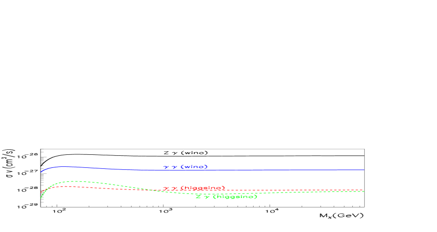
Figure 3: Dependence of the $\gamma\gamma$ and $Z\gamma$ cross sections as a function of the LSP neutralino mass $M_{\tilde{\chi}^{0}_{1}}$. For the higgsino case we take $M_{2}=2M_{1}=4\;10^{5}$TeV and for the wino $\mu=M_{1}=2\;10^{5}$TeV. In both cases $\tan\beta=10$, $M_{A}=100$TeV and all sfermions $4\;10^{5}$TeV. We use $M_{W}=M_{Z}c_{W}$, with $s_{W}=0.473$, $M_{Z}=91.1884$GeV, $\alpha^{-1}=127.9$.

The results of Table 1 make it clear that most interesting scenarios for the monochromatic $\gamma$ ray line signals are of a wino and higgsino type even when the LSP has a mass of about $2M_{Z}$. Fig. 3 shows the dependence of the $\tilde{\chi}^{0}_{1}\tilde{\chi}^{0}_{1}\rightarrow\gamma\gamma\;$and $\tilde{\chi}^{0}_{1}\tilde{\chi}^{0}_{1}\rightarrow Z\gamma\;$cross sections at $v=0$ as a function of the LSP mass in the case of a wino and a higgsino LSP. The mass of the LSP is in the range $70$GeV to $100$TeV. In fact masses below $100$GeV may be excluded by LEP2 but it is interesting to see how the cross sections grow past the $100$GeV mass to stabilise around a plateau. The masses of the other supersymmetric particles are taken extremely heavy here. Note that in the higgsino case $\tilde{\chi}^{0}_{1}\tilde{\chi}^{0}_{1}\rightarrow Z\gamma\;$shows much more structure. The peak cross section is much more pronounced before the cross section decreases and reaches a plateau of the same order as $\tilde{\chi}^{0}_{1}\tilde{\chi}^{0}_{1}\rightarrow\gamma\gamma\;$. The wino cross section for $\tilde{\chi}^{0}_{1}\tilde{\chi}^{0}_{1}\rightarrow Z\gamma\;$is the largest of all and is almost an order of magnitude larger than $\tilde{\chi}^{0}_{1}\tilde{\chi}^{0}_{1}\rightarrow\gamma\gamma\;$and two orders of magnitude larger than in the higgsino case.

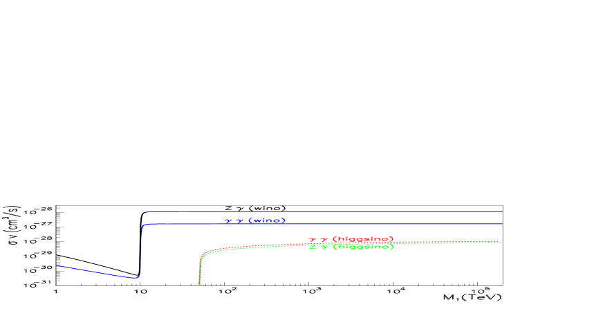
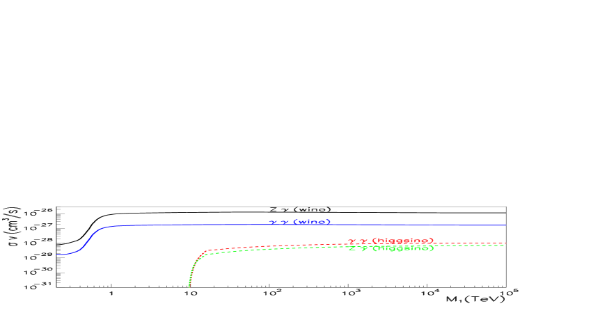
Figure 4: The first figure shows the dependence on $M_{1}$ for $\mu(M_{2})$ fixed in the higgsino (wino) limit for $\gamma\gamma$ and $Z\gamma$. The values for the SUSY parameters are: $\tan\beta=10$, $m_{\tilde{f}}=4\;10^{8}$GeV, $A=0$, $M_{A}=100$TeV. $\mu=50$TeV, $M_{2}=2M_{1}$ in the higgsino case. $M_{2}=10$TeV and $\mu=M_{1}$ in the wino case. In the figure at the bottom, the only parameters that are changed are $\mu=10$TeV in the higgsino case and $\tan\beta=2$, $M_{2}=500$GeV in the wino case. The SM parameters are as in Fig. 3.

It is also interesting to see how the plateau is reached for a fixed mass of the wino and higgsino LSP, or rather a fixed value of $M_{2}$ and $\mu$, depending on the composition of the LSP. We therefore fix these two values and vary the other supersymmetric parameters of the neutralino sector. The behaviour of the cross section as we vary these parameters is shown in Fig. 4. For the wino case one can see that once $M_{1},\mu>M_{2}$, and therefore the LSP is mostly wino, the asymptotic values are reached abruptly especially for the case of a wino of $10$TeV and large $\tan\beta$. Below this transition, the cross sections have a smooth behaviour. In the higgsino limit, a fast transition occurs once $M_{1},M_{2}>\mu$ but past this threshold there is still a smooth and slow increase of the cross sections before the asymptotic values are reached.

Most of this behaviour can, in fact, be recovered through simple analytical expressions that serve also as a further check on our results and the accuracy of the calculation in these extreme scenarios. It had been observed[9, 11] that when the LSP is heavy, much heavier that the $W$-boson, the cross sections (times velocity) for $\tilde{\chi}^{0}_{1}\tilde{\chi}^{0}_{1}\rightarrow\gamma\gamma\;$and $\tilde{\chi}^{0}_{1}\tilde{\chi}^{0}_{1}\rightarrow Z\gamma\;$tend to an asymptotic value that can be computed from the dominant contribution, that of diagram a) of Fig. 1. The limiting behaviour can be easily understood from the fact that in the heavy mass limit, the annihilating LSP neutralino and the chargino are degenerate with a mass much larger than the weak boson mass. This develops a threshold singularity like what one finds in QED, although here $M_{W}$ acts as a regulator. Another important factor that measures how the asymptotic values are reached is the deviation from exact degeneracy between the LSP neutralino and the lightest chargino given by their mass difference, $\delta m$, $\delta m=m_{\tilde{\chi}_{1}^{+}}-m_{\tilde{\chi}_{1}^{0}}$[14]. This scenario has been revisited in a series of excellent papers[14] where it has been shown how the one-loop calculation in these cases need to be improved through a non-relativistic treatment. Our aim here, in the rest of this section, is to see how our one-loop results can be made to match with the non-perturbative treatment. This paves the way to an implementation in a code for indirect detection that can be used in all generality like what we have started to do in micrOMEGAs.
First, we will show how our one-loop results effectively capture the behaviour of the cross sections in these scenarios and how the asymptotic value in the case of a wino is reached dramatically fast.
In the higgsino limit, $\mu\ll M_{1},M_{2}$. We will also take $M_{2}=2M_{1}=2M_{S}$ and consider also the large $\tan\beta$ (in fact $\tan\beta>2$ suffices). $\mu$ will be taken positive.
In the wino limit, $M_{2}\ll\mu,M_{1}$. We will also take $\mu=M_{1}=M_{S}$ and large $\tan\beta$. The (tree-level) mass difference in the higgsino, $\delta m^{\tilde{h}}$, and wino limit, $\delta m^{\tilde{w}}$, write

$$\delta m^{\tilde{h}} \simeq \frac{m_{Z}^{2}}{2M_{2}}c_{W}^{2}(1-\sin 2\beta)+\frac{m_{Z}^{2}}{2M_{1}}s_{W}^{2}(1+\sin 2\beta)\sim\frac{5}{16}\frac{M_{Z}^{2}}{M_{S}},$$

$$\delta m^{\tilde{w}} \simeq \frac{m_{Z}^{4}}{M_{1}\mu^{2}}s_{W}^{2}c_{W}^{2}\sin^{2}2\beta\sim\frac{M_{Z}^{2}M_{W}^{2}}{M_{S}^{3}}\frac{1}{\tan\beta^{2}}.$$ (1)

We see that in the wino case the mass difference scales like $1/M_{S}^{3}$[14] compared to the $1/M_{S}$ in the higgsino case. In these configurations the cross sections are well approximated[14] by $\tilde{\sigma}^{V\gamma,\tilde{h}}\;v$ in the higgsino case and $\tilde{\sigma}^{V\gamma,\tilde{w}}\;v$ in the wino case ($V=Z,\gamma$) which are the results of the dominant diagrams of Fig. 1-a),

$$\tilde{\sigma}^{V\gamma,\tilde{h}}\;v = \sigma_{\infty}^{V\gamma,\tilde{h}}v\left(1+\sqrt{\frac{2m_{\tilde{\chi}_{1}^{0}}\delta m}{M_{W}^{2}}}\right)^{-2}=\sigma_{\infty}^{V\gamma,\tilde{h}}v\left(1+\sqrt{\frac{5\mu}{6M_{S}}}\right)^{-2},$$

$$\tilde{\sigma}^{V\gamma,\tilde{w}}\;v = \sigma_{\infty}^{V\gamma,\tilde{w}}v\left(1+\sqrt{\frac{2M_{Z}^{2}M_{2}}{M_{S}^{3}\tan\beta^{2}}}\right)^{-2};\quad V=Z,\gamma.$$ (2)

where the asymptotic values ($\delta m=0$) are given by

$$\sigma_{\infty}^{\gamma\gamma,\tilde{h}}\;v = \frac{\alpha^{4}\pi}{4M_{W}^{2}s_{W}^{4}}\sim 10^{-28}cm^{3}/s,$$

$$\sigma_{\infty}^{\gamma\gamma,\tilde{w}}\;v = 16\sigma_{\infty}^{\gamma\gamma,\tilde{h}}\;v\sim 1.6\;10^{-27}cm^{3}/s,$$ (3)

$$\sigma_{\infty}^{Z\gamma,\tilde{h}}\;v = 2\frac{(1/2-s_{W}^{2})^{2}}{s_{W}^{2}c_{W}^{2}}\;\sigma_{\infty}^{\gamma\gamma,\tilde{h}}\;v\sim 0.8\;10^{-28}cm^{3}/s,$$ (4)

$$\sigma_{\infty}^{Z\gamma,\tilde{w}}\;v = 2\frac{c_{W}^{2}}{s_{W}^{2}}\;\sigma_{\infty}^{\gamma\gamma,\tilde{w}}\;v\sim 10^{-26}cm^{3}/s.$$ (5)

We have verified that our code including the complete contributions agrees extremely well with these approximation for the cross sections, Eq. 4, and that moreover in the wino case the asymptotic values, Eq. 4, are reached very fast due to very small $\delta m$. This is also exemplified in Fig. 4.

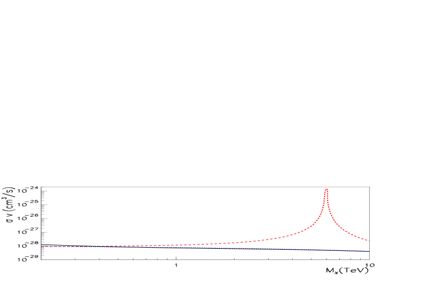
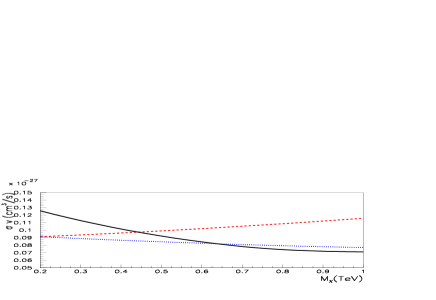
Figure 5: Comparison, for $\tilde{\chi}^{0}_{1}\tilde{\chi}^{0}_{1}\rightarrow\gamma\gamma\;$as a function $M_{\tilde{\chi}^{0}_{1}}$, between our prediction for the full one-loop calculation (continuous line, black), analytical one-loop expressions based on the approximation of Eq. 4 (dotted, blue) and the non-perturbative prediction based on the fitting functions including resonances[14] (dashed,red). The input susy parameters are $M_{2}=2M_{1}=50$TeV, $\tan\beta=10$, $A=0$, $m_{\tilde{f}}=M_{A}=100$TeV. The SM parameters are as in Fig. 3. The insert is a close-up for small $M_{\tilde{\chi}^{0}_{1}}$.

As demonstrated in [14] the one-loop treatment of the threshold singularity that is responsible for the behaviour of these cross sections in the higgsino and wino regime at high LSP mass is not adequate an breaks unitarity. The non-perturbative non-relativistic approach of Ref. [14] not only improves on the calculation but it also unravels the formation of bound states that drastically enhance the annihilation cross sections for specific combinations of masses. Fig. 5 shows the effect of such resonances and the departure of the cross section $\tilde{\chi}^{0}_{1}\tilde{\chi}^{0}_{1}\rightarrow\gamma\gamma\;$from a full one-loop treatment as the mass of the higgsino LSP increases. The “resonance” curve is based on the use of a fitting function as given in[14] . All other particles are taken heavy apart from the higgsino mass parameter $\mu$ and $M_{1}=M_{S}=M_{2}/2=25$TeV. For the whole range of $M_{\tilde{\chi}^{0}_{1}}\sim\mu$ we have $\delta m=0.1$GeV. The figure also shows the value of the approximate one-loop result as given for the higgsino limit in Eq. 4, together with the full one-loop treatment based on our calculation. The resonance formation, here around $6$TeV, brings an enhancement factor of more than $4$ orders of magnitude. On the other hand departure from the full one-loop calculation is of relevance only for $M_{\tilde{\chi}^{0}_{1}}$ masses around $1$TeV. The insert in Fig. 5 shows in more detail the comparison of the full calculation compared to the approximate result for the smaller higgsino LSP masses, well before the resonance effects settle in. For $M_{\tilde{\chi}^{0}_{1}}>600$GeV the approximation is very good, only around $M_{\tilde{\chi}^{0}_{1}}\sim 200$GeV, the full calculation captures the effect of other contributions like those of Fig. 1b,e). For this particular case it looks like a good matching between the full one-loop result and the non perturbative one should be made at around $M_{\tilde{\chi}^{0}_{1}}=400$GeV. A possible strategy for choosing this matching point would have to rely on the knowledge of both the full one-loop result, the approximate one-loop result as given Eq. 4 and the non-perturbative results based on the fitting functions of Ref. [14]. This would, of course, only be carried out in the limit of almost pure higgsino or wino. We would then have to compare the three results. To revert to the non-perturbative regime means that the full one-loop and the approximate one-loop agree fairly well and are quite different from the non-perturbative regime. If, on the other hand, these two one-loop results differ sensibly this means that one is not quite in the asymptotic region and that we might be missing some one-loop contributions. If this is the case one should also expect the higher order effects computed for the threshold region to be small so that the non-perturbative result and the approximate one-loop are very similar. Of course, as shown in the example of Fig. 5 these differences in the higgsino region, compared to taking the perturbative parameterisation, are rather small compared to the uncertainty that is inherent in the astrophysics part of the prediction of the gamma ray line. For the wino, as we saw, the transition to the asymptotic value is rather drastic especially for TeV LSP’s, therefore one should quickly capture the non-perturbative regime. Especially in this case one should also revert to a one-loop use of the chargino-LSP mass difference.

5 Conclusions

There has been a flurry of activity in the last few years in the search of dark matter with, among other strategies, many experiments dedicated to the indirect searches of dark matter in particular the gamma ray signal. The mono-energetic gamma ray line signal constitutes a clean signature. The improvement in coverage and accuracy of the measurements should be matched by precise theoretical calculations that should be publicly available through general purpose codes. In this paper we have provided a new calculation for $\tilde{\chi}^{0}_{1}\tilde{\chi}^{0}_{1}\rightarrow\gamma\gamma\;$and $\tilde{\chi}^{0}_{1}\tilde{\chi}^{0}_{1}\rightarrow Z\gamma\;$for the annihilation of the supersymmetric dark matter candidate and rederived as a bonus the $\tilde{\chi}^{0}_{1}\tilde{\chi}^{0}_{1}\rightarrow gg\;$rate. These calculations have been made both for small (zero) relative velocity of the neutralinos as adequate for annihilation in the halo of our galaxy for example, but also for velocities that would be needed for the contribution of these channels in a precise derivation of the relic density. For $\tilde{\chi}^{0}_{1}\tilde{\chi}^{0}_{1}\rightarrow\gamma\gamma\;$and $\tilde{\chi}^{0}_{1}\tilde{\chi}^{0}_{1}\rightarrow Z\gamma\;$at $v\neq 0$ as would be needed for an improved relic density prediction, these results are new. For $\tilde{\chi}^{0}_{1}\tilde{\chi}^{0}_{1}\rightarrow\gamma\gamma\;$three[9, 10] full one-loop calculations performed for $v=0$ have already been performed. We have performed a tuned comparison with the results of DarkSUSY[12] and PLATON[10] and have found perfect agreement. The calculation of $\tilde{\chi}^{0}_{1}\tilde{\chi}^{0}_{1}\rightarrow Z\gamma\;$is trickier and can not just be deduced from $\tilde{\chi}^{0}_{1}\tilde{\chi}^{0}_{1}\rightarrow\gamma\gamma\;$. Until now there has been only one calculation[11] of this process. The latter has missed some contributions that may not always be negligible. Comparisons of our results with the previous ones without these contributions are quite good for scenarios where the cross section is not small. In this paper we have not made an attempt to fold in with the astrophysics part that involves, for example, the halo profile but concentrated on the particle physics part which must be an unambiguous prediction. To pave the way for an implementation in micrOMEGAs[15] we felt it was important to critically review the large mass higgsino and wino LSP scenarios especially that the latter give large cross sections. As shown in[14] one needs to go beyond the one-loop treatment in this regime. We have argued how one could match the full one-loop treatment with the non-perturbative result.

Another important aspect of this paper is the way all these calculations have been performed in a unified manner and the techniques that we used. These processes are the first application of a code for the calculation of one-loop processes in supersymmetry both at the colliders and for astrophysics/relic density calculations that require also a new way of dealing with the reduction of the tensor integrals. The calculations are performed with the help of an automatised code that allows gauge parameter dependence checks to be performed. The use of a generalised non-linear gauge is crucial.

Acknowledgment
We acknowledge discussions with our other colleagues of the micrOMEGAs Project in particular G. Bélanger who made some early comparisons with DarkSUSY and A. Pukhov who made some test runs with the $\gamma\gamma$ and $Z\gamma$ annihilations routines within micrOMEGAs. P. Brun and S. Rosier-Lees also made some test runs for the gamma ray predictions using a private version of micrOMEGAs  for indirect detection and we gratefully thank them here. F.B. would like to thank the members of the Minami-Tateya group for important discussions and a fruitful collaboration. He also acknowledges discussions on the Gram determinant issue with T. Binoth, S. Dittmaier, J.P. Guillet and E. Pilon. F. Renard has been, as always, of invaluable help. We also thank J. Hisano and M. Nojiri for confirming that Eq. 61 of hep-ph/0412403 should be squared and that the entry $i=0,j=1$ in Table 1 of that paper is 10 times smaller. P. Gondolo has promptly provided us with the results of DarkSUSY reported in Table 1 and explained how to enter the parameters within this code for our tuned comparison. Fig. 1 and Fig. 2 are, in part, generated with JaxoDraw[37]. This work is supported in part by GDRI-ACPP of the CNRS (France). The work of A.S is supported by grants of the Russian Federal Agency of Science NS-1685.2003.2 and RFBR 04-02-17448 and that of D.T is supported, in part, by a postdoctoral grant from the Spanish Ministerio de Educacion y Ciencia.

A Appendix: Segmentation of loop integrals

The tensor integral of rank $M$ corresponding to a $N$-point graph, $\{M,N\}$, that we encounter in the general non-linear gauge but with Feynman parameters $\xi=1$ are such that $M\leq N$. For the evaluation of $2\rightarrow 2$ processes $N=4$ is the maximum value and corresponds to the box. The general tensor integral writes as

$$T_{\underbrace{\mu\nu\cdots\rho}_{M}}^{(N)}=\int\frac{d^{n}l}{(2\pi)^{n}}\;\frac{l_{\mu}l_{\nu}\cdots l_{\rho}}{D_{0}D_{1}\cdots D_{N-1}},\quad M\leq N,$$ (A. 1)

where

$$D_{i}=(l+s_{i})^{2}-M_{i}^{2},\quad s_{i}=\sum_{j=1}^{i}p_{j},\quad s_{0}=0.$$ (A. 2)

$M_{i}$ are the internal masses, $p_{i}$ the incoming momenta and $l$ the loop momentum.

The $N$-point scalar integrals correspond to $M=0$. All higher rank tensors for a $N$-point function, $M\geq 1$, can be deduced recursively from the knowledge of the $N$-point (and lower) scalar integrals. In Looptools[24] this is based on the Passarino-Veltman algorithm[31]. In Grace-loop the implementation is outlined in Ref. [21]. The tensor reduction involves solving, recursively, a system of equations which explicitly requires the evaluation of the Gram determinant: $DetG(p_{1},p_{2},p_{3})=DetG_{123}=Detp_{i}p_{j}$. For special kinematics the latter vanishes or can get very small, leading to severe numerical instability. This special kinematics for the general $2\rightarrow 2$ process one encounters in high energy occurs for exceptional points in phase space, for instance in extremely forward regions and most generally the weight of this contribution may be dismissed. For the case at hand, when the two neutralinos are at rest, or with extremely low relative velocity, the Gram determinant vanishes for all points because the incoming neutralinos have the same momentum and can not be considered independent. This is exactly what occurs in our case. Indeed here, the box diagrams for $\tilde{\chi}^{0}_{1}\tilde{\chi}^{0}_{1}\rightarrow Z\gamma\;$have the Gram determinant

$$DetG=M_{\tilde{\chi}^{0}_{1}}^{6}v^{2}\frac{\sin^{2}\theta}{(1-v^{2}/4)^{3}}(1-z^{2}),\quad z^{2}=\frac{M_{Z}^{2}}{4M_{\tilde{\chi}^{0}_{1}}^{2}}(1-v^{2}/4),$$ (A. 3)

$v$ is the relative velocity and $\theta$ is the scattering angle. For $\tilde{\chi}^{0}_{1}\tilde{\chi}^{0}_{1}\rightarrow\gamma\gamma\;$, $z=0$. In our application the sub-determinant with the incoming LSP neutralinos is responsible for the vanishing of the box Gram determinant for all angles:

$$DetG(p_{1},p_{2})=-M_{\tilde{\chi}^{0}_{1}}^{4}v^{2}\frac{1}{(1-v^{2}/4)^{2}}.$$ (A. 4)

This also means that the reduction of the tensor integrals for triangles with the two LSP as external legs, needs special treatment. Such triangles are of the type Fig. 1.e) (but not Fig.1 d)).

We therefore need to implement a routine for cases when the determinant vanishes due to the fact that the momenta $s_{i},i\neq 0$ are not independent. There are a few ways of dealing with the tensor integrals when the Gram determinant is exactly zero[32, 33]. Sometimes, the problem is even avoided by the grouping of terms so that this spurious inverse determinant cancels out. Our aim was to find, at least for $2\rightarrow 2$ process, an efficient method that can, not only be easily automated, but also calls most of the existing routines that are present for a general purpose algorithm designed for non zero Gram determinants. Take the box for example. Observe that (in any $n$ dimension), in most generality, we may write for any given pair of constants $\alpha,\beta$

$$\frac{1}{D_{0}D_{1}D_{2}D_{3}} = \left(\frac{1}{D_{0}D_{1}D_{2}}-\alpha\frac{1}{D_{0}D_{2}D_{3}}-\beta\frac{1}{D_{0}D_{1}D_{3}}+(\alpha+\beta-1)\frac{1}{D_{1}D_{2}D_{3}}\right)\times$$

$$\frac{1}{A+2l.(s_{3}-\alpha s_{1}-\beta s_{2})}$$

$$A = (s_{3}^{2}-M_{3}^{2})-\alpha(s_{1}^{2}-M_{1}^{2})-\beta(s_{2}^{2}-M_{2}^{2})-(\alpha+\beta-1)M_{0}^{2}.$$ (A. 5)

Obviously if $s_{3}=\alpha s_{1}+\beta s_{2}$ and hence the momenta are linearly dependent, the box splits into a sum of triangles. We will refer to this as segmentation. This segmentation is independent of the tensor structure. This means that the reduction of the tensor box with zero Gram determinant amounts to a tensor reduction for triangle with a non-zero Gram determinant for which one uses the usual procedure and hence uses the general library. Observe that if $\alpha=0$ or $\beta=0$, there are three segments instead of four. The missing segment, triangle integral, does in fact have a zero Gram determinant. Therefore when one approaches the zero of the Gram determinant of the box in these specific cases, $\alpha\sim 0$ for example, $\alpha$ will be numerically very small but non zero. A numerical instability could still develop due now to the Gram determinant of the associated triangle. These “algebraic” zeros could be missed at the numerical level. This can again lead to (less severe) numerical instabilities due to the reduction of the associated tensor. In this case, these triangles are segmented even further into two-point functions, following the same recipe. This way their contribution is negligible even at the numerical, automatic, level. In any case, since we also encounter (tensor) triangle diagrams (Fig. 1.e)) that have a vanishing Gram determinant, we have also included a segmentation that also applies to the tensor triangles using the same trick as for the boxes.

There is an important observation to make. The segmentation of a tensor of rank $M$ for the $N$-point function, $\{M,N\}$, amounts to applying the tensor reduction on $\{M,N-1\}$. If $M=N$, after segmentation one would need a library for $\{N,N-1\}$. These are not supplied by default in the general libraries. These libraries would then need to be extended. Reduction of $N-1$-point function tensor integrals are much more compact and easier than for $N$-point functions. This said for the case at hand, and for that matter any relic density calculation where the LSP is a neutralino, these highest rank tensors are not needed. It is easy to show that the highest rank tensors for $2\rightarrow 2$ only occurs when all the external particles are bosons. In our case, for the box, one has $M_{{\rm max}}=3$. For $\tilde{\chi}^{0}_{1}\tilde{\chi}^{0}_{1}\rightarrow f\bar{f}$, $M_{{\rm max}}=2$.

The choice of the momenta circulating in the loop, $s_{1},s_{2},s_{3}$, is not unique and depends on the particular graph. If $DetG(s_{1},s_{2},s_{3})=0$ we first form all three sub-determinants $DetG(s_{i},s_{j})$ and take the couple $s_{i},s_{j}$ that corresponds to $Max\;|Det(s_{i},s_{j})|$. Then the third $s_{k}$ is distributed in the basis $s_{i},s_{j}$ and the corresponding $\alpha$ and $\beta$ are read. In fact, suppose $DetG(s_{1},s_{2})\neq 0$, then it is revealing to always write

$$s_{3} = \alpha s_{1}+\beta s_{2}+\varepsilon_{T}\quad{\rm with}$$

$$s_{1}.\varepsilon_{T} = s_{2}.\varepsilon_{T}=0\quad{\rm meaning}$$

$$\varepsilon_{T,\mu} = \epsilon_{\mu\alpha\beta\delta}s_{1}^{\alpha}s_{2}^{\beta}t^{\delta}.$$ (A. 6)

$\varepsilon_{T}$ is a vector that is orthogonal to both $s_{1}$ and $s_{2}$ that is easily reconstructed once $\alpha$ and $\beta$ are

$$\alpha=\frac{s_{2}^{2}s_{3}.s_{1}-s_{1}.s_{2}s_{2}.s_{3}}{DetG(s_{1},s_{2})},\quad\beta=\alpha(s_{1}\leftrightarrow s_{2}).$$ (A. 7)

This construction makes it clear that

$$DetG(s_{1},s_{2},s_{3})=\varepsilon_{T}^{2}DetG(s_{1},s_{2}).$$ (A. 8)

This shows, in a most transparent manner, that the determinant vanishes when $\varepsilon_{T}^{2}=0$. This can occur when the components of this vector vanish, $\varepsilon_{T}^{\mu}\rightarrow 0$, and therefore $s_{3}$ is not an independent vector as the case of this paper for $v=0$. It also occurs, a point which is often overlooked, when $\varepsilon_{T}$ is light-like. However the orthogonality constraint means that the other vectors $s_{1},s_{2}$ are space-like. Therefore this case does not occur for real particles that are time-like, and hence does not occur for our $2\rightarrow 2$ process. It will be shown, in a separate publication, that when $\varepsilon_{T}$ is light-like a segmentation is still possible. The algorithm can also be improved by expanding around $DetG(s_{1},s_{2},s_{3})=0$. We will come back to the details of this issue in a future publication. Note that for $v=0.5$ and for all three processes studied in this paper the standard reduction formalism, without segmentation, was used.

References

-
[1]
The WMAP Collaboration, C. L. Bennett et al.,
Astrophys. J. Suppl. 148 (2003) 1; astro-ph/0302207.
D. N. Spergel et al., Astrophys. J. Suppl. 148 (2003) 175; astro-ph/0302209. -
[2]
K. Tsuchiya et al., The CANGAROO Collaboration,
Astrophys. J. Lett. 606; astro-ph/0403592.
H. Kubo et al., New Astronomy Reviews 48 (2004) 323.
http://icrhp9.icrr.u-tokyo.ac.jp/. - [3] J.A. Hinton, The HESS Collaboration, New Astron.Rev. 48 (2004) 331. http://www.mpi-hd.mpg.de/hfm/HESS/.
-
[4]
C. Baixeras, Nucl.Phys.B (Proc.Suppl.) 114 (2003) 247.
http://wwwmagic.mppmu.mpg.de/collaboration/. -
[5]
T.C. Weekes et al., Astropart. Phys. 17 (2002) 221.
http://veritas.sao.arizona.edu/. -
[6]
The AMS Collaboration, S. P. Ahlen et al., Nucl. Instrum. Meth. A 350, 351 (1994);
J. Alcaraz et al., Nucl. Instrum. Meth. A 478, 119 (2002);
http://ams.cern.ch/,. -
[7]
The EGRET Collaboration, R.C. Hartman et al.,
Astrophys.J.Suppl. (1999)
123:79.
http://egret0.stanford.edu/. -
[8]
See for instance, J. E. McEnery, I. V. Moskalenko and J. F. Ormes,
astro-ph/0406250.
The GLAST Collaboration, http://www-glast.sonoma.edu/. -
[9]
L. Bergström and P. Ullio, Nucl. Phys. 504 (1997) 27; hep-ph/9706232.
Z. Bern, P. Gondolo and M. Perelstein, Phys. Lett. B411 (1997) 86; hep-ph/9706538. -
[10]
G.J. Gounaris, J. Layssac, P.I. Porfyriadis and F.M. Renard,
Phys.Rev. D69 (2004) 075007; hep-ph/0309032. The PLATON codes may be downloaded
from
http://dtp.physics.auth.gr/platon/download.html. - [11] P. Ullio and L. Bergstrom, Phys.Rev.D57 (1998) 1962; hep-ph/9707333.
-
[12]
DarkSUSY: P. Gondolo et al., JCAP 0407:008,2004; astro-ph/0406204.
http://www.physto.se/edsjo/darksusy/. - [13] M. Drees, G. Jungman, M. Kamionkowski and M. M. Nojiri, Phys. Rev. D 49 (1994) 636; hep-ph/9306325.
-
[14]
J. Hisano, S. Matsumoto, M.M. Nojiri, Phys. Rev. D67
(2003) 075014; hep-ph/0212022.
ibid Phys.Rev.Lett. 92 (2004) 031303; hep-ph/0307216.
J. Hisano, S. Matsumoto, M.M. Nojiri and O. Saito, Phys.Rev. D71 (2005) 063528; hep-ph/0412403. -
[15]
G. Bélanger, F. Boudjema, A. Pukhov and A. Semenov, Comput.
Phys. Commun.
149 (2002) 103; hep-ph/0112278. ibid, Comput. Phys. Commun. in
Press, hep-ph/0405253.
http://wwwlapp.in2p3.fr/lapth/micromegas/. -
[16]
P. Brun, talk given at the French GdR SUSY, Grenoble, April 2005
http://lpsc.in2p3.fr/cdsagenda//askArchive.php?base=.agenda\&categ=a0540\&id=a0540s8t5/transparencies. -
[17]
G. Bélanger, F. Boudjema, J. Fujimoto, T. Ishikawa, T. Kaneko,
K. Kato and
Y. Shimizu, Phys. Lett. B559 (2003) 252; hep-ph/0212261.
G. Bélanger, F. Boudjema, J. Fujimoto, T. Ishikawa, T. Kaneko, K. Kato and Y. Shimizu, Phys. Lett. B559 (2003) 252; hep-ph/0212261.
G. Bélanger, F. Boudjema, J. Fujimoto, T. Ishikawa, T. Kaneko, K. Kato, Y. Shimizu and Y. Yasui, Phys.Lett. B571 (2003) 163; hep-ph/0307029.
G. Bélanger, F. Boudjema, J. Fujimoto, T. Ishikawa, T. Kaneko, Y. Kurihara, K. Kato, and Y. Shimizu, Phys. Lett. B576 (2003) 152; hep-ph/0309010.
F. Boudjema, J. Fujimoto, T. Ishikawa, T. Kaneko, K. Kato, Y. Kurihara, Y. Shimizu and Y. Yasui, Phys.Lett. B600 (2004) 65, hep-ph/0407065.
F. Boudjema, J. Fujimoto, T. Ishikawa, T. Kaneko, K. Kato, Y. Kurihara, Y. Shimizu, S. Yamashita and Y. Yasui, Nucl.Instrum.Meth. A534 (2004) 334; hep-ph/0404098. -
[18]
A. Denner, S. Dittmaier, M. Roth and M.M. Weber, Phys.Lett. B575
(2003) 290;
hep-ph/0307193. ibid Phys.Lett. B560 (2003) 196;
hep-ph/0301189.
Y. You, W. G. Ma, H. Chen, R. Y. Zhang, S. Yan-Bin and H. S. Hou, Phys. Lett. B 571 (2003) 85; hep-ph/0306036.
R. Y. Zhang, W. G. Ma, H. Chen, Y. B. Sun and H. S. Hou, Phys. Lett. B 578 (2004) 349; hep-ph/0308203. -
[19]
F. Boudjema, J. Fujimoto, T. Ishikawa, T. Kaneko, K. Kato,
Y. Kurihara and
Y. Shimizu,. KEK-CP-154, Nucl.Phys.Proc.Suppl.135 (2004) 323;
hep-ph/0407079.
F. Boudjema, J. Fujimoto, T. Ishikawa, T. Kaneko, K. Kato, Y. Kurihara, Y. Shimizu and Y. Yasui, presented by Y. Yasui at the ECFA Linear Collider Workshop, Durham, September 2004.http://conference.ippp.dur.ac.uk/cdsagenda//askArchive.php?base/.=agenda&categ=a041&id=a041s26t1/moreinfo/. - [20] A. Denner, S. Dittmaier, M. Roth and L.H. Wieders, Phys.Lett. B612 (2005) 223; hep-ph/0502063. ibid hep-ph/0505042.
- [21] G. Bélanger, F. Boudjema, J. Fujimoto, T. Ishikawa, T. Kaneko, K. Kato and Y. Shimizu, hep-ph/0308080.
-
[22]
T. Hahn and M. Perez-Victoria,Comp. Phys. Commun. 118 (1999)
153,
hep-ph/9807565.
T. Hahn, hep-ph/0406288, hep-ph/0506201. -
[23]
J. Küblbeck, M. Böhm, and A. Denner, Comp. Phys. Commun.
60 (1990)
165;
H. Eck and J. Küblbeck, Guide to FeynArts 1.0 (Würzburg, 1992);
H. Eck, Guide to FeynArts 2.0 (Würzburg, 1995);
T. Hahn, Comp. Phys. Commun. 140 (2001) 418, hep-ph/0012260. -
[24]
T. Hahn, LoopTools,
http://www.feynarts.de/looptools/. - [25] T. Hahn and C. Schappacher, Comp. Phys. Commun. 143 (2002) 54, hep-ph/0105349.
- [26] J. Fujimoto et al., Comput. Phys. Commun. 153 (2003) 106;hep-ph/0208036.
- [27] J. Fujimoto, T. Ishikawa, M. Jimbo, T. Kon and M. Kuroda, Nucl. Instrum. Meth. A 534 (2004) 246; hep-ph/0402145.
-
[28]
A. Semenov LanHEP — a package for automatic generation of
Feynman
rules. User’s manual. INP MSU 96–24/431, Moscow, 1996; hep-ph/9608488
A. Semenov. Nucl.Inst.&Meth. A393 (1997) p. 293.
A. Semenov. Comp. Phys. Comm., Vol. 115 (1998) 124.
A. Semenov, LAPTH-926/02; hep-ph/0208011. - [29] A. Pukhov et al., ”CompHEP user’s manual, v3.3”, Preprint INP MSU 98-41/542, 1998; hep-ph/9908288.
- [30] F. Boudjema and E. Chopin, Z.Phys. C73 (1996) 85; hep-ph/9507396.
- [31] G. Passarino and M. Veltman, Nucl. Phys. 160 (1979) 151.
- [32] T. Binoth, J. P. Guillet, G. Heinrich, E. Pilon and C. Schubert, hep-ph/0504267.
-
[33]
R. G. Stuart, Comput.Phys.Commun. 48 (1988) 367.
R. G. Stuart and A. Gongora, Comput. Phys. Commun. 56 (1990) 337.
R. G. Stuart, Comput. Phys. Commun. 85 (1995) 267; hep-ph/9409273.
G. Devaraj and R.G. Stuart, Nucl.Phys. B519 (1998) 483; hep-ph/9704308. - [34] H. E. Haber and D. Wyler, Nucl. Phys. B323 (1989) 267.
- [35] F. Boudjema and A. Semenov, Phys.Rev. D66 (2002) 095007; hep-ph/0201219.
- [36] B.C. Allanach, G. Bélanger, F. Boudjema and A. Pukhov, JHEP 0412 (2004) 020; hep-ph/0410091.
- [37] D. Binosi, L. Theussl, Comput.Phys.Commun. 161 (2004) 76; hep-ph/0309015.