June 2005 CERN–TH/2005–106
IPPP/05/25 DCTP/05/50
DFTT–17/05

Gluino Decays in Split Supersymmetry

P. Gambino${}^{\,a}$, G.F. Giudice${}^{\,b}$, P. Slavich${}^{\,c}$

^a INFN, Torino & Dip. Fisica Teorica, Univ. di Torino, I–10125 Torino, Italy
^b CERN, Theory Division, CH–1211 Geneva 23, Switzerland
^c Durham University, IPPP, DH1–3LE Durham, United Kingdom

We compute the gluino lifetime and branching ratios in Split Supersymmetry. Using an effective–theory approach, we resum the large logarithmic corrections controlled by the strong gauge coupling and the top Yukawa coupling. We find that the resummation of the radiative corrections has a sizeable numerical impact on the gluino decay width and branching ratios. Finally, we discuss the gluino decays into gravitino, relevant in models with direct mediation of supersymmetry breaking.

1 Introduction

The long gluino lifetime is a trademark of Split Supersymmetry [1, 2, 3]. The experimental discovery of a slowly–decaying gluino [4] would not only be a strong indication for Split Supersymmetry, but it would also allow for a measurement of the effective supersymmetry–breaking scale $\widetilde{m}$, which cannot be directly extracted from particle dynamics at the LHC. Moreover, the gluino lifetime is a crucial parameter to determine the cosmological constraints on the theory [1, 5]. Therefore, for both experimental and theoretical considerations, it is very important to have a precise prediction of the gluino lifetime and branching ratios.

For what concerns the gluino decay processes in the MSSM, tree–level results for the decays into chargino or neutralino and two quarks and one–loop results for the radiative decay into neutralino and gluon can be found in the literature [6]. In Split Supersymmetry, however, the quantum corrections to the gluino decay processes can be very significant, because they are enhanced by the potentially large logarithm of the ratio between the gluino mass $m_{\tilde{g}}$ and the scale $\widetilde{m}$ at which the interactions responsible for gluino decay are mediated. A fixed–order calculation of these processes in Split Supersymmetry would miss terms that are enhanced by higher powers of the large logarithm. In order to get a reliable prediction for the gluino decay width, the large logarithmic corrections have to be resummed by means of standard renormalization group techniques.

Recently, a calculation of the gluino decay widths in Split Supersymmetry was presented in ref. [7], working at tree level for 3–body decays and in (not resummed) one–loop approximation for 2–body decays. In this paper we will present a calculation of the gluino decay processes that includes all leading corrections in $\alpha_{s}$ and $\alpha_{t}$, the strong and top–Yukawa coupling constants. As we will show, the inclusion and resummation of leading–order corrections give sizeable modifications of the gluino branching ratios, even for moderate values of $\widetilde{m}$.

The structure of the paper is as follows: in sect. 2 we list the operators in the effective Lagrangian of Split Supersymmetry that are responsible for the decays of the gluino, and the high–energy boundary conditions on the corresponding Wilson coefficients; in sect. 3 we determine the renormalization group evolution of the Wilson coefficients, and we express the operators in the low–energy effective Lagrangian in terms of mass eigenstates; in sect. 4 we discuss our numerical results for the branching ratios and total width of the gluino decays in Split Supersymmetry; in sect. 5 we consider the possibility of gluinos decaying into gravitino; in sect. 6 we present our conclusions. Finally, in the appendix we provide the analytical formulae for the gluino decay widths.

2 The Effective Lagrangian

Below the squark and slepton mass scale $\widetilde{m}$, the effective Lagrangian of Split Supersymmetry describes the dynamics of Standard Model (SM) particles together with higgsinos and gauginos. At the level of renormalizable interactions, there is a conserved $G$–parity (under which only the gluino is odd) preventing gluino decay. However, integrating the squarks out of the underlying supersymmetric theory induces non–renormalizable interactions that violate the $G$–parity. Restricting our analysis up to dimension–6 operators, the $G$–odd effective Lagrangian at the matching scale $\widetilde{m}$ is given by

$${\cal L}=\frac{1}{\widetilde{m}^{2}}\,\sum_{i=1}^{7}C^{\,\widetilde{\scriptscriptstyle B}}_{i}\,Q^{\,\widetilde{\scriptscriptstyle B}}_{i}\;+\;\frac{1}{\widetilde{m}^{2}}\,\sum_{i=1}^{2}C^{\,\widetilde{\scriptscriptstyle W}}_{i}\,Q^{\,\widetilde{\scriptscriptstyle W}}_{i}\;+\;\frac{1}{\widetilde{m}^{2}}\,\left(\sum_{i=1}^{5}C^{\,\widetilde{\scriptscriptstyle H}}_{i}\,Q^{\,\widetilde{\scriptscriptstyle H}}_{i}+{\rm h.c.}\right).$$ (1)

We are working in the basis of interaction eigenstates for gauginos and higgsinos, neglecting the effect of electroweak symmetry breaking, since $\widetilde{m}\gg M_{Z}$. The $G$–odd operators involving the $B$–ino ($\widetilde{B}$) are

$$Q^{\,\widetilde{\scriptscriptstyle B}}_{1} = \overline{\widetilde{B}}\,\gamma^{\mu}\,\gamma_{5}\,{\tilde{g}}^{a}\;\otimes\;\sum_{k=1}^{2}\;\overline{q}_{\scriptscriptstyle L}^{\,(k)}\,\gamma_{\mu}\,T^{a}\,q_{\scriptscriptstyle L}^{\,(k)}$$ (2)

$$Q^{\,\widetilde{\scriptscriptstyle B}}_{2} = \overline{\widetilde{B}}\,\gamma^{\mu}\,\gamma_{5}\,{\tilde{g}}^{a}\;\otimes\;\sum_{k=1}^{2}\;\overline{u}_{\scriptscriptstyle R}^{\,(k)}\,\gamma_{\mu}\,T^{a}\,u_{\scriptscriptstyle R}^{\,(k)}$$ (3)

$$Q^{\,\widetilde{\scriptscriptstyle B}}_{3} = \overline{\widetilde{B}}\,\gamma^{\mu}\,\gamma_{5}\,{\tilde{g}}^{a}\;\otimes\;\sum_{k=1}^{2}\;\overline{d}_{\scriptscriptstyle R}^{\,(k)}\,\gamma_{\mu}\,T^{a}\,d_{\scriptscriptstyle R}^{\,(k)}$$ (4)

$$Q^{\,\widetilde{\scriptscriptstyle B}}_{4} = \overline{\widetilde{B}}\,\gamma^{\mu}\,\gamma_{5}\,{\tilde{g}}^{a}\;\otimes\;\overline{q}_{\scriptscriptstyle L}^{\,(3)}\,\gamma_{\mu}\,T^{a}\,q_{\scriptscriptstyle L}^{\,(3)}$$ (5)

$$Q^{\,\widetilde{\scriptscriptstyle B}}_{5} = \overline{\widetilde{B}}\,\gamma^{\mu}\,\gamma_{5}\,{\tilde{g}}^{a}\;\otimes\;\overline{t}_{\scriptscriptstyle R}\,\gamma_{\mu}\,T^{a}\,t_{\scriptscriptstyle R}$$ (6)

$$Q^{\,\widetilde{\scriptscriptstyle B}}_{6} = \overline{\widetilde{B}}\,\gamma^{\mu}\,\gamma_{5}\,{\tilde{g}}^{a}\;\otimes\;\overline{b}_{\scriptscriptstyle R}\,\gamma_{\mu}\ T^{a}\,b_{\scriptscriptstyle R}$$ (7)

$$Q^{\,\widetilde{\scriptscriptstyle B}}_{7} = \overline{\widetilde{B}}\,\sigma^{\mu\nu}\,\gamma_{5}\,{\tilde{g}}^{a}\;G^{a}_{\mu\nu},$$ (8)

where $k$ is a generation index, $T^{a}$ are the SU(3) generators and $G^{a}_{\mu\nu}$ is the gluon field strength. Assuming that the squark mass matrices are flavour–diagonal, the Wilson coefficients of the operators $Q^{\,\widetilde{\scriptscriptstyle B}}_{i}$ at the matching scale $\widetilde{m}$ are

$$C^{\,\widetilde{\scriptscriptstyle B}}_{1}(\widetilde{m})=C^{\,\widetilde{\scriptscriptstyle B}}_{4}(\widetilde{m})=-\frac{g_{s}\,g^{\prime}}{6}\,r_{\tilde{q}_{\scriptscriptstyle L}}\,, C^{\,\widetilde{\scriptscriptstyle B}}_{2}(\widetilde{m})=C^{\,\widetilde{\scriptscriptstyle B}}_{5}(\widetilde{m})=\frac{2\,g_{s}\,g^{\prime}}{3}\,r_{\tilde{u}_{\scriptscriptstyle R}}\,,$$ (9)

$$C^{\,\widetilde{\scriptscriptstyle B}}_{3}(\widetilde{m})=C^{\,\widetilde{\scriptscriptstyle B}}_{6}(\widetilde{m})=-\frac{g_{s}\,g^{\prime}}{3}\,r_{\tilde{d}_{\scriptscriptstyle R}}\,, C^{\,\widetilde{\scriptscriptstyle B}}_{7}(\widetilde{m})=\frac{g_{s}^{2}\,g^{\prime}}{128\,\pi^{2}}\,(m_{\tilde{g}}-m_{\scriptscriptstyle\widetilde{B}})\,\sum_{q}\,(r_{\tilde{q}_{\scriptscriptstyle L}}-r_{\tilde{q}_{\scriptscriptstyle R}})\,Q_{q}\,,$$ (10)

where $r_{\tilde{q}}=\widetilde{m}^{2}/m_{\tilde{q}}^{2}$. Note that $C^{\,\widetilde{\scriptscriptstyle B}}_{7}$ vanishes for mass–degenerate squarks.

The $G$–odd operators involving the $W$–ino ($\widetilde{W}$) are

$$Q^{\,\widetilde{\scriptscriptstyle W}}_{1} = \overline{\widetilde{W}^{\scriptscriptstyle A}}\,\gamma^{\mu}\,\gamma_{5}\,{\tilde{g}}^{a}\;\otimes\;\sum_{k=1}^{2}\;\overline{q}_{\scriptscriptstyle L}^{\,(k)}\,\gamma^{\mu}\,\tau^{\scriptscriptstyle A}\,T^{a}\,q_{\scriptscriptstyle L}^{\,(k)}$$ (11)

$$Q^{\,\widetilde{\scriptscriptstyle W}}_{2} = \overline{\widetilde{W}^{\scriptscriptstyle A}}\,\gamma^{\mu}\,\gamma_{5}\,{\tilde{g}}^{a}\;\otimes\;\overline{q}_{\scriptscriptstyle L}^{\,(3)}\,\gamma^{\mu}\,\tau^{\scriptscriptstyle A}\,T^{a}\,q_{\scriptscriptstyle L}^{\,(3)},$$ (12)

where $\tau^{\scriptscriptstyle A}$ are the Pauli matrices. The matching conditions for the Wilson coefficients are

$$C^{\,\widetilde{\scriptscriptstyle W}}_{1}(\widetilde{m})=C^{\,\widetilde{\scriptscriptstyle W}}_{2}(\widetilde{m})=-\frac{g_{s}\,g}{2}\,r_{\tilde{q}_{\scriptscriptstyle L}}.$$ (13)

For the higgsinos, we use a compact notation in which the two Weyl states $\widetilde{H}_{u}$ and $\widetilde{H}_{d}$ are combined in a single Dirac fermion $\widetilde{H}\equiv\widetilde{H}_{u}+\varepsilon\,\widetilde{H}_{d}^{c}$, where $\varepsilon$ is the antisymmetric matrix (with $\varepsilon_{12}=1$) acting on the SU(2) indices. The states $\widetilde{H}_{u}$ and $\widetilde{H}_{d}$ can be recovered by chiral decomposition, $\widetilde{H}_{u}=\widetilde{H}_{\scriptscriptstyle L}$ and $\widetilde{H}_{d}=-\varepsilon\,(\widetilde{H}^{c})_{\scriptscriptstyle L}$. Keeping only the third–generation Yukawa couplings, the $G$–odd operators involving higgsinos are

$$Q^{\,\widetilde{\scriptscriptstyle H}}_{1} = \overline{\widetilde{H}}_{\scriptscriptstyle L}\,{\tilde{g}}^{a}_{\scriptscriptstyle R}\;\otimes\;\varepsilon\,\overline{q}_{\scriptscriptstyle L}^{\,(3)}\,T^{a}\,t_{\scriptscriptstyle R}$$ (14)

$$Q^{\,\widetilde{\scriptscriptstyle H}}_{2} = \overline{\widetilde{H}}_{\scriptscriptstyle L}\,\sigma^{\mu\nu}\,{\tilde{g}}^{a}_{\scriptscriptstyle R}\;\otimes\;\varepsilon\,\overline{q}_{\scriptscriptstyle L}^{\,(3)}\,\sigma_{\mu\nu}\,T^{a}\,t_{\scriptscriptstyle R}$$ (15)

$$Q^{\,\widetilde{\scriptscriptstyle H}}_{3} = \overline{\widetilde{H}}_{\scriptscriptstyle R}\,{\tilde{g}}^{a}_{\scriptscriptstyle L}\;\otimes\;\overline{b}_{\scriptscriptstyle R}\,T^{a}\,q_{\scriptscriptstyle L}^{\,(3)}$$ (16)

$$Q^{\,\widetilde{\scriptscriptstyle H}}_{4} = \overline{\widetilde{H}}_{\scriptscriptstyle R}\,\sigma^{\mu\nu}\,{\tilde{g}}^{a}_{\scriptscriptstyle L}\;\otimes\;\overline{b}_{\scriptscriptstyle R}\,\sigma_{\mu\nu}\,T^{a}\,q_{\scriptscriptstyle L}^{\,(3)}$$ (17)

$$Q^{\,\widetilde{\scriptscriptstyle H}}_{5} = \overline{\widetilde{H}}_{\scriptscriptstyle L}\,\sigma^{\mu\nu}\,{\tilde{g}}^{a}_{\scriptscriptstyle R}\;h\;G^{a}_{\mu\nu},$$ (18)

where $h$ is the Higgs doublet. The Wilson coefficients at the matching scale $\widetilde{m}$ are

$$C^{\,\widetilde{\scriptscriptstyle H}}_{1}(\widetilde{m})=\frac{g_{s}\,h_{t}}{\sqrt{2}\sin\beta}\,(r_{\tilde{q}_{\scriptscriptstyle L}}-r_{\tilde{u}_{\scriptscriptstyle R}})\,,\;\;\;\;\;\;C^{\,\widetilde{\scriptscriptstyle H}}_{2}(\widetilde{m})=\frac{g_{s}\,h_{t}}{4\,\sqrt{2}\sin\beta}\,(r_{\tilde{q}_{\scriptscriptstyle L}}+r_{\tilde{u}_{\scriptscriptstyle R}})\,,$$ (19)

$$C^{\,\widetilde{\scriptscriptstyle H}}_{3}(\widetilde{m})=\frac{g_{s}\,h_{b}}{\sqrt{2}\cos\beta}\,(r_{\tilde{q}_{\scriptscriptstyle L}}-r_{\tilde{d}_{\scriptscriptstyle R}})\,,\;\;\;\;\;\;C^{\,\widetilde{\scriptscriptstyle H}}_{4}(\widetilde{m})=-\frac{g_{s}\,h_{b}}{4\,\sqrt{2}\cos\beta}\,(r_{\tilde{q}_{\scriptscriptstyle L}}+r_{\tilde{d}_{\scriptscriptstyle R}})\,,$$ (20)

$$C^{\,\widetilde{\scriptscriptstyle H}}_{5}(\widetilde{m})=\frac{g_{s}^{2}\,h_{t}^{2}}{32\,\sqrt{2}\,\pi^{2}\,\sin\beta}(r_{\tilde{q}_{\scriptscriptstyle L}}+r_{\tilde{u}_{\scriptscriptstyle R}}).$$ (21)

Here $h_{t}$ and $h_{b}$ are the top and bottom Yukawa couplings, and $\tan\beta$ is a free parameter of Split Supersymmetry.

Before proceeding to the operator renormalization, we want to make some remarks.

(i) We recall that all coupling constants appearing in the expressions of the Wilson coefficients given above have to be computed at the scale $\widetilde{m}$.

(ii) Note that we have given the Wilson coefficients of the 4–fermion operators at the leading perturbative order, while the coefficients of the operators $Q^{\,\widetilde{\scriptscriptstyle B}}_{7}$ and $Q^{\,\widetilde{\scriptscriptstyle H}}_{5}$ are given at the next order (one–loop approximation). The operator anomalous dimensions will be computed in sect. 3 at the leading order in the strong and top–Yukawa couplings $\alpha_{s}=g_{s}^{2}/(4\pi)$ and $\alpha_{t}=h_{t}^{2}/(4\pi)$. Therefore, the gluino 3–body decays, mediated only by 4–fermion operators, will be computed by resumming all $\alpha_{s,t}\ln(\widetilde{m}/m_{\tilde{g}})$ corrections, but neglecting terms ${\cal O}[\alpha^{n+1}_{s,t}\ln^{n}(\widetilde{m}/m_{\tilde{g}})]$ with $n\geq 0$. For the radiative 2–body gluino decay into a gluon and a neutralino, a greater accuracy is more appropriate. The expressions of $C^{\,\widetilde{\scriptscriptstyle B}}_{7}$ and $C^{\,\widetilde{\scriptscriptstyle H}}_{5}$ given in eqs. (10) and (21), together with leading–order anomalous dimensions and one–loop matrix elements [see eq. (62) below], allow us to determine the 2–body decay amplitude neglecting terms ${\cal O}[\alpha^{n+1}_{s,t}\ln^{n}(\widetilde{m}/m_{\tilde{g}})]$ with $n\geq 1$. This means that we have resummed all large logarithms at the leading order in all cases, but our formulae for 2–body gluino decays contain also the complete ${\cal O}(\alpha_{s,t})$ terms, relevant when the logarithm is not large.

(iii) If $\widetilde{m}$ is close to the GUT scale, in presence of gauge–coupling unification there is no solid justification for the approximation of computing $\alpha_{s}$ contributions to the anomalous dimensions, neglecting electroweak corrections. However, because of the large SU(3) coefficients, we consider our approximation to be fairly adequate, even for $\widetilde{m}$ as large as $10^{13}$ GeV, which is the maximum value of $\widetilde{m}$ consistent with the negative searches for anomalous heavy isotopes.

(iv) In eq. (20) we have included the contribution from the bottom Yukawa coupling $h_{b}$, since these coefficients are enhanced when $\tan\beta$ is large. There are no $\tan\beta$ enhancements in the evolution below $\widetilde{m}$, and therefore our results are reliable for any value of $\tan\beta$.

(v) Split Supersymmetry is free from flavour problems, therefore our assumption that squark mass matrices are diagonal is unnecessary. On the other hand, a certain degree of mass degeneracy among squarks is required by gauge-coupling unification. In the results presented in sect. 4 we take for simplicity all squark masses to be equal.

3 Operator Renormalization

The renormalization–group flow for the Wilson coefficients is determined by the equations

$$\mu\frac{d\vec{C}}{d\mu} = {\hat{\gamma}}^{T}(\alpha_{s},\alpha_{t})\,\vec{C}$$ (22)

$$\mu\frac{d\alpha_{s}}{d\mu} = -\beta_{s}\,\frac{\alpha_{s}^{2}}{2\pi}$$ (23)

$$\mu\frac{d\alpha_{t}}{d\mu} = -\beta_{t}\,\frac{\alpha_{t}^{2}}{2\pi}-\beta_{st}\frac{\alpha_{s}\alpha_{t}}{2\pi},$$ (24)

where $\mu$ is the renormalization scale and, in Split Supersymmetry, we have $\beta_{s}=5$, $\beta_{t}=-9/2$ and $\beta_{st}=8$. The anomalous–dimension matrix $\hat{\gamma}$ can be expressed as

$${\hat{\gamma}}_{ij}=-2\,b_{ij}-\delta_{ij}\sum_{f}a_{f},$$ (25)

where $b_{ij}$ are extracted from the poles of the one–loop renormalization of the operators $Q_{i}$ ($Q_{i}\rightarrow b_{ij}\,Q_{j}/\epsilon+\cdots$). In eq. (25) the sum is over all fields entering the operator $Q_{i}$, and the field anomalous dimensions $a_{f}$ are given by

$$a_{q^{k}_{\scriptscriptstyle L}}=-\frac{1}{4\,\pi}\left(\alpha_{s}\,C_{F}+\frac{\alpha_{t}}{2}\,\delta_{k3}\right)\,,\;\;\;\;\;a_{u^{k}_{\scriptscriptstyle R}}=-\frac{1}{4\,\pi}\left(\alpha_{s}\,C_{F}+\alpha_{t}\,\delta_{k3}\right)\,,\;\;\;\;\;a_{d_{\scriptscriptstyle R}}=-\frac{\alpha_{s}\,C_{F}}{4\,\pi}\,,$$ (26)

$$a_{\tilde{g}}=-\frac{\alpha_{s}\,N_{c}}{4\,\pi}\,,\;\;\;\;\;a_{h}=-\frac{\alpha_{t}\,N_{c}}{4\,\pi}\,,\;\;\;\;\;a_{g}=\frac{\alpha_{s}}{4\,\pi}\;\left(N_{c}-\frac{2}{3}\,N_{f}\right).$$ (27)

Here $k$ is a generation index, $C_{F}=(N_{c}^{2}-1)/(2N_{c})$, $N_{c}=3$, $N_{f}=6$. Note that the gluon anomalous dimension $a_{g}$ (given here in the Feynman gauge) is different from the SM value because it includes the gluino contribution.

We find that the anomalous–dimension matrices of the $B$–ino operators in eqs. (2)–(8), of the $W$–ino operators in eqs. (11)–(12), and of the higgsino operators in eqs. (14)–(18) are respectively

$${\hat{\gamma}}^{(a)}=\frac{\alpha_{s}}{4\pi}\gamma_{s}^{a}+\frac{\alpha_{t}}{4\pi}\gamma_{t}^{a}+\frac{\sqrt{\alpha_{s}\alpha_{t}}}{4\pi}\gamma_{st}^{a},~{}~{}~{}~{}a=\widetilde{\scriptscriptstyle B},\widetilde{\scriptscriptstyle W},\widetilde{\scriptscriptstyle H}$$ (28)

$$\gamma_{s}^{\widetilde{\scriptscriptstyle B}}=\frac{1}{3}\pmatrix{8-9N_{c}&8&8&8&8&8&0\cr 4&4-9N_{c}&4&4&4&4&0\cr 4&4&4-9N_{c}&4&4&4&0\cr 4&4&4&4-9N_{c}&4&4&0\cr 2&2&2&2&2-9N_{c}&2&0\cr 2&2&2&2&2&2-9N_{c}&0\cr 0&0&0&0&0&0&2N_{f}-18N_{c}},$$ (29)

$$\gamma_{t}^{\widetilde{\scriptscriptstyle B}}=\pmatrix{0&0&0&0&0&0&0\cr 0&0&0&0&0&0&0\cr 0&0&0&0&0&0&0\cr 0&0&0&1&\!\!\!\!-2&0&0\cr 0&0&0&\!\!\!\!-1&2&0&0\cr 0&0&0&0&0&0&0\cr 0&0&0&0&0&0&0},~{}~{}~{}~{}\gamma_{st}^{\widetilde{\scriptscriptstyle B}}=0,$$ (30)

$$\gamma_{s}^{\widetilde{\scriptscriptstyle W}}=\pmatrix{-3N_{c}&0\cr 0&-3N_{c}},~{}~{}~{}~{}\gamma_{t}^{\widetilde{\scriptscriptstyle W}}=\pmatrix{0&0\cr 0&1},~{}~{}~{}~{}\gamma_{st}^{\widetilde{\scriptscriptstyle W}}=0,$$ (31)

$$\gamma_{s}^{\widetilde{\scriptscriptstyle H}}=\pmatrix{\frac{3}{N_{c}}&0&0&0&0\cr 0&-4N_{c}-\frac{1}{N_{c}}&0&0&0\cr 0&0&\frac{3}{N_{c}}&0&0\cr 0&0&0&-4N_{c}-\frac{1}{N_{c}}&0\cr 0&0&0&0&\frac{2}{3}N_{f}-6N_{c}},$$ (32)

$$\gamma_{t}^{\widetilde{\scriptscriptstyle H}}=\frac{1}{2}\pmatrix{3&0&0&0&0\cr 0&3&0&0&0\cr 0&0&1&0&0\cr 0&0&0&1&0\cr 0&0&0&0&2N_{c}},~{}~{}~{}~{}\gamma_{st}^{\widetilde{\scriptscriptstyle H}}=\pmatrix{0&0&0&0&0\cr 0&0&0&0&4\cr 0&0&0&0&0\cr 0&0&0&0&0\cr 0&2&0&0&0}.$$ (33)

For coefficients with only multiplicative renormalization (which is the case for $C^{\,\widetilde{\scriptscriptstyle B}}_{7}$, $C^{\,\widetilde{\scriptscriptstyle W}}_{1,2}$, $C^{\,\widetilde{\scriptscriptstyle H}}_{1,3,4}$), eq. (22) can be easily integrated, with the result

$$C_{i}(\mu)=C_{i}(\widetilde{m})\,\eta_{s}^{\left(\frac{\gamma_{s}}{2\beta_{s}}-\frac{\beta_{st}\gamma_{t}}{2\beta_{s}\beta_{t}}\right)}\ \eta_{t}^{\frac{\gamma_{t}}{2\beta_{t}}}~{}~{}~{}~{}~{}{\rm for~{}~{}}C_{i}=C^{\,\widetilde{\scriptscriptstyle B}}_{7},~{}C^{\,\widetilde{\scriptscriptstyle W}}_{1,2},~{}C^{\,\widetilde{\scriptscriptstyle H}}_{1,3,4}.$$ (34)

We have defined

$$\eta_{s}\equiv\frac{\alpha_{s}(\widetilde{m})}{\alpha_{s}(\mu)} = 1+\frac{\alpha_{s}(\widetilde{m})}{2\pi}\beta_{s}\ln\frac{\mu}{\widetilde{m}}\,,$$ (35)

$$\eta_{t}\equiv\frac{\alpha_{t}(\widetilde{m})}{\alpha_{t}(\mu)} = \eta_{s}^{\frac{\beta_{st}}{\beta_{s}}}+\frac{\alpha_{t}(\widetilde{m})\beta_{t}}{\alpha_{s}(\widetilde{m})\left(\beta_{st}-\beta_{s}\right)}\left(\eta_{s}^{\frac{\beta_{st}}{\beta_{s}}}-\eta_{s}\right).$$ (36)

The evolution of the Wilson coefficients for the other $B$–ino operators involves operator mixing and the solution of eq. (22) is given by

$$C^{\,\widetilde{\scriptscriptstyle B}}_{i}(\mu) = \eta_{s}^{-\frac{9}{10}}\left[C^{\,\widetilde{\scriptscriptstyle B}}_{i}(\widetilde{m})+y\,{\overline{C}}(\widetilde{m})\right]~{}~{}~{}~{}i=1,2,3,6$$ (37)

$$C^{\,\widetilde{\scriptscriptstyle B}}_{4}(\mu) = \eta_{s}^{-\frac{9}{10}}\left[(1+z)\,C^{\,\widetilde{\scriptscriptstyle B}}_{4}(\widetilde{m})-z\,C^{\,\widetilde{\scriptscriptstyle B}}_{5}(\widetilde{m})+y\,{\overline{C}}(\widetilde{m})\right],$$ (38)

$$C^{\,\widetilde{\scriptscriptstyle B}}_{5}(\mu) = \eta_{s}^{-\frac{9}{10}}\left[(1+2z)\,C^{\,\widetilde{\scriptscriptstyle B}}_{5}(\widetilde{m})-2z\,C^{\,\widetilde{\scriptscriptstyle B}}_{4}(\widetilde{m})+y\,{\overline{C}}(\widetilde{m})\right],$$ (39)

where ${\overline{C}}=C^{\,\widetilde{\scriptscriptstyle B}}_{1}/3+(C^{\,\widetilde{\scriptscriptstyle B}}_{2}+C^{\,\widetilde{\scriptscriptstyle B}}_{3}+C^{\,\widetilde{\scriptscriptstyle B}}_{4})/6+(C^{\,\widetilde{\scriptscriptstyle B}}_{5}+C^{\,\widetilde{\scriptscriptstyle B}}_{6})/12$, $y=\eta_{s}^{\,4/5}-1$, and $z=(\eta_{s}^{\,8/15}\,\eta_{t}^{-1/3}-1)/3$. Because of the non–vanishing contribution from $\gamma^{\widetilde{\scriptscriptstyle H}}_{st}$, the equations for $C^{\,\widetilde{\scriptscriptstyle H}}_{2}$ and $C^{\,\widetilde{\scriptscriptstyle H}}_{5}$ cannot be solved analytically. The numerical results for the renormalization coefficients $\Delta_{ij}$, defined by

$$\pmatrix{C^{\,\widetilde{\scriptscriptstyle H}}_{2}(\mu)\cr C^{\,\widetilde{\scriptscriptstyle H}}_{5}(\mu)}=\pmatrix{\Delta_{22}&\Delta_{25}\cr\Delta_{52}&\Delta_{55}}\pmatrix{C^{\,\widetilde{\scriptscriptstyle H}}_{2}(\widetilde{m})\cr C^{\,\widetilde{\scriptscriptstyle H}}_{5}(\widetilde{m})}\,,$$ (40)

are shown in fig. 1 for a representative choice of $\alpha_{s}(\widetilde{m})$ and $\alpha_{t}(\widetilde{m})$. Despite the fact that the high–energy boundary condition on $C^{\,\widetilde{\scriptscriptstyle H}}_{5}$, eq. (21), is suppressed by a loop factor, a sizeable value of $C^{\,\widetilde{\scriptscriptstyle H}}_{5}$ can be generated through the mixing with $C^{\,\widetilde{\scriptscriptstyle H}}_{2}$.

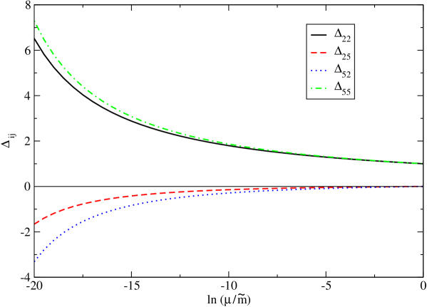
Figure 1: Renormalization group flow of $C^{\,\widetilde{\scriptscriptstyle H}}_{2}$ and $C^{\,\widetilde{\scriptscriptstyle H}}_{5}$, expressed in terms of the coefficients $\Delta_{ij}$ of eq. (40), for $\alpha_{s}(\widetilde{m})=0.05$ and $\alpha_{t}(\widetilde{m})=0.03$. The solid, dashed, dotted, and dot–dashed lines correspond to $\Delta_{22}$, $\Delta_{25}$, $\Delta_{52}$ and $\Delta_{55}$, respectively.

A computation of the ${\cal O}(\alpha_{s})$ part of the anomalous dimensions, restricted to the four–fermion operators, has been given in the appendix of ref. [5]. From the comparison with eq. (29) it appears that the authors of ref. [5] have omitted the mixing among the $B$–ino operators induced by the penguin diagrams. Also, we disagree with ref. [5] on the anomalous dimensions of the higgsino operators.

Once we have evolved the Wilson coefficients down to the renormalization scale at which we compute the gluino decay width, it is convenient to express the operators in terms of chargino and neutralino mass eigenstates. With the usual definitions for the chargino and neutralino mixing matrices $U$, $V$ and $N$, which we assume to be real, the $B$–ino, $W$–ino and higgsino spinors can be expressed as

$$\overline{\widetilde{W}^{+}}=\overline{\chi^{+}_{i}}\,\left(U_{i1}\,P_{L}+V_{i1}\,P_{R}\right),\;\;\;\;\;\;\overline{\widetilde{H}^{+}}=\overline{\chi^{+}_{i}}\,\left(U_{i2}\,P_{L}+V_{i2}\,P_{R}\right),$$ (41)

$$\overline{\widetilde{B}}=\overline{\chi^{0}_{i}}\,N_{i1}\,,\;\;\;\overline{\widetilde{W}^{3}}=\overline{\chi^{0}_{i}}\,N_{i2}\,,\;\;\;\overline{\widetilde{H}^{0}}=\overline{\chi^{0}_{i}}\,\left(N_{i4}\,P_{R}-N_{i3}\,P_{L}\right),$$ (42)

where $P_{L}$ and $P_{R}$ are the chiral projectors. In the basis of mass eigenstates, the effective Lagrangian becomes

$${\cal L}=\frac{1}{\widetilde{m}^{2}}\,\sum_{j}C^{\,{\chi}^{0}_{i}}_{j}\,Q^{\,{\chi}^{0}_{i}}_{j}\;+\;\frac{1}{\widetilde{m}^{2}}\,\left(\sum_{j}C^{\,{\chi}^{+}_{i}}_{j}\,Q^{\,{\chi}^{+}_{i}}_{j}+{\rm h.c.}\right).$$ (43)

The operators involving neutralinos and quarks and their corresponding Wilson coefficients are

$$Q^{\,{\chi}^{0}_{i}}_{1\,q_{\scriptscriptstyle L},q_{\scriptscriptstyle R}} = \overline{\chi^{0}_{i}}\,\gamma^{\mu}\,\gamma_{5}\,\,{\tilde{g}}^{a}\;\otimes\;\sum_{k=1}^{2}\,\overline{q}^{\,(k)}_{\scriptscriptstyle L,R}\,\gamma_{\mu}\,T^{a}\,q^{(k)}_{\scriptscriptstyle L,R}\hskip 56.9055pt(q=u,d)\,,$$ (44)

$$Q^{\,{\chi}^{0}_{i}}_{2\,q_{\scriptscriptstyle L},q_{\scriptscriptstyle R}} = \overline{\chi^{0}_{i}}\,\gamma^{\mu}\,\gamma_{5}\,{\tilde{g}}^{a}\;\otimes\;\overline{q}_{\scriptscriptstyle L,R}\,\gamma_{\mu}\,T^{a}\,q_{\scriptscriptstyle L,R}\hskip 78.24507pt(q=t,b)\,,$$ (45)

$$Q^{\,{\chi}^{0}_{i}}_{3\,q_{\scriptscriptstyle L},q_{\scriptscriptstyle R}} = \overline{\chi^{0}_{i}}_{\scriptscriptstyle R,L}\,{\tilde{g}}^{a}_{\scriptscriptstyle L,R}\;\otimes\;\overline{q}_{\scriptscriptstyle R,L}\,T^{a}\,q_{\scriptscriptstyle L,R}\hskip 98.16191pt(q=t,b)\,,$$ (46)

$$Q^{\,{\chi}^{0}_{i}}_{4\,q_{\scriptscriptstyle L},q_{\scriptscriptstyle R}} = \overline{\chi^{0}_{i}}_{\scriptscriptstyle R,L}\,\sigma^{\mu\nu}\,\gamma_{5}\,{\tilde{g}}^{a}_{\scriptscriptstyle L,R}\;\otimes\;\overline{q}_{\scriptscriptstyle R,L}\,\sigma_{\mu\nu}\,T^{a}\,q_{\scriptscriptstyle L,R}\hskip 46.94687pt(q=t,b)\,,$$ (47)

$$C^{\,{\chi}^{0}_{i}}_{1\,u_{\scriptscriptstyle L}}=C^{\,\widetilde{\scriptscriptstyle B}}_{1}\,N_{i1}+C^{\,\widetilde{\scriptscriptstyle W}}_{1}\,N_{i2}\,,\;\;\;\;\;C^{\,{\chi}^{0}_{i}}_{1\,u_{\scriptscriptstyle R}}=C^{\,\widetilde{\scriptscriptstyle B}}_{2}\,N_{i1}\,,$$ (48)

$$C^{\,{\chi}^{0}_{i}}_{1\,d_{\scriptscriptstyle L}}=C^{\,\widetilde{\scriptscriptstyle B}}_{1}\,N_{i1}-C^{\,\widetilde{\scriptscriptstyle W}}_{1}\,N_{i2}\,,\;\;\;\;\;C^{\,{\chi}^{0}_{i}}_{1\,d_{\scriptscriptstyle R}}=C^{\,\widetilde{\scriptscriptstyle B}}_{3}\,N_{i1}\,,$$ (49)

$$C^{\,{\chi}^{0}_{i}}_{2\,t_{\scriptscriptstyle L}}=C^{\,\widetilde{\scriptscriptstyle B}}_{4}\,N_{i1}+C^{\,\widetilde{\scriptscriptstyle W}}_{2}\,N_{i2}\,,\;\;\;\;C^{\,{\chi}^{0}_{i}}_{3\,t_{\scriptscriptstyle L}}=-C^{\,\widetilde{\scriptscriptstyle H}}_{1}\,N_{i4}\,,\;\;\;\;\;C^{\,{\chi}^{0}_{i}}_{4\,t_{\scriptscriptstyle L}}=C^{\,\widetilde{\scriptscriptstyle H}}_{2}\,N_{i4}\,,$$ (50)

$$C^{\,{\chi}^{0}_{i}}_{2\,t_{\scriptscriptstyle R}}=C^{\,\widetilde{\scriptscriptstyle B}}_{5}\,N_{i1}\,,\;\;\;\;\;C^{\,{\chi}^{0}_{i}}_{3\,t_{\scriptscriptstyle R}}=-C^{\,\widetilde{\scriptscriptstyle H}}_{1}\,N_{i4}\,,\;\;\;\;\;C^{\,{\chi}^{0}_{i}}_{4\,t_{\scriptscriptstyle R}}=-C^{\,\widetilde{\scriptscriptstyle H}}_{2}\,N_{i4}\,,$$ (51)

$$C^{\,{\chi}^{0}_{i}}_{2\,b_{\scriptscriptstyle L}}=C^{\,\widetilde{\scriptscriptstyle B}}_{4}\,N_{i1}-C^{\,\widetilde{\scriptscriptstyle W}}_{2}\,N_{i2}\;\;\;\;C^{\,{\chi}^{0}_{i}}_{3\,b_{\scriptscriptstyle L}}=-C^{\,\widetilde{\scriptscriptstyle H}}_{3}\,N_{i3}\,,\;\;\;\;\;C^{\,{\chi}^{0}_{i}}_{4\,b_{\scriptscriptstyle L}}=-C^{\,\widetilde{\scriptscriptstyle H}}_{4}\,N_{i3}\,,$$ (52)

$$C^{\,{\chi}^{0}_{i}}_{2\,b_{\scriptscriptstyle R}}=C^{\,\widetilde{\scriptscriptstyle B}}_{6}\,N_{i1}\,,\;\;\;\;\;C^{\,{\chi}^{0}_{i}}_{3\,b_{\scriptscriptstyle R}}=-C^{\,\widetilde{\scriptscriptstyle H}}_{3}\,N_{i3}\,,\;\;\;\;\;C^{\,{\chi}^{0}_{i}}_{4\,b_{\scriptscriptstyle R}}=C^{\,\widetilde{\scriptscriptstyle H}}_{4}\,N_{i3}.$$ (53)

The operators involving charginos and quarks and their Wilson coefficients are

$$Q^{\,{\chi}^{+}_{i}}_{1\,{\scriptscriptstyle L,R}} = \overline{\chi^{+}_{i}}_{\scriptscriptstyle L,R}\,\gamma^{\mu}\,{\tilde{g}}^{a}_{\scriptscriptstyle L,R}\;\otimes\;\sum_{k=1}^{2}\,\overline{d}_{\scriptscriptstyle L}^{\,(k)}\,\gamma_{\mu}\,T^{a}\,u_{\scriptscriptstyle L}^{(k)}$$ (54)

$$Q^{\,{\chi}^{+}_{i}}_{2\,{\scriptscriptstyle L,R}} = \overline{\chi^{+}_{i}}_{\scriptscriptstyle L,R}\,\gamma^{\mu}\,{\tilde{g}}^{a}_{\scriptscriptstyle L,R}\;\otimes\;\overline{b}_{\scriptscriptstyle L}\,\gamma_{\mu}\,T^{a}\,t_{\scriptscriptstyle L}$$ (55)

$$Q^{\,{\chi}^{+}_{i}}_{3\,{\scriptscriptstyle L,R}} = \overline{\chi^{+}_{i}}_{\scriptscriptstyle R,L}\,{\tilde{g}}^{a}_{\scriptscriptstyle L,R}\;\otimes\;\overline{b}_{\scriptscriptstyle R,L}\,T^{a}\,t_{\scriptscriptstyle L,R}$$ (56)

$$Q^{\,{\chi}^{+}_{i}}_{4\,{\scriptscriptstyle L,R}} = \overline{\chi^{+}_{i}}_{\scriptscriptstyle R,L}\,\sigma^{\mu\nu}\,{\tilde{g}}^{a}_{\scriptscriptstyle L,R}\;\otimes\;\overline{b}_{\scriptscriptstyle R,L}\,\sigma_{\mu\nu}\,T^{a}\,t_{\scriptscriptstyle L,R}$$ (57)

$$C^{\,{\chi}^{+}_{i}}_{1\,\scriptscriptstyle L}\;=\;-\sqrt{2}\,C^{\,\widetilde{\scriptscriptstyle W}}_{1}\,V_{i1}\,,\;\;\;\;\;C^{\,{\chi}^{+}_{i}}_{1\,\scriptscriptstyle R}\;=\;\sqrt{2}\,C^{\,\widetilde{\scriptscriptstyle W}}_{1}\,U_{i1}\,,$$ (58)

$$C^{\,{\chi}^{+}_{i}}_{2\,\scriptscriptstyle L}=-\sqrt{2}\,C^{\,\widetilde{\scriptscriptstyle W}}_{2}\,V_{i1}\,,\;\;\>C^{\,{\chi}^{+}_{i}}_{3\,\scriptscriptstyle L}=C^{\,\widetilde{\scriptscriptstyle H}}_{3}\,U_{i2}\,,\;\;\;\;\;C^{\,{\chi}^{+}_{i}}_{4\,\scriptscriptstyle L}=C^{\,\widetilde{\scriptscriptstyle H}}_{4}\,U_{i2}\,,$$ (59)

$$C^{\,{\chi}^{+}_{i}}_{2\,\scriptscriptstyle R}=\sqrt{2}\,C^{\,\widetilde{\scriptscriptstyle W}}_{2}\,U_{i1}\,,\;\;\;\;\;C^{\,{\chi}^{+}_{i}}_{3\,\scriptscriptstyle R}=C^{\,\widetilde{\scriptscriptstyle H}}_{1}\,V_{i2}\,,\;\;\;\;\;C^{\,{\chi}^{+}_{i}}_{4\,\scriptscriptstyle R}=C^{\,\widetilde{\scriptscriptstyle H}}_{2}\,V_{i2}\,.$$ (60)

All Wilson coefficients in eqs.(48)–(53) and (58)–(60) are evaluated at the scale $\mu$ at which the gluino decay width is computed (we take $\mu=m_{\tilde{g}}$ in our numerical analysis).

The magnetic operator involving a neutralino and a gluon is

$$Q^{\,{\chi}^{0}_{i}}_{g}=\overline{\chi^{0}_{i}}\,\sigma^{\mu\nu}\,\gamma_{5}\,{\tilde{g}}^{a}\,G_{\mu\nu}^{a}\,.$$ (61)

In order to reach the desired accuracy in the ${\tilde{g}}\to g{\tilde{\chi}}^{0}$ process, we need to include the matrix element contribution coming from the diagram in which the two top quarks in the operator $Q^{\,\widetilde{\scriptscriptstyle H}}_{2}$ close in a loop emitting a gluon. This results into an “effective” Wilson coefficient

$$\left.C^{\,{\chi}^{0}_{i}}_{g}\right._{\rm\!\!\!eff}(\mu)=C^{\,\widetilde{\scriptscriptstyle B}}_{7}(\mu)\,N_{i1}+C^{\,\widetilde{\scriptscriptstyle H}}_{5}(\mu)\,N_{i4}\,v+\frac{g_{s}\,h_{t}}{8\pi^{2}}\,C^{\,\widetilde{\scriptscriptstyle H}}_{2}(\mu)\,\,N_{i4}\,v\,\ln\frac{m_{t}^{2}}{\mu^{2}}\,,$$ (62)

where $v$ is the Higgs vacuum expectation value and we take $\mu=m_{\tilde{g}}$.

From the effective Lagrangian of eq. (43) we can compute the gluino decay widths and complete expressions can be found in the appendix. The same effective Lagrangian correctly describes also the interactions that lead to the decays ${\tilde{g}}\to gg{\tilde{\chi}}^{0}$ and ${\tilde{g}}\to gh^{0}{\tilde{\chi}}^{0}$. However, since these processes are subleading, we will not explicitly calculate their decay widths.

4 Results

We are now ready to discuss the results of our computation of the decay width and branching ratios of the gluino in Split Supersymmetry. The input parameters relevant to our analysis are the sfermion mass scale $\widetilde{m}$, the physical gluino mass $m_{\tilde{g}}$ and $\tan\beta$, which in Split Supersymmetry is interpreted as the tangent of the angle that rotates the finely tuned Higgs doublets. To simplify the analysis we assume that the squark masses are degenerate, i.e. we set $r_{\tilde{q}_{\scriptscriptstyle L}}=r_{\tilde{u}_{\scriptscriptstyle R}}=r_{\tilde{d}_{\scriptscriptstyle R}}=1$ in the matching conditions of the Wilson coefficients. The gluino mass parameter in the Lagrangian, $M_{3}$, is extracted from $m_{\tilde{g}}$ including radiative corrections, and the other gaugino masses $M_{1}$ and $M_{2}$ are computed from $M_{3}$ assuming unification at the GUT scale. The higgsino mass parameter $\mu$ is determined as a function of $M_{2}$ by requiring that the relic abundance of neutralinos is equal to the dark–matter density preferred by WMAP data [9] (see fig. 11 of ref. [2] ). The sign of $\mu$ remains a free parameter, but since it does not affect our results for the gluino decays in a significant way we will assume $\mu>0$ throughout our analysis. The effective couplings of gauginos and higgsinos at the weak scale, needed to compute the chargino and neutralino mass matrices, are determined from their high–energy (supersymmetric) boundary values by means of the renormalization–group equations of Split Supersymmetry, given in ref. [2]. Finally, the SM input parameters relevant to our analysis are: the physical masses for the top quark and gauge bosons, $m_{t}=178$ GeV, $M_{Z}=91.187$ GeV and $M_{W}=80.41$ GeV; the running bottom mass computed at the scale of the top mass, $m_{b}(m_{t})=2.75$ GeV; the Fermi constant, $G_{F}=1.166\times 10^{-5}$ GeV^-2; the running strong coupling computed at the scale of the top mass, $\alpha_{s}(m_{t})=0.106$.

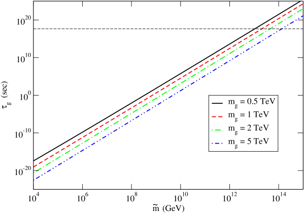
Figure 2: Gluino lifetime $\tau_{\tilde{g}}$ as a function of the sfermion mass scale $\widetilde{m}$, for different values of the physical gluino mass $m_{\tilde{g}}$. The other free parameters are chosen as $\tan\beta=2$ and $\mu>0$. The dashed horizontal line corresponds to the age of the universe, $\tau_{\scriptscriptstyle U}=14$ Gyr.

To start our discussion, we show in fig. 2 the gluino lifetime $\tau_{\tilde{g}}$ (in seconds) as a function of the sfermion mass scale $\widetilde{m}$, for $\tan\beta=2$ and four different values of the physical gluino mass ($m_{\tilde{g}}$ = 0.5, 1, 2 and 5 TeV, respectively). It can be seen that $\tau_{\tilde{g}}$ is about 4 seconds for $m_{\tilde{g}}=1$ TeV and $\widetilde{m}=10^{9}$ GeV. A value of $\tau_{\tilde{g}}$ equal to the age of the universe (14 Gyr) corresponds to $\widetilde{m}=(1.1,\,2.1,\,4.5,\,13)\times 10^{13}$ GeV for $m_{\tilde{g}}$ = 0.5, 1, 2 and 5 TeV, respectively.

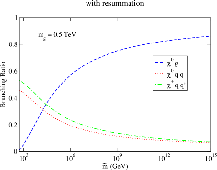
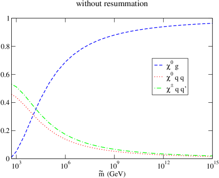
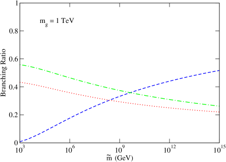
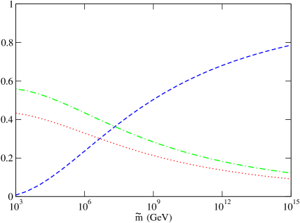
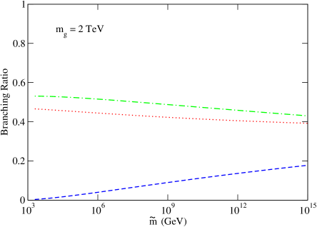
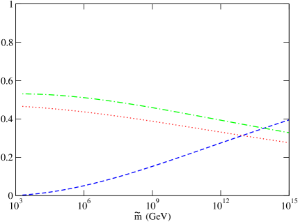
Figure 3: Branching ratios for the gluino decay channels $\chi^{0}g$ (dashed lines), $\chi^{0}q\bar{q}$ (dotted) and $\chi^{\pm}q\bar{q}^{\,\prime}$ (dot–dashed), summed over all possible neutralino or chargino states, as a function of $\widetilde{m}$, for three values of $m_{\tilde{g}}$: 500 GeV (upper plots), 1 TeV (middle) and 2 TeV (lower). The curves in the left (right) plots do (do not) include the resummation of the leading logarithmic corrections. Other parameters are $\tan\beta=20$ and $\mu>0$.

In fig. 3 we show the branching ratios for the three decay processes $\tilde{g}\rightarrow\chi^{0}g$, $\tilde{g}\rightarrow\chi^{0}q\bar{q}$ and $\tilde{g}\rightarrow\chi^{\pm}q\bar{q}^{\,\prime}$ (summed over all neutralino or chargino states) as a function of $\widetilde{m}$, for $\tan\beta=20$ and three different values of $m_{\tilde{g}}$ : 500 GeV (upper plots), 1 TeV (middle plots) and 2 TeV (lower plots). The value of $\tan\beta$ has little impact on these results. The plots on the left of fig. 3 represent the results of our full calculation, including the resummation of the leading logarithmic corrections controlled by $\alpha_{s}$ and $\alpha_{t}$. The plots on the right represent instead the lowest–order results that do not include the resummation. We obtain the latter results by replacing the Wilson coefficients of the four–fermion operators in the low–energy effective Lagrangian with their tree–level expressions in terms of gauge and Yukawa couplings [eqs. (9)–(10), (13) and (19)–(20)], and the Wilson coefficient of the magnetic operator with its one–loop expression. The plots in fig. 3 show that the branching ratio of the radiative decay $\tilde{g}\rightarrow\chi^{0}g$ decreases for increasing $m_{\tilde{g}}$ and increases for increasing $\widetilde{m}$. In fact, as stressed in ref. [7], the ratio between the two–body and three–body decay rates computed at lowest order scales like $m_{t}^{2}/m_{\tilde{g}}^{2}\;[1-\ln(\widetilde{m}^{2}/m_{t}^{2})]^{2}$, where the logarithmic term comes from the top–stop loop that generates the magnetic gluino–gluon–higgsino interaction. For large values of $\widetilde{m}$, the resummation of the logarithms becomes necessary. Comparing the plots on the left and right sides of fig. 3, we see that the resummation of the leading logarithmic corrections tends to enhance the three–body decays and suppress the radiative decay. The effect of the corrections on the branching ratios is particularly visible when, like in the middle and lower plots, neither the two–body nor the three–body channels are obviously dominant in the range $10^{8}$ GeV $<\widetilde{m}<10^{13}$ GeV, relevant to Split Supersymmetry.

       

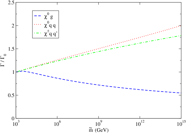
Figure 4: Effect of the radiative corrections on the partial widths for the decays $\tilde{g}\rightarrow\chi^{0}g$ (dashed lines), $\tilde{g}\rightarrow\chi^{0}q\bar{q}$ (dotted) and $\tilde{g}\rightarrow\chi^{\pm}q\bar{q}^{\,\prime}$ (dot–dashed) as a function of $\widetilde{m}$. The parameters are chosen as $m_{\tilde{g}}=1$ TeV, $\tan\beta=20$ and $\mu>0$.

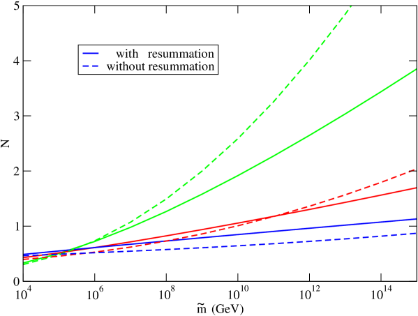
Figure 5: The normalization $N$ of eq. (63) as a function of the sfermion mass scale $\widetilde{m}$, with (solid lines) and without (dashed lines) resummation of the leading logarithmic corrections. The upper, middle and lower sets of curves correspond to $m_{\tilde{g}}=$ 0.5, 1 and 2 TeV, respectively. The other free parameters are chosen as $\tan\beta=20$ and $\mu>0$.

To further illustrate the effect of the resummation of the leading logarithmic corrections, we plot in fig. 4 the ratio $\Gamma/\Gamma_{0}$ of the partial decay widths with and without resummation, for the processes $\tilde{g}\rightarrow\chi^{0}g$, $\tilde{g}\rightarrow\chi^{0}q\bar{q}$ and $\tilde{g}\rightarrow\chi^{\pm}q\bar{q}^{\,\prime}$. We fix $m_{\tilde{g}}=1$ TeV, $\tan\beta=20$ and $\mu>0$, but we have checked that the qualitative behaviour of the corrections is independent of the precise choice of the parameters. It can be seen from fig. 4 that for large enough values of $\widetilde{m}$ the radiative corrections can be of the order of 50–100%, and that they enhance the widths for the three–body decays and suppress the width for the radiative decay.

To conclude this section, we discuss the scaling behaviour of the gluino lifetime and total decay width. The lifetime $\tau_{\tilde{g}}=\hbar/\Gamma_{\rm tot}$ can be written as

$$\tau_{\tilde{g}}=\frac{4\,{\rm sec}}{N}\,\times\,\left(\frac{\widetilde{m}}{10^{9}\,{\rm GeV}}\right)^{4}\times\left(\frac{1\,{\rm TeV}}{m_{\tilde{g}}}\right)^{5},$$ (63)

where the normalization $N$ is of order unity and depends on $\widetilde{m}$ and $m_{\tilde{g}}$ (and only very mildly on $\tan\beta$). In fig. 5 we show $N$ as a function of $\widetilde{m}$ for $\tan\beta=20$ and three different values of the physical gluino mass ($m_{\tilde{g}}=0.5,\,1$ and 2 TeV, respectively). The non–vanishing slope of $N$ represents the deviation of the total gluino decay width from the naive scaling behaviour $\Gamma_{\rm tot}\propto m_{\tilde{g}}^{5}\,/\,\widetilde{m}^{4}$. The solid lines in the plot represent the results of our full calculation, whereas the dashed lines represent the lowest–order results that do not include the resummation. For low values of $m_{\tilde{g}}$ the contribution of the radiative decay dominates (see fig. 3), thus the total decay width departs visibly from the naive scaling and is significantly suppressed by the resummation of the radiative corrections. On the other hand, for large values of $m_{\tilde{g}}$ the three–body decays dominate, and the effect of the resummation is to enhance the total decay width. Finally, for the intermediate value $m_{\tilde{g}}=1$ TeV there is a compensation between the corrections to the radiative decay width and those to the three–body decay widths, and the net effect on the total decay width of the resummation of the leading logarithmic corrections is rather small.

5 Gluino Decay into Gravitinos

Split Supersymmetry opens up the possibility of direct tree-level mediation of the original supersymmetry breaking to the SM superfields, without the need of a hidden sector [3]. In usual low-energy supersymmetry, this possibility is impracticable: for $F$–term breaking some scalars remain lighter than the SM matter fermions, and for $D$–term breaking gaugino masses cannot be generated at the same order of scalar masses. In Split Supersymmetry a large hierarchy between scalar and gaugino masses is acceptable, and indeed models have been proposed [3, 8] with direct mediation of $D$–term supersymmetry breaking.

Therefore, in Split Supersymmetry the original scale of supersymmetry breaking $\sqrt{F}$, which is related to the gravitino mass by

$$m_{3/2}=\sqrt{\frac{8\pi}{3}}\frac{F}{M_{\rm Pl}},$$ (64)

could be as low as the squark mass scale $\widetilde{m}$. This means that the interactions between the gluino and (the spin–1/2 component of) the gravitino, which are suppressed by $1/F$, could be as strong as those considered in the previous sections, which are suppressed by $1/\widetilde{m}^{2}$.

For $m_{3/2}\ll m_{\tilde{g}}$, the gravitino interactions can be obtained, through the supersymmetric analogue of the equivalence theorem [10], from the goldstino derivative coupling to the supercurrent. This approximation is valid as long as $\sqrt{F}\ll 6\times(m_{\tilde{g}}/1\,{\rm TeV})^{1/2}\times 10^{10}$ GeV. Using the equations of motion, we can write the effective goldstino ($\widetilde{G}$) interactions for on–shell particles as

$${\cal L}=\frac{1}{F}\left(-m_{{\tilde{q}}_{\scriptscriptstyle L}}^{2}{\tilde{q}}_{\scriptscriptstyle L}{\bar{q}}_{\scriptscriptstyle L}-m_{{\tilde{q}}_{\scriptscriptstyle R}}^{2}{\tilde{q}}_{\scriptscriptstyle R}{\bar{q}}_{\scriptscriptstyle R}+\frac{m_{\tilde{g}}}{4\sqrt{2}}\,{\overline{{\tilde{g}}^{a}}}\,\sigma^{\mu\nu}\gamma_{5}\,G^{a}_{\mu\nu}\right)\tilde{G}+{\rm h.c.}$$ (65)

Below $\widetilde{m}$, the effective Lagrangian describing the interactions between the gluino and the goldstino becomes

$${\cal L}=\frac{1}{F}\,\sum_{i=1}^{5}C^{\,\widetilde{\scriptscriptstyle G}}_{i}\,Q^{\,\widetilde{\scriptscriptstyle G}}_{i}\,,$$ (66)

$$Q^{\,\widetilde{\scriptscriptstyle G}}_{1} = \overline{\widetilde{G}}\,\gamma^{\mu}\,\gamma_{5}\,{\tilde{g}}^{a}\;\otimes\;\sum_{k=1,2\atop q=u,d}\;\overline{q}^{\,(k)}\,\gamma_{\mu}\,T^{a}\,q^{\,(k)}$$ (67)

$$Q^{\,\widetilde{\scriptscriptstyle G}}_{2} = \overline{\widetilde{G}}\,\gamma^{\mu}\,\gamma_{5}\,{\tilde{g}}^{a}\;\otimes\;\overline{q}_{\scriptscriptstyle L}^{\,(3)}\,\gamma_{\mu}\,T^{a}\,q_{\scriptscriptstyle L}^{\,(3)}$$ (68)

$$Q^{\,\widetilde{\scriptscriptstyle G}}_{3} = \overline{\widetilde{G}}\,\gamma^{\mu}\,\gamma_{5}\,{\tilde{g}}^{a}\;\otimes\;\overline{t}_{\scriptscriptstyle R}\,\gamma_{\mu}\,T^{a}\,t_{\scriptscriptstyle R}$$ (69)

$$Q^{\,\widetilde{\scriptscriptstyle G}}_{4} = \overline{\widetilde{G}}\,\gamma^{\mu}\,\gamma_{5}\,{\tilde{g}}^{a}\;\otimes\;\overline{b}_{\scriptscriptstyle R}\,\gamma_{\mu}\,T^{a}\,b_{\scriptscriptstyle R}$$ (70)

$$Q^{\,\widetilde{\scriptscriptstyle G}}_{5} = \overline{\widetilde{G}}\,\sigma^{\mu\nu}\,\gamma_{5}\,{\tilde{g}}^{a}\;G^{a}_{\mu\nu}.$$ (71)

The Wilson coefficients at the matching scale $\widetilde{m}$ are

$$C^{\,\widetilde{\scriptscriptstyle G}}_{1}=C^{\,\widetilde{\scriptscriptstyle G}}_{2}=C^{\,\widetilde{\scriptscriptstyle G}}_{3}=C^{\,\widetilde{\scriptscriptstyle G}}_{4}=-\frac{g_{s}}{\sqrt{2}}\,,\;\;\;\;\;\;\;C^{\,\widetilde{\scriptscriptstyle G}}_{5}=-\frac{m_{\tilde{g}}}{2\,\sqrt{2}}.$$ (72)

Note that the coefficients of the interactions in eq. (66) have no dependence on $\widetilde{m}$, because the squark mass square in the propagators of the particles we integrate out is exactly cancelled by the squark mass square in the goldstino coupling in eq. (65).

The operator renormalization proceeds analogously to the discussion in sect. 3. The anomalous dimension matrix of the operators in eqs. (67)–(71) is given by eq. (28) with

$$\gamma_{s}^{\widetilde{\scriptscriptstyle G}}=\frac{1}{3}\pmatrix{16-9N_{c}&16&16&16&0\cr 4&4-9N_{c}&4&4&0\cr 2&2&2-9N_{c}&2&0\cr 2&2&2&2-9N_{c}&0\cr 0&0&0&0&2N_{f}-18N_{c}},$$ (73)

$$\gamma_{t}^{\widetilde{\scriptscriptstyle G}}=\pmatrix{0&0&0&0&0\cr 0&1&\!\!\!\!-2&0&0\cr 0&\!\!\!\!-1&2&0&0\cr 0&0&0&0&0},~{}~{}~{}~{}\gamma_{st}^{\widetilde{\scriptscriptstyle G}}=0\,.$$ (74)

The evolution of the Wilson coefficients for the goldstino operators has the simple analytic form

$$C^{\,\widetilde{\scriptscriptstyle G}}_{i}(\mu) = \eta_{s}^{-\frac{9}{10}}\left[C^{\,\widetilde{\scriptscriptstyle G}}_{i}(\widetilde{m})+y\,{\overline{C}^{\,\widetilde{\scriptscriptstyle G}}}(\widetilde{m})\right]~{}~{}~{}i=1,4$$ (75)

$$C^{\,\widetilde{\scriptscriptstyle G}}_{2}(\mu) = \eta_{s}^{-\frac{9}{10}}\left[(1+z)\,C^{\,\widetilde{\scriptscriptstyle G}}_{2}(\widetilde{m})-z\,C^{\,\widetilde{\scriptscriptstyle G}}_{3}(\widetilde{m})+y\,{\overline{C}^{\,\widetilde{\scriptscriptstyle G}}}(\widetilde{m})\right],$$ (76)

$$C^{\,\widetilde{\scriptscriptstyle G}}_{3}(\mu) = \eta_{s}^{-\frac{9}{10}}\left[(1+2\,z)\,C^{\,\widetilde{\scriptscriptstyle G}}_{3}(\widetilde{m})-2\,z\,C^{\,\widetilde{\scriptscriptstyle G}}_{2}(\widetilde{m})+y\,{\overline{C}^{\,\widetilde{\scriptscriptstyle G}}}(\widetilde{m})\right],$$ (77)

$$C^{\,\widetilde{\scriptscriptstyle G}}_{5}(\mu) = \eta_{s}^{-\frac{7}{5}}\,C^{\,\widetilde{\scriptscriptstyle G}}_{5}(\widetilde{m})\,,$$ (78)

where ${\overline{C}^{\,\widetilde{\scriptscriptstyle G}}}=2\,C^{\,\widetilde{\scriptscriptstyle G}}_{1}/3+C^{\,\widetilde{\scriptscriptstyle G}}_{2}/6+(C^{\,\widetilde{\scriptscriptstyle G}}_{3}+C^{\,\widetilde{\scriptscriptstyle G}}_{4})/12$, $y=\eta_{s}^{\,4/5}-1$, and $z=(\eta_{s}^{\,8/15}\,\eta_{t}^{-1/3}-1)/3$. The quantities $\eta_{s}$ and $\eta_{t}$ have been defined in eqs. (35) and (36), respectively.

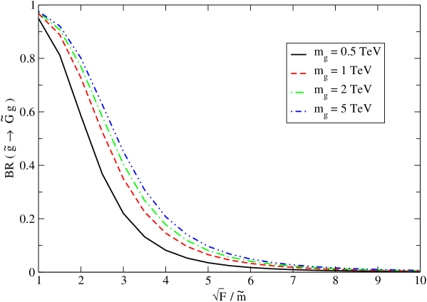
Figure 6: Branching ratio for the decay $\tilde{g}\rightarrow\widetilde{G}\,g$ as a function of $\sqrt{F}/\widetilde{m}$, for different values of the physical gluino mass $m_{\tilde{g}}$. The other free parameters are chosen as $\widetilde{m}=10^{9}$ GeV, $\tan\beta=2$ and $\mu>0$.

The formulae for the gluino decay widths into goldstino and quarks and into goldstino and gluon can be found in the appendix. In fig. 6 we show the branching ratio for the process $\tilde{g}\rightarrow\widetilde{G}\,g$ as a function of the ratio $\sqrt{F}/\widetilde{m}$, for $\widetilde{m}=10^{9}$ GeV, $\tan\beta=2\,,\;\mu>0$ and different values of the gluino mass. The branching ratio for the decay into goldstino and quarks, suppressed by phase space, is always at or below the 1% level. It can be seen from fig. 6 that the gluino decay into goldstino and gluon is largely dominant when $\sqrt{F}$ is as low as $\widetilde{m}$. In fact, the decays into charginos or neutralinos and quarks (relevant for large values of $m_{\tilde{g}}$) are suppressed by phase space, while the radiative decay into gluon and neutralinos (relevant for smaller values of $m_{\tilde{g}}$) is suppressed by $m_{t}^{2}/m_{\tilde{g}}^{2}$ and a loop factor. With respect to the scaling behaviour outlined in eq. (63), the additional contribution to the total gluino decay width coming from the decay into goldstino and gluon can significantly suppress the gluino lifetime. In fact, for $\sqrt{F}=\widetilde{m}$ the normalization $N$ in eq. (63) takes on values of order 40–50 for $\widetilde{m}>10^{8}$ GeV.

On the other hand, the widths for the gluino decays into goldstino are suppressed by a factor $\widetilde{m}^{4}/F^{2}$ with respect to those for decays into charginos or neutralinos. Fig. 6 shows that as soon as we depart from the condition $\sqrt{F}=\widetilde{m}$ the branching ratio for $\tilde{g}\rightarrow\widetilde{G}\,g$ falls off very quickly, and already for $\sqrt{F}/\widetilde{m}$ as large as 10 the gluino decays into goldstino are below the 1% level.

6 Conclusions

If Split Supersymmetry is the correct theory to describe physics beyond the Standard Model, one of its most spectacular manifestations might be the discovery of a very long–lived gluino at the LHC. In this paper we provided a precise determination of the gluino lifetime and branching ratios. Applying to Split Supersymmetry the effective Lagrangian and renormalization group techniques, we discussed the proper treatment of the radiative corrections that are enhanced by the large logarithm of the ratio between the sfermion mass scale and the gluino mass. We computed the anomalous dimensions of the operators relevant to the gluino decay, that allow us to resum to all orders in the perturbative expansion the leading logarithmic corrections controlled by $\alpha_{s}$ and $\alpha_{t}$. We also provided explicit analytical formulae for the gluino decay widths in terms of the Wilson coefficients of the effective Lagrangian of Split Supersymmetry. For representative values of the input parameters, we discussed the numerical impact of the radiative corrections and found that they can modify substantially the gluino decay width and branching ratios. Finally, we considered models with direct mediation of supersymmetry breaking, and we found that the gluino decays into gravitinos might dominate over the other decay modes.

Appendix

We present in this appendix the explicit formulae for the leading three–body and two–body gluino decay widths. All the results are expressed in terms of the Wilson coefficients of the effective Lagrangian of Split Supersymmetry, discussed in sects. 2, 3 and 5.

Three–body decays into quarks and chargino or neutralino:

denoting the momenta of the decay products as $(p_{1},p_{2},p_{3})\equiv(p_{q_{I}},p_{\overline{q}_{J}},p_{\chi})$, and $s_{ij}=(p_{i}+p_{j})^{2}$, the three–body decay amplitude is given by

$$\Gamma_{\chi\,q_{I}\overline{q}_{J}}=\frac{1}{256\,\pi^{3}\,m_{\tilde{g}}^{3}\;\widetilde{m}^{4}}\;\int\;\overline{\left|{\cal M}\right|^{2}}\;ds_{13}\,ds_{23}\,.$$ (79)

The bar over $\left|{\cal M}\right|^{2}$ denotes the average over colour and spin of the gluino and the sum over colour and spin of the final state particles (the dependence on $\widetilde{m}$ has been factored out). The limits of the integration in the ($s_{13},s_{23}$) plane are

$$s_{13}^{\rm max} = m_{q_{I}}^{2}+m_{\chi}^{2}+\frac{1}{2\,s_{23}}\,\left[(m_{\tilde{g}}^{2}-m_{q_{I}}^{2}-s_{23})\,(s_{23}-m_{\overline{q}_{J}}^{2}+m_{\chi}^{2})\right.$$ (80)

$$\hskip 113.81102pt+\left.\lambda^{1/2}(s_{23},m_{\tilde{g}}^{2},m_{q_{I}}^{2})\,\lambda^{1/2}(s_{23},m_{\overline{q}_{J}}^{2},m_{\chi}^{2})\right]\,,$$

$$s_{13}^{\rm min} = m_{q_{I}}^{2}+m_{\chi}^{2}+\frac{1}{2\,s_{23}}\,\left[(m_{\tilde{g}}^{2}-m_{q_{I}}^{2}-s_{23})\,(s_{23}-m_{\overline{q}_{J}}^{2}+m_{\chi}^{2})\right.$$ (81)

$$\hskip 113.81102pt-\left.\lambda^{1/2}(s_{23},m_{\tilde{g}}^{2},m_{q_{I}}^{2})\,\lambda^{1/2}(s_{23},m_{\overline{q}_{J}}^{2},m_{\chi}^{2})\right]\,,$$

$$s_{23}^{\rm max} = (|m_{\tilde{g}}|-m_{q_{I}})^{2}\,,$$ (82)

$$s_{23}^{\rm min} = (|m_{\chi}|+m_{\overline{q}_{J}})^{2}\,,$$ (83)

where $\lambda(x,y,z)=x^{2}+y^{2}+z^{2}-2\,(xy+xz+yz)$.

In the computation of the decays involving quarks of the first and second generation we can neglect the quark masses and we find

$$\Gamma_{\chi_{i}^{+}d\overline{u}}=\Gamma_{\chi_{i}^{-}u\overline{d}} = \frac{m_{\tilde{g}}^{5}}{1536\,\pi^{3}\,\widetilde{m}^{4}}\left[\left(\left.C^{\,{\chi}^{+}_{i}}_{1\,\scriptscriptstyle L}\right.^{2}+\left.C^{\,{\chi}^{+}_{i}}_{1\,\scriptscriptstyle R}\right.^{2}\right)\,g(x_{i})-2\,C^{\,{\chi}^{+}_{i}}_{1\,\scriptscriptstyle L}\,C^{\,{\chi}^{+}_{i}}_{1\,\scriptscriptstyle R}\,f(x_{i})\right]\,,$$ (84)

$$\Gamma_{\chi_{i}^{0}q\overline{q}} = \frac{m_{\tilde{g}}^{5}}{768\,\pi^{3}\,\widetilde{m}^{4}}\;\left(\left.C^{\,{\chi}^{0}_{i}}_{1\,q_{\scriptscriptstyle L}}\right.^{2}+\left.C^{\,{\chi}^{0}_{i}}_{1\,q_{\scriptscriptstyle R}}\right.^{2}\,\right)\,\biggr{[}g(x_{i})+f(x_{i})\biggr{]}\;\;\;\;(q=u,d)\,,$$ (85)

where $x_{i}=m_{\chi_{i}}/m_{\tilde{g}}$, and we have included an overall factor 2 to take into account the sum over the two generations of light quarks. The functions $f$ and $g$ are defined as:

$$g(x) = 1-8\,x^{2}+8\,x^{6}-x^{8}-12\,x^{4}\,\ln x^{2}\,,$$ (86)

$$f(x) = 2\,x+18\,x^{3}-18\,x^{5}-2\,x^{7}+12\,x^{3}(1+x^{2})\,\ln x^{2}\,.$$ (87)

For generic quark masses the integration of the squared amplitude $\overline{\left|{\cal M}\right|^{2}}$ on the $(s_{13},s_{23})$ plane cannot be performed analytically, and in order to compute the total decay width we must resort to a numerical integration.

The squared amplitude for the processes $\tilde{g}\rightarrow\chi_{i}^{+}\,b\,\overline{t}$ and $\tilde{g}\rightarrow\chi_{i}^{-}\,t\,\overline{b}$ is given by

$$\overline{\left|{\cal M}\right|^{2}} = \left.C^{\,{\chi}^{+}_{i}}_{2\,\scriptscriptstyle L}\right.^{2}\,(m_{\tilde{g}}^{2}+m_{t}^{2}-s_{13})\,(s_{13}-m_{\chi^{+}_{i}}^{2}-m_{b}^{2})$$ (88)

$$+ \left.C^{\,{\chi}^{+}_{i}}_{2\,\scriptscriptstyle R}\right.^{2}\,(m_{\tilde{g}}^{2}+m_{b}^{2}-s_{23})\,(s_{23}-m_{\chi^{+}_{i}}^{2}-m_{t}^{2})$$

$$+ \frac{1}{4}\,\left(\left.C^{\,{\chi}^{+}_{i}}_{3\,\scriptscriptstyle L}\right.^{2}+\left.C^{\,{\chi}^{+}_{i}}_{3\,\scriptscriptstyle R}\right.^{2}\right)\;(m_{\chi^{+}_{i}}^{2}+m_{\tilde{g}}^{2}-s_{13}-s_{23})\,(s_{13}+s_{23}-m_{t}^{2}-m_{b}^{2})$$

$$+ 4\,\left(\left.C^{\,{\chi}^{+}_{i}}_{4\,\scriptscriptstyle L}\right.^{2}+\left.C^{\,{\chi}^{+}_{i}}_{4\,\scriptscriptstyle R}\right.^{2}\right)\;\biggr{[}(m_{\chi^{+}_{i}}^{2}+m_{\tilde{g}}^{2}-s_{13}-s_{23})\,(s_{13}+s_{23}-m_{t}^{2}-m_{b}^{2}-4\,m_{\chi^{+}_{i}}^{2})$$

$$\hskip 113.81102pt+4\,(s_{13}-m_{\chi^{+}_{i}}^{2})\,(s_{23}-m_{\chi^{+}_{i}}^{2})-4\,m_{t}^{2}\,m_{b}^{2}\biggr{]}$$

$$+ 2\,C^{\,{\chi}^{+}_{i}}_{2\,\scriptscriptstyle L}\,C^{\,{\chi}^{+}_{i}}_{2\,\scriptscriptstyle R}\,m_{\tilde{g}}\,m_{\chi^{+}_{i}}\,(s_{13}+s_{23}-m_{\chi^{+}_{i}}^{2}-m_{\tilde{g}}^{2})$$

$$+ \left(C^{\,{\chi}^{+}_{i}}_{2\,\scriptscriptstyle R}\,C^{\,{\chi}^{+}_{i}}_{3\,\scriptscriptstyle R}+12\,C^{\,{\chi}^{+}_{i}}_{2\,\scriptscriptstyle R}\,C^{\,{\chi}^{+}_{i}}_{4\,\scriptscriptstyle R}\right)\,m_{\chi^{+}_{i}}\,m_{t}\,(s_{23}-m_{b}^{2}-m_{\tilde{g}}^{2})$$

$$+ \left(C^{\,{\chi}^{+}_{i}}_{2\,\scriptscriptstyle R}\,C^{\,{\chi}^{+}_{i}}_{3\,\scriptscriptstyle L}+12\,C^{\,{\chi}^{+}_{i}}_{2\,\scriptscriptstyle R}\,C^{\,{\chi}^{+}_{i}}_{4\,\scriptscriptstyle L}\right)\,m_{\tilde{g}}\,m_{b}\,(s_{23}-m_{t}^{2}-m_{\chi^{+}_{i}}^{2})$$

$$- \left(C^{\,{\chi}^{+}_{i}}_{2\,\scriptscriptstyle L}\,C^{\,{\chi}^{+}_{i}}_{3\,\scriptscriptstyle R}-12\,C^{\,{\chi}^{+}_{i}}_{2\,\scriptscriptstyle L}\,C^{\,{\chi}^{+}_{i}}_{4\,\scriptscriptstyle R}\right)\,m_{\tilde{g}}\,m_{t}\,(s_{13}-m_{b}^{2}-m_{\chi^{+}_{i}}^{2})$$

$$- \left(C^{\,{\chi}^{+}_{i}}_{2\,\scriptscriptstyle L}\,C^{\,{\chi}^{+}_{i}}_{3\,\scriptscriptstyle L}-12\,C^{\,{\chi}^{+}_{i}}_{2\,\scriptscriptstyle L}\,C^{\,{\chi}^{+}_{i}}_{4\,\scriptscriptstyle L}\right)\,m_{\chi^{+}_{i}}\,m_{b}\,(s_{13}-m_{t}^{2}-m_{\tilde{g}}^{2})$$

$$+ 2\,\left(C^{\,{\chi}^{+}_{i}}_{3\,\scriptscriptstyle L}\,C^{\,{\chi}^{+}_{i}}_{4\,\scriptscriptstyle L}+C^{\,{\chi}^{+}_{i}}_{3\,\scriptscriptstyle R}\,C^{\,{\chi}^{+}_{i}}_{4\,\scriptscriptstyle R}\right)\,\left[(m_{\tilde{g}}^{2}+m_{\chi^{+}_{i}}^{2}-s_{13}-s_{23})\,(s_{23}-s_{13}+m_{b}^{2}-m_{t}^{2})\right.$$

$$\hskip 113.81102pt\left.+2\,m_{b}^{2}\,(s_{23}-m_{t}^{2}-m_{\chi^{+}_{i}}^{2})-2\,m_{t}^{2}\,(s_{13}-m_{b}^{2}-m_{\chi^{+}_{i}}^{2})\right]$$

$$- 2\,\left(C^{\,{\chi}^{+}_{i}}_{3\,\scriptscriptstyle L}\,C^{\,{\chi}^{+}_{i}}_{3\,\scriptscriptstyle R}+48\,C^{\,{\chi}^{+}_{i}}_{4\,\scriptscriptstyle L}\,C^{\,{\chi}^{+}_{i}}_{4\,\scriptscriptstyle R}\right)\,m_{\tilde{g}}\,m_{\chi^{+}_{i}}\,m_{t}\,m_{b}\;.$$

The squared amplitude for the processes $\tilde{g}\rightarrow\chi_{i}^{0}\,t\,\overline{t}$ and $\tilde{g}\rightarrow\chi_{i}^{0}\,b\,\overline{b}$ is given by

$$\overline{\left|{\cal M}\right|^{2}} = \left(\left.C^{\,{\chi}^{0}_{i}}_{2\,q_{\scriptscriptstyle L}}\right.^{2}+\left.C^{\,{\chi}^{0}_{i}}_{2\,q_{\scriptscriptstyle R}}\right.^{2}\,\right)\;\left[(m_{\tilde{g}}^{2}+m_{q}^{2}-s_{13})\,(s_{13}-m_{q}^{2}-m_{\chi^{0}_{i}}^{2})\right.$$ (89)

$$\hskip 28.45274pt\left.+\,(m_{\tilde{g}}^{2}+m_{q}^{2}-s_{23})\,(s_{23}-m_{q}^{2}-m_{\chi^{0}_{i}}^{2})+2\,m_{\tilde{g}}\,m_{\chi^{0}_{i}}\,(m_{\tilde{g}}^{2}+m_{\chi^{0}_{i}}^{2}-s_{13}-s_{23})\right]$$

$$+ \frac{1}{4}\,\left(\left.C^{\,{\chi}^{0}_{i}}_{3\,q_{\scriptscriptstyle L}}\right.^{2}+\left.C^{\,{\chi}^{0}_{i}}_{3\,q_{\scriptscriptstyle R}}\right.^{2}\,\right)\,(m_{\chi^{0}_{i}}^{2}+m_{\tilde{g}}^{2}-s_{13}-s_{23})(s_{13}+s_{23}-2\,m_{q}^{2})$$

$$+ 4\,\left(\left.C^{\,{\chi}^{0}_{i}}_{4\,q_{\scriptscriptstyle L}}\right.^{2}+\left.C^{\,{\chi}^{0}_{i}}_{4\,q_{\scriptscriptstyle R}}\right.^{2}\,\right)\,\left[(m_{\chi^{0}_{i}}^{2}+m_{\tilde{g}}^{2}+4\,m_{q}^{2}-s_{13}-s_{23})(s_{13}+s_{23}-2\,m_{q}^{2}-4\,m_{\chi^{0}_{i}}^{2})\right.$$

$$\hskip 113.81102pt\left.+4\,(s_{13}-m_{q}^{2}-m_{\chi^{0}_{i}}^{2})\,(s_{23}-m_{q}^{2}-m_{\chi^{0}_{i}}^{2})+8\,m_{q}^{2}\,m_{\chi^{0}_{i}}^{2})\right]$$

$$+ 4\,C^{\,{\chi}^{0}_{i}}_{2\,q_{\scriptscriptstyle L}}\,C^{\,{\chi}^{0}_{i}}_{2\,q_{\scriptscriptstyle R}}\,m_{q}^{2}\,(s_{13}+s_{23}+4\,m_{\tilde{g}}\,m_{\chi^{0}_{i}}-2\,m_{q}^{2})$$

$$+ \left(C^{\,{\chi}^{0}_{i}}_{2\,q_{\scriptscriptstyle R}}\,C^{\,{\chi}^{0}_{i}}_{3\,q_{\scriptscriptstyle R}}-C^{\,{\chi}^{0}_{i}}_{2\,q_{\scriptscriptstyle L}}\,C^{\,{\chi}^{0}_{i}}_{3\,q_{\scriptscriptstyle L}}\right)\,m_{q}\,\left[m_{\chi^{0}_{i}}\,(m_{\tilde{g}}^{2}+m_{q}^{2}-s_{13})+m_{\tilde{g}}\,(m_{\chi^{0}_{i}}^{2}+m_{q}^{2}-s_{23})\right]$$

$$+ \left(C^{\,{\chi}^{0}_{i}}_{2\,q_{\scriptscriptstyle R}}\,C^{\,{\chi}^{0}_{i}}_{3\,q_{\scriptscriptstyle L}}-C^{\,{\chi}^{0}_{i}}_{2\,q_{\scriptscriptstyle L}}\,C^{\,{\chi}^{0}_{i}}_{3\,q_{\scriptscriptstyle R}}\right)\,m_{q}\,\left[m_{\chi^{0}_{i}}\,(m_{\tilde{g}}^{2}+m_{q}^{2}-s_{23})+m_{\tilde{g}}\,(m_{\chi^{0}_{i}}^{2}+m_{q}^{2}-s_{13})\right]$$

$$+ 12\,\left(C^{\,{\chi}^{0}_{i}}_{2\,q_{\scriptscriptstyle R}}\,C^{\,{\chi}^{0}_{i}}_{4\,q_{\scriptscriptstyle R}}-C^{\,{\chi}^{0}_{i}}_{2\,q_{\scriptscriptstyle L}}\,C^{\,{\chi}^{0}_{i}}_{4\,q_{\scriptscriptstyle L}}\right)\,m_{q}\,\left[m_{\tilde{g}}\,(m_{\chi^{0}_{i}}^{2}+m_{q}^{2}-s_{23})-m_{\chi^{0}_{i}}\,(m_{\tilde{g}}^{2}+m_{q}^{2}-s_{13})\right]$$

$$+ 12\,\left(C^{\,{\chi}^{0}_{i}}_{2\,q_{\scriptscriptstyle R}}\,C^{\,{\chi}^{0}_{i}}_{4\,q_{\scriptscriptstyle L}}-C^{\,{\chi}^{0}_{i}}_{2\,q_{\scriptscriptstyle L}}\,C^{\,{\chi}^{0}_{i}}_{4\,q_{\scriptscriptstyle R}}\right)\,m_{q}\,\left[m_{\chi^{0}_{i}}\,(m_{\tilde{g}}^{2}+m_{q}^{2}-s_{13})-m_{\tilde{g}}\,(m_{\chi^{0}_{i}}^{2}+m_{q}^{2}-s_{23})\right]$$

$$+ 2\,\left(C^{\,{\chi}^{0}_{i}}_{3\,q_{\scriptscriptstyle L}}\,C^{\,{\chi}^{0}_{i}}_{4\,q_{\scriptscriptstyle L}}+C^{\,{\chi}^{0}_{i}}_{3\,q_{\scriptscriptstyle R}}\,C^{\,{\chi}^{0}_{i}}_{4\,q_{\scriptscriptstyle R}}\right)\,(m_{\tilde{g}}^{2}+m_{\chi^{0}_{i}}^{2}+2\,m_{q}^{2}-s_{13}-s_{23})\,(s_{23}-s_{13})$$

$$- 2\,\left(C^{\,{\chi}^{0}_{i}}_{3\,q_{\scriptscriptstyle L}}\,C^{\,{\chi}^{0}_{i}}_{3\,q_{\scriptscriptstyle R}}+48\,C^{\,{\chi}^{0}_{i}}_{4\,q_{\scriptscriptstyle L}}\,C^{\,{\chi}^{0}_{i}}_{4\,q_{\scriptscriptstyle R}}\right)\,m_{\tilde{g}}\,m_{\chi^{0}_{i}}\,m_{q}^{2}\;\;\;\;\;\;\;\;\;\;\;\;(q=t,b).$$

We have checked that inserting in eqs. (88)–(89) the high–energy (i.e. non resummed) expressions for the Wilson coefficients given in sects. 2 and 3 we reproduce the tree–level results of ref. [7].

Two–body decays into neutralino and gluon:

the width for the radiative decay of the gluino, $\tilde{g}\rightarrow g\,\chi_{i}^{0}$, is

$$\Gamma_{\chi^{0}_{i}g}=\frac{(m_{\tilde{g}}^{2}-m_{\chi^{0}_{i}}^{2})^{3}}{2\,\pi\,m_{\tilde{g}}^{3}\,\widetilde{m}^{4}}\,\left(\left.C^{\,{\chi}^{0}_{i}}_{g}\right._{\rm\!\!\!eff}\right)^{2}\,.$$ (90)

The use of the effective coefficient $\left.C^{\,{\chi}^{0}_{i}}_{g}\right._{\rm\!\!\!eff}$ defined in eq. (62) allows us to reproduce the complete one–loop result when the resummation is switched off.

Decays into goldstino:

the decay width into goldstino and quarks of the first and second generation is:

$$\Gamma_{\widetilde{G}\overline{q}q}=\frac{m_{\tilde{g}}^{5}}{192\,\pi^{3}\,F^{2}}\;\left.C^{\,\widetilde{\scriptscriptstyle G}}_{1}\right.^{\,2}\,,$$ (91)

where we have summed over all four light quark flavours.

The gluino decay width into goldstino and third–generation quarks is as in eq. (79), with $\widetilde{m}^{4}$ replaced by $F^{2}$. The squared decay amplitude, which has to be integrated numerically on the $(s_{13},s_{23})$ plane, is given by

$$\overline{\left|{\cal M}\right|^{2}} = \left(\left.C^{\,\widetilde{\scriptscriptstyle G}}_{q_{\scriptscriptstyle L}}\right.^{2}+\left.C^{\,\widetilde{\scriptscriptstyle G}}_{q_{\scriptscriptstyle R}}\right.^{2}\right)\;\left[(m_{\tilde{g}}^{2}+m_{q}^{2}-s_{13})\,(s_{13}-m_{q}^{2})+\,(m_{\tilde{g}}^{2}+m_{q}^{2}-s_{23})\,(s_{23}-m_{q}^{2})\right]$$ (92)

$$+ 4\,C^{\,\widetilde{\scriptscriptstyle G}}_{q_{\scriptscriptstyle L}}\,C^{\,\widetilde{\scriptscriptstyle G}}_{q_{\scriptscriptstyle R}}\,m_{q}^{2}\,(s_{13}+s_{23}-2\,m_{q}^{2})\;\;\;\;\;\;\;\;\;\;\;\;\;(q=t,b)\,,$$

where

$$C^{\,\widetilde{\scriptscriptstyle G}}_{t_{\scriptscriptstyle L}}=C^{\,\widetilde{\scriptscriptstyle G}}_{b_{\scriptscriptstyle L}}=C^{\,\widetilde{\scriptscriptstyle G}}_{2}\,,\;\;\;\;\;\;\;C^{\,\widetilde{\scriptscriptstyle G}}_{t_{\scriptscriptstyle R}}=C^{\,\widetilde{\scriptscriptstyle G}}_{3}\,,\;\;\;\;\;\;\;C^{\,\widetilde{\scriptscriptstyle G}}_{b_{\scriptscriptstyle R}}=C^{\,\widetilde{\scriptscriptstyle G}}_{4}\,.$$ (93)

Finally, the gluino decay width into gluon and goldstino is:

$$\Gamma_{\widetilde{G}g}=\frac{m_{\tilde{g}}^{3}}{2\,\pi\,F^{2}}\,\left.C^{\,\widetilde{\scriptscriptstyle G}}_{5}\right.^{\,2}\,\;.$$ (94)

References

- [1] N. Arkani-Hamed and S. Dimopoulos, arXiv:hep-th/0405159.
- [2] G. F. Giudice and A. Romanino, Nucl. Phys. B 699 (2004) 65 [Erratum-ibid. B 706 (2005) 65] [arXiv:hep-ph/0406088].
- [3] N. Arkani-Hamed, S. Dimopoulos, G. F. Giudice and A. Romanino, Nucl. Phys. B 709 (2005) 3 [arXiv:hep-ph/0409232].
- [4] W. Kilian, T. Plehn, P. Richardson and E. Schmidt, Eur. Phys. J. C 39 (2005) 229 [arXiv:hep-ph/0408088]; J. L. Hewett, B. Lillie, M. Masip and T. G. Rizzo, JHEP 0409 (2004) 070 [arXiv:hep-ph/0408248]; L. Anchordoqui, H. Goldberg and C. Nunez, Phys. Rev. D 71 (2005) 065014 [arXiv:hep-ph/0408284]; K. Cheung and W. Y. Keung, Phys. Rev. D 71 (2005) 015015 [arXiv:hep-ph/0408335]; J. G. Gonzalez, S. Reucroft and J. Swain, arXiv:hep-ph/0504260.
- [5] A. Arvanitaki, C. Davis, P. W. Graham, A. Pierce and J. G. Wacker, arXiv:hep-ph/0504210.
- [6] H. E. Haber and G. L. Kane, Nucl. Phys. B 232 (1984) 333; H. Baer, V. D. Barger, D. Karatas and X. Tata, Phys. Rev. D 36 (1987) 96; R. Barbieri, G. Gamberini, G. F. Giudice and G. Ridolfi, Nucl. Phys. B 301 (1988) 15; H. Baer, X. Tata and J. Woodside, Phys. Rev. D 42 (1990) 1568; A. Bartl, W. Majerotto and W. Porod, Z. Phys. C 64 (1994) 499 [Erratum-ibid. C 68 (1995) 518]; A. Djouadi and Y. Mambrini, Phys. Lett. B 493 (2000) 120 [arXiv:hep-ph/0007174].
- [7] M. Toharia and J. D. Wells, arXiv:hep-ph/0503175.
- [8] K. S. Babu, T. Enkhbat and B. Mukhopadhyaya, arXiv:hep-ph/0501079.
- [9] C. L. Bennett et al., Astrophys. J. Suppl. 148 (2003) 1 [arXiv:astro-ph/0302207]; D. N. Spergel et al. [WMAP Collaboration], Astrophys. J. Suppl. 148 (2003) 175 [arXiv:astro-ph/0302209].
- [10] P. Fayet, Phys. Lett. B 70 (1977) 461; P. Fayet, Phys. Lett. B 86 (1979) 272; R. Casalbuoni, S. De Curtis, D. Dominici, F. Feruglio and R. Gatto, Phys. Rev. D 39 (1989) 2281.