Analytic evaluation of the amplitudes for orthopositronium decay to three photons to one-loop order

Abstract

The matrix element for the decay of orthopositronium to three photons can be expressed in terms of three independent amplitudes. We describe the analytic evaluation of these amplitudes, both to lowest order and with the inclusion of all one-loop corrections. We use these amplitudes to find precise values for the one-loop correction to the orthopositronium decay rate $\Gamma_{1}=-10.286606(10)(\alpha/\pi)\Gamma_{\rm LO}$, and for the order-$\alpha^{2}$ “square” correction to the decay rate $\Gamma_{2}({\rm square})=28.860(2)(\alpha/\pi)^{2}\Gamma_{\rm LO}$, where $\Gamma_{\rm LO}$ is the lowest order rate. We give in explicit form the function describing the one-loop correction to the distribution in phase space of the final state photons.

I Introduction

Positronium, the electron-positron bound state, is well-suited for probing many fundamental aspects of particle physics. Karshenboim04 The physics of positronium is governed almost exclusively by the electromagnetic force—weak interaction effects are negligible compared to present experimental and theoretical uncertainties Bernreuther81 ; Alcorta94 ; Govaerts96 ; Czarnecki99 . As a consequence, positronium is an ideal system for testing QED through high precision comparison between experimental and theoretical results for energy levels and decay rates. The states of positronium are eigenstates of the charge conjugation and parity operators C and P, so positronium can be used to test the discrete symmetries C, P, and T and combinations thereof. Vetter04 Positronium has been the focus of many past and ongoing attempts to observe physics beyond the standard model. Gninenko02 ; Rubbia04 In this work we focus on the decay of spin-1 orthopositronium to three photons.

The orthopositronium decay rate has been the subject of continuing experimental and theoretical work since the first measurement by Deutsch in 1951. Deutsch51 A summary of all experimental and theoretical results has been given by Adkins, Fell, and Sapirstein Adkins02 and updated with commentary by Rubbia Rubbia04 and by Sillou Sillou04 . By 1990 it was apparent that there was an “orthopositronium lifetime puzzle”, as the most precise experimental determinations (gas Westbrook89 and vacuum Nico90 results from the Michigan group) were in disagreement with theory Caswell77 ; Caswell79 by several standard deviations. Many experiments were mounted to look for exotic decays of orthopositronium in an attempt to resolve the discrepancy. Rubbia04 ; Dobroliubov93 ; Dvoeglazov93 ; Skalsey97 ; Vetter04a Newer, somewhat less precise powder results from the Tokyo group in 1995 Asai95 and 2000 Jinnouchi00 were consistent with theory and inconsistent with the earlier Michigan results. In 2000 the calculation of all $O(\alpha^{2})$ corrections to the decay rate were completed. Adkins00 ; Adkins02 Including yet higher order logarithmic corrections as well, Hill00 ; Kniehl00 ; Melnikov00 the theoretical prediction is Adkins02

$$\Gamma({\rm theory})=7.039979(11)\mu s^{-1}\,.$$ (1)

The $O(\alpha^{2})$ correction was found to be not unusually large, leaving the discrepancy with the Michigan results intact. Finally, in 2003 the lifetime puzzle was resolved by two new high-precision results from the Tokyo Jinnouchi03 and Michigan Vallery03 groups:

$$\Gamma({\rm Tokyo}) = 7.0396(12{\rm\,stat.})(11{\rm\,syst.})\mu s^{-1}$$ (2a)

$$\Gamma({\rm Michigan}) = 7.0404(10{\rm\,stat.})(8{\rm\,syst.})\mu s^{-1}\,,$$ (2b)

consistent with each other and with theory.

The resolution of the o-Ps lifetime puzzle does not decrease the long-term usefulness of positronium decay as a probe of fundamental physics. Ongoing and proposed experiments involving positronium decay include those of Refs. Vallery03 ; Crivelli04 ; Rubbia04 ; Gninenko04 ; Vetter04 . One challenge is to improve the experimental precision of the o-Ps decay rate (currently about 200 ppm) to a level closer to the present theoretical value (about 2 ppm). The $O(\alpha^{2})$ contribution to that rate is 250 ppm, so improved experimental precision will be required in order to test the $O(\alpha^{2})$ calculated result.

In this work we describe an analytic evaluation of the one-loop o-Ps$\rightarrow 3\gamma$ decay amplitudes. We use these amplitudes to obtain a precise value for the $O(\alpha)$ decay rate contribution, and also to calculate the part of the $O(\alpha^{2})$ correction coming from the square of the one-loop amplitudes. These results have been reported already Adkins96 —here we give further details. We also supply an explicit analytic expression for the $O(\alpha)$ differential decay rate in terms of photon energy variables. From the differential decay rate it is easy to obtain the $O(\alpha)$ corrected one-photon energy spectrum. (This energy spectrum, calculated more laboriously by numerical methods, has been useful in developing simulations of experimental arrangements. Asai95 ; Jinnouchi03 )

We adapt the formalism of covariant decay amplitudes, originally developed for the study of Z boson decay to three photons, Glover93 to the case of o-Ps$\rightarrow 3\gamma$. In Sec. II we use the extensive symmetries of the decay tensor to show that there are only three independent amplitudes for the o-Ps$\rightarrow 3\gamma$ decay. In Sec. III we express the decay amplitudes in terms of helicity variables since the spin sums are most convenient in this form. In Sec. IV the integral for the decay rate is reduced to its minimal two-dimensional form. In Sec. V the preceeding formalism is applied to the lowest-order decay process and the lowest-order decay rate of Ore and Powell Ore49 is reproduced. In Sec. VI the method of Passarino and Veltman Passarino79 for evaluating one-loop integrals is developed. In Sec. VII the one-loop calculation is described. Finally, in Sec. VIII our results for the $O(\alpha)$ and part of the $O(\alpha^{2})$ decay rates are given. The Appendix contains our explicit form for the one-loop decay distribution.

II Symmetries of the decay tensor

The decay of the massive vector particle orthopositronium to three photons is described by the matrix element conventions

$$M=\epsilon^{*}_{1\mu_{1}}\,\epsilon^{*}_{2\mu_{2}}\,\epsilon^{*}_{3\mu_{3}}\,\epsilon_{\alpha}\,M^{\mu_{1}\mu_{2}\mu_{3}\alpha}(k_{1},k_{2},k_{3})\quad,$$ (3)

where the three photons have momenta $k_{i}$ and polarizations $\epsilon_{i}$, and the positronium atom has momentum $P=k_{1}+k_{2}+k_{3}$ and polarization $\epsilon$. The decay tensor is a linear combination of terms like $k^{\mu_{1}}_{a}k^{\mu_{2}}_{b}k^{\mu_{3}}_{c}k^{\alpha}_{d}$, $k^{\mu_{1}}_{a}k^{\mu_{2}}_{b}g^{\mu_{3}\alpha}$, and $g^{\mu_{1}\mu_{2}}g^{\mu_{3}\alpha}$. The most general such tensor has 81 terms of the first type, 54 of the second, and 3 of the third. However, gauge invariance and Bose symmetry reduce the number of independent contributions to only three Glover93 . We review the argument below.

Because the decay tensor is always contracted with physical polarization vectors of on-shell photons, which satisfy $\epsilon_{a\mu}k^{\mu}_{a}=0$ (for $a=1$, 2, or 3), we can drop terms containing factors of $k^{\mu_{1}}_{1}$, $k^{\mu_{2}}_{2}$, and $k^{\mu_{3}}_{3}$. This leaves only 24 terms of the first type, 30 of the second, and still 3 of the third.

By Bose symmetry, the tensor $M$ is totally symmetric under photon interchange. This means, for the interchange of photons 1 and 2, that

$$M^{\mu_{1}\mu_{2}\mu_{3}\alpha}(k_{1},k_{2},k_{3})=M^{\mu_{2}\mu_{1}\mu_{3}\alpha}(k_{2},k_{1},k_{3})\quad.$$ (4)

This symmetry leaves only four independent terms of the first type, six of the second, and one of the third. The decay tensor can be written in the manifestly symmetric way

$$M^{\mu_{1}\mu_{2}\mu_{3}\alpha}(k_{1},k_{2},k_{3})=\sum_{S_{3}}{\cal M}^{\mu_{1}\mu_{2}\mu_{3}\alpha}(k_{1},k_{2},k_{3})\quad,$$ (5)

where the sum is over the six photon permutations, and the tensor $\cal M$ has the form

$${\cal M}^{\mu_{1}\mu_{2}\mu_{3}\alpha}(k_{1},k_{2},k_{3}) = a_{1}(k_{1},k_{2},k_{3})k^{\mu_{1}}_{3}k^{\mu_{2}}_{1}k^{\mu_{3}}_{1}k^{\alpha}_{1}+a_{2}(k_{1},k_{2},k_{3})k^{\mu_{1}}_{3}k^{\mu_{2}}_{3}k^{\mu_{3}}_{1}k^{\alpha}_{1}$$ (6)

$$+ a_{3}(k_{1},k_{2},k_{3})k^{\mu_{1}}_{3}k^{\mu_{2}}_{3}k^{\mu_{3}}_{2}k^{\alpha}_{1}+a_{4}(k_{1},k_{2},k_{3})k^{\mu_{1}}_{3}k^{\mu_{2}}_{1}k^{\mu_{3}}_{2}k^{\alpha}_{1}$$ (7)

$$+ b_{1}(k_{1},k_{2},k_{3})k^{\mu_{2}}_{1}k^{\alpha}_{1}g^{\mu_{1}\mu_{3}}+b_{2}(k_{1},k_{2},k_{3})k^{\mu_{2}}_{3}k^{\alpha}_{1}g^{\mu_{1}\mu_{3}}$$ (8)

$$+ b_{3}(k_{1},k_{2},k_{3})k^{\mu_{1}}_{3}k^{\alpha}_{1}g^{\mu_{2}\mu_{3}}+b_{4}(k_{1},k_{2},k_{3})k^{\mu_{2}}_{1}k^{\mu_{3}}_{2}g^{\mu_{1}\alpha}$$ (9)

$$+ b_{5}(k_{1},k_{2},k_{3})k^{\mu_{2}}_{1}k^{\mu_{3}}_{1}g^{\mu_{1}\alpha}+b_{6}(k_{1},k_{2},k_{3})k^{\mu_{2}}_{3}k^{\mu_{3}}_{2}g^{\mu_{1}\alpha}$$ (10)

$$+ c(k_{1},k_{2},k_{3})g^{\mu_{1}\alpha}g^{\mu_{2}\mu_{3}}\quad.$$ (11)

The quantities $a_{i}(k_{1},k_{2},k_{3})$, $b_{i}(k_{1},k_{2},k_{3})$, and $c(k_{1},k_{2},k_{3})$ are scalar functions of their arguments, and $b_{5}$, $b_{6}$, and $c$ are symmetric under the interchange $k_{2}\leftrightarrow k_{3}$.

Gauge invariance requires that the tensor $M$ be transverse

$$k_{1\mu_{1}}M^{\mu_{1}\mu_{2}\mu_{3}\alpha}(k_{1},k_{2},k_{3})=0\quad,$$ (12)

with similar relations holding for contractions with $k_{2\mu_{2}}$ and $k_{3\mu_{3}}$. The condition of Eq. (12) provides 13 independent relations among the 19 variables $a_{i}(k_{1},k_{2},k_{3})$, $a_{i}(k_{1},k_{3},k_{2})$, $b_{i}(k_{1},k_{2},k_{3})$, $b_{i}(k_{1},k_{3},k_{2})$, $b_{5}(k_{1},k_{2},k_{3})$, $b_{6}(k_{1},k_{2},k_{3})$, and $c(k_{1},k_{2},k_{3})$ (with $i=1,2,3,4$), which lead (using permutation symmetry) to three independent solutions. So, the tensor $\cal M$ can be expressed in terms of three scalar functions $A_{1}$, $A_{2}$, and $A_{3}$ as

$${\cal M}^{\mu_{1}\mu_{2}\mu_{3}\alpha}(k_{1},k_{2},k_{3}) = A_{1}(k_{1},k_{2},k_{3})\frac{1}{k_{1}\cdot k_{3}}\Bigl{(}\frac{k_{3}^{\mu_{1}}k_{1}^{\mu_{3}}}{k_{1}\cdot k_{3}}-g^{\mu_{1}\mu_{3}}\Bigr{)}k_{1}^{\alpha}\Bigl{(}{\frac{k_{3}^{\mu_{2}}}{k_{2}\cdot k_{3}}}-{\frac{k_{1}^{\mu_{2}}}{k_{1}\cdot k_{2}}}\Bigr{)}$$ (13)

$$+ A_{2}(k_{1},k_{2},k_{3})\Bigl{\{}{\frac{1}{k_{2}\cdot k_{3}}}\Bigl{(}{\frac{k_{1}^{\alpha}k_{3}^{\mu_{1}}}{k_{1}\cdot k_{3}}}-g^{\alpha\mu_{1}}\Bigr{)}\Bigl{(}{\frac{k_{1}^{\mu_{2}}k_{2}^{\mu_{3}}}{k_{1}\cdot k_{2}}}-g^{\mu_{2}\mu_{3}}\Bigr{)}$$

$$\quad\quad\quad\quad\quad\,\,\,\,+{\frac{1}{k_{1}\cdot k_{3}}}\Bigl{(}{\frac{k_{1}^{\mu_{2}}}{k_{1}\cdot k_{2}}}-{\frac{k_{3}^{\mu_{2}}}{k_{2}\cdot k_{3}}}\Bigr{)}(k_{1}^{\mu_{3}}g^{\alpha\mu_{1}}-k_{1}^{\alpha}g^{\mu_{1}\mu_{3}})\Bigr{\}}$$

$$+ A_{3}(k_{1},k_{2},k_{3}){\frac{1}{k_{1}\cdot k_{3}}}\Bigl{(}{\frac{k_{1}^{\alpha}k_{3}^{\mu_{1}}}{k_{1}\cdot k_{3}}}-g^{\alpha\mu_{1}}\Bigr{)}\Bigl{(}{\frac{k_{3}^{\mu_{2}}k_{2}^{\mu_{3}}}{k_{2}\cdot k_{3}}}-g^{\mu_{2}\mu_{3}}\Bigr{)}\quad.$$

The amplitudes $A_{1}$, $A_{2}$, and $A_{3}$ can be identified by writing the decay tensor as

$$M^{\mu_{1}\mu_{2}\mu_{3}\alpha}(k_{1},k_{2},k_{3})= - A_{1}(k_{1},k_{2},k_{3})k_{3}^{\mu_{1}}k_{1}^{\mu_{2}}k_{1}^{\mu_{3}}k_{1}^{\alpha}\bigl{[}(k_{1}\cdot k_{3})^{2}(k_{1}\cdot k_{2})\bigr{]}^{-1}$$ (14)

$$+ A_{2}(k_{1},k_{2},k_{3})k_{3}^{\mu_{1}}k_{1}^{\mu_{2}}k_{2}^{\mu_{3}}k_{1}^{\alpha}\bigl{[}(k_{1}\cdot k_{2})(k_{2}\cdot k_{3})(k_{3}\cdot k_{1})\bigr{]}^{-1}$$

$$+ A_{3}(k_{1},k_{2},k_{3})k_{3}^{\mu_{1}}k_{3}^{\mu_{2}}k_{2}^{\mu_{3}}k_{1}^{\alpha}\bigl{[}(k_{1}\cdot k_{3})^{2}(k_{2}\cdot k_{3})\bigr{]}^{-1}$$

$$+ \dots\quad.$$

One finds $A_{1}$, $A_{2}$, and $A_{3}$ by taking the coefficients of $k_{3}^{\mu_{1}}k_{1}^{\mu_{2}}k_{1}^{\mu_{3}}k_{1}^{\alpha}$, $k_{3}^{\mu_{1}}k_{1}^{\mu_{2}}k_{2}^{\mu_{3}}k_{1}^{\alpha}$, and $k_{3}^{\mu_{1}}k_{3}^{\mu_{2}}k_{2}^{\mu_{3}}k_{1}^{\alpha}$.

III Helicity Amplitudes

The formula for the $\hbox{\rm o-Ps}\rightarrow 3\gamma$ decay rate involves the absolute square of the decay matrix element summed over final state spins and averaged over the initial state spin:

$$\overline{|M|^{2}}=\sum_{\epsilon_{1},\epsilon_{2},\epsilon_{3}}\frac{1}{3}\sum_{\epsilon}|M|^{2}\quad.$$ (15)

This is a Lorentz invariant quantity, and can be calculated in any frame. It is convenient to calculate it in a two-photon rest frame.

Since we will use the orthopositronium center of mass frame for the decay rate integration, it is useful to express our results in terms of invariant variables. A convenient set is given by the Mandelstam variables, which are defined by

$$s_{ij}=s_{ji}=(k_{i}+k_{j})^{2}=2k_{i}\cdot k_{j}\quad,$$ (16)

and satisfy

$$s_{ij}+s_{jk}+s_{ki}=M_{\rm Ps}^{2}\quad,$$ (17)

where $M_{\rm Ps}$ here is the orthopositronium mass and $\{i,j,k\}$ is any permutation of $\{1,2,3\}$. Bar variables are defined by

$$\bar{s}_{ij}=M_{\rm Ps}^{2}-s_{ij}=s_{ik}+s_{jk}\quad.$$ (18)

They satisfy

$$\bar{s}_{ij}+\bar{s}_{jk}+\bar{s}_{ki}=2M_{\rm Ps}^{2}\quad.$$ (19)

We note that each $s_{ij}$ and $\bar{s}_{ij}$ is non-negative.

We calculate $\overline{|M|^{2}}$ in the $k_{1}k_{2}$ rest frame. The photon and positronium momentum vectors in $(E,p_{x},p_{y},p_{z})$ notation are given by

$$k_{1} = (k,0,0,k)$$ (20)

$$k_{2} = (k,0,0,-k)$$ (21)

$$k_{3} = (q,q\sin\theta,0,q\cos\theta)$$ (22)

$$P = (E,q\sin\theta,0,q\cos\theta)\quad,$$ (23)

where $E^{2}=q^{2}+M_{\rm Ps}^{2}$. The $k_{1}k_{2}$ rest frame kinematic variables are given in terms of invariants by

$$k = \frac{\sqrt{s_{12}}}{2}\quad,$$ (24)

$$q = {\frac{\bar{s}_{12}}{2\sqrt{s_{12}}}}\quad,$$ (25)

$$E = {\frac{M_{\rm Ps}^{2}+s_{12}}{\bar{s}_{12}}}\quad,$$ (26)

$$\sin\theta = {\frac{2\sqrt{s_{13}s_{23}}}{\bar{s}_{12}}}\quad.$$ (27)

The helicity vectors for photon 1 are

$$\hat{e}^{+}_{1} = \frac{1}{\sqrt{2}}(0,-1,-i,0)\quad,$$ (28)

$$\hat{e}^{-}_{1} = \frac{1}{\sqrt{2}}(0,1,-i,0)\quad.$$ (29)

For photon 2 we rotate these by $180^{\circ}$ around the $y$ axis using

$$R_{2}=\begin{pmatrix}-1&0&0\\ 0&1&0\\ 0&0&-1\end{pmatrix}$$ (30)

to find

$$\hat{e}^{\pm}_{2}=R_{2}\hat{e}^{\pm}_{1}=\hat{e}^{\mp}_{1}\quad.$$ (31)

For photon 3 we rotate using

$$R_{3}=\begin{pmatrix}\cos\theta&0&\sin\theta\\ 0&1&0\\ -\sin\theta&0&\cos\theta\end{pmatrix}$$ (32)

to find

$$\hat{e}^{+}_{3} = R_{3}\hat{e}^{+}_{1}=\frac{1}{\sqrt{2}}(0,-\cos\theta,-i,\sin\theta)\quad,$$ (33)

$$\hat{e}^{-}_{3} = R_{3}\hat{e}^{-}_{1}=\frac{1}{\sqrt{2}}(0,\cos\theta,-i,-\sin\theta)\quad.$$ (34)

The positronium spin $\pm 1$ helicity vectors are the same as those for photon 3:

$$\hat{e}^{\pm}_{Ps}=\hat{e}^{\pm}_{3}\quad,$$ (35)

while the positronium spin 0 helicity vector is

$$\hat{e}^{0}_{Ps}={\frac{1}{M_{\rm Ps}}}(q,E\sin\theta,0,E\cos\theta)\quad.$$ (36)

The helicity amplitudes are defined by

$$M_{\lambda_{1}\lambda_{2}\lambda_{3}\lambda}=\hat{e}^{\lambda_{1}*}_{1\mu_{1}}\hat{e}^{\lambda_{2}*}_{2\mu_{2}}\hat{e}^{\lambda_{3}*}_{3\mu_{3}}e^{\lambda}_{Ps\alpha}M^{\mu_{1}\mu_{2}\mu_{3}\alpha}(k_{1},k_{2},k_{3})$$ (37)

There are nine independent helicity amplitudes with $\lambda_{1}=+$. They are

$$M_{++++} = 2\Bigl{\{}{\frac{-A_{1}(123)+A_{1}(132)}{\bar{s}_{12}}}+{\frac{A_{2}(123)-A_{2}(132)}{\bar{s}_{12}}}$$ (38b)

$$\quad-{\frac{s_{23}A_{3}(132)}{s_{12}\bar{s}_{12}}}-{\frac{A_{3}(312)}{s_{23}}}+(1\leftrightarrow 2)\Bigr{\}}\quad,$$

$$M_{+++-} = 2\Bigl{\{}{\frac{A_{1}(123)-A_{1}(132)}{\bar{s}_{12}}}+{\frac{-A_{2}(123)+A_{2}(132)}{\bar{s}_{12}}}$$ (38d)

$$\quad-{\frac{A_{3}(123)}{s_{13}}}-{\frac{s_{13}A_{3}(132)}{s_{12}\bar{s}_{12}}}+(1\leftrightarrow 2)\Bigr{\}}\quad,$$

$$M_{++-+} = 2\Bigl{\{}-{\frac{A_{1}(132)}{\bar{s}_{12}}}+(1\leftrightarrow 2)\Bigr{\}}\quad,$$ (38e)

$$M_{++--} = 2\Bigl{\{}{\frac{A_{1}(132)}{\bar{s}_{12}}}+{\frac{-A_{2}(123)-A_{2}(132)}{s_{23}}}-{\frac{A_{3}(312)}{s_{23}}}+(1\leftrightarrow 2)\Bigr{\}}\quad,$$ (38f)

$$M_{+-++} = 2\Bigl{\{}{\frac{A_{1}(123)}{\bar{s}_{12}}}+{\frac{-A_{2}(123)-A_{2}(132)}{\bar{s}_{12}}}+{\frac{-A_{2}(312)-A_{2}(321)}{s_{12}}}$$ (38h)

$$\quad-{\frac{A_{3}(213)}{s_{23}}}-{\frac{s_{23}A_{3}(231)}{s_{12}\bar{s}_{12}}}\Bigr{\}}\quad,$$

$$M_{+-+-} = 2\Bigl{\{}-{\frac{A_{1}(123)}{\bar{s}_{12}}}+{\frac{s_{13}\bigl{(}-A_{2}(123)-A_{2}(132)\bigr{)}}{s_{23}\bar{s}_{12}}}-{\frac{s_{13}A_{3}(231)}{s_{12}\bar{s}_{12}}}\Bigr{\}}\quad,$$ (38i)

$$M_{+++0} = {\frac{2\Delta}{M_{\rm Ps}^{2}}}\Bigl{\{}{\frac{r_{13}\bigl{(}A_{1}(123)-A_{1}(132)\bigr{)}}{\bar{s}_{12}}}-\bar{s}_{12}A_{1}(312)+{\frac{r_{13}\bigl{(}-A_{2}(123)+A_{2}(132)\bigr{)}}{\bar{s}_{12}}}$$ (38l)

$$\quad+\bar{s}_{12}A_{2}(312)+{\frac{s_{12}s_{23}A_{3}(123)}{s_{13}}}+{\frac{(M_{\rm Ps}^{2}+s_{12})s_{13}s_{23}A_{3}(132)}{s_{12}{\bar{s}_{12}}}}$$

$$\quad+{\frac{s_{12}s_{13}A_{3}(312)}{s_{23}}}-(1\leftrightarrow 2)\Bigr{\}}\quad,$$

$$M_{++-0} = {\frac{2\Delta}{M_{\rm Ps}^{2}}}\Bigl{\{}{\frac{r_{13}A_{1}(132)-r_{23}A_{1}(231)}{\bar{s}_{12}}}+s_{12}\bigl{(}A_{2}(123)+A_{2}(132)-A_{2}(213)-A_{2}(231)\bigr{)}$$ (38n)

$$\quad-{\frac{s_{12}s_{13}A_{3}(312)}{s_{23}}}+{\frac{s_{12}s_{23}A_{3}(321)}{s_{13}}}\Bigr{\}}\quad,$$

$$M_{+-+0} = {\frac{2\Delta}{M_{\rm Ps}^{2}}}\Bigl{\{}-{\frac{r_{13}A_{1}(123)}{\bar{s}_{12}}}-\bar{s}_{12}A_{1}(321)$$ (38q)

$$\quad+{\frac{(M_{\rm Ps}^{2}+s_{12})s_{13}\bigl{(}A_{2}(123)+A_{2}(132)\bigr{)}}{\bar{s}_{12}}}+s_{13}\bigl{(}A_{2}(312)+A_{2}(321)\bigr{)}$$

$$\quad+{\frac{s_{12}s_{13}A_{3}(213)}{s_{23}}}+{\frac{(M_{\rm Ps}^{2}+s_{12})s_{13}s_{23}A_{3}(231)}{s_{12}\bar{s}_{12}}}\Bigr{\}}\quad,$$

where we have used the abbreviated notation $A_{i}(abc)=A_{i}(k_{a},k_{b},k_{c})$ and the definitions

$$r_{ij} = M_{\rm Ps}^{2}s_{ij}-s_{ik}s_{jk}\quad,$$ (39)

$$\Delta = \sqrt{\frac{M_{\rm Ps}^{2}}{2s_{12}s_{13}s_{23}}}\quad.$$ (40)

The other three $\lambda_{1}=+$ amplitudes are related to the previous ones by

$$M_{+--+} = M_{+-+-}(1\leftrightarrow 2)\quad,$$ (41)

$$M_{+---} = M_{+-++}(1\leftrightarrow 2)\quad,$$ (42)

$$M_{+--0} = M_{+-+0}(1\leftrightarrow 2)\quad.$$ (43)

The $\lambda_{1}=-$ amplitudes are given by the parity relations

$$M_{-\lambda_{2}\lambda_{3}\pm} = M_{+-\lambda_{2}-\lambda_{3}\mp}\quad,$$ (44)

$$M_{-\lambda_{2}\lambda_{3}0} = -M_{+-\lambda_{2}-\lambda_{3}0}\quad.$$ (45)

The squared decay matrix element can be written as

$$\overline{|M|^{2}}=\frac{2}{3}\sum_{\lambda_{2},\lambda_{3},\lambda}|M_{+\lambda_{2}\lambda_{3}\lambda}|^{2}\quad.$$ (46)

IV The Decay Rate Integral

We will calculate the $\hbox{\rm o-Ps}\rightarrow 3\gamma$ decay rate integral in the positronium center of mass frame. The decay rate integral is given by

$$\Gamma={\frac{1}{3!}}{\frac{1}{2M_{\rm Ps}}}\int{\frac{d^{3}k_{1}}{(2\pi)^{3}2\omega_{1}}}{\frac{d^{3}k_{2}}{(2\pi)^{3}2\omega_{2}}}{\frac{d^{3}k_{3}}{(2\pi)^{3}2\omega_{3}}}(2\pi)^{4}\delta(P-k_{1}-k_{2}-k_{3})\overline{|M|^{2}}$$ (47)

where $w_{i}=|\vec{k}_{i}|$ are the photon energies. Of the nine variables in $\vec{k}_{1}$, $\vec{k}_{2}$, $\vec{k}_{3}$, four are determined in terms of the others by energy-momentum conservation

$$\omega_{1}+\omega_{2}+\omega_{3} = M_{\rm Ps}\quad,$$ (48)

$$\vec{k}_{1}+\vec{k}_{2}+\vec{k}_{3} = 0\quad.$$ (49)

Three variables describe the orientation in space of the decay plane. The remaining two variables describe the relative orientation of the photons in the decay plane. We will use the energies of two of the photons for this last pair of variables. Each photon can have any energy between $0$ and $W=M_{\rm Ps}/2$. We find it convenient to introduce dimensionless variables $x_{i}=\omega_{i}/W$ which satisfy $0\leq x_{i}\leq 1$, $x_{1}+x_{2}+x_{3}=2$ and are given in terms of invariants by $x_{i}=\bar{s}_{jk}/M_{\rm Ps}^{2}$. In terms of the $x$’s, one has

$$\Gamma={\frac{W}{768\pi^{3}}}\int_{0}^{1}dx_{1}\int_{1-x_{1}}^{1}dx_{2}\,\overline{|M|^{2}}\quad.$$ (50)

V The Lowest Order Decay Rate

The lowest order decay amplitude is given by

$$M_{\rm LO}=\sum_{S_{3}}{\rm tr}\bigl{[}(-ie\gamma\epsilon^{*}_{3}){\frac{i}{\gamma(-P/2+k_{3})-m}}(-ie\gamma\epsilon^{*}_{2}){\frac{i}{\gamma(P/2-k_{1})-m}}(-ie\gamma\epsilon^{*}_{1})\Psi\bigr{]}\quad,$$ (51)

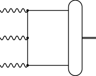
Figure 1: The lowest order o-Ps $\rightarrow 3\gamma$ decay graph. The factor on the right represents the initial spin-1 wave function.

where the sum is over the six permutations of the final state photons. The wave function factor is given by

$$\Psi=\sqrt{2M_{\rm Ps}}\begin{pmatrix}0&\vec{\sigma}\cdot\hat{\epsilon}/\sqrt{2}\\ 0&0\end{pmatrix}\phi_{0}\,,$$ (52)

which contains the spin-1 spin factor, a normalization factor, and the wave function at contact

$$\phi_{0}=\sqrt{\frac{m^{3}\alpha^{3}}{8\pi}}\,.$$ (53)

We write

$$\begin{pmatrix}0&\vec{\sigma}\cdot\hat{\epsilon}\\ 0&0\end{pmatrix}=\frac{1}{4}(\gamma N+1)\gamma\epsilon(\gamma N-1)$$ (54)

for the positronium spin factor where $N=P/(2W)$. The lowest order decay amplitude (see Fig. 1) becomes

$$M_{\rm{LO}}={\frac{-i\pi\alpha^{3}}{4}}\sum_{S_{3}}{\frac{1}{x_{1}x_{3}}}{\rm tr}\bigl{[}\gamma\epsilon^{*}_{3}(-\gamma R_{3}+1)\gamma\epsilon^{*}_{2}(\gamma R_{1}+1)\gamma\epsilon^{*}_{1}(\gamma N+1)\gamma\epsilon(\gamma N-1)\bigr{]}$$ (55)

where $R_{i}=N-K_{i}$, $K_{i}=k_{i}/W$ and $W\approx m$. The lowest order decay tensor has the corresponding form

$$M^{\mu_{1}\mu_{2}\mu_{3}\alpha}_{\rm LO}={\frac{-i\pi\alpha^{3}}{4}}\sum_{S_{3}}{\frac{1}{x_{1}x_{3}}}{\rm tr}\bigl{[}\gamma^{\mu_{3}}(-\gamma R_{3}+1)\gamma^{\mu_{2}}(\gamma R_{1}+1)\gamma^{\mu_{1}}(\gamma N+1)\gamma^{\alpha}(\gamma N-1)\bigr{]}\quad.$$ (56)

We replace $N$ by $(K_{1}+K_{2}+K_{3})/2$ and expand this out, and identify the $A_{i}$ functions by use of Eq. (14). The lowest order functions are

$$A^{\rm LO}_{1}(x_{1},x_{2},x_{3}) = 0\quad,$$ (57)

$$A^{\rm LO}_{2}(x_{1},x_{2},x_{3}) = 16i\pi m^{2}\alpha^{3}{\frac{\bar{x}_{1}\bar{x}_{2}\bar{x}_{3}}{x_{1}x_{2}x_{3}}}\quad,$$ (58)

$$A^{\rm LO}_{3}(x_{1},x_{2},x_{3}) = 0\quad,$$ (59)

where $x_{i}=\bar{s}_{jk}/M_{\rm Ps}^{2}$ and $\bar{x}_{i}=1-x_{i}=s_{jk}/M_{\rm Ps}^{2}$. Clearly, $A^{\rm{LO}}_{2}$ is a factor in each helicity amplitude. One has

$$M^{\rm{LO}}_{++--} = {\frac{-x_{3}}{\bar{x}_{1}\bar{x}_{2}}}\frac{A^{\rm{LO}}_{2}}{m^{2}}\quad,$$ (60)

$$M^{\rm{LO}}_{+-++} = M^{\rm{LO}}_{+---}={\frac{-1}{x_{3}\bar{x}_{3}}}\frac{A^{\rm{LO}}_{2}}{m^{2}}\quad,$$ (61)

$$M^{\rm{LO}}_{+-+-} = {\frac{-\bar{x}_{2}}{\bar{x}_{1}x_{3}}}\frac{A^{\rm{LO}}_{2}}{m^{2}}\quad,$$ (62)

$$M^{\rm{LO}}_{+--+} = {\frac{-\bar{x}_{1}}{\bar{x}_{2}x_{3}}}\frac{A^{\rm{LO}}_{2}}{m^{2}}\quad,$$ (63)

$$M^{\rm{LO}}_{+-+0} = {\frac{\bar{x}_{2}}{x_{3}}}\sqrt{\frac{2}{\bar{x}_{1}\bar{x}_{2}\bar{x}_{3}}}\frac{A^{\rm{LO}}_{2}}{m^{2}}\quad,$$ (64)

$$M^{\rm{LO}}_{+--0} = {\frac{\bar{x}_{1}}{x_{3}}}\sqrt{\frac{2}{\bar{x}_{1}\bar{x}_{2}\bar{x}_{3}}}\frac{A^{\rm{LO}}_{2}}{m^{2}}\quad,$$ (65)

with all other $M^{\rm{LO}}_{+\lambda_{2}\lambda_{3}\lambda}$ amplitudes equal to zero. One finds that

$$\overline{|M_{\rm{LO}}|^{2}}={\frac{512}{3}}\pi^{2}\alpha^{6}\Bigl{\{}\Bigl{(}{\frac{\bar{x}_{1}}{x_{2}x_{3}}}\Bigr{)}^{2}+\Bigl{(}{\frac{\bar{x}_{2}}{x_{1}x_{3}}}\Bigr{)}^{2}+\Bigl{(}{\frac{\bar{x}_{3}}{x_{1}x_{2}}}\Bigr{)}^{2}\Bigr{\}}\quad.$$ (66)

The lowest order decay rate is the Ore and Powell result Ore49

$$\Gamma_{\rm{LO}} = {\frac{2}{9\pi}}m\alpha^{6}\int_{0}^{1}dx_{1}\int_{1-x_{1}}^{1}dx_{2}\Bigl{\{}\Bigl{(}{\frac{\bar{x}_{1}}{x_{2}x_{3}}}\Bigr{)}^{2}+\Bigl{(}{\frac{\bar{x}_{2}}{x_{1}x_{3}}}\Bigr{)}^{2}+\Bigl{(}{\frac{\bar{x}_{3}}{x_{1}x_{2}}}\Bigr{)}^{2}\Bigr{\}}$$ (67)

$$= {\frac{2}{9\pi}}(\pi^{2}-9)m\alpha^{6}\quad.$$ (68)

VI One-Loop Integrals

We used the method of Passarino and Veltman Passarino79 to evaluate the one-loop integrals. Since this approach is widely used, and lengthy to describe in detail, we will just list the one-loop integrals that are required but only work the scalar integrals out in detail. The Passarino-Veltman method will be illustrated in the case of the three-point functions.

The general definition of the one-loop form factors is through

$$\bigl{\{}X_{0},X_{\mu},X_{\mu\nu},\cdots\bigr{\}} = \mu^{2\epsilon}\int(dq)^{\prime\prime}_{n}\,\bigl{\{}1,q_{\mu},q_{\mu}q_{\nu},\cdots\bigr{\}}$$ (69)

$$\times \bigl{[}(-q^{2}+m_{1}^{2})(-(q+p_{1})^{2}+m_{2}^{2})(-(q+p_{1}+p_{2})^{2}+m_{3}^{2})\cdots\bigr{]}^{-1}\,.$$ (70)

Ultraviolet divergences are controlled through dimensional regularization with $n=4-2\epsilon$ the dimensionality of spacetime. We define $(dq)^{\prime\prime}_{n}=d^{n}q/(i\pi^{n/2})$. The quantity $\mu$ is a reference mass introduced with the regularization which we take to be equal to the electron mass $m$. Functional dependences on the masses and momenta are indicated by $X(m_{1},m_{2},m_{3},\cdots;p_{1},p_{2},\cdots)$.

The one-point function is trivially evaluated:

$$A(m_{1}) = m^{2\epsilon}\int(dq)^{\prime\prime}_{n}{\frac{1}{(-q^{2}+m_{1}^{2})}}$$ (71)

$$= -m_{1}^{2}\Gamma(\epsilon)+\bar{A}(m_{1})+O(\epsilon)$$ (72)

where

$$\bar{A}(m_{1})=-m_{1}^{2}\bigl{[}1-\ln(m_{1}^{2}/m^{2})\bigr{]}\quad.$$ (73)

The two-point functions are defined by

$$\bigl{\{}B_{0},B_{\mu},B_{\mu\nu}\bigr{\}}=m^{2\epsilon}\int(dq)^{\prime\prime}_{n}\,\bigl{\{}1,q_{\mu},q_{\mu}q_{\nu}\bigr{\}}\bigl{[}(-q^{2}+m_{1}^{2})(-(q+p)^{2}+m_{2}^{2})\bigr{]}^{-1}\quad.$$ (74)

The scalar function $B_{0}$ is

$$B_{0}(m_{1},m_{2};p) = m^{2\epsilon}\int dx{\frac{\Gamma(\epsilon)}{\Delta^{\epsilon}}}$$ (75)

$$= \Gamma(\epsilon)+\bar{B}_{0}(m_{1},m_{2};p)$$ (76)

where $\Delta=(1-x)m_{1}^{2}+xm_{2}^{2}-x(1-x)p^{2}$ and

$$\bar{B}_{0}(m_{1},m_{2};p)=-\int dx\ln\bigl{(}\Delta/m^{2}\bigr{)}\quad.$$ (77)

All parametric integrals will be taken between the limits $0$ and $1$. The cases of interest are

$$\bar{B}_{0}(0,m;p)=2+{\frac{1-\rho}{\rho}}\ln(1-\rho)$$ (78)

where $\rho=p^{2}/m^{2}$, and

$$\bar{B}_{0}(m,m;p)=2\Bigl{\{}1-\sqrt{\frac{4-\rho}{\rho}}\arctan{\sqrt{\frac{\rho}{4-\rho}}}\Bigr{\}}\quad,$$ (79)

valid for $0\leq\rho\leq 4$.

The three-point functions are defined by

$$\bigl{\{}C_{0},C_{\mu},C_{\mu\nu},C_{\mu\nu\alpha}\bigr{\}} = m^{2\epsilon}\int(dq)^{\prime\prime}_{n}\,\bigl{\{}1,q_{\mu},q_{\mu}q_{\nu},q_{\mu}q_{\nu}q_{\alpha}\bigr{\}}$$ (80)

$$\times \bigl{[}(-q^{2}+m_{1}^{2})(-(q+p_{1})^{2}+m_{2}^{2})(-(q+p_{1}+p_{2})^{2}+m_{3}^{2})\bigr{]}^{-1}\,.$$ (81)

The general forms for $C_{\mu}$, $C_{\mu\nu}$, and $C_{\mu\nu\alpha}$ are

$$C_{\mu} = p_{1\mu}C_{11}+p_{2\mu}C_{12}\quad,$$ (82a)

$$C_{\mu\nu} = p_{1\mu}p_{1\nu}C_{21}+p_{2\mu}p_{2\nu}C_{22}+\{p_{1}p_{2}\}_{\mu\nu}C_{23}+g_{\mu\nu}C_{24}\quad,$$ (82b)

$$C_{\mu\nu\alpha} = p_{1\mu}p_{1\nu}p_{1\alpha}C_{31}+p_{2\mu}p_{2\nu}p_{2\alpha}C_{32}+\{p_{1}p_{1}p_{2}\}_{\mu\nu\alpha}C_{33}$$ (82d)

$$\quad+\{p_{1}p_{2}p_{2}\}_{\mu\nu\alpha}C_{34}+\{p_{1}g\}_{\mu\nu\alpha}C_{35}+\{p_{2}g\}_{\mu\nu\alpha}C_{36}\quad,$$

where

$$\{pk\}_{\mu\nu} = p_{\mu}k_{\nu}+k_{\mu}p_{\nu}\quad,$$ (83)

$$\{ppk\}_{\mu\nu\alpha} = p_{\mu}p_{\nu}k_{\alpha}+p_{\mu}k_{\nu}p_{\alpha}+k_{\mu}p_{\nu}p_{\alpha}\quad,$$ (84)

$$\{pg\}_{\mu\nu\alpha} = p_{\mu}g_{\nu\alpha}+p_{\nu}g_{\mu\alpha}+p_{\alpha}g_{\mu\nu}\quad.$$ (85)

The only divergent terms here are $C_{24}$, $C_{35}$, and $C_{36}$.

We illustrate the Passarino-Veltman procedure by describing the evaluation of $C_{11}$ and $C_{12}$ in terms of $C_{0}$ and the $B$ functions. We start by multiplying Eq. (82a) by $p_{1}^{\mu}$ and $p_{2}^{\mu}$:

$$p_{1}^{2}C_{11}+p_{12}C_{12} = \langle q\cdot p_{1}\rangle_{C}\equiv R_{1}\quad,$$ (86a)

$$p_{12}C_{11}+p_{2}^{2}C_{12} = \langle q\cdot p_{2}\rangle_{C}\equiv R_{2}\quad,$$ (86b)

where $p_{ij}=p_{i}\cdot p_{j}$ and $\langle\,\rangle_{C}$ is the integral operator on the RHS of Eq. (80) (so that for example $C_{0}=\langle 1\rangle_{C}$). We write Eqs. (86) as

$$X\begin{pmatrix}C_{11}\\ C_{12}\end{pmatrix}=\begin{pmatrix}R_{1}\\ R_{2}\end{pmatrix}\quad,\quad X=\begin{pmatrix}p_{1}^{2}&p_{12}\\ p_{12}&p_{2}^{2}\end{pmatrix}$$ (87)

with the solution

$$\begin{pmatrix}C_{11}\\ C_{12}\end{pmatrix}=X^{-1}\begin{pmatrix}R_{1}\\ R_{2}\end{pmatrix}\quad.$$ (88)

We find $R_{1}$ and $R_{2}$ by noting that

$$q\cdot p_{1} = {\frac{-1}{2}}\bigl{\{}-(-q^{2}+m_{1}^{2})+(-(q+p_{1})^{2}+m_{2}^{2})+f_{1}\bigr{\}}\quad,$$ (89a)

$$q\cdot p_{2} = {\frac{-1}{2}}\bigl{\{}-(-(q+p_{1})^{2}+m_{2}^{2})+(-(q+p_{1}+p_{2})^{2}+m_{3}^{2})+f_{2}\bigr{\}}\quad,$$ (89b)

where

$$f_{1} = m_{1}^{2}-m_{2}^{2}+p_{1}^{2}\quad,$$ (90a)

$$f_{2} = m_{2}^{2}-m_{3}^{2}+(p_{1}+p_{2})^{2}-p_{1}^{2}\quad.$$ (90b)

Then we see that

$$R_{1} = \langle q\cdot p_{1}\rangle_{C}={\frac{-1}{2}}\bigl{\{}-B_{0}(m_{2},m_{3};p_{2})+B_{0}(m_{1},m_{3};p_{1}+p_{2})$$ (91b)

$$\quad+f_{1}C_{0}(m_{1},m_{2},m_{3};p_{1},p_{2})\bigr{\}}\quad,$$

$$R_{2} = \langle q\cdot p_{2}\rangle_{C}={\frac{-1}{2}}\bigl{\{}-B_{0}(m_{1},m_{3};p_{1}+p_{2})+B_{0}(m_{1},m_{2};p_{1})$$ (91d)

$$\quad+f_{2}C_{0}(m_{1},m_{2},m_{3};p_{1},p_{2})\bigr{\}}\quad.$$

Since the $B$ functions are already known, only the scalar $C_{0}$ function remains to be computed. Similarly, the $C_{2i}$ functions can be evaluated in terms of the $C_{1i}$’s and $B$’s, etc. At each level in the ladder, only the scalar functions are new.

The general three-point scalar integral is

$$C_{0}(m_{1},m_{2},m_{3};p_{1},p_{2}) = \int(dq)^{\prime\prime}\bigl{[}(-q^{2}+m_{1}^{2})(-(q+p_{1})^{2}+m_{2}^{2})$$ (93)

$$\quad\quad\times(-(q+p_{1}+p_{2})^{2}+m_{3}^{2})\bigr{]}^{-1}$$

$$= \int dzdx{\frac{z}{\Delta}}\quad,$$ (94)

where the limit $n\rightarrow 4$ has been taken since $C_{0}$ is ultraviolet finite, and $(dq)^{\prime\prime}\equiv(dq)^{\prime\prime}_{4}=d^{4}q/(i\pi^{2})$. For $\Delta$ one finds

$$\Delta=(1-z)m_{1}^{2}+z(1-x)m_{2}^{2}+zxm_{3}^{2}-z(1-z)p_{1}^{2}-xz(1-z)2p_{12}-xz(1-xz)p_{2}^{2}\quad.$$ (95)

The cases of interest here are

$$C_{0}(0,m,m;p_{1},p_{2})={\frac{1}{2p_{12}}}\Bigl{\{}{\rm Li}_{2}\Bigl{(}{\frac{p_{1}^{2}+2p_{12}}{m^{2}}}\Bigr{)}-{\rm Li}_{2}\Bigl{(}{\frac{p_{1}^{2}}{m^{2}}}\Bigr{)}\Bigr{\}}$$ (96)

which holds when $p_{2}^{2}=0$;

$$C_{0}(0,m,m;p_{1},p_{2})={\frac{1}{2m^{2}\alpha}}\Bigl{\{}{\rm Li}_{2}(1-2\alpha)+2\zeta(2)-2\Bigl{(}\arctan\sqrt{\frac{1-\alpha}{\alpha}}\,\,\Bigr{)}^{2}\Bigr{\}}\quad,$$ (97)

which holds when $p_{1}^{2}=m^{2}$ and $(2p_{1}+p_{2})^{2}=0$ and where $\alpha=2+p_{12}/m^{2}$; and

$$C_{0}(m,m,m;p_{1},p_{2})={\frac{-1}{2p_{12}}}\Bigl{\{}{\rm L}\Bigl{(}{\frac{(p_{1}+p_{2})^{2}}{m^{2}}}\Bigr{)}-{\rm L}\Bigl{(}{\frac{p_{1}^{2}}{m^{2}}}\Bigr{)}\Bigr{\}}$$ (98)

where $p_{2}^{2}=0$ and

$${\rm L}(s)=\int dz{\frac{\ln(1-z(1-z)s)}{(1-z)}}=-2\Bigl{(}\arctan\sqrt{\frac{s}{4-s}}\,\Bigr{)}^{2}\quad.$$ (99)

The dilogarithm function ${\rm Li}_{2}(x)$ is discussed in detail by Lewin. Lewin81

The four-point functions are defined by

$$\bigl{\{}D_{0},D_{\mu},D_{\mu\nu},D_{\mu\nu\alpha},D_{\mu\nu\alpha\beta}\bigr{\}} = \int(dq)^{\prime\prime}\,\bigl{\{}1,q_{\mu},q_{\mu}q_{\nu},q_{\mu}q_{\nu}q_{\alpha},q_{\mu}q_{\nu}q_{\alpha}q_{\beta}\bigr{\}}\quad\quad\hbox{}$$ (100)

$$\times \bigl{[}(-q^{2}+m_{1}^{2})(-(q+p_{1})^{2}+m_{2}^{2})(-(q+p_{1}+p_{2})^{2}+m_{3}^{2})$$ (101)

$$\times (-(q+p_{1}+p_{2}+p_{3})^{2}+m_{4}^{2})\bigr{]}^{-1}\quad.$$ (102)

We have dispensed with the regularization here since all of the $D$ functions needed for our calculation are ultraviolet finite. While general expressions for $D_{0}$ exist, we need only a few special cases. In particular, we find that

$$D_{0}(0,m,m,m;mN,-k_{1},-k_{2})={\frac{8}{\sqrt{s_{12}\bar{s}_{12}s_{23}\bar{s}_{23}}}}\Bigl{\{}{\rm Li}_{2}\Bigl{(}{\frac{x_{+}}{\sqrt{D}}},\theta\Bigr{)}-{\rm Li}_{2}\Bigl{(}{\frac{-x_{-}}{\sqrt{D}}},\theta\Bigr{)}\Bigr{\}}\quad,$$ (103)

where

$$D = {\frac{m^{2}\bar{s}_{12}}{s_{12}\bar{s}_{23}}}\quad,$$ (104a)

$$x_{\pm} = {\frac{1}{2}}\Bigl{(}1\pm\sqrt{\frac{s_{23}\bar{s}_{12}}{s_{12}\bar{s}_{23}}}\,\,\Bigr{)}\quad,$$ (104b)

$$\tan\theta = \sqrt{\frac{\bar{s}_{23}}{s_{23}}}\quad,$$ (104c)

and ${\rm Li}_{2}(r,\theta)$ is the dilogarithm of complex argument. Lewin81 By some transformations among the momentum vectors, one can show that

$$D_{0}(0,m,m,m;mN-k_{1},-k_{2},-k_{3})=D_{0}(0,m,m,m;mN,-k_{3},-k_{2})\quad.$$ (105)

Finally, we also have

$$D_{0}(m,m,m,m;-k_{1},-k_{2},-k_{3}) = {\frac{-4}{\sqrt{s_{12}\bar{s}_{12}s_{23}\bar{s}_{23}}}}\Bigl{\{}{\rm Li}_{2}\Bigl{(}{\frac{y_{+}}{\sqrt{D_{1}}}},\theta_{1}\Bigr{)}-{\rm Li}_{2}\Bigl{(}{\frac{-y_{-}}{\sqrt{D_{1}}}},\theta_{1}\Bigr{)}$$ (108)

$$+{\rm Li}_{2}\Bigl{(}{\frac{y_{+}}{\sqrt{D_{3}}}},\theta_{3}\Bigr{)}-{\rm Li}_{2}\Bigl{(}{\frac{-y_{-}}{\sqrt{D_{3}}}},\theta_{3}\Bigr{)}$$

$$-{\rm Li}_{2}\Bigl{(}{\frac{y_{+}}{\sqrt{D_{0}}}},0\Bigr{)}+{\rm Li}_{2}\Bigl{(}{\frac{-y_{-}}{\sqrt{D_{0}}}},0\Bigr{)}\Bigr{\}}\quad,$$

where

$$D_{0} = {\frac{\bar{s}_{12}\bar{s}_{23}}{4s_{12}s_{23}}}\quad,$$ (109a)

$$D_{1} = {\frac{m^{2}\bar{s}_{23}}{s_{12}s_{23}}}\quad,$$ (109b)

$$D_{3} = {\frac{m^{2}\bar{s}_{12}}{s_{12}s_{23}}}\quad,$$ (109c)

$$y_{\pm} = {\frac{1}{2}}\bigl{(}1\pm 2\sqrt{D_{0}}\,\bigr{)}\quad,$$ (109d)

$$\theta_{1} = \arctan\sqrt{\frac{s_{12}}{\bar{s}_{12}}}\quad,$$ (109e)

$$\theta_{3} = \arctan\sqrt{\frac{s_{23}}{\bar{s}_{23}}}\quad.$$ (109f)

All of these integrals were done directly by way of Feynman parameters.

The five-point functions are required for the ladder diagram. The five-point functions are very difficult to evaluate in general. We require only a special case, where $m_{1}=0$, $m_{2}=m_{3}=m_{4}=m_{5}=m$, $p_{1}=mN$, $p_{2}=-k_{1}$, $p_{3}=-k_{2}$, $p_{4}=-k_{3}$. One feature of this special case is that there is a binding singularity: the scalar five-point function diverges, so we will have to base our implementation of the Passarino-Veltman formalism on the integral of the vector $q_{\mu}$, which is finite, instead of on the divergent scalar integral. Also, we have not yet evaluated the three- and four-point functions with the necessary momenta. We give the three-, four-, and five-point functions with the special case mass and momenta values the names $E$, $F$, and $G$:

$$\langle f\rangle_{E} = m^{2\epsilon}\int(dq)^{\prime\prime}_{n}\,f\bigl{[}(-q^{2})(-(q+p_{1})^{2}+m^{2})(-(q-p_{1})^{2}+m^{2})\bigr{]}^{-1}\quad,$$ (110a)

$$\langle f\rangle_{F(p_{2})} = m^{2\epsilon}\int(dq)^{\prime\prime}_{n}\,f\bigl{[}(-q^{2})(-(q+p_{1})^{2}+m^{2})(-(q-p_{1})^{2}+m^{2})$$ (110c)

$$\quad\times(-(q+p_{1}+p_{2})^{2}+m^{2})\bigr{]}^{-1}\quad,$$

$$\langle f\rangle_{G(p_{2},p_{3})} = m^{2\epsilon}\int(dq)^{\prime\prime}_{n}\,f\bigr{[}(-q^{2})(-(q+p_{1})^{2}+m^{2})(-(q-p_{1})^{2}+m^{2})$$ (110e)

$$\quad\times(-(q+p_{1}+p_{2})^{2}+m^{2})(-(q+p_{1}+p_{2}+p_{3})^{2}+m^{2})\bigr{]}^{-1}\quad,$$

where $p_{1}=p=mN$. The first two of these are special cases of the three- and four-point functions. Because of the binding singularity, $E_{0}=\langle 1\rangle_{E}$, $F_{0}=\langle 1\rangle_{F}$, and $G_{0}=\langle 1\rangle_{G}$ all diverge. We start our analysis with the vector integrals $E_{\mu}=\langle q_{\mu}\rangle_{E}$, $F_{\mu}=\langle q_{\mu}\rangle_{F}$, and $G_{\mu}=\langle q_{\mu}\rangle_{G}$.

The three-point special case vector integral has the general form

$$E_{\mu}=\langle q_{\mu}\rangle_{E}=p_{\mu}E_{1}\quad.$$ (111)

It is not hard to show (by use of symmetric integration) that $E_{1}=0$, so that

$$E_{\mu}=0\quad.$$ (112)

The four-point special case vector integral has the general form

$$F_{\mu}(p_{2})=\langle q_{\mu}\rangle_{F}=p_{1\mu}F_{11}(p_{2})+p_{2\mu}F_{12}(p_{2})\quad.$$ (113)

The necessary vector integrals for $p_{2}=-k_{1}$ are

$$F_{11}(-k_{1}) = {\frac{-1}{4x_{1}^{2}}}\Bigl{\{}{\rm Li}_{2}(1-2x_{1})-2x_{1}\ln(2x_{1})-2\theta^{2}-4\sqrt{x_{1}\bar{x}_{1}}\theta+2\zeta(2)\Bigr{\}}\quad,$$ (114a)

$$F_{12}(-k_{1}) = {\frac{1}{x_{1}}}F_{11}(-k_{1})+{\frac{1}{8x_{1}^{2}}}\bigl{[}2{\rm Li}_{2}(1-2x_{1})+\zeta(2)-2\theta^{2}\bigr{]}\quad$$ (114b)

where

$$\theta=\arctan{\sqrt{\frac{\bar{x}_{1}}{x_{1}}}}\quad.$$ (115)

When $p_{2}=-k_{1}-k_{2}$ one finds

$$F_{\mu}(-k_{1}-k_{2})=-F_{\mu}(-k_{3})\quad,$$ (116)

which implies that

$$F_{11}(-k_{1}-k_{2}) = -F_{11}(-k_{3})+2F_{12}(-k_{3})\quad,$$ (117)

$$F_{12}(-k_{2}-k_{2}) = F_{12}(-k_{3})\quad.$$ (118)

The five-point special case vector integral has the general form

$$G_{\mu}(-k_{1},-k_{2})=\langle q_{\mu}\rangle_{G}=p_{\mu}G_{11}+k_{1\mu}G_{12}+k_{3\mu}G_{13}\quad.$$ (119)

The $G_{1i}$ functions are given by

$$G_{11}(x_{1},x_{3}) = \frac{1}{8\bar{x}_{1}}\bigl{[}I_{0}(x_{1},x_{3})+I_{1}(x_{1},x_{3})\bigr{]}-\frac{1}{8\bar{x}_{3}}\bigl{[}I_{0}(x_{3},x_{1})+I_{1}(x_{3},x_{1})\bigr{]}\quad,$$ (120a)

$$G_{12}(x_{1},x_{3}) = \frac{1}{16x_{1}\bar{x}_{1}}\bigl{[}(1-2x_{1})I_{0}(x_{1},x_{3})-I_{1}(x_{1},x_{3})\bigr{]}$$ (120c)

$$\quad+\frac{1}{16x_{1}\bar{x}_{3}}\bigl{[}I_{0}(x_{3},x_{1})+I_{1}(x_{3},x_{1})\bigr{]}\quad,$$

$$G_{13}(x_{1},x_{3}) = \frac{-1}{16\bar{x}_{1}x_{3}}\bigl{[}I_{0}(x_{1},x_{3})+I_{1}(x_{1},x_{3})\bigr{]}$$ (120e)

$$\quad-\frac{1}{16x_{3}\bar{x}_{3}}\bigl{[}(1-2x_{3})I_{0}(x_{3},x_{1})-I_{1}(x_{3},x_{1})\bigr{]}\quad,$$

where

$$I_{0}(x_{1},x_{3}) = \frac{1}{\sqrt{x_{1}\bar{x}_{1}x_{3}\bar{x}_{3}}}\bigl{[}{\rm Li}_{2}(r_{+},\theta)-{\rm Li}_{2}(r_{-},\theta)\bigr{]}\quad,$$ (121a)

$$I_{1}(x_{1},x_{3}) = \frac{1}{(x_{1}-x_{3})}\ln\Bigl{(}\frac{x_{1}}{x_{3}}\Bigr{)}-\frac{2}{\sqrt{x_{3}\bar{x}_{3}}}\arctan\Bigl{(}\sqrt{\frac{\bar{x}_{3}}{x_{3}}}\Bigr{)}\quad,$$ (121b)

with $r_{\pm}=\sqrt{\bar{x}_{1}}\pm\sqrt{x_{1}\bar{x}_{3}/x_{3}}$ and $\theta=\arctan\sqrt{x_{1}/\bar{x}_{1}}$.

VII Analysis of the one-loop decay diagrams

The decay amplitudes can be written as

$$A_{i}=A_{i}^{(0)}+A_{i}^{(1)}+A_{i}^{(2)}+\cdots$$ (122)

for $i=1,2,3$, where the superscript indicates the power of $\alpha$ above that of the lowest order amplitudes $A_{i}^{(0)}=A_{i}^{LO}$. (Terms of order $A_{i}^{(2)}$ and higher also contain factors of $\ln(1/\alpha)$.) The expressions for the squares $|M_{\lambda_{1},\lambda_{2},\lambda_{3};m}|^{2}$ contain parts of the form

$$A_{i}^{*}A_{j}=A_{i}^{(0)*}A_{j}^{(0)}+\bigl{[}A_{i}^{(0)*}A_{j}^{(1)}+A_{i}^{(1)*}A_{j}^{(0)}\bigr{]}+A_{i}^{(1)*}A_{j}^{(1)}+\bigl{[}A_{i}^{(0)*}A_{j}^{(2)}+A_{i}^{(2)*}A_{j}^{(0)}\bigr{]}+\cdots$$ (123)

for various combinations of $i$ and $j$. The $A_{i}^{(0)*}A_{j}^{(0)}$ terms give the lowest-order differential decay distribution. The $A_{i}^{(0)*}A_{j}^{(1)}+A_{i}^{(1)*}A_{j}^{(0)}$ terms give the order-$\alpha$ correction, and the $A_{i}^{(1)*}A_{j}^{(1)}$ and $A_{i}^{(0)*}A_{j}^{(2)}+A_{i}^{(2)*}A_{j}^{(0)}$ terms give the order-$\alpha^{2}$ corrections.

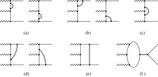
The graphs contributing to the order-$\alpha$ corrected decay amplitudes $A^{(1)}_{i}$ in the renormalized Feynman gauge are shown in Fig. 2. The infrared divergence induced by mass-shell renormalization is regulated by use of a photon mass $\lambda$. The self-energy (Fig. 2a) and vertex graphs (Figs. 2b, 2c) contain infrared divergences of the form $\ln\lambda M_{LO}$. The ladder graph Fig. 2e requires special care in its evaluation since it contains an infrared binding singularity. This divergence can be identified and subtracted out, as discussed in detail in Ref. Adkins02 . The result is that

$$M_{L}=\Bigl{\{}\frac{\pi}{\lambda}+\ln\lambda-1+O(\lambda)\Bigr{\}}\Bigl{(}\frac{\alpha}{\pi}\Bigr{)}M_{LO}+M_{LS}\quad.$$ (124)

The subtracted ladder graph is

$$M_{LS}=-i\alpha^{4}m^{2}\sum_{S_{3}}\int(d\ell)^{\prime\prime}\bigl{[}\ell^{2}(\ell^{2}-2\ell p)(\ell^{2}+2\ell p)Z(\ell)\bigr{]}^{-1}\Bigl{\{}\bigl{(}{\rm tr}(\ell)-{\rm tr}(0)\bigr{)}-{\frac{{\rm tr}(0)}{Z(0)}}\bigl{(}Z(\ell)-Z(0)\bigr{)}\Bigr{\}}\quad,$$ (125)

Figure 2: Graphs contributing to the o-Ps decay amplitudes through order-$\alpha$. They are the (a) self-energy, (b) outer vertex, (c) inner vertex, (d) double vertex, (e) ladder, and (f) annihilation contributions. The wave function factors are implicit in these graphs.

with $p=mN$,

$${\rm tr}(\ell) = {\frac{1}{4}}{\rm tr}\bigl{[}\gamma^{\mu}(\gamma(\ell-p)+m)\gamma\epsilon^{*}_{3}(\gamma(\ell-p+k_{3})+m)\gamma\epsilon^{*}_{2}(\gamma(\ell+p-k_{1})+m)$$ (127)

$$\times\gamma\epsilon^{*}_{1}(\gamma(\ell+p)+m)\gamma_{\mu}(\gamma N+1)\gamma\epsilon(\gamma N-1)\bigr{]}\quad,$$

and

$$Z(\ell)=((\ell-p+k_{3})^{2}-m^{2})((\ell+p-k_{1})^{2}-m^{2})\quad.$$ (128)

The subtraction in Eq.(125) takes away the $\ell$-independent part of ${\rm tr}(\ell)/Z(\ell)$, which would have had an infrared singularity. This binding singularity, regulated by the photon mass, is displayed in Eq. (124). The contributions of the order-$\alpha$ decay graphs were evaluated one by one and summed. The $1/\lambda$ binding singularity was removed according to the usual procedure of NRQED Caswell86 ; Adkins02 . The $\ln\lambda$ terms cancel between the self-energy, vertex, and ladder graphs. The remaining expressions are a finite sums of rational functions of the $x_{i}$ times logarithms, dilogarithms, and inverse tangent functions.

VIII Results and Conclusions

We use our analytic results for the order-$\alpha$ decay amplitudes $A^{(1)}_{i}$ to calculate the order-$\alpha$ correction to the o-Ps $\rightarrow 3\gamma$ decay rate and a part of the order-$\alpha^{2}$ correction. The individual amplitudes are quite lengthy and will not be displayed. A simplified form for the complete order-$\alpha$ decay rate contribution is given in the Appendix. The result for the order-$\alpha$ decay rate is integration_ref_1

$$\Gamma_{1}=-10.286606(10){\frac{\alpha}{\pi}}\Gamma_{LO}\quad.$$ (129)

This represents a 60-fold improvement in precision over the previous best result $-10.2866(6)$ Adkins92 done using a higher dimensional integration. The two-dimensional integral for the part of the order-$\alpha^{2}$ correction to the decay rate coming from the $A_{i}^{(1)*}A_{j}^{(1)}$ terms gives integration_ref_2

$$\Gamma_{2}({\rm square})=28.860(2)\Bigl{(}{\frac{\alpha}{\pi}}\Bigr{)}^{2}\Gamma_{LO}\quad.$$ (130)

The previous result for this contribution was $28.8(2)$. Burichenko93

In this work we obtained analytic expressions for the o-Ps$\rightarrow 3\gamma$ decay amplitudes. We used these expressions to obtain precise results for the one-loop and “square” decay rate contributions, which were incorporated into the full calculation of two-loop corrections to the o-Ps$\rightarrow 3\gamma$ decay rate. Adkins00 ; Adkins02 We also give an explicit form for the one-loop decay distribution (see the Appendix) which can be used to obtain the one-loop energy spectrum in a convenient form.

*

Appendix A The one-loop correction

In the appendix we present the integral for the one-loop correction to the decay rate in compact form. From this integral the one-loop phase-space distribution and energy spectrum can be obtained. We note that for very soft photons additional effects must be taken into account in order to obtain accurate results for the phase-space distribution and energy spectrum. Pestieau02 ; Manohar04 ; Voloshin04 ; Ruiz04

The one-loop correction to the decay rate is

$$\Gamma_{1}={\frac{m\alpha^{7}}{36\pi^{2}}}\int_{0}^{1}dx_{1}\int_{1-x_{1}}^{1}dx_{2}\,{\frac{1}{x_{1}x_{2}x_{3}}}\bigl{\{}F(x_{1},x_{3})+{\rm permutations}\bigr{\}}\quad,$$ (131)

where $x_{1}+x_{2}+x_{3}=2$ and the “permutations” are the six permutations of the variables $x_{1}$, $x_{2}$, $x_{3}$. The one-loop phase space distribution is just the integrand. The energy spectrum is found by integrating over $x_{2}$ but not $x_{1}=E_{1}/m$. (The corresponding lowest-order expression is given in Eq. (68).) The function $F(x_{1},x_{3})$ is given by

$$F(x_{1},x_{3})=g_{0}(x_{1},x_{3})+\sum_{i=1}^{5}g_{i}(x_{1},x_{3})h_{i}(x_{1})+\sum_{i=6}^{7}g_{i}(x_{1},x_{3})h_{i}(x_{1},x_{3})\quad.$$ (132)

The $h$ functions are given by

$$h_{1}(x_{1}) = \ln(2x_{1})\quad,$$ (133a)

$$h_{2}(x_{1}) = \sqrt{\frac{x_{1}}{\bar{x}_{1}}}\theta_{1}\quad,$$ (133b)

$$h_{3}(x_{1}) = {\frac{1}{2x_{1}}}\Bigl{\{}\zeta(2)-{\rm Li}_{2}(1-2x_{1})\Bigr{\}}\quad,$$ (133c)

$$h_{4}(x_{1}) = {\frac{1}{2x_{1}}}\Bigl{\{}\bigl{(}{\frac{\pi}{2}}\bigr{)}^{2}-\theta_{1}^{2}\Bigr{\}}\quad,$$ (133d)

$$h_{5}(x_{1}) = {\frac{1}{2\bar{x}_{1}}}\theta_{1}^{2}\quad,$$ (133e)

$$h_{6}(x_{1},x_{3}) = \frac{1}{\sqrt{x_{1}\bar{x}_{1}x_{3}\bar{x}_{3}}}\Bigl{\{}{\rm Li}_{2}(r_{A}^{+},\bar{\theta}_{1})-{\rm Li}_{2}(r_{A}^{-},\bar{\theta}_{1})\Bigr{\}}\quad,$$ (133f)

$$h_{7}(x_{1},x_{3}) = \frac{1}{\sqrt{x_{1}\bar{x}_{1}x_{3}\bar{x}_{3}}}\Bigl{\{}{\rm Li}_{2}(r_{B}^{+},\theta_{1})-{\rm Li}_{2}(r_{B}^{-},\theta_{1})$$ (133g)

$$\quad-\frac{1}{2}{\rm Li}_{2}(r_{C}^{+},0)+\frac{1}{2}{\rm Li}_{2}(r_{C}^{-},0)\Bigr{\}}\quad,$$

where $\bar{x}_{i}=1-x_{i}$ and

$$\theta_{1} = \arctan\bigl{(}\sqrt{\bar{x}_{1}/x_{1}}\,\,\bigr{)}\quad,$$ (134a)

$$\bar{\theta}_{1} = \arctan\bigl{(}\sqrt{x_{1}/\bar{x}_{1}}\,\,\bigr{)}\quad,$$ (134b)

$$r_{A}^{\pm} = \sqrt{\bar{x}_{1}}\Bigl{(}1\pm\sqrt{\frac{x_{1}\bar{x}_{3}}{\bar{x}_{1}x_{3}}}\,\Bigr{)}\quad,$$ (134c)

$$r_{B}^{\pm} = \sqrt{x_{1}}\Bigl{(}1\pm\sqrt{\frac{\bar{x}_{1}\bar{x}_{3}}{x_{1}x_{3}}}\,\Bigr{)}\quad,$$ (134d)

$$r_{C}^{\pm} = r_{B}^{\pm}/\sqrt{x_{1}}\quad.$$ (134e)

The $g$ functions are given in terms of $x^{mn}=x_{1}^{m}x_{3}^{n}$ and $\bar{x}_{2}=x_{1}+x_{3}-1$ as

$$g_{0}(x_{1},x_{3}) = {\frac{1}{9x_{1}\bar{x}_{1}(1-2x_{1})x_{3}\bar{x}_{3}(1-2x_{3})}}\Bigl{\{}-180+2196x^{10}-4968x^{20}$$ (135d)

$$+5292x^{30}-2664x^{40}+504x^{50}-5848x^{11}+22639x^{21}-20280x^{31}$$

$$+8405x^{41}-1240x^{51}-24x^{61}-17551x^{22}+22982x^{32}-5857x^{42}$$

$$+264x^{52}+48x^{62}-3776x^{33}-878x^{43}+400x^{53}+536x^{44}\Bigr{\}}\quad,$$

$$g_{1}(x_{1},x_{3}) = {\frac{4}{x_{1}^{2}(1-2x_{1})^{2}(x_{1}-x_{3})x_{3}}}\Bigl{\{}2x^{20}-13x^{30}+35x^{40}-36x^{50}+8x^{60}$$ (135h)

$$+4x^{70}+9x^{11}-59x^{21}+149x^{31}-210x^{41}+162x^{51}-51x^{61}+x^{71}$$

$$-4x^{02}+3x^{12}+55x^{22}-126x^{32}+104x^{42}-39x^{52}+x^{62}+8x^{03}$$

$$-26x^{13}+7x^{23}+22x^{33}+2x^{43}-2x^{53}-4x^{04}+14x^{14}-8x^{24}-8x^{34}\Bigr{\}}\quad,$$

$$g_{2}(x_{1},x_{3}) = {\frac{2}{3x_{1}^{3}\bar{x}_{1}x_{3}}}\Bigl{\{}-48x^{10}+180x^{20}-276x^{30}+228x^{40}-108x^{50}+24x^{60}$$ (135l)

$$+48x^{01}-48x^{11}-144x^{31}+244x^{41}-106x^{51}+2x^{61}+4x^{71}-96x^{02}$$

$$+156x^{12}-108x^{22}+168x^{32}-132x^{42}+7x^{52}+6x^{62}+48x^{03}-60x^{13}$$

$$-36x^{23}+42x^{33}+9x^{43}-6x^{53}+6x^{34}-4x^{44}\Bigr{\}}\quad,$$

$$g_{3}(x_{1},x_{3}) = {\frac{4}{x_{1}^{2}(x_{1}-x_{3})x_{3}}}\Bigl{\{}-2x^{20}-2x^{40}-4x^{60}+5x^{11}-6x^{21}+14x^{31}-4x^{41}$$ (135o)

$$+18x^{51}-x^{61}-4x^{02}-2x^{12}+4x^{22}-2x^{32}-26x^{42}-x^{52}+8x^{03}$$

$$-7x^{13}-2x^{23}+12x^{33}+2x^{43}-4x^{04}+4x^{14}\Bigr{\}}\quad,$$

$$g_{4}(x_{1},x_{3}) = {\frac{8}{x_{1}^{2}}}\Bigl{\{}-4+7x^{10}-7x^{20}+12x^{30}-10x^{40}+2x^{50}+8x^{01}-10x^{11}$$ (135q)

$$+3x^{21}-3x^{31}+2x^{41}-4x^{02}+3x^{12}+2x^{22}+x^{32}\Bigr{\}}\quad,$$

$$g_{5}(x_{1},x_{3}) = {\frac{2\bar{x}_{1}}{x_{1}}}\Bigl{\{}8-34x^{10}+29x^{20}-4x^{30}+6x^{11}+8x^{02}-4x^{12}\Bigr{\}}\quad,$$ (135r)

$$g_{6}(x_{1},x_{3}) = {\frac{1}{x_{1}\bar{x}_{2}x_{3}}}\Bigl{\{}16-76x^{10}+136x^{20}-124x^{30}+64x^{40}-16x^{50}-60x^{01}$$ (135v)

$$+272x^{11}-424x^{21}+294x^{31}-104x^{41}+22x^{51}+92x^{02}-392x^{12}$$

$$+484x^{22}-187x^{32}+13x^{42}+2x^{52}-76x^{03}+294x^{13}-259x^{23}+30x^{33}$$

$$+3x^{43}+36x^{04}-120x^{14}+61x^{24}+3x^{34}-8x^{05}+22x^{15}+2x^{25}\Bigr{\}}\quad,$$

$$g_{7}(x_{1},x_{3}) = {\frac{1}{\bar{x}_{2}}}\Bigl{\{}16-48x^{10}+46x^{20}-12x^{30}-2x^{40}-48x^{01}+60x^{11}+9x^{21}$$ (135x)

$$-31x^{31}+10x^{41}+46x^{02}+9x^{12}-42x^{22}+11x^{32}-12x^{03}-31x^{13}$$

$$+11x^{23}-2x^{04}+10x^{14}\Bigr{\}}\quad.$$

References

(1) S. G. Karshenboim, Int. J. Mod. Phys. A 19, 3879 (2004).
(2) W. Bernreuther and O. Nachtmann, Z. Phys. C 11, 235 (1981).
(3) R. Alcorta and J. A. Grifols, Ann. Phys. (N.Y.) 229, 109 (1994).
(4) J. Govaerts and M. Van Caillie, Phys. Lett. B 381, 451 (1996).
(5) A. Czarnecki and S. G. Karshenboim, hep-ph/9911410.
(6) P. A. Vetter, Int. J. Mod. Phys. A 19, 3865 (2004).
(7) S. N. Gninenko, N. V. Krasnikov, and A. Rubbia, Mod. Phys. Lett. A 17, 1713 (2002).
(8) A. Rubbia, Int. J. Mod. Phys. A 19, 3961 (2004).
(9) M. Deutsch, Phys. Rev. 83, 866 (1951).
(10) G. S. Adkins, R. N. Fell, and J. Sapirstein, Ann. Phys. (N.Y.) 295, 136 (2002).
(11) D. Sillou, Int. J. Mod. Phys. A 19, 3919 (2004).
(12) C. I. Westbrook, D. W. Gidley, R. S. Conti, and A. Rich, Phys. Rev. A 40, 5489 (1989).
(13) J. S. Nico, D. W. Gidley, A. Rich, and P. W. Zitzewitz, Phys. Rev. Lett. 65, 1344 (1990).
(14) W. E. Caswell, G. P. Lepage, and J. Sapirstein, Phys. Rev. Lett. 38, 488 (1977).
(15) W. E. Caswell and G. P. Lepage, Phys. Rev. A 20, 36 (1979).
(16) M. I. Dobroliubov, S. N. Gninenko, A. Yu. Ignatiev, and V. A. Matveev, Int. J. Mod. Phys. A 8, 2859 (1993).
(17) V. V. Dvoeglazov, R. N. Faustov, and Y. N. Tyukhtyaev, Mod. Phys. Lett. A 8, 3263 (1993).
(18) M. Skalsey, Materials Sci. Forum 255-257, 209 (1997).
(19) P. A. Vetter, Mod. Phys. Lett. A 19, 871 (2004).
(20) S. Asai, S. Orito, and N. Shinohara, Phys. Lett. B 357, 475 (1995).
(21) O. Jinnouchi, S. Asai, and T. Kobayashi, hep-ex/0011011.
(22) G. S. Adkins, R. N. Fell, and J. Sapirstein, Phys. Rev. Lett. 84, 5086 (2000).
(23) R. J. Hill and G. P. Lepage, Phys. Rev. D 62, 111301(R) (2000).
(24) B. A. Kniehl and A. A. Penin, Phys. Rev. Lett. 85, 1210 (2000); 85, 3065(E) (2000).
(25) K. Melnikov and A. Yelkhovsky, Phys. Rev. D 62, 116003 (2000).
(26) O. Jinnouchi, S. Asai, and T. Kobayashi, Phys. Lett. B 572, 117 (2003).
(27) R. S. Vallery, P. W. Zitzewitz, and D. W. Gidley, Phys. Rev. Lett. 90, 203402 (2003).
(28) P. Crivelli, Int. J. Mod. Phys. A 19, 3819 (2004).
(29) S. N. Gninenko, Int. J. Mod. Phys. A 19, 3939 (2004).
(30) G. S. Adkins, Phys. Rev. Lett. 76, 4903 (1996).
(31) E. W. N. Glover and A. G. Morgan, Z. Phys. C 60, 175 (1993).
(32) A. Ore and J. L. Powell, Phys. Rev. 75, 1696 (1949).
(33) G. Passarino and M. Veltman, Nucl. Phys. B 160, 151 (1979).
(34) The conventions and natural units [, ] of J. D. Bjorken and S. D. Drell, Relativistic Quantum Mechanics (McGraw-Hill, New York, 1964)] are used throughout. The symbol represents the electron mass.
(35) L. Lewin, Polylogarithms and Associated Functions (Elsevier North Holland, New York, 1981).
(36) W. E. Caswell and G. P. Lepage, Phys. Lett. 167B, 437 (1986).
(37) The adaptive Monte Carlo integration routine Vegas [G. P. Lepage, J. Comput. Phys. 27, 192 (1978)] was used for both and .
(38) G. S. Adkins, A. A. Salahuddin, and K. E. Schalm, Phys. Rev. A 45, 7774 (1992).
(39) Quadruple precision was required in order to retain numerical
significance in some parts of the integrand. The reported result
was obtained with approximately function calls.
(40) A. P. Burichenko, Yad. Fiz. 56, 123 (1993) [translated as Phys. At. Nucl. 56, 640 (1993)].
(41) J. Pestieau and C. Smith, Phys. Lett. B 524, 395 (2002).
(42) A. V. Manohar and P. Ruiz-Femenía, Phys. Rev. D 69, 053003 (2004).
(43) M. B. Voloshin, Mod. Phys. Lett. A 19, 181 (2004).