Pions emerging from an Arbitrarily Disoriented Chiral Condensate.

Relativistic heavy ion collisions either with fixed target or with head on collisions are providing results which suggest that the chiral phase transition does take place with temperatures crossing 170Mev. The comparatively large sizes of the heavy ions involved in the collisions along with their energy/nucleon, provides a large interaction region for the quarks and gluons. This region is where the Quark Gluon Plasma (QGP) forms. The picture we therefore have is that of a collision region where a QGP is formed in a highly non-equilibrium situation with chiral symmetry being restored. This plasma then expands and cools, causing the restored chiral symmetry to be broken once again. In a recent paper [1], we have given a quantum field theoretical model providing multiplicities of pions which would be observed if the QGP undergoes a rapid quench in its expansion or if the expansion is adiabatic. It was also shown how the rapid quench scenario, which is appropriate for the formation of the disoriented chiral condensate (DCC) has a enhancement in the multiplicities of the observed pions. Thus the enhancement signatures in the pion multiplicities are signals for the formation of the DCC also. In our analysis, we had assumed the expansion of the QGP to be isotropic for simplicity. However, recent results from RHIC suggest that there may be anisotropy built in from the nature of the collisions. Not all collisions will be head on with zero impact parameter. There will be instances where there will be non-zero impact parameter causing the impact region to be elliptical and the corresponding QGP to have an elliptical flow. From the nature of our quantum field theoretical model, borrowing from the studies of scalar fields on expanding universes, such as the Friedmann-Robertson-Walker universe, it is easy to extend the study to include anisotropy such as that caused by an elliptic flow. We shall report these results elsewhere, in a separate communication [2]. Here, we shall be examining another aspect of the restoration of chiral symmetry. The particular form of our model allows for many metastable states through which the DCC can form. In particular, we find that mixing between various erstwhile pion states in the collision region can produce different signals in the multiplicities of the final state pions.
We start with an $O(4)$ quartet of scalar fields in order that we can construct the dynamics of quenched pions in the formation of a disoriented chiral condensate. The background field is the classical disoriented vacuum and the Hamiltonian of the quantum fluctuations around the background field is derived from the $O(4)$ sigma model keeping one-loop quantum corrections (quadratic order in the fluctuations)[1]. The resulting dynamical Hamiltonian for the pion and sigma fields fields in terms of the neutral , charged pion and sigma creation and annihilation operators ($a,a^{{\dagger}},c,c^{{\dagger}},b$ $b^{{\dagger}}$, and $d,d^{{\dagger}}$) is[1]:

$$H = \int\frac{d^{3}\underline{k}}{(2\pi)^{3}}\frac{1}{2}\{\frac{\omega_{\pi}}{a^{3}}(a_{k}^{{\dagger}}a_{k}+a_{k}a^{{\dagger}}_{k})+\frac{\omega_{\pi}}{2a^{3}}(\frac{\Omega_{\pi}^{2}}{\omega_{\pi}^{2}}-1)(a_{k}^{{\dagger}}a_{k}+a_{k}a_{k}^{{\dagger}}+a_{-k}a_{k}+a_{-k}^{{\dagger}}a_{k}^{{\dagger}})$$

$$+ \frac{\omega_{\Sigma}}{a^{3}}(d_{k}^{{\dagger}}d_{k}+d_{k}d^{{\dagger}}_{k})+\frac{\omega_{\Sigma}}{2a^{3}}(\frac{\Omega_{\Sigma}^{2}}{\omega_{\Sigma}^{2}}-1)(d_{k}^{{\dagger}}d_{k}+d_{k}d_{k}^{{\dagger}}+d_{-k}d_{k}+d_{-k}^{{\dagger}}d_{k}^{{\dagger}})\}$$

$$+ \frac{\omega_{\pi}}{a^{3}}(b_{k}^{{\dagger}}b_{k}+c_{k}c^{{\dagger}}_{k})+\frac{\omega_{\pi}}{2a^{3}}(\frac{\Omega_{\pi_{\pm}}^{2}}{\omega_{\pi}^{2}}-1)(b_{k}^{{\dagger}}b_{k}+c_{k}c_{k}^{{\dagger}}+b_{-k}c_{k}+c_{-k}^{{\dagger}}b_{k}^{{\dagger}})$$

$$+ \frac{\lambda a^{3}v^{2}cos^{2}(\rho)sin^{2}(\theta)}{4\omega_{\pi}}(b_{k}b_{-k}+b_{k}c^{{\dagger}}_{k}+c^{{\dagger}}_{k}b_{k}+c_{k}c_{-k}+c^{{\dagger}}_{k}c^{{\dagger}}_{-k}+c_{k}b^{{\dagger}}_{k}+b^{{\dagger}}_{k}c_{k}+b^{{\dagger}}_{k}b^{{\dagger}}_{-k}))$$

$$+ \frac{\lambda a^{3}v^{2}cos(\rho)sin(\rho)sin^{2}(\theta)}{2\omega_{\pi}}\left(b_{k}a_{-k}+b_{k}a^{{\dagger}}_{k}+c^{{\dagger}}_{k}a_{k}+c_{k}a_{-k}+c^{{\dagger}}_{k}a^{{\dagger}}_{-k}+c_{k}a^{{\dagger}}_{k}+b^{{\dagger}}_{k}a_{k}+b^{{\dagger}}_{k}a^{{\dagger}}_{-k}\right)$$

$$+ \frac{\lambda a^{3}v^{2}sin(\rho)sin(\theta)cos(\theta)}{\sqrt{\omega_{\pi}\omega_{\Sigma}}}\left(d_{k}a_{-k}+d_{k}a^{{\dagger}}_{k}+d^{{\dagger}}_{k}a_{k}+d^{{\dagger}}_{k}a^{{\dagger}}_{-k}\right)$$

$$+ \frac{\lambda a^{3}v^{2}cos(\rho)sin(\theta)cos(\theta)}{\sqrt{\omega_{\pi}\omega_{\Sigma}}}\left(b_{k}d_{-k}+b_{k}d^{{\dagger}}_{k}+c^{{\dagger}}_{k}d_{k}+c_{k}d_{-k}+c^{{\dagger}}_{k}d^{{\dagger}}_{-k}+c_{k}d^{{\dagger}}_{k}+b^{{\dagger}}_{k}d_{k}+b^{{\dagger}}_{k}d^{{\dagger}}_{-k}\right)\}$$ (2)

where

$$\frac{\omega^{2}_{\pi}(k)}{a^{6}}\equiv\frac{\omega^{2}_{\pi_{0}}(k)}{a^{6}}=\frac{\omega^{2}_{\pi_{\pm}}(k)}{a^{6}}=(m_{\pi}^{2}+\frac{\underline{k}^{2}}{a^{2}}):\>\frac{\omega^{2}_{\Sigma}(k)}{a^{6}}=(m_{\Sigma}^{2}+\frac{\underline{k}^{2}}{a^{2}})$$ (3)

and

$$\frac{\Omega^{2}_{\pi_{0}}-\omega^{2}_{\pi_{0}}}{a^{6}} = \lambda[(<\Phi^{2}>-v^{2})+2v_{3}^{2}]$$

$$\frac{\Omega^{2}_{\pi{\pm}}-\omega^{2}_{\pi_{\pm}}}{a^{6}} = \lambda[(<\Phi^{2}>-v^{2})+2v_{+}v_{-}]$$

$$\frac{\Omega^{2}_{\Sigma}-\omega^{2}_{\Sigma}}{a^{6}} = \lambda[(<\Phi^{2}>-v^{2})+2\sigma^{2}]$$ (4)

The background field in the disoriented phase is given by :

$$\left(\begin{array}[]{c}v_{+}\\ v_{-}\\ v_{3}=v\\ \sigma\end{array}\right)\equiv<\Phi>,$$ (5)

In keeping with the disorientation of the vacuum on a three sphere we parametrize the background field through three angles:

$$<\Phi>=\left(\begin{array}[]{c}vCos(\rho)Sin(\theta)Sin(\alpha)\\ vCos(\rho)Sin(\theta)Cos(\alpha)\\ vSin(\rho)Sin(\theta)\\ vCos(\theta)\end{array}\right).$$ (6)

The dynamical evolution of a system governed by this Hamiltonian is considered from a non equilibrium state state of restored symmetry $<\Phi>=0$ at high temperatures to the equilibrium state of broken symmetry $<\Phi>=v$ due to the subsequent expansion and cooling of the QGP. The time evolution can be modeled through a time dependence of the parameter $<\Phi>(t)$, which depends on the way in which the system relaxes to equilibrium. In addition there is a time dependence of the expansion factor $a(t)$ which allows for the rate of the expansion of the plasma. The following scenarios are possible:
A. A sudden quench from a state of restored symmetry to a state of broken symmetry in a rapidly cooling expanding plasma, the configuration of the field lags behind the expansion of the plasma.If $\tau$ is the time the state spends in the symmetry restored phase, a quench can be modeled by assuming that for $0$ the vacuum expectation value $<\Phi^{2}>=0$ and for $t>\frac{\tau}{2}$ the vacuum relaxes to its value $<\Phi^{2}>=<v^{2}>$. In such a case the dynamical evolution of $<\Phi>$ could be modeled by $<\Phi>(t)=v\Theta[(t-\tau)]$ In addition in a realistic scenario the expansion coefficient $a(t)$ must also be a function of time and has been modeled appropriately in ref [1]. For a sudden quench scenario the Hamiltonian given in equation 1 diagonalizes to

$$H=\int\frac{d^{3}\underline{k}}{(2\pi)^{3}}\frac{1}{2a^{3}}\{\Omega_{\pi}(k,t)\{(A^{{\dagger}}_{k}A_{k}+\frac{1}{2})+(C^{{\dagger}}_{k}C_{k}+B^{{\dagger}}_{k}B_{k}+1)\}+\Omega_{\Sigma}(k,t)(D^{{\dagger}}_{k}D_{k}+\frac{1}{2})\}.$$ (7)

by a unitary matrix given by a squeezed transformation

$$U(r,t)=e^{\int\frac{d^{3}\underline{k}}{(2\pi)^{3}}r(k,t)\{(a^{{\dagger}}_{k}a^{{\dagger}}_{-k}-a_{k}a_{-k})+(d^{{\dagger}}_{k}d^{{\dagger}}_{-k}-d_{k}d_{-k})+(c_{k}b_{-k}+b_{k}c_{-k})-(c^{{\dagger}}_{k}b^{{\dagger}}_{-k}+b^{{\dagger}}_{k}c^{{\dagger}}_{-k})\}}$$ (8)

where $r_{k}$ is the squeezing parameter related to the physical variables $\Omega_{\pi}(k,t)$ and $\omega_{\pi}(k)$ through

$$Tanh(2r_{k})=\frac{(\frac{\Omega_{k}(t)}{\omega_{\pi}})^{2}-1}{(\frac{\Omega_{k}(t)}{\omega_{\pi}})^{2}+1}$$ (9)

The quench consists of a rapid change of frequency of the time dependent harmonic oscillator from $\Omega_{\pi}(k,t))$ to $\omega_{\pi}(k)$ though the time evolution of $<\Phi>(t)$ and $a(t)$. It can be shown that for a sudden frequency jump, such as that of a quench, there is substantial squeezing, resulting in an enhancement of low momentum modes signalling a DCC. The details of the evolution of the Hamiltonian of a system undergoing a sudden quench (enhanced squeezing) also show up in the difference in multiplicity distributions of the charged and neutral pions illustrated in Figure 1.

Figure 1: Shows the variation of $P_{n0}$ (solid line)and $P_{nc}$(dashed line) with $n$ for the quenched limit ($r_{0}=4$)

B. Another non-equilibrium situation that can arise is one where the system can go through a metastable disordered vacuum given by eqn[6] and then relax by quantum fluctuations to an equilibrium configuration. Here $\theta$ and $\rho$ measure the degree of disorientation of the condensate in isospin space ( for charge conservation $\alpha=\frac{\pi}{4}$) . The disorientation can be in the neutral sector $\rho=\frac{\pi}{2}$ in which case the angle $\theta$ mixes the neutral pion and sigma field resulting in oscillations and enhancement of neutral pions over the charged pions, we will call this case 1 . The disorientation can be in the charged sector $\theta=\frac{\pi}{2}$, where the angle $\rho$ mixes the charged pions and the neutral pions resulting in charged oscillations and enhancement of charged pions over the neutral pions we will call this case 2. As an illustration of these effects we examine case 1 briefly. All the details of case 1 and 2 will be given in an expanded later communication [2]. For case 1 the examination of the Hamiltonian ( obtained by putting $\rho=\frac{\pi}{2}$ ) shows a non-zero mixing term coming from the $\pi_{0}$-$\Sigma$ sector. The misalignment of the vacuum through an angle $\theta$ induces a mixing of the two fields. The mixed fields are

$$\left(\begin{array}[]{c}A_{\theta(k)}\\ D_{\theta(k)}\end{array}\right)=\left(\begin{array}[]{c}Cos(\theta)\;\;\;Sin(\theta)\\ -Sin(\theta)\;\;\;Cos(\theta)\end{array}\right)\left(\begin{array}[]{c}a_{k}\\ d_{k}\end{array}\right)$$ (10)

The diagonalization procedure for this case involves two squeezing transformations of the mixed fields

$$F_{k} = \mu A_{\theta(k)}+\nu A^{{\dagger}}_{\theta(-k)}$$

$$G_{k} = \rho D_{\theta(k)}+\sigma D^{{\dagger}}_{\theta(-k)}.$$ (11)

The diagonalized form is

$$H_{\pi/2}=\int\frac{d^{3}\underline{k}}{(2\pi)^{3}}\{\frac{\Omega_{\pi_{\pm}}}{a^{3}}(C^{{\dagger}}_{k}C_{k}+B^{{\dagger}}_{k}B_{k}+1)+\frac{\sqrt{\Omega_{\pi}\Omega_{\Sigma}}}{4a^{3}}\left((F^{{\dagger}}_{k}F_{k}+\frac{1}{2})+(G^{{\dagger}}_{k}G_{k}+\frac{1}{2})\right)\}$$ (12)

During time evolution again we have a time dependent frequency for the state of mixed neutral pions and sigma which changes from $\frac{\sqrt{\Omega_{\pi}(k,t)\Omega_{\Sigma}(k,t)}}{4a^{3}}$ to$\frac{\sqrt{\omega_{\pi}(k,t)\omega_{\Sigma}(k,t)}}{4a^{3}}$ this time through the time evolution of $\theta(t)$ from the disoriented value to 0 and $a(t)$. There is again an enhancement of neutral pions as a result of the DCC formation and furthermore a mixing in the neutral sector . In addition there are oscillations in the number of neutral pions as the disorientation $\theta$ changes with time shown in Figure 2.

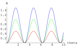
Figure 2: Shows the oscillations in the number of neutral pions as a function of the disorientation $\theta$ for the value of the squeezing parameters $"red=\nu=.5,green=\nu=1,blue=\nu=1.5$

A case of particular interest , in view of latest preliminary experimental results is case 2 i.e. $\theta=\frac{\pi}{2}$ because there is a mixing of charged and neutral fields due to the disorientation. This gives rise to interesting charge-neutral fluctuations which can be measured in a DCC detection experiment[3]. A full discussion of the detailed theory is given in [2].

To conclude we have modeled the evolution of the disoriented chiral condensate through both a sudden quench and with a transition through a metastable state with arbitrary disorientation and have shown that the total multiplicity distributions of charged and neutral pions functions are dramatic characteristic signals for the DCC and are related directly to the way in which the DCC forms. These are unambiguous, therefore they must be examined thoroughly in searches for the DCC [4]. We are encouraged by the first preliminary data of references [3] and [4], from the analysis of the WA98 experiment at the CERN SPS in which some events show an excess of photons (neutral pion excess) within the overlap region of charged and photon multiplicity detectors, the preliminary results given in ref [4] are shown in figure 3.

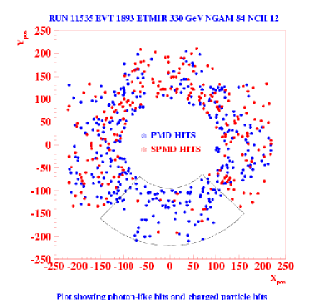
Figure 3: Shows the photon hits and charged particle hits in WA98 from ref. 4

In view of the results presented in this section, we hope that the future will bring more exotic events with charge excess and neutral and charged multiplicity oscillations.

References

• B. Bambah and C. Mukku, Phys. Rev. D. 70 (3) 0340001 (2004).
  B.A. Bambah and C.Mukku, Annals of Physics 314, 34,(2004)

• B. A. Bambah , C. Mukku and K.V.S Shiv Chaitanya Dynamics of the Dcc with Arbitrary Disorientation in Isospin Space( In preparation).

• T. Nayak ,Pramana 57 ,285,(2001).

• M.M. Aggarwal et al., e-print archive:nucl-ex/0012004.
  Madan M Aggarwal, Pramana 60, No.5, 987 , (2003)