Probing the Flavour Structure of Supersymmetry Breaking With Rare B–Processes – A Beyond Leading Order Analysis

Abstract:

In the framework of minimal supersymmetry with general flavour mixing in the squark sector we consider dominant beyond leading order (BLO) effects in the rare processes $\bar{B}\to X_{s}\gamma$, $\bar{B}_{s}\to\mu^{+}\mu^{-}$ and $\bar{B}_{s}-B_{s}$ mixing. We present analytic expressions for corrected vertices, which are applicable in general, and provide a recipe for the inclusion of the dominant and subdominant BLO effects in existing LO calculations. We also derive similar expressions in the mass insertion approximation. We investigate in more detail the focusing effect pointed out in our earlier work, which, at large $\tan\beta$ and $\mu>0$, leads to a reduced supersymmetric contribution to the above processes. We also find that, in some cases, flavour dependence, that accidentally cancels at leading order, can reappear at BLO. We further include electroweak corrections, which, while generally subdominant, in some cases may have a substantial effect. For example, their contribution to the charged Higgs vertex in $\bar{B}\to X_{s}\gamma$ can be of the order of 20% at BLO. They can also reduce the contribution of LL insertions to $\bar{B}_{s}\to\mu^{+}\mu^{-}$ and $\bar{B}_{s}-B_{s}$ mixing by up to 20%, even at the LO. We also analyse radiative generation of CKM elements and find the possibility that the CKM matrix elements $K_{ts}$ and $K_{cb}$ can be generated entirely by LR insertions. This work constitutes the first complete analysis of dominant BLO effects in the GFM scenario.

1 Introduction

Flavour physics, in both the leptonic and hadronic sectors, currently provides one of the best hopes of discovering, or at least constraining, new physics beyond the Standard Model (SM). In the hadronic sector in particular, decays mediated by flavour changing neutral currents (FCNC) play an important role as the Glashow–Iliopoulos–Maiani (GIM) mechanism [1] ensures that both SM and contributions due to beyond the SM (BSM) physics enter at the one–loop level. It is therefore possible that such contributions can be comparable to the SM ones, or even completely dominate the behaviour of the underlying process. Once one takes into account the increasingly accurate experimental data that is being gathered at both dedicated flavour physics experiments, as well as the B–physics programmes operating at collider experiments, useful constraints can often be placed on the parameters and mass scale of a given model of new physics. Conversely, for some processes, like $\bar{B}_{s}\to\mu^{+}\mu^{-}$, a measurement of a branching ratio at the Tevatron would immediately indicate a detection of BSM physics.

One of the most compelling extensions of the Standard Model is the Minimal Supersymmetric Standard Model (MSSM) [2]. The non–renormalization theorem of the underlying supersymmetric theory can explain the stability of scalar potentials in theories involving two different hierarchies. Additionally, the MSSM provides a viable cold dark matter candidate (namely the lightest supersymmetric particle), a natural scheme for gauge coupling unification, and is usually compatible with the precision electroweak data currently available.

Softly broken low–energy supersymmetry (SUSY), however, like most new physics schemes, allows for the possibility that contributions to FCNC and CP violating processes can exceed SM expectations by orders of magnitude (the flavour and CP problems). The source of the flavour problem in the MSSM is primarily due to the arbitrary nature soft supersymmetry breaking terms [2].

The most common approach to these problems is to assume that the underlying theory obeys the conditions imposed by minimal flavour violation (MFV) [3]. The definition of MFV, presented in [3], is that flavour violation is determined completely by the structure of the usual Yukawa couplings. In other words, the mixings among the down and up squarks are governed by the CKM matrix. In the MSSM this restricts the form the soft terms can take (see [3] for the exact expressions). One popular scheme, that respects MFV, is that the soft terms are universal at some high scale associated with supersymmetry (SUSY) breaking, like the grand unified scale or the Planck scale (a parameterisation used, for example, in the Constrained MSSM). However, this hypothesis is not renormalization group invariant. Flavour violating terms are induced, via running from the high scale $\Lambda$ to the characteristic mass scale of the squarks $\mu_{SUSY}$, that are proportional to $\log(\Lambda^{2}/\mu_{SUSY}^{2})/(4\pi^{2})$ [4]. It should be noted however, that, provided the theory satisfies MFV up to the scale $\Lambda$ (a rather strong assumption), all FCNC transitions remain proportional to the appropriate CKM matrix elements and the resulting low energy theory still satisfies the MFV hypothesis. However, once seeds of non–universality are introduced at the high scale it is possible that they can become amplified by running.

This provides motivation to generalise to a broader framework, namely general flavour mixing (GFM) in the sfermion sector. In general, the flavour structure of the soft terms is not protected by any symmetry and can be rather arbitrary. One simple example is that a degree of non–universality can be allowed in the squark soft terms (beyond that allowed by MFV). In this case additional effects are possible that are proportional, essentially, to the degree of splitting between the entries for each generation.

Deviations from MFV can easily appear in a variety of SUSY models. In theories with SUSY breaking mediated by supergravity, for example, it is possible to induce a wide range of flavour violating effects [5] once one proceeds beyond the simplest minimal SUGRA scheme [2]. Grand unified theories involving right handed neutrinos, like the minimal ${\rm SO}(10)$ models with a specific family structure, often lead to additional sources of flavour violation due to the interactions that exist, at the unification scale, between right–handed down squarks and neutrinos [6, 7, 8, 9, 10]. Experimental limits and results are therefore especially helpful when restricting the possible mixings between the various generations and constraining these models.

In this paper we shall concern ourselves chiefly with flavour violation between the second and third generations. FCNC processes involving such transitions have been studied in detail in the context of the SM and the short–distance contributions to a wide variety of processes have typically been calculated to NLO in the SM (the evaluation of long–distance effects is another matter). In the case of $\bar{B}\to X_{s}\gamma$ these efforts have resulted in a very good agreement between SM calculations and experimental results with relatively little room left for new physics. When placing constraints on a given model it is useful to have a calculation that is of a similar accuracy to the SM contribution. In the MSSM complete NLO calculations, however, are rather complicated as additional two–loop diagrams involving gluinos need to be evaluated. It is, however, possible to include the effects that are large once one proceeds beyond the LO (BLO). Such effects are typically classified as being proportional to either $\tan\beta$ or large logs. Such BLO analyses have been performed in MFV [11, 12, 3, 13, 14] and, more recently, in GFM [15, 16, 17]. In GFM, in particular, a focusing effect was found in [15] that gave rise to significant shifts in the allowed regions of parameter space compared to a LO analysis. (A similar effect appears also in the MFV scheme but is much weaker [15, 16].) Basically, in many cases of phenomenological interest (e.g., large $\tan\beta$ and $\mu>0$), SUSY contributions to $\bar{B}\to X_{s}\gamma$ are significantly reduced compared to the LO approximation. A similar effect was also found in the decay $\bar{B}_{s}\to\mu^{+}\mu^{-}$ and $\bar{B}_{s}-B_{s}$ mixing [17].

The aim of this paper is to present the first complete analysis of dominant BLO effects in general flavour mixing in the case of three processes. The first, $\bar{B}\to X_{s}\gamma$, has been discussed previously in [15, 16]. However, here we shall include the additional corrections that arise when one includes charginos and neutralinos in the resummation procedure discussed in [16]. In particular, we include contributions arising from higgsino exchange, that are proportional to the Yukawa couplings of the third generation, and the additional contributions to the charged Higgs vertex that were discussed in the context of MFV in [14].

The other two processes we shall consider are the decay $\bar{B}_{s}\to\mu^{+}\mu^{-}$ and $\bar{B}_{s}-B_{s}$ mixing. These processes have not been observed yet but have come under a lot of theoretical scrutiny lately due to the large contributions possible in the large $\tan\beta$ regime. In this paper we discuss the GFM contributions to both processes in detail, highlighting the effects that appear once one proceeds beyond the LO.

In all the three cases, we shall present the analytic expressions required to implement BLO corrections in the GFM scenario for possibly large deviations from the MFV scheme. However, since these general expressions are often rather complicated, we shall also derive expressions in the the mass insertion approximation (MIA), allowing the BLO effects to be shown explicitly. In both cases we will provide an explicit recipe for including the BLO effects into the existing LO expressions. Whilst we shall not include such effects in the forthcoming analysis, the formalism we shall present should, with relatively little modification, be applicable to the CP violating case.

The paper is organised as follows. In section 2 we summarise the formalism employed in this paper, giving complete expressions for all the corrected masses and vertices used in our calculation. In section 3 we present analytic expressions for these masses and vertices in the MIA. In section 4 we discuss the decay $\bar{B}\to X_{s}\gamma$ providing analytic expressions for the BLO corrections to supersymmetric and electroweak contributions in the MIA. In sections 5 and 6 we perform a similar analyses for the decay $\bar{B}_{s}\to\mu^{+}\mu^{-}$ and $\bar{B}_{s}-B_{s}$ mixing, respectively. Finally, in section 7 we present our numerical analysis.

2 Beyond Leading Order Effects and General Flavour Mixing

The influence of $\tan\beta$ enhanced effects on the down quark masses, the charged Higgs and neutral Higgs vertex are known to be large. It is therefore essential, especially when working in the large $\tan\beta$ regime, that such contributions are taken into account (and resummed if necessary).

In this section, we shall follow the method first developed in [15, 16] and generalise it to include the additional effects that appear once the contributions of chargino and neutralino loops are taken into account. It should be noted that the analysis below encompasses both MFV and the GFM scenario and can be easily extended to include, for example, CP violation or flavour violation in the leptonic sector.

2.1 The Framework

Once the supersymmetric particles have been integrated out, the effective Lagrangian describing the quark mass terms, at some scale $\mu<M_{SUSY}$, in the physical super–CKM basis (SCKM) is given by

$$-\mathcal{L}_{q}^{\rm mass}=\bar{d}_{R}\left(m_{d}^{(0)}+\delta m_{d}\right)d_{L}+\bar{u}_{R}\left(m_{u}^{(0)}+\delta m_{u}\right)u_{L}+h.c.,$$ (1)

where $d_{L,R}$ and $u_{L,R}$ denote the down and up components of the left and right quark fields, respectively. In the physical SCKM basis the quark mass matrices are, by definition, diagonal and it is possible to make the identifications

$$m_{d}= m_{d}^{(0)}+\delta m_{d}={\rm diag}\left(m_{d},m_{s},m_{b}\right),$$ (2)

$$m_{u}= m_{u}^{(0)}+\delta m_{u}={\rm diag}\left(m_{u},m_{c},m_{t}\right),$$ (3)

where $m_{d,s,b}$ and $m_{u,c,t}$ denote the physical masses of the down and up–type quarks respecitively. The bare mass matrix $m_{d}^{(0)}$ is related to the $3\times 3$ Yukawa couplings $Y_{d,u}^{\left(0\right)}$ derived from the superpotential in the usual manner,

$$m_{d,u}^{(0)}=v_{d,u}Y_{d,u}^{(0)}.$$ (4)

where $v_{d,u}=\langle H^{0}_{d,u}\rangle$. Finally, $\delta m_{d}$ and $\delta m_{u}$ denote the radiative corrections to the quark masses induced by integrating out the SUSY particles [18, 19, 20, 21]. The corrections have the form

$$\delta m_{d}=\Sigma^{d}_{m\,L}+\frac{1}{2}\Sigma_{v\,R}^{d}m_{d}^{(0)}+\frac{1}{2}m_{d}^{(0)}\Sigma_{v\,L}^{d}.$$ (5)

$\delta m_{u}$ is given by a similar formula after one performs the substitution $d\to u$. The $3\times 3$ hermitian matrices $\Sigma_{v\,L,R}^{d,u}$ and the $3\times 3$ complex matrices $\Sigma_{m\,L}^{d,u}$ denote the contributions arising from wavefunction and mass corrections due to two point diagrams involving gluinos, charginos, neutralinos and squarks. (Full expressions will be given later in the text.)

Before discussing how the radiative corrections $\delta m_{d}$ are calculated, it will be useful to consider the transformation from the interaction basis to the physical SCKM basis. In the interaction basis, the MSSM superpotential is

$$W_{F}=-\mu\hat{H}_{d}\hat{H}_{u}+Y_{l}^{(0)o}\hat{H}_{d}\hat{L}^{o}\hat{E}^{o}+Y_{d}^{(0)o}\hat{H}_{d}\hat{Q}^{o}\hat{D}^{o}-Y_{u}^{(0)o}\hat{H}_{u}\hat{Q}^{o}\hat{U}^{o},$$ (6)

$\hat{Q}^{o}$ and $\hat{L}^{o}$ are the quark and lepton ${\rm SU}\left(2\right)$ doublet superfields, $\hat{D}^{o}$, $\hat{U}^{o}$ and $\hat{E}^{o}$ denote the singlet superfields and $\hat{H}_{u}$ and $\hat{H}_{d}$ are the two Higgs doublets that appear in the MSSM (for more details see, for example, [2]), while $Y_{l,d,u}^{o}$ are the appropriate $3\times 3$ Yukawa mass matrices in that basis.

The soft SUSY breaking terms are also usually introduced in the interaction basis. The Lagrangian for the bilinear soft SUSY breaking terms is given by

$$-\mathcal{L}_{\widetilde{q}\,{\rm soft}}^{o\,{\rm mass}}= +\tilde{d}_{L}^{o{\dagger}}m_{Q}^{2}\tilde{d}_{L}^{o}+\tilde{d}_{R}^{o{\dagger}}m_{D}^{2}\tilde{d}_{R}^{o}+\left[\tilde{d}_{L}^{o{\dagger}}\left(v_{d}A_{d}^{\ast}\right)\tilde{d}_{R}^{o}+h.c.\right]$$

$$+\tilde{u}_{L}^{o{\dagger}}m_{Q}^{2}\tilde{u}_{L}^{o}+\tilde{u}_{R}^{o{\dagger}}m_{U}^{2}\tilde{u}_{R}^{o}+\left[\tilde{u}_{L}^{o{\dagger}}\left(v_{u}A_{u}^{\ast}\right)\tilde{u}_{R}^{o}+h.c.\right],$$ (7)

where $m_{Q}^{2}$, $m_{D}^{2}$ and $m_{U}^{2}$ are, in general, arbitrary $3\times 3$ hermitian matrices. The trilinear terms $A_{d}$ and $A_{u}$, on the other hand, are arbitrary $3\times 3$ complex matrices. We have not assumed that the trilinear soft terms are proportional to the appropriate Yukawa coupling. (We discuss an alternative parameterisation, that can be used in the GFM scenario, in appendix B.)

Transforming the quark fields from the interaction basis to the physical SCKM basis involves performing unitary transformations on both the left and right handed fields such that

$$d_{R} =V_{d_{R}}d_{R}^{o}, d_{L} =V_{d_{L}}d_{L}^{o},$$ (8)

$$u_{R} =V_{u_{R}}d_{R}^{o}, u_{L} =V_{u_{L}}d_{L}^{o}.$$ (9)

The bare mass matrix is then related to the Yukawa couplings defined in the interaction basis via the relation

$$m_{d}^{(0)}= V_{d_{R}}v_{d}Y_{d}^{(0)o}V_{d_{L}}^{\dagger}, m_{u}^{(0)}= V_{u_{R}}v_{u}Y_{u}^{(0)o}V_{u_{L}}^{\dagger},$$ (10)

$m_{d}^{(0)}$ and $m_{u}^{(0)}$ appear in all quantities derived from the superpotential (6) not subject to the corrections (5), such as the couplings of supersymmetric particles. The CKM matrix $K$ is related to the transformations (8)–(9) in the usual manner

$$K=V_{u_{L}}V_{d_{L}}^{{\dagger}}.$$ (11)

As the radiative corrections $\delta m_{d,u}$ are calculated in the SCKM basis, it is necessary to consider how the transformations (8)–(9), when performed on the squark fields, affect the relevant mass matrices. After transforming to the physical SCKM basis, the soft terms become

$$m_{d,LL}^{2}= V_{D_{L}}m_{Q}^{2}V_{D_{L}}^{{\dagger}}, m_{d,RR}^{2}= V_{D_{R}}m_{D}^{2}V_{D_{R}}^{{\dagger}}, m_{d,LR}^{2}= V_{D_{L}}\left(v_{d}A_{d}^{\ast}\right)V_{D_{R}}^{{\dagger}},$$

$$m_{u,LL}^{2}= V_{U_{L}}m_{Q}^{2}V_{U_{L}}^{{\dagger}}, m_{u,RR}^{2}= V_{U_{R}}m_{U}^{2}V_{U_{R}}^{{\dagger}}, m_{u,LR}^{2}= V_{U_{L}}\left(v_{u}A_{u}^{\ast}\right)V_{U_{R}}^{{\dagger}}.$$ (12)

The $6\times 6$ down squark mass matrix $\mathcal{M}_{\tilde{d}}^{2}$ may then be written in the following manner

$$\mathcal{M}_{\tilde{d}}^{2}=\left(\begin{array}[]{ll}m_{d,LL}^{2}+F_{d,LL}+D_{d,LL}{}{}&m_{d,LR}^{2}+F_{d,LR}\\ \left(m_{d,LR}^{2}+F_{d,LR}\right)^{\dagger}&m_{d,RR}^{2}+F_{d,RR}+D_{d,RR}\end{array}\right).$$ (15)

(The up squark mass matrix may be similarly defined by substituting $d$ with $u$.) The $F$–terms that appear in (15) are given by

$$F_{d,LL} =m_{d}^{(0)}{}^{\dagger}m_{d}^{(0)}, F_{d,RR} =m_{d}^{(0)}m_{d}^{(0)}{}^{\dagger}, F_{d,LR} =-\mu\tan\beta m_{d}^{(0)}{}^{\dagger},$$ (16)

and the flavour diagonal $D$–terms are

$$D_{d,LL} =m_{Z}\cos 2\beta\left(T_{3d}-Q_{d}\sin^{2}\theta_{W}\right){\mathchoice{\rm 1\mskip-4.0mul}{\rm 1\mskip-4.0mul}{\rm 1\mskip-4.5mul}{\rm 1\mskip-5.0mul}}_{3}, D_{d,RR}=m_{Z}\cos 2\beta Q_{d}\sin^{2}\theta_{W}{\mathchoice{\rm 1\mskip-4.0mul}{\rm 1\mskip-4.0mul}{\rm 1\mskip-4.5mul}{\rm 1\mskip-5.0mul}}_{3}.$$ (17)

It should be noted that, in the physical SCKM basis, the $F$–terms are, in general, not necessarily flavour diagonal as they are derived from the superpotential and are therefore functions of the bare mass matrix $m_{d}^{(0)}$.

To obtain the physical squark masses $m_{\widetilde{d}_{I}}$ it is necessary to perform an additional unitary transformation on the squark fields such that

$$\Gamma_{d}\mathcal{M}_{\tilde{d}}^{2}\Gamma_{d}^{{\dagger}}={\rm diag}\left(m_{\tilde{d}_{1}},\dots,m_{\tilde{d}_{6}}\right).$$ (18)

It is conventional to decompose the original $6\times 6$ unitary matrix $\Gamma_{d}$ into two $6\times 3$ submatrices $\Gamma_{d\,L}$ and $\Gamma_{d\,R}$:

$$\left(\Gamma_{d}\right)_{Ii}= \left(\Gamma_{d\,L}\right)_{Ii}, \left(\Gamma_{d}\right)_{Ii+3}= \left(\Gamma_{d\,R}\right)_{Ii}.$$ (19)

where $I=1,\dots,6$ and $i=1,2,3$.

Departures from the MFV scenario are often parameterised in terms of the dimensionless quantities

$$\left(\delta_{LL}^{d}\right)_{ij}= \frac{\left(m_{d,LL}^{2}\right)_{ij}}{\sqrt{\left(m_{d,LL}^{2}\right)_{ii}\left(m^{2}_{d,LL}\right)_{jj}}}, \left(\delta_{LR}^{d}\right)_{ij}= \frac{\left(m_{d,LR}^{2}\right)_{ij}}{\sqrt{\left(m_{d,LL}^{2}\right)_{ii}\left(m^{2}_{d,RR}\right)_{jj}}},$$ (20)

$$\left(\delta_{RL}^{d}\right)_{ij}= \frac{\left(m_{d,RL}^{2}\right)_{ij}}{\sqrt{\left(m_{d,RR}^{2}\right)_{ii}\left(m^{2}_{d,LL}\right)_{jj}}}, \left(\delta_{RR}^{d}\right)_{ij}= \frac{\left(m_{d,RR}^{2}\right)_{ij}}{\sqrt{\left(m_{d,RR}^{2}\right)_{ii}\left(m^{2}_{d,RR}\right)_{jj}}}.$$ (21)

The soft terms $m_{d,XY}^{2}$ ($X,Y=L,R$) are given in (12) and $i,j=1,2,3$. Similar definitions apply for the up quarks. It should be noted that, since $m^{2}_{u,LL}$ and $m^{2}_{d,LL}$ are related to one another by ${\rm SU}(2)$ invariance, we have the relation

$$\delta_{LL}^{d}=K^{{\dagger}}\delta_{LL}^{u}K$$ (22)

Let us briefly comment on the basis dependence of these definitions of $\delta^{d}_{XY}$. Physical quantities such as cross–sections and branching ratios are naturally independent of the basis in which one defines the soft terms. The basis in which one defines the insertions $\delta^{d}_{XY}$, however, is essentially a matter of convenience. As discussed above, we work in the physical SCKM basis throughout this analysis and as such the definition (20)–(21) is essentially the easiest to implement numerically. Other definitions of $\delta_{XY}^{d}$ have been used in the literature before, for example, one might define $\delta_{XY}^{d}$ in the uncorrected (bare) SCKM basis where the Yukawa matrices derived from the superpotential are diagonal (we shall define this basis more formally in subsection 3.4). Transforming between different bases involves performing additional unitary transformations on the soft terms (12) and, unless large non–universalities exist, the differences between the transformed and the original $\delta_{XY}^{d}$ are typically rather small. Below we will derive many expressions in the MIA where one usually assumes that the diagonal entries of the soft terms are universal. In light of the above we expect them to be applicable to alternative definitions of $\delta_{XY}^{d}$. During our numerical analysis we employ a similar definition for the SUSY soft terms to ensure that our formalism remains applicable to as wide a variety of models as possible.

After defining our framework, let us now move on to the effects that these corrections have on the electroweak and supersymmetric vertices.

2.2 Corrections to Electroweak Vertices

Integrating out the supersymmetric particles, coupled with the effect of transforming between the interaction and the physical SCKM bases, can affect the form of the electroweak (i.e. the Higgs and gauge boson) vertices present in the resulting effective theory.

After transforming to the physical SCKM basis, the W boson vertex has the following form

$$\mathcal{L}_{W}=\bar{u}_{L}\gamma^{\mu}C_{L}^{W}d_{L}W^{+}_{\mu}+\bar{u}_{R}\gamma^{\mu}C_{R}^{W}d_{R}W^{+}_{\mu}+h.c.$$ (23)

The $3\times 3$ coupling matrices $C_{L}^{W}$ and $C_{R}^{W}$, are given by

$$C_{L}^{W} =-\frac{g_{2}}{\sqrt{2}}\left(K+\frac{1}{2}\Sigma_{v\,L}^{u}K+\frac{1}{2}K\Sigma_{v\,L}^{d}\right)+\Delta C_{L}^{W}=-\frac{g_{2}}{\sqrt{2}}K^{\rm eff},$$ (24)

$$C_{R}^{W} =\Delta C_{R}^{W}.$$ (25)

We employ the notation $\Delta C_{L,R}^{X}$ to denote the vertex corrections that arise from three point diagrams when one integrates out the SUSY particles. Identifying the left handed coupling of the $W$ boson with the physical CKM matrix $K^{\rm eff}$, that is measured from experiment, we have the relation

$$K^{\rm eff}=K+\frac{1}{2}\Sigma_{v\,L}^{u}K+\frac{1}{2}K\Sigma_{v\,L}^{d}-\frac{\sqrt{2}}{g_{2}}\Delta C_{L}^{W}.$$ (26)

The uncorrected CKM matrix $K$ is defined in (11) and appears in all vertices not subject to the corrections (26).

Now consider the coupling of the $Z$ boson with down quarks

$$\mathcal{L}_{Z^{0}}=\bar{d}_{L}\gamma^{\mu}C_{L}^{Z}d_{L}Z^{0}_{\mu}+\bar{d}_{R}\gamma^{\mu}C_{R}^{Z}d_{R}Z^{0}_{\mu}.$$ (27)

The $3\times 3$ coupling matrices $C_{L}^{Z}$ and $C_{R}^{Z}$ are given by

$$C_{L}^{Z} =\frac{g_{2}}{2\cos\theta_{W}}\left(1-\frac{2}{3}\sin^{2}\theta_{W}\right)\left(1+\Sigma_{v\,L}^{d}\right)+\Delta C_{L}^{Z},$$ (28)

$$C_{R}^{Z} =-\frac{g_{2}}{2\cos\theta_{W}}\frac{2}{3}\sin^{2}\theta_{W}\left(1+\Sigma_{v\,R}^{d}\right)+\Delta C_{R}^{Z}.$$ (29)

The radiative corrections to $C_{L}^{Z}$ and $C_{R}^{Z}$ can induce off–diagonal elements to the coupling that lead to additional sources of FCNC.

Turning to the Higgs sector, the inclusion of radiative corrections is especially important. As the coupling between the Higgs sector and squarks features a dependence on the soft SUSY breaking terms (rather than only gauge interactions), the corrected vertices that arise when one integrates out the coloured SUSY particles can display a non–decoupling property. Large corrections to the vertices are therefore feasible for even  TeV scale sparticle masses.

Once one has integrated out the SUSY particles, the charged Higgs interaction becomes

$$\mathcal{L}_{S^{+}}=\bar{u}_{R}C^{S^{+}}_{L}d_{L}S^{+}+\bar{u}_{L}C^{S^{+}}_{R}d_{R}S^{+}+h.c.,$$ (30)

where $S^{+}=H^{+},G^{+}$ and the $3\times 3$ matrices coupling $C^{S^{+}}_{L,R}$ are given by

$$C^{S^{+}}_{L} =\frac{g_{2}}{\sqrt{2}m_{W}\sin\beta}y_{(1)}^{S^{+}}\left(m_{u}K-\Sigma^{u}_{m\,L}K-\frac{1}{2}m_{u}^{(0)}\Sigma^{u}_{v\,L}K+\frac{1}{2}m_{u}^{(0)}K\Sigma^{d}_{v\,L}\right)+\Delta C_{L}^{S^{+}},$$ (31)

$$C^{S^{+}}_{R} =\frac{g_{2}}{\sqrt{2}m_{W}\cos\beta}y_{(2)}^{S^{+}}\left(Km_{d}-K\Sigma^{d{\dagger}}_{m\,L}-\frac{1}{2}K\Sigma^{d}_{v\,L}m_{d}^{(0)}{}^{{\dagger}}+\frac{1}{2}\Sigma^{u}_{v\,L}Km_{d}^{(0)}{}^{{\dagger}}\right)+\Delta C_{R}^{S^{+}},$$ (32)

where $y_{(1)}^{S^{+}}=\cos\beta,\sin\beta$ and $y_{(2)}^{S^{+}}=\sin\beta,-\cos\beta$.

The neutral Higgs and Goldstone boson interact with the down quarks in the following way

$$\mathcal{L}_{S^{0}}=\bar{d}_{R}C_{L}^{S^{0}}d_{L}S^{0}+\bar{d}_{L}C_{R}^{S^{0}}d_{R}S^{0},$$ (33)

where $S^{0}=H^{0},h^{0},A^{0},G^{0}$ and the effective vertices $C_{R}^{S^{0}}$ and $C_{R}^{S^{0}}$ may be written in terms of the $3\times 3$ matrices

$$C_{L}^{S^{0}} =-\frac{g_{2}}{2m_{W}\cos\beta}x_{(1)}^{S^{0}}\left(m_{d}-\Sigma_{m\,L}^{d}\right)+\Delta C_{L}^{S^{0}},$$

$$C_{R}^{S^{0}} =-\frac{g_{2}}{2m_{W}\cos\beta}x_{(1)}^{S^{0}\ast}\left(m_{d}-\Sigma_{m\,L}^{d{\dagger}}\right)+\Delta C_{R}^{S^{0}}$$ (34)

and $x_{(1)}^{S^{0}}=\cos\alpha,-\sin\alpha,i\sin\beta,-i\cos\beta$.

In the limit where the physical SCKM basis is identical to the bare SCKM basis (i.e. where $m_{d}=m_{d}^{(0)}$), (34) is identical to the diagrammatic result derived in the on–shell formalism used in [22, 23].

2.3 Corrections to Supersymmetric Vertices

As the corrections to the electroweak vertices are calculated in the physical SCKM basis, it is necessary to discuss how the supersymmetric interactions are altered once transformed into this basis. Ignoring the effects of wavefunction renormalizations, that are not enhanced by $\tan\beta$, the changes introduced by transforming to the physical SCKM basis typically amount to the introduction of $m_{d}^{(0)}$ and $K$ into the various vertices. For instance, after these replacements have been performed, the chargino vertex becomes

$$\mathcal{L}_{\chi^{\pm}}= \;\sum_{a,i,J}\tilde{u}_{J}^{\dagger}\left(\bar{\chi}^{-}\right)_{a}\left[\left(C_{d\,L}\right)_{aJi}P_{L}+\left(C_{d\,R}\right)_{aJi}P_{R}\right]\left(d\right)_{i},$$ (35)

where $a=1,2$, $i=1,2,3$, and $J=1,\dots,6$ and the couplings $C_{d\,L}$ and $C_{d\,R}$ may be written in terms of the matrices

$$\left(C_{d\,L}\right)_{aJi}= -g_{2}V_{a1}^{\ast}\left(\Gamma_{u\,L}K\right)_{Ji}+\frac{g_{2}}{\sqrt{2}m_{W}\sin\beta}V_{a2}^{\ast}\left(\Gamma_{u\,R}m_{u}^{(0)}K\right)_{Ji},$$ (36)

$$\left(C_{d\,R}\right)_{aJi}= \frac{g_{2}}{\sqrt{2}m_{W}\cos\beta}U_{a2}^{\ast}\left(\Gamma_{u\,L}Km_{d}^{(0)}{}^{\dagger}\right)_{Ji},$$ (37)

where $K$ is defined in terms of the physical CKM matrix by $K^{\rm eff}$ in (26) and the bare masses are given by (3) and its analogue for the up quarks. The matrices $U$ and $V$ diagonalise the chargino mass matrix $\mathcal{M}_{\chi^{\pm}}$ such that

$$U\mathcal{M}_{\chi^{\pm}}V^{{\dagger}}={\rm diag}\left(m_{\chi_{1}^{\pm}},m_{\chi_{2}^{\pm}}\right).$$

The appearance of the bare quark mass matrix $m_{d}^{(0)}$ in these vertices can lead to large effects in both MFV and GFM models. A full list of vertices relevant to our calculation appear in Appendix C.

2.4 Numerical Aspects

Let us now discuss how the method discussed above should be implemented numerically. As we will be investigating values of up to $\mathcal{O}(1)$ for the flavour violating parameters $\delta_{XY}^{d}$ ($X,Y=L,R$) (20)–(21), it is important to devise a method such that the effects discussed in section 2 are taken into account, whilst also retaining the numerical accuracy associated with working in the squark mass basis. Such an iterative method was proposed in [16] and it will be useful for our purposes to briefly summarise it here.

Once the unitary transformations (18) have been performed on the squark fields the gluino contribution to $\delta m_{d}$ becomes [16]

$$\delta m_{d}=\frac{\alpha_{s}}{2\pi}\;C_{2}\left(3\right)\sum_{I=1}^{6}\left(\Gamma_{d\,R}^{\ast}\right)_{Ii}\left(\Gamma_{d\,L}\right)_{Ij}m_{\widetilde{g}}\,B_{0}\left(m_{\widetilde{g}}^{2},m_{\widetilde{d}_{I}}^{2}\right).$$

The Passarino–Veltman function $B_{0}$ can be found in appendix A.5. Using this relation it is possible to calculate the bare mass matrix using (3). It should be noted, however, that $\delta m_{d}$ contains a dependence on $m_{d}^{(0)}$ as it appears in the squark mass matrix through the $F$–terms (16). It is therefore necessary to employ an iterative procedure such that $m_{d}^{(0)}$ and the mixing matrices $\Gamma_{dL,R}$ are determined to the desired level of accuracy. The inclusion of the effects induced by chargino and neutralino contributions introduces a dependence on $m_{u}^{(0)}$ and the uncorrected CKM matrix $K$ in the formula for $\delta m_{d}$. One must therefore expand and generalise the iterative procedure presented in [16] such that these effects are included as well.

In the first step of the procedure, $m_{d}^{(0)}$, $m_{u}^{(0)}$ and $K$ are set equal to the input parameters $m_{d}$, $m_{u}$ and $K^{\rm eff}$, respectively, and $\delta m_{d,u}$ is set equal to zero. In the second step, the squark mass matrices and the supersymmetric couplings are then calculated with these input values, allowing the evaluation of the radiative corrections $\Sigma^{d}$, $\Sigma^{u}$ and $\Delta C_{L}^{W}$ using the formulae presented in appendix D. In the third step, $\delta m_{d,u}$, the bare mass matrices and $K$ are determined using (3) and (26). The resulting values are then used as the new input parameters in step two. The second and third steps are then repeated until convergence occurs. The iterative procedure converges rather rapidly and after $n$ iterations amounts to including the first $n$ terms that arise in a Taylor expansion in $\tan\beta$. For an example of the procedure applied to MFV, see [16]. With the final forms of the supersymmetric couplings, uncorrected CKM matrix and bare mass matrices determined, the corrections to the $Z$ boson, charged Higgs and neutral Higgs vertices may be calculated using the formulae presented in section 2.2 and appendix D. We should emphasise here that we work in the squark mass basis throughout and therefore include all the effects that can occur at higher orders in the MIA as well as the BLO effects described in the previous subsections. In addition, we include the effects induced by additional electroweak contributions, light quark effects and ${\rm SU}(2)_{L}\times{\rm U}(1)_{Y}$ breaking.

3 The Mass Insertion Approximation

Expressions for $m_{d}^{(0)}$ and the corrected vertices are well known in MFV models [25, 11, 14] and it will be useful for our purposes to extend these results to the GFM scenario. The flavour dependence of analytic expressions is often rather obscure when flavour violation is communicated via the matrices (19). To express the underlying dependence on the off–diagonal elements of the soft breaking terms it is therefore useful to work in the mass insertion approximation (MIA). According to this approximation the off–diagonal elements of $\mathcal{M}_{\tilde{d}}^{2}$ are treated as perturbations and enter expressions through mixed propagators proportional to the relevant element (or insertion). These insertions are parameterised in terms of the dimensionless quantities defined in (20)–(21). Equivalently, one may expand the matrices (19) about the diagonal. When performing actual numerical calculations it is more advantageous to diagonalise the squark mass matrices (15) using numerical routines to ensure that higher order terms in the MIA are included, this is what we shall do in our numerical analysis presented in section 7.

Before proceeding with our analytic expressions for the bare mass matrix and the various effective vertices, let us first outline the approximations we shall use throughout this section. As we are chiefly concerned in exhibiting the dominant behaviour displayed by the corrections to the bare mass matrix and effective vertices, in this section we shall work in the approximation of vanishing electroweak couplings and typically ignore ${\rm SU}(2)_{L}\times{\rm U}(1)_{Y}$ breaking effects. We therefore mainly concern ourselves with the effects induced by gluino exchange, and those that arise from higgsino exchange that are proportional to the Yukawa couplings of the third generation. Let us emphasise, however, that during our numerical analysis we include all the effects that arise from non–zero electroweak couplings, ${\rm SU}(2)_{L}\times{\rm U}(1)_{Y}$ breaking effects and the effects of the Yukawa couplings of the first two generations. Concerning the accuracy that we work to within the MIA, we typically include terms up to second order in the MIA (unless specified otherwise). We therefore do not include the effects of multiple diagonal LR insertions that are proportional to $m^{2}_{d,LR}-\mu m_{d}^{(0)}\tan\beta$. It is possible to resum the effects induced by these insertions via the method outlined in [23]. In this method however, some BLO effects are then encoded into the factors of $\cos\theta_{\widetilde{b}}$ and $\sin\theta_{\widetilde{b}}$ that appear in the MFV squark mixing matrices. Since the ultimate aim of this section is to present analytic expressions that represent all of the BLO corrections that appear in the framework presented in section 2, we shall only consider the effects of at most one flavour diagonal LR insertion. Converting our expressions to take into account such effects however should be relatively easy. Finally, to allow for easy comparison between our results and those that already exist in the literature, we have assumed that the trilinear up–type soft terms are proportional to the appropriate Yukawa coupling (i.e. $m^{2}_{u,LR}=m_{u}A_{u}$, where $A_{u}={\rm diag}(A_{u},A_{c},A_{t})$), although we still do not assume a similar relation for the down–squark sector, (it is easy to convert back by making the substitution $A_{t}\to\left(m^{2}_{u,LR}\right)_{33}/m_{t}$ in the various expressions that follow).

3.1 The Bare Mass Matrix in the MIA

We shall first consider the corrections induced by CKM and GFM effects on the bare mass matrix $m_{d}^{(0)}$. Loop corrections to the bare mass matrix in the MFV scenario were derived in [19, 25, 11]. They were subsequently generalised to GFM in [21, 15, 16].

The bare mass matrix may be determined by evaluating the self energy corrections that appear (5). The dominant contributions to $\Sigma^{d}_{m\,L}$ arise from self–energy diagrams involving gluino and chargino exchange, which are depicted in Fig. 1.

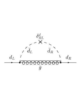
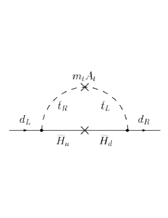
Figure 1: The dominant gluino and higgsino diagrams that contribute to $\Sigma^{d}_{m\,L}$.

On the other hand, the corrections to $\Sigma^{d}_{v\,L,R}$ are rather small when compared to those that arise from $\Sigma^{d}_{m\,L}$ as they are not enhanced by $\tan\beta$, nor do they feature a chirality flip on the gluino line. Coupled with the suppression factors of $m_{d}^{(0)}$ that accompany them in (5), their omission will not dramatically affect our final results.

To first order in the MIA, the diagonal elements of $m_{d}^{(0)}$ are given by

$$\left(m_{d}^{(0)}{}\right)_{ii}=\frac{\left(m_{d}\right)_{ii}}{1+\epsilon_{i}\tan\beta},$$ (38)

where $i=1,2,3$ and $\epsilon_{i}$ denotes the combined dominant gluino and chargino contributions

$$\epsilon_{i}=\epsilon_{s}+\epsilon_{Y}Y_{t}^{2}\delta_{i3},$$ (39)

$Y_{t}$ is the top quark Yukawa coupling and $\delta_{i3}$ is the usual Kronecker delta function. The coefficients $\epsilon_{s}$ and $\epsilon_{Y}$ are given by

$$\epsilon_{s}= -\frac{\alpha_{s}}{2\pi}C_{2}(3)\frac{\mu}{m_{\widetilde{g}}}H_{2}\left(x_{\widetilde{d}_{R}},x_{\widetilde{d}_{L}}\right),$$ (40)

$$\epsilon_{Y}= -\frac{A_{t}}{16\pi^{2}\mu}H_{2}\left(y_{\widetilde{u}_{R}},y_{\widetilde{u}_{L}}\right).$$ (41)

In the above expressions $\alpha_{s}$ is the strong coupling constant and $C_{2}(3)=4/3$ is the quadratic Casimir operator for ${\rm SU}(3)$ and $A_{t}=(A_{u})_{33}$. The loop function $H_{2}$ is given in appendix A.1, whilst the arguments of the function are

$$x_{\widetilde{d}_{L}} =\frac{m_{d,LL}^{2}}{m_{\widetilde{g}}^{2}}, y_{\widetilde{u}_{L}} =\frac{m_{u,LL}^{2}}{\mu^{2}},$$ (42)

the definitions for $x_{\widetilde{d}_{R}}$ and $y_{\widetilde{u}_{R}}$ may be easily obtained by substituting $L$ with $R$ in the above expressions. It should be noted that the soft terms that appear in (42) are common values of the diagonal entries of the SUSY soft terms (12).

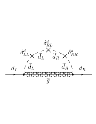
Figure 2: Additional GFM contributions to the diagonal elements of $m_{d}^{(0)}$.

It is possible in GFM models to induce large contributions to the bare down and strange quark masses through diagrams involving three insertions (Fig. 2) [26]. For example,

$$\left(m_{d}^{(0)}\right)_{22}=\frac{m_{s}}{\left(1+\epsilon_{s}\tan\beta\right)}\left[1-\frac{m_{b}}{m_{s}}\frac{\epsilon_{4}\tan\beta x_{\widetilde{d}_{R}}x_{\widetilde{d}_{L}}}{\left(1+\epsilon_{3}\tan\beta\right)}\left(\delta_{LL}^{d}\right)_{32}\left(\delta_{RR}^{d}\right)_{23}\right],$$ (43)

where $\epsilon_{4}$ is given by

$$\epsilon_{4}=-\frac{\alpha_{s}}{2\pi}C_{2}(3)\frac{\mu}{m_{\widetilde{g}}}H_{4}\left(x_{\widetilde{d}_{R}},x_{\widetilde{d}_{L}},x_{\widetilde{d}_{R}},x_{\widetilde{d}_{L}}\right).$$ (44)

The loop function $H_{4}$ is given in appendix A.1 whilst its arguments are given in (42).

Now let us turn to the off–diagonal elements of $m_{d}^{(0)}$. The diagrams in Fig. 1 and Fig. 3 illustrate the flavour violating corrections that arise from MFV and GFM contributions. Evaluating all four diagrams, we find the contribution

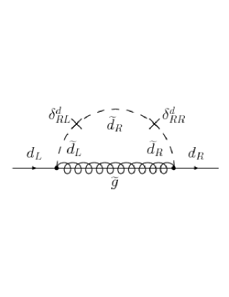
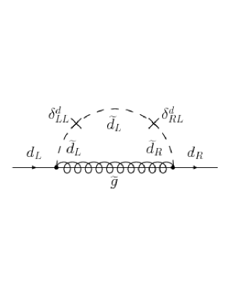
Figure 3: GFM contributions to the off–diagonal elements of $m_{d}^{(0)}$.

$$\left(m_{d}^{(0)}\right)_{ij} =\frac{\epsilon_{RL}x_{\widetilde{d}_{RL}}m_{\widetilde{g}}}{1+\epsilon_{j}\tan\beta}\left(\delta_{RL}^{d}\right)_{ij}-\frac{\epsilon_{RR}x_{\widetilde{d}_{R}}\left(m_{d}\right)_{jj}\tan\beta}{\left(1+\epsilon_{j}\tan\beta\right)^{2}}\left(\delta_{RR}^{d}\right)_{ij}$$

$$-\frac{\big{[}\epsilon_{LL}x_{\widetilde{d}_{L}}\left(\delta_{LL}^{d}\right)_{ij}+\epsilon_{Y}Y_{t}^{2}K_{ti}^{\ast}K_{tj}\big{]}\left(m_{d}\right)_{ii}\tan\beta}{\left(1+\epsilon_{i}\tan\beta\right)\left(1+\epsilon_{j}\tan\beta\right)},$$ (45)

where $\epsilon_{RL}$ and $\epsilon_{LL}$ are given by

$$\epsilon_{RL} =-\frac{\alpha_{s}}{2\pi}C_{2}\left(3\right)H_{2}\left(x_{\widetilde{d}_{R}},x_{\widetilde{d}_{L}}\right), \epsilon_{LL} =-\frac{\alpha_{s}}{2\pi}C_{2}(3)\frac{\mu}{m_{\widetilde{g}}}H_{3}\left(x_{\widetilde{d}_{R}},x_{\widetilde{d}_{R}},x_{\widetilde{d}_{L}}\right)$$ (46)

and $\epsilon_{RR}$ can be obtained by making the substitution $L\leftrightarrow R$ in the formula for $\epsilon_{LL}$. The loop functions $H_{2}$ and $H_{3}$ are defined in appendix A.1, the CKM matrix $K$ is defined in (11), $\epsilon_{i}$ and $\epsilon_{j}$ are defined in (39), and $x_{\widetilde{d}_{RL}}$ is given by

$$x_{\widetilde{d}_{RL}} =\frac{\sqrt{m_{d,LL}^{2}m_{d,RR}^{2}}}{m_{\widetilde{g}}^{2}}.$$ (47)

It will be useful to see how the above expressions behave in the limit of degenerate sparticle masses. For instance, the various $\epsilon$–factors that appear in the above formulae become

$$\epsilon_{s}= \frac{\alpha_{s}}{3\pi}sgn\left({\mu}\right), \epsilon_{Y}= \frac{1}{32\pi^{2}}sgn\left(\frac{A_{t}}{\mu}\right),$$ (48)

$$\epsilon_{G}= \frac{\alpha_{s}}{18\pi}sgn\left(\mu\right), \epsilon_{RL}= \frac{\alpha_{s}}{3\pi}, \epsilon_{LL}= -\frac{\alpha_{s}}{9\pi}sgn\left(\mu\right).$$ (49)

From (48) it is easy to see that, in the phenomenologically favoured region $\mu>0$, $A_{t}<0$, the chargino and gluino contributions in (39) for $i=3$ partially cancel. This can lead to a reduction of BLO contributions compared to a case where only gluino contributions are taken into account.

As we are chiefly concerned with flavour violation in the down squark sector, we can safely omit the effects induced by LR, RL and RR mixings amongst the up squarks. In other words we assume that $m^{2}_{u,LR}$ and $m^{2}_{u,RR}$ are diagonal matrices. However, the insertion $\delta_{LL}^{u}$ is related by ${\rm SU}(2)$ symmetry to $\delta_{LL}^{d}$ and its effects on the bare mass matrix should be included. In the approximation used in this subsection however, the contributions proportional to $\delta_{LL}^{u}$, that arise solely from higgsino exchange, are rather small, as they are suppressed by factors of the Yukawa couplings of the first two generations. We will see in section 3.3 however, that, once one includes the effects induced by non–zero electroweak couplings, additional contributions are possible.

3.2 Corrections to Electroweak Vertices in the MIA

Now let us consider the effect of supersymmetric contributions to the various electroweak vertices in the MIA. As stated in section 2.2, the CKM matrix that appears, for example, in the chargino vertex (35)–(37) is related to the physical CKM matrix by the relation (26). At first order in the MIA, the vertex and self energy corrections arising from gluino exchange cancel due to ${\rm SU}(2)_{L}\times{\rm U}(1)_{Y}$ gauge symmetry. The first corrections to $K$ therefore appear at second order, through diagrams involving two ${\rm SU}(2)_{L}\times{\rm U}(1)_{Y}$ breaking insertions on one of the squark lines. The contributions to the vertex therefore tend to be suppressed by factors of either $m_{b}$ or $\cot\beta$ and, whilst we take into account these effects in our numerical analysis, to a good approximation we may set $K=K^{\rm eff}$. A similar result holds for the effective right handed coupling of the $W$ boson (25).

Turning to the $Z$ boson vertex, once again we find that, to first order in the MIA, the self energy and vertex corrections cancel due to ${\rm SU}(2)_{L}\times{\rm U}(1)_{Y}$ gauge symmetry The first non–zero contribution arises from the diagram shown in Fig. 4 involving two ${\rm SU}(2)_{L}\times{\rm U}(1)_{Y}$ breaking insertions.

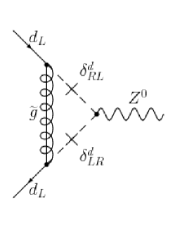
Figure 4: The gluino correction to the Z boson vertex that arises at second order in the MIA.

Evaluating the contributions to the effective vertex we find for $\left(C_{L}^{Z}\right)_{23}$

$$\left(C_{L}^{Z}\right)_{23}=-\frac{g_{2}}{2\cos\theta_{W}}\frac{\alpha_{s}C_{2}\left(3\right)}{2\pi}\frac{f_{Z}\left(x_{\widetilde{d}}\right)}{m_{\widetilde{g}}^{2}\left(1+\epsilon_{s}\tan\beta\right)}\left[\left(m_{d,LR}\right)_{33}-\frac{m_{b}\mu\tan\beta}{1+\epsilon_{3}\tan\beta}\right]\left(\delta_{LR}^{d}\right)_{23},$$ (50)

where the function $f_{Z}$ is given in appendix A.3. The expression in square brackets in the above expression represents the effect of the flavour diagonal RL insertion. The off–diagonal elements of the bare mass matrix can also induce terms proportional to $\delta_{LL}^{d}$ and $\delta_{RR}^{d}$, that can viably compete with the corresponding contributions that arise at third order in the MIA. Although the vertex (50) is enhanced by $\tan\beta$, we shall see later that the contributions to a given process due to this vertex scale as $m_{Z}^{2}/M_{SUSY}^{2}$ and are typically rather small.

Now let us turn to the Higgs sector, where the effects induced by supersymmetric contributions to the charged and neutral Higgs couplings are known to be large [11, 12, 24]. These corrections can, in turn, affect FCNC processes especially in regions of parameter space where FCNC mediated solely by sparticle exchange are suppressed by large sparticle masses.

The charged Higgs vertex receives corrections [25, 11, 12] from both gluino and higgsino exchange. To second order in the MIA, the effective charged Higgs coupling is given by

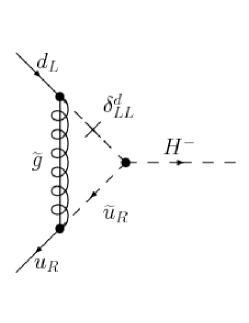
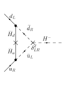
Figure 5: The dominant GFM contributions to the left–handed charged Higgs vertex, arising from gluino and higgsino exchange.

$$\left(C_{L}^{H^{+}}\right)_{ij}= \frac{g_{2}}{\sqrt{2}m_{W}}\left(m_{u}\right)_{ii}\cot\beta\left[K_{ij}\left(1-\epsilon_{s}^{\prime}\tan\beta+\epsilon_{Y}^{\prime}(Y_{b}^{(0)})^{2}\delta_{3j}\tan\beta\right)+\Lambda_{ij}^{L}\right],$$ (51)

$$\left(C_{R}^{H^{+}}\right)_{ij}= \frac{g_{2}}{\sqrt{2}m_{W}}\frac{\left(m_{d}\right)_{jj}}{\left(1+\epsilon_{i}\tan\beta\right)}\tan\beta\left(K_{ij}+\Lambda_{ij}^{R}\right),$$ (52)

where $i,j=1,2,3$ and $Y_{b}^{(0)}=(Y_{d}^{(0)})_{33}$. The factors $\epsilon_{s}^{\prime}$ and $\epsilon_{Y}^{\prime}$ are given by

$$\epsilon_{s}^{\prime} =-\frac{\alpha_{s}}{2\pi}C_{2}(3)\frac{\mu}{m_{\widetilde{g}}}H_{2}\left(x_{\widetilde{u}_{R}},x_{\widetilde{d}_{L}}\right), \epsilon_{Y}^{\prime} =-\frac{1}{16\pi^{2}}\frac{\left(m_{d,LR}\right)_{33}}{\mu\left(m_{d}^{(0)}\right)_{33}}H_{2}\left(y_{\widetilde{u}_{L}},y_{\widetilde{d}_{R}}\right).$$ (53)

The arguments of the loop functions $H_{2}$ can be obtained by the appropriate generalisations of (42). Finally, the $3\times 3$ matrices $\Lambda_{ij}^{L,R}$ denote the additional off–diagonal contributions that arise in both MFV and GFM models due to the off–diagonal elements of the bare mass matrix and the GFM parameters. $\Lambda_{ij}^{L,R}$ may be decomposed as follows

$$\Lambda_{ij}^{L,R}=\Delta_{ij}^{L,R}+\gamma_{ij}^{L,R}.$$ (54)

The MFV contributions $\Delta_{ij}^{L}$ to the vertex have been highlighted in [3, 14]. In the formalism developed in section 2, they arise due to the presence of the bare mass matrix in the neutralino vertex, and have the following form

$$\Delta_{ij}^{L}= K_{ij}\frac{\epsilon_{Y}^{\prime}\epsilon_{Y}(Y_{b}^{(0)}Y_{t}\tan\beta)^{2}}{1+\epsilon_{j}\tan\beta}, (i,j)=(3,1),(3,2),$$ (55)

$$\Delta_{ij}^{L}= 0, {\rm otherwise}.$$ (56)

It should be noted that the additional terms found in [14] for $(i,j)=(1,3),(2,3)$ do not appear as we do not assume that the trilinear soft terms are proportional to the bare Yukawa coupling. If one adopts the parameterisation described in appendix B, where such a relation is assumed, it can be shown that one obtains an additional contribution to $\Delta_{ij}^{L}$ in agreement with [14].

The GFM contributions to $\Lambda_{ij}^{L}$ arise from the two diagrams shown in Fig. 5. Evaluating the contributions yields

$$\gamma_{ij}^{L}= -K_{ii}\tan\beta\Bigg{[}\Bigg{(}\epsilon_{LL}^{\prime}-\frac{\epsilon_{LL}\epsilon_{Y}^{\prime}(Y_{b}^{(0)})^{2}\tan\beta}{1+\epsilon_{j}\tan\beta}\Bigg{)}x_{\widetilde{d}_{L}}\left(\delta_{LL}^{d}\right)_{ji}$$

$$+\frac{m_{\widetilde{g}}}{m_{b}}\frac{\epsilon_{RL}\epsilon_{Y}^{\prime}(Y_{b}^{(0)})^{2}x_{\widetilde{d}_{RL}}\left(1+\epsilon_{3}\tan\beta\right)}{\left(1+\epsilon_{j}\tan\beta\right)}\left(\delta_{LR}^{d}\right)_{ji}$$

$$+\epsilon_{RL}^{\prime}(Y_{b}^{(0)})(Y_{d}^{(0)})_{jj}y_{\widetilde{d}_{RL}}\left(\delta_{RL}^{d}\right)_{ji}\Bigg{]}, (i,j)=(3,1),(3,2),$$ (57)

$$\gamma_{ij}^{L}= -K_{ii}\tan\beta\left[\epsilon_{LL}^{\prime}x_{\widetilde{d}_{L}}\left(\delta_{LL}^{d}\right)_{ij}+\epsilon_{RL}^{\prime}(Y_{b}^{(0)})^{2}y_{\widetilde{d}_{RL}}\left(\delta_{LR}^{d}\right)_{ij}\right], (i,j)=(1,3),(2,3),$$ (58)

where $\epsilon_{LL}^{\prime}$ and $\epsilon_{RL}^{\prime}$ are

$$\epsilon_{LL}^{\prime} =-\frac{\alpha_{s}}{2\pi}C_{2}(3)\frac{\mu}{m_{\widetilde{g}}}H_{3}\left(x_{\widetilde{u}_{R}},x_{\widetilde{d}_{L}},x_{\widetilde{d}_{L}}\right), \epsilon_{RL}^{\prime} =-\frac{1}{16\pi^{2}}\frac{\mu}{\left(m_{d}^{(0)}\right)_{33}}H_{2}\left(y_{\widetilde{u}_{L}},y_{\widetilde{d}_{R}}\right).$$ (59)

It should be noted that the third term in (57) is proportional the Yukawa coupling of the down or strange quark. We include it however as the factors of $\cos\beta$ present in the denominators of the Yukawa couplings (we remind the reader that $Y_{d}\sim m_{d}/m_{W}\cos\beta$) can effectively lead $\gamma^{L}_{ij}$ to vary as $\tan^{3}\beta$. This term can become important if $\left(\delta_{LR}^{d}\right)_{32}=\delta_{RL}^{d}$ is large $\mathcal{O}\left(10^{-2}\right)$.

Now consider the right–handed coupling of the charged Higgs. In this case the dominant corrections to the vertex are due to the self–energy correction $\Sigma_{mL}^{d}$. The MFV contributions to the vertex are reflected by the appearance of a factor of $\left(1+\epsilon_{i}\tan\beta\right)$ in the denominator of (52), in agreement with [14].

In models with GFM it is possible to generate additional terms of the form

$$\gamma_{ij}^{R}=-K_{ii}\bigg{[} \frac{\epsilon_{RR}x_{\widetilde{d}_{R}}\tan\beta}{\left(1+\epsilon_{i}\tan\beta\right)}\frac{\left(m_{d}\right)_{ii}}{\left(m_{d}\right)_{jj}}\left(\delta_{RR}^{d}\right)_{ij}$$

$$+\epsilon_{RL}x_{\widetilde{d}_{RL}}\epsilon_{i}\frac{m_{\widetilde{g}}}{\left(m_{d}\right)_{jj}}\left(\delta_{RL}^{d}\right)_{ji}\bigg{]}, (i,j)=(3,1),(3,2),$$ (60)

$$\gamma_{ij}^{R}=-K_{ii}\bigg{[} \frac{\epsilon_{LL}x_{\widetilde{d}_{L}}\tan\beta}{\left(1+\epsilon_{j}\tan\beta\right)}\left(\delta_{LL}^{d}\right)_{ij}$$

$$+\epsilon_{RL}x_{\widetilde{d}_{RL}}\epsilon_{i}\frac{m_{\widetilde{g}}}{\left(m_{d}\right)_{jj}}\left(\delta_{LR}^{d}\right)_{ij}\bigg{]}, (i,j)=(1,3),(2,3).$$ (61)

A particularly interesting consequence of (60) is that one can often avoid the factor of the strange quark mass, that appears in the right handed vertex (51) when $i=3$ and $j=2$, via flavour violation in either the RL or RR sectors.

It is apparent from the above expressions that GFM contributions, to both the left and right–handed vertices, can play the rôle of the off–diagonal elements of the CKM matrix. The off–diagonal BLO corrections to the charged Higgs vertex can therefore be rather large in the GFM scenario. Substantial enhancement or suppression of charged Higgs contributions to FCNC are therefore possible, even in the limit where the squarks decouple from the theory. In addition, $\tan\beta$ enhanced corrections affect the underlying structure of the charged Higgs vertex, in both GFM and MFV, via the factors of $\left(1+\epsilon_{i}\tan\beta\right)$ that occur in the denominator in (52) and the corrections $\epsilon_{s}^{\prime}$ and $\epsilon_{Y}^{\prime}$ that appear in (51).

The corrections to the charged Goldstone boson vertex [11] prove to be rather small, as the vertex is protected by ${\rm SU}(2)$ symmetry and the self energy and vertex contributions approximately cancel. These cancellations are required as, in a general $R_{\xi}$ gauge, the corrected Goldstone boson vertex must act to cancel the $\xi$ dependence of the contributions originating from $W$ boson exchange. The corrected vertex must therefore, in a similar manner to the corrected $W$ boson vertex, be proportional to ${\rm SU}(2)_{L}\times{\rm U}(1)_{Y}$ breaking effects, even for GFM.

Finally, let us consider the corrected neutral Higgs vertices (33)–(34). The dominant contributions originate from the self energy corrections $\Sigma^{d}_{m\,L}$. To first order in the MIA the contributions to the flavour diagonal elements of the effective $A^{0}$ vertex become

$$\left(C^{A^{0}}_{L}\right)_{ii}= -\frac{ig_{2}}{2m_{W}}\tan\beta\frac{\left(m_{d}\right)_{ii}}{\left(1+\epsilon_{i}\tan\beta\right)},$$ (62)

whilst the contributions to the effective $H^{0}$ and $h^{0}$ vertices are

$$\left(C^{H^{0}}_{L}\right)_{ii}= -\frac{g_{2}}{2\cos\beta m_{W}}\frac{\left(m_{d}\right)_{ii}}{\left(1+\epsilon_{i}\tan\beta\right)}\left(\cos\alpha+\epsilon_{i}\sin\alpha\right),$$ (63)

$$\left(C^{h^{0}}_{L}\right)_{ii}= +\frac{g_{2}}{2\cos\beta m_{W}}\frac{\left(m_{d}\right)_{ii}}{\left(1+\epsilon_{i}\tan\beta\right)}\left(\sin\alpha-\epsilon_{i}\cos\alpha\right).$$ (64)

At third order in the MIA, further corrections proportional to combinations of $\delta_{LL}^{d}$ and $\delta_{RR}^{d}$ are generated in a similar manner to (43) that can lead to large corrections to the Yukawa couplings of the first two generations. Full expressions can be found in [26].

The off–diagonal elements of the coupling are generated by MFV and GFM contributions and, in a similar manner to the charged Higgs vertex, it is useful to perform the decomposition

$$\left(C_{L,R}^{S^{0}}\right)_{ij}=\left(C_{L,R}^{S^{0}}\right)^{\rm MFV}_{ij}+\left(C_{L,R}^{S^{0}}\right)^{\rm GFM}_{ij},$$ (65)

where $S^{0}=A^{0},G^{0},H^{0},h^{0}$. The dominant MFV contributions to the off–diagonal elements of the coupling arise from higgsino exchange and are given by [3, 14],

$$\left(C_{L}^{A^{0}}\right)^{\rm MFV}_{ij}=\frac{ig_{2}}{2m_{W}}\frac{\left(m_{d}\right)_{ii}\epsilon_{Y}Y_{t}^{2}K_{ti}^{\ast}K_{tj}\tan^{2}\beta}{\left(1+\epsilon_{i}\tan\beta\right)\left(1+\epsilon_{j}\tan\beta\right)}.$$ (66)

The GFM contributions arise primarily from gluino exchange and yield the additional contribution

$$\left(C_{L}^{A^{0}}\right)^{\rm GFM}_{ij}=\frac{ig_{2}}{2m_{W}}\tan^{2}\beta\Bigg{[} \frac{\left(m_{d}\right)_{ii}\epsilon_{LL}x_{\widetilde{d}_{L}}}{\left(1+\epsilon_{i}\tan\beta\right)\left(1+\epsilon_{j}\tan\beta\right)}\left(\delta_{LL}^{d}\right)_{ij}$$

$$+\frac{\epsilon_{RL}\epsilon_{j}m_{\widetilde{g}}x_{\widetilde{d}_{RL}}}{\left(1+\epsilon_{j}\tan\beta\right)}\left(\delta_{RL}^{d}\right)_{ij}+\frac{\left(m_{d}\right)_{jj}\epsilon_{RR}x_{\widetilde{d}_{R}}}{\left(1+\epsilon_{j}\tan\beta\right)^{2}}\left(\delta_{RR}^{d}\right)_{ij}\Bigg{]}.$$ (67)

The off–diagonal couplings of the scalar Higgs bosons $H^{0}$ and $h^{0}$ may be obtained via the simple substitutions

$$C_{L}^{H^{0}}= \;i\sin\left(\alpha-\beta\right)C_{L}^{A^{0}}, C_{L}^{h^{0}}= \;i\cos\left(\alpha-\beta\right)C_{L}^{A^{0}},$$ (68)

whilst the right handed couplings can be obtained by taking the Hermitian conjugate. Due to an accidental cancellation between the self–energy and vertex corrections, the terms proportional to $\delta_{RL}^{d}$ and $\delta_{LR}^{d}$ vanish at LO. However, once BLO corrections are taken into account, it is possible for these insertions to reappear through their effects on the bare mass matrix $m_{d}^{(0)}$ [17].

Once again, it should be noted that, due to ${\rm SU}(2)$ invariance, the Goldstone boson vertex does not receive large corrections even once GFM contributions are taken into account. As a result any contributions to the corrected vertex are attributable solely to ${\rm SU}(2)_{L}\times{\rm U}(1)_{Y}$ breaking effects and are rather small.

3.3 Additional Electroweak Effects

As discussed at the beginning of this section the results presented so far have been derived in the limit where the electroweak gauge couplings $g_{1}$ and $g_{2}$ are set equal to zero. The aim of this subsection is to briefly discuss the dominant contributions that arise once one proceeds beyond that approximation, and to provide some simple substitutions such that these effects can be taken into account.

First, let us consider the effect of such corrections on the bare mass matrix. One of the most important corrections in this case is due to the gaugino–higgsino mixing diagram shown in Fig. 6 that arises if the insertion $\delta_{LL}^{u}$ is non–zero [21].

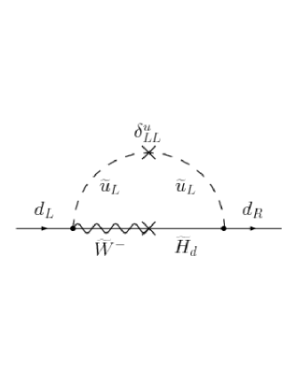
Figure 6: Contributions to $m_{d}^{(0)}$ arising from the insertion $\delta_{LL}^{u}$.

The corrections induced by this diagram may be taken into account by making the following substitution in (45)

$$\epsilon_{LL}x_{\widetilde{d}_{L}}\to\epsilon_{LL}x_{\widetilde{d}_{L}}+\sum_{a=1}^{2}\epsilon_{\chi\,LL}^{a}y_{\widetilde{d}_{L}}^{a},$$ (69)

where $y_{\widetilde{d}_{L}}^{a}=m_{d,LL}^{2}/m_{\chi^{-}_{a}}^{2}$ and $\epsilon^{a}_{\chi\,LL}$ is given by

$$\epsilon_{\chi\,LL}^{a}=\frac{\alpha}{4\pi\sin^{2}\theta_{W}}\frac{V_{a1}^{\ast}m_{\chi^{-}_{a}}U_{a2}}{\sqrt{2}m_{W}\sin\beta}H_{2}\left(y_{\widetilde{d}_{L}}^{a},y_{\widetilde{d}_{L}}^{a}\right).$$ (70)

$\alpha$ denotes the electromagnetic coupling constant. We have made use of the relation (22) to express the contribution in terms of flavour violation in the down squark sector. In the phenomenologically interesting region $\mu>0$ and $A_{t}<0$, $\epsilon^{a}_{\chi\,LL}$ interferes destructively with the gluino contribution $\epsilon_{LL}$ and acts to reduce the correction to $m_{d}^{(0)}$ that is proportional to flavour violation in the LL sector.

Turning to the charged Higgs vertex, as discussed in [14], large contributions to the left–handed vertex arise from diagrams featuring gaugino and higgsino exchange. They may be included by making the following substitution in (51)

$$\epsilon_{s}^{\prime}\to\epsilon_{s}^{\prime}+\epsilon_{\chi}^{\prime}.$$ (71)

$\epsilon_{\chi}^{\prime}$ has the following form

$$\epsilon_{\chi}^{\prime}= -\frac{\alpha}{4\pi\sin^{2}\theta_{W}}\sum_{a,\alpha}\frac{m_{\chi^{0}_{\alpha}}}{m_{\chi^{-}_{a}}}\overline{M}_{\alpha a}\bigg{\{}-\frac{2}{3}V_{a2}^{\ast}N_{\alpha 1}^{\ast}\tan\theta_{W}H_{2}\left(y_{\widetilde{u}_{R}}^{a},w_{\alpha}^{a}\right)$$

$$+\left[\frac{1}{2}V_{a2}^{\ast}\left(\frac{1}{3}N_{\alpha 1}^{\ast}\tan\theta_{W}-N_{\alpha 2}^{\ast}\right)-\frac{1}{\sqrt{2}}V_{a1}^{\ast}N_{\alpha 4}^{\ast}\right]H_{2}\left(y_{\widetilde{d}_{L}}^{a},w_{\alpha}^{a}\right)\bigg{\}},$$ (72)

where the quantity $\overline{M}_{\alpha a}$ is given by

$$\overline{M}_{\alpha a}=U_{a2}\left(N_{\alpha 1}^{\ast}\tan\theta_{W}+N_{\alpha 2}^{\ast}\right)-\sqrt{2}U_{a1}N_{\alpha 3}^{\ast}.$$

Our results for $\epsilon_{\chi}^{\prime}$ agree with those originally given in [14]. To include the additional effects induced by GFM, one has to consider the diagrams shown in Fig. 7.

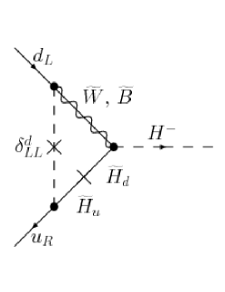
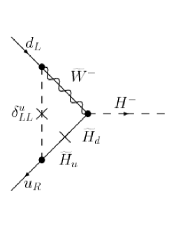
Figure 7: Additional GFM contributions to the left–handed charged Higgs vertex, due to the electroweak effects considered in subsection 3.3.

Their effects may be included by making the following correction to (57)–(58)

$$\epsilon_{LL}^{\prime}x_{\widetilde{d}_{L}}\to\epsilon_{LL}^{\prime}x_{\widetilde{d}_{L}}+\sum_{a}y_{\widetilde{d}_{L}}^{a}\epsilon^{a\;\prime}_{\chi\,LL},$$ (73)

where $\epsilon^{a\;\prime}_{\chi\;LL}$ is given by

$$\epsilon_{\chi\,LL}^{a\;\prime}= -\frac{\alpha}{4\pi\sin^{2}\theta_{W}}\sum_{\alpha}\frac{m_{\chi^{0}_{\alpha}}}{m_{\chi^{-}_{a}}}\overline{M}_{\alpha a}$$

$$\times\left[\frac{1}{2}V_{a2}^{\ast}\left(\frac{1}{3}N_{\alpha 1}^{\ast}\tan\theta_{W}-N_{\alpha 2}^{\ast}\right)-\frac{1}{\sqrt{2}}V_{a1}^{\ast}N_{\alpha 4}^{\ast}\right]H_{3}\left(y_{\widetilde{d}_{L}}^{a},y_{\widetilde{d}_{L}}^{a},w_{\alpha}^{a}\right).$$ (74)

Both the MFV (72) and GFM (74) corrections typically interfere destructively with the dominant gluino contributions and can lead to an appreciable reduction of BLO effects.

Finally, let us consider the neutral Higgs vertex. As discussed in the previous subsection, the dominant contributions to the effective vertex arise from the self–energy corrections $\Sigma^{d}_{mL}$. The effects induced by non–zero electroweak couplings may therefore be included, in a similar manner to the bare mass matrix, by making the substitution (69) in (67).

3.4 Other Methods

The method outlined in section 2 takes into account both $\tan\beta$ enhanced effects and those induced by non–minimal sources of flavour violation. Other methods have been proposed in the literature that can be modified to include the effects of GFM and it shall be useful to briefly consider how two specific examples compare with the method employed in this paper.

The first method, presented by Buras et al. [14], works in the bare SCKM basis. In this basis the Yukawa matrices $Y_{d}^{(0)}$ and $Y_{u}^{(0)}$ that appear in the superpotential are diagonal. Calculating the self–energies in this basis gives the physical quark masses

$$m_{d}=D_{R}\left(v_{d}\hat{Y}_{d}^{(0)}+\delta\hat{m}^{(0)}\right)D_{L}^{{\dagger}}$$ (75)

where $\hat{Y}_{d}^{(0)}$ is the diagonalised Yukawa matrix, and $\delta\hat{m}^{(0)}$ denotes the contributions of the self energy corrections (5) calculated in the bare SCKM basis. $D_{L}$ and $D_{R}$ denote the unitary transformations performed on the squark fields that transform between the bare and physical SCKM bases. The bare mass matrix $m_{d}^{(0)}$ defined in (3) is related to these quantities by

$$m_{d}^{(0)}=D_{R}\left(v_{d}\hat{Y}_{d}^{(0)}\right)D_{L}^{{\dagger}}.$$ (76)

It is straightforward to relate the matrices $D_{L,R}$ to the unitary matrices $V_{d_{L,R}}$ that appeared in section 2. If, in analogy with the transformations (8)–(9), one defines a transformation from the interaction basis to the bare SCKM basis such that

$$\hat{Y}_{d}^{(0)}=V_{d_{R}}^{(0)}\left(Y_{d}^{(0)o}\right)V_{d_{L}}^{(0){\dagger}}.$$ (77)

$D_{R}$ and $D_{L}$ are then given by

$$D_{L} =V_{d_{L}}V_{d_{L}}^{(0){\dagger}}, D_{R} =V_{d_{R}}V_{d_{R}}^{(0){\dagger}}.$$ (78)

One may also define the bare CKM matrix in the SCKM basis

$$K^{(0)}=V_{u_{L}}^{(0)}V_{d_{L}}^{(0){\dagger}}=U_{L}^{{\dagger}}KD_{L}.$$ (79)

The rôle played by the off–diagonal elements of $m_{d}^{(0)}$ in section 2 is taken by the unitary matrices $D_{L}$, $D_{R}$ and the bare CKM matrix $K^{(0)}$. For instance, the bare CKM matrix elements $K^{(0)}_{ts}$ and $K^{(0)}_{cb}$, in the bare SCKM basis, are related to the corresponding matrix elements K, defined in the physical SCKM basis via the relation

$$K_{ts}^{(0)}= \frac{\left(1+\epsilon_{3}\tan\beta\right)}{\left(1+\epsilon_{s}\tan\beta\right)}K_{ts}-\left[\epsilon_{RL}\frac{\left(1+\epsilon_{3}\tan\beta\right)}{\left(1+\epsilon_{s}\tan\beta\right)}\frac{m_{\widetilde{g}}}{m_{b}}x_{\widetilde{d}_{RL}}\delta_{LR}^{d}-\frac{\epsilon_{LL}\tan\beta}{\left(1+\epsilon_{s}\tan\beta\right)}x_{\widetilde{d}_{L}}\delta_{LL}^{d}\right]K_{tb},$$ (80)

$$K_{cb}^{(0)}= \frac{\left(1+\epsilon_{3}\tan\beta\right)}{\left(1+\epsilon_{s}\tan\beta\right)}K_{cb}+\left[\epsilon_{RL}\frac{\left(1+\epsilon_{3}\tan\beta\right)}{\left(1+\epsilon_{s}\tan\beta\right)}\frac{m_{\widetilde{g}}}{m_{b}}x_{\widetilde{d}_{RL}}\delta_{LR}^{d}-\frac{\epsilon_{LL}\tan\beta}{\left(1+\epsilon_{s}\tan\beta\right)}x_{\widetilde{d}_{L}}\delta_{LL}^{d}\right]K_{cs}.$$ (81)

Where we have used the shorthand $\delta_{LL}^{d}=\left(\delta_{LL}^{d}\right)_{23}$ and $\delta_{LR}^{d}=\left(\delta_{LR}^{d}\right)_{23}$. Strictly speaking, the uncorrected CKM matrix $K$ should appear in the above relations, however, as discussed in section 3.2, the vertex and self energy corrections are negligible and one may, to a good approximation, set $K=K^{\rm eff}$. An interesting consequence of this formula is that the matrix element $K_{ts}^{(0)}$ obtained by diagonalising the bare Yukawa couplings $Y_{d,u}^{(0)o}$ can be zero in the presence of general flavour mixing [21, 16]. We will discuss the consequences of this in section 7.4.

As the two methods are practically equivalent, choosing between them essentially becomes a choice as to which is more suitable for the problem at hand. In MFV scenarios the method presented in [14] is generally more convenient as it is only necessary to calculate the diagonal parts to the vertex and self–energy corrections induced by gluino exchange. For example, when using the method described in section 2 the correct form of (66) is only obtained when one considers the off–diagonal gluino contributions as well as the higgsino exchange diagram.

In the GFM scenario the situation is rather different. As the off–diagonal contributions to the electroweak vertices and non–renormalizable operators induced by gluino exchange are evaluated anyway, the method described in this paper can become more preferable. In particular, the flavour diagonal contributions, induced by the exchange of the supersymmetric particles, to the various non–renormalizable operators applicable to the process under investigation no longer have to be calculated, as the rôle played by the matrices $D_{L}$ and $D_{R}$ is replaced by the off–diagonal elements of $m_{d}^{(0)}$.

The second method, presented by Dedes and Pilaftsis [13], concerns itself mainly with CP violation, however it is essentially applicable to both MFV and GFM CP conserving scenarios as well. After translating to the physical SCKM basis their expression for the bare mass matrix reads

$$m_{d}=m_{d}^{(0)}R,$$ (82)

where $R$ is a $3\times 3$ matrix. It is then possible to express the various Higgs interactions via an effective Lagrangian expressed in terms of the physical quark masses and the inverse of $R$. In the context of MFV and GFM scenarios with mixing only in the LL sector this parameterisation is sufficient. However taking into account all sources of flavour violation yields the more general form

$$m_{d}=m_{d}^{(0)}R_{L}+R_{R}m_{d}^{(0)}+R_{G}.$$ (83)

In the MIA, the $3\times 3$ matrices $R_{L}$, $R_{R}$ and $R_{G}$ may be decomposed in the following way

$$R_{L} ={\mathchoice{\rm 1\mskip-4.0mul}{\rm 1\mskip-4.0mul}{\rm 1\mskip-4.5mul}{\rm 1\mskip-5.0mul}}+\epsilon_{s}\tan\beta+\sum_{u}\epsilon_{Y}K^{{\dagger}}Y_{u}^{2}K\tan\beta+\epsilon_{LL}\tan\beta\;x_{\widetilde{d}_{L}}\delta_{LL}^{d},$$

$$R_{R} =+\epsilon_{RR}\tan\beta\;x_{\widetilde{d}_{R}}\delta_{RR}^{d},$$ (84)

$$R_{G} =-\epsilon_{RL}\;m_{\widetilde{g}}x_{\widetilde{d}_{RL}}\delta_{RL}^{d}.$$

Obtaining a solution for $m_{d}^{(0)}$ is therefore rather more complicated than simply finding the inverse of $R$. Considering each element of $m_{d}^{(0)}$ in turn, however, it is possible to replicate the results for $m_{d}^{(0)}$ presented in subsection 3.1.

4 $\bar{B}\to X_{s}\gamma$ Beyond the LO

Of all the FCNC processes involving transitions between the $b$ and $s$ quarks, $\bar{B}\to X_{s}\gamma$ is currently the best understood both experimentally and theoretically. The data being taken by B–factories such as BaBar and BELLE, is leading to an increasing degree of precision for the measurement of the branching ratio of the decay. The current world average is [27]

$${\rm BR}\left(\bar{B}\to X_{s}\gamma\right)_{\rm exp}=\left(3.39^{+0.30}_{-0.27}\right)\times 10^{-4}.$$ (85)

This value takes into account the most recent BELLE [28] and BaBar results [29].

The SM prediction for the branching ratio is based on a NLO calculation that was completed in Refs. [30, 31, 32], resulting in the prediction

$${\rm BR}\left(\bar{B}\to X_{s}\gamma\right)_{\rm SM}=\left(3.70\pm 0.30\right)\times 10^{-4}.$$ (86)

It has been pointed out recently [33] that, if one applies a realistic cut–off for the photon energy (rather than $E_{\gamma}>1/20\;m_{b}$), a dependence on two additional energy scales appears when calculating the branching ratio for the decay. The first scale ($\mu_{i}=\sqrt{m_{b}\Delta}$) is associated with the energy of the final hadronic state $X_{s}$, whilst the second is dependent on the energy range under investigation ($\mu_{0}=\Delta=m_{b}-2E_{\gamma}$). The perturbative uncertainties associated with these scales are rather large and can lead to a significant increase in the error associated with the branching ratio. However, in exchange, the final result can be compared directly with those determined directly from experiment rather than model dependent extrapolations to $E_{\gamma}>1/20\;m_{b}$.

We should also briefly mention that steps are now being taken towards a NNLO calculation [34, 35], that should increase the accuracy of the SM prediction to roughly 5%.

The effective Hamiltonian relevant to $\Delta F=1$ processes such as the decay $\bar{B}\to X_{s}\gamma$ is

$$\mathcal{H}_{eff}=-\frac{4G_{F}}{\sqrt{2}}K^{\rm eff}_{ts}{}^{\ast}K^{\rm eff}_{tb}\sum_{i=1}^{8}\left[C_{i}\left(\mu\right)\mathcal{O}_{i}\left(\mu\right)+C_{i}^{\prime}\left(\mu\right)\mathcal{O}_{i}^{\prime}\left(\mu\right)\right].$$ (87)

The operators most relevant to the decay are

$$\mathcal{O}_{7} =\frac{e}{16\pi^{2}}m_{b}\left(\overline{s}_{L}\sigma^{\mu\nu}b_{R}\right)F_{\mu\nu}, \mathcal{O}_{8} =\frac{g_{s}}{16\pi^{2}}m_{b}\left(\overline{s}_{L}\sigma^{\mu\nu}T^{a}b_{R}\right)G_{\mu\nu}^{a}.$$ (88)

(The six remaining operators can be found, for example, in [30]). The primed operators can be obtained via the simple substitution $L\leftrightarrow R$. The contributions to the primed operators are negligible in the SM. However, in more general models, such as the MSSM with general flavour mixing, their effects can no longer be ignored. As the primed and unprimed operators do not interfere with one another, any new physics contributions to $C_{7}^{\prime}$ and $C_{8}^{\prime}$ enter quadratically and therefore act to increase the value of the branching ratio. New physics contributions to $C_{7}$ and $C_{8}$, on the other hand, interfere directly with the SM contribution and can lead to far more varied effects.

The good agreement (within $1\sigma$) of the SM prediction and the current experimental results allows one to place increasingly stringent bounds on the effects and mass scale of new physics contributions. In doing so it is important to include the effects of new physics at a similar precision to the SM result. NLO matching conditions have been completed for several extensions of the SM, for example, the NLO matching conditions relevant to the 2HDM were presented in [37, 36] whilst a more general analysis was presented in [38]. Turning to the MSSM, however, things become rather more complicated. A complete NLO calculation would involve the evaluation two loop diagrams involving both gluons and gluinos. For MFV this task is already underway and, for example, the NLO matching conditions for the charged Higgs contribution have been discussed in [39]. Theoretical calculations have, thus far, concentrated on particular cases. The calculation presented in [40], for example, considers a realistic but specific region of MSSM parameter space where the charginos and lightest stop are relatively light compared to the rest of the sparticle spectrum and $\tan\beta$ is rather small. These results were extended to the large $\tan\beta$ regime in [11, 12]. The same papers also considered the dominant effects that occur BLO for generic SUSY scenarios taking into account effects enhanced by large logs and $\tan\beta$. These results were subsequently extended to include CP violation [41], additional CKM effects [3] and ${\rm SU}(2)_{L}\times{\rm U}(1)_{Y}$ breaking and electroweak effects in [14].

In the GFM scenario the LO matching conditions have been known for some time [42, 43, 44] and, in a similar manner to the MFV calculation, the NLO matching conditions have been derived in the limit where the gluino decouples and $\tan\beta$ is small [38]. An extension of the analysis given in [11] to the GFM scenario was presented in [15, 16] where it was found that BLO corrections can play a large rôle and can lead to a significant relaxation of the limits placed on GFM parameters compared to a LO analysis. The aim of this section is to present calculations in the MIA for both the electroweak and SUSY contributions to $\bar{B}\to X_{s}\gamma$, allowing one to easily determine the dominant effects that occur once GFM is taken into account compared to MFV calculations, as well as presenting the calculations detailed in [16] in a more transparent way. In doing so we therefore adopt the approximations discussed at the beginning of section 3.

4.1 BLO Corrections to Electroweak Contributions in the MIA

As emphasised in section 2, including $\tan\beta$ enhanced corrections to the charged and neutral Higgs vertices can lead to large effects. Let us first consider how the LO charged Higgs contributions to the decay $\bar{B}\to X_{s}\gamma$ are altered once these effects are taken into consideration. Using the corrected vertices (51)–(52) the dominant MFV contribution in the large $\tan\beta$ regime is given by [11, 3, 14]

$$\left(\delta^{H^{-}}C_{7,8}\right)^{\rm MFV} =\frac{1}{1+\epsilon_{3}\tan\beta}\left(1-\epsilon_{s}^{\prime}\tan\beta+\frac{\epsilon_{Y}^{\prime}\epsilon_{Y}(Y_{b}^{(0)}Y_{t}\tan\beta)^{2}}{1+\epsilon_{s}\tan\beta}\right)F_{7,8}^{(2)}\left(\frac{m_{t}^{2}}{m_{H^{+}}^{2}}\right).$$ (89)

The loop function $F_{7,8}^{(2)}$ is given in appendix A.2. Note that (89) includes the LO contribution in addition to the BLO corrections. Turning to the degenerate mass limit we see that $\epsilon_{s}^{\prime}$ depends on the sign of $\mu$. In the phenomenologically favoured region $\mu>0$, for example, the BLO corrections induced by gluino exchange typically reduce the branching ratio compared to a simple LO calculation. The higher order contribution proportional to $Y_{b}^{(0)2}$, first pointed out in [3], on the other hand is dependent on the sign of the trilinear soft terms and can therefore interfere destructively or constructively with the (dominant) gluino correction depending on the model at hand. It should be noted that (89) only serves as a rough approximation of the BLO effects and that the additional effects arising, for example, from gaugino mediated exchange and ${\rm SU}(2)_{L}\times{\rm U}(1)_{Y}$ breaking can lead to deviations from this idealised result in some regions of parameter space [14]. The dominant effects that arise from these corrections may be included by performing the substitutions presented in subsection 3.3.

The GFM contributions to the charged Higgs vertex, discussed in section 3.2, give rise to additional BLO corrections to $C_{7,8}$ given by

$$\left(\delta^{H^{-}}C_{7,8}\right)^{\rm GFM}=-\frac{K_{tb}^{\ast}}{K_{ts}^{\ast}}\Bigg{\{} \left[\frac{\epsilon_{LL}^{\prime}x_{\widetilde{d}_{L}}\tan\beta}{\left(1+\epsilon_{3}\tan\beta\right)}-\frac{\epsilon_{Y}^{\prime}\epsilon_{LL}x_{\widetilde{d}_{L}}(Y_{b}^{(0)}\tan\beta)^{2}}{\left(1+\epsilon_{s}\tan\beta\right)\left(1+\epsilon_{3}\tan\beta\right)}\right]\delta_{LL}^{d}$$

$$+\frac{m_{\widetilde{g}}}{m_{b}}\frac{\epsilon_{RL}\epsilon_{Y}^{\prime}x_{\widetilde{d}_{RL}}(Y_{b}^{(0)})^{2}\tan\beta}{1+\epsilon_{s}\tan\beta}\delta_{LR}^{d}$$

$$+\epsilon_{RL}^{\prime}y_{\widetilde{d}_{RL}}Y_{b}^{(0)}Y_{s}^{(0)}\tan\beta\;\delta_{RL}^{d}\Bigg{\}}F_{7,8}^{(2)}\left(\frac{m_{t}^{2}}{m_{H^{+}}^{2}}\right).$$ (90)

The factor of $K_{tb}^{\ast}/K_{ts}^{\ast}$ that appears in front of (90) reflects the fact that the flavour change is governed by the GFM parameters $\delta_{LL}^{d}$ and $\delta_{LR}^{d}$, rather than the CKM matrix. The additional GFM contributions interfere directly with the MFV corrections to the LO result and, depending on the sign of $\delta_{LL}^{d}$ or $\delta_{LR}^{d}$, can easily lead to large reductions or enhancements of the MFV result. In addition to these contributions to $C_{7,8}$ it is also possible, for non–zero $\delta_{RR}^{d}$ and $\delta_{RL}^{d}$, to induce corrections to the primed Wilson coefficients

$$\left(\delta^{H^{-}}C_{7,8}^{\prime}\right)^{\rm GFM}=-\bigg{[} \frac{m_{b}^{2}}{m_{t}^{2}}\frac{\tan^{2}\beta}{\left(1+\epsilon_{3}\tan\beta\right)^{2}}F_{7,8}^{(1)}\left(\frac{m_{t}^{2}}{m_{H^{+}}^{2}}\right)$$

$$+\frac{[1-(\epsilon_{s}^{\prime}+\epsilon_{Y}^{\prime}(Y_{b}^{(0)})^{2})\tan\beta]}{\left(1+\epsilon_{3}\tan\beta\right)}F_{7,8}^{(2)}\left(\frac{m_{t}^{2}}{m_{H^{+}}^{2}}\right)\bigg{]}$$

$$\times\frac{K_{tb}^{\ast}}{K_{ts}^{\ast}}\left[\frac{\epsilon_{RR}x_{\widetilde{d}_{R}}\tan\beta}{\left(1+\epsilon_{3}\tan\beta\right)}\delta_{RR}^{d}+\frac{m_{\widetilde{g}}}{m_{b}}\epsilon_{RL}\epsilon_{3}x_{\widetilde{d}_{RL}}\delta_{RL}^{d}\right].$$ (91)

As the LO contributions to the primed coefficients are suppressed by factors of $m_{s}/m_{b}$ the dominant behaviour, once BLO corrections are taken into account, is determined solely by GFM effects. Note that these GFM effects persist even if the squarks decouple from the theory.

It has been pointed out in Refs. [3, 14] that the corrected neutral Higgs vertex can also induce contributions to $C_{7,8}$ through the diagram where a neutral Higgs boson and a bottom quark undergoing a chirality flip are exchanged. In the limit of MFV using the corrected vertex (66) one obtains [3, 14]

$$\left(\delta^{H^{0}}C_{7,8}\right)^{\rm MFV}= -\frac{1}{36}\frac{m_{b}^{2}}{m_{A}^{2}}\tan^{3}\beta\frac{\epsilon_{Y}Y_{t}^{2}}{\left(1+\epsilon_{s}\tan\beta\right)\left(1+\epsilon_{3}\tan\beta\right)^{2}}.$$ (92)

The $\tan^{3}\beta$ dependence of the Wilson coefficient is characteristic of the corrected Higgs vertex (66) and can compensate for the suppression factor $m_{b}^{2}/m_{A}^{2}$.

Turning to the effects of GFM contributions, using (67) it is possible to induce additional corrections to $C_{7,8}$

$$\left(\delta^{H^{0}}C_{7,8}\right)^{\rm GFM}= -\frac{1}{36}\frac{m_{b}^{2}}{m_{A}^{2}K_{ts}^{\ast}K_{tb}}\tan^{3}\beta\Bigg{[}\frac{\epsilon_{LL}x_{\widetilde{d}_{L}}}{\left(1+\epsilon_{s}\tan\beta\right)\left(1+\epsilon_{3}\tan\beta\right)^{2}}\delta_{LL}^{d}$$

$$+\frac{m_{\widetilde{g}}}{m_{b}}\frac{\epsilon_{RL}x_{\widetilde{d}_{RL}}\epsilon_{s}}{\left(1+\epsilon_{s}\tan\beta\right)\left(1+\epsilon_{3}\tan\beta\right)}\delta_{LR}^{d}\Bigg{]}.$$ (93)

In a similar manner to (92), the GFM contributions arising from neutral Higgs exchange vary as $\tan^{3}\beta$. The primed coefficients also receive contributions if $\delta_{RL}^{d}$ or $\delta_{RR}^{d}$ are non zero

$$\left(\delta^{H^{0}}C_{7,8}^{\prime}\right)^{\rm GFM}= -\frac{1}{36}\frac{m_{b}^{2}}{m_{A}^{2}K_{ts}^{\ast}K_{tb}}\tan^{3}\beta\Bigg{[}\frac{\epsilon_{RR}x_{\widetilde{d}_{R}}}{\left(1+\epsilon_{3}\tan\beta\right)^{3}}\delta_{RR}^{d}$$

$$+\frac{m_{\widetilde{g}}}{m_{b}}\frac{\epsilon_{RL}\epsilon_{3}x_{\widetilde{d}_{RL}}}{\left(1+\epsilon_{3}\tan\beta\right)^{2}}\delta_{RL}^{d}\Bigg{]}.$$ (94)

4.2 BLO Corrections to SUSY Contributions in the MIA

The supersymmetric contributions to the decay $\bar{B}\to X_{s}\gamma$ can proceed through a number of channels. In MFV, the only SUSY contributions arise from diagrams involving chargino exchange. Once GFM effects are taken into account, additional diagrams arising from FCNC mediated by gluinos and neutralinos can occur and give rise to contributions to both the unprimed and primed Wilson coefficients. As the gluino contributions are enhanced by factors of $\alpha_{s}$ (compared to the MFV contributions), these effects are rather large and can play an important rôle for even small deviations from MFV.

All four insertions give rise to contributions to either $C_{7,8}$ or their primed counterparts and it will be useful, for our purposes, to decompose the overall gluino mediated contribution to the decay as follows

$$\delta^{\widetilde{g}}C_{7,8}=\left(\delta^{\widetilde{g}}C_{7,8}\right)^{\rm MFV}+\left(\delta^{\widetilde{g}}C_{7,8}\right)^{\rm LL}+\left(\delta^{\widetilde{g}}C_{7,8}\right)^{\rm LR}+\left(\delta^{\widetilde{g}}C_{7,8}\right)^{\rm RL}+\left(\delta^{\widetilde{g}}C_{7,8}\right)^{\rm RR}$$ (95)

The primed coefficients and other SUSY contributions may be defined in a similar manner. The dominant BLO corrections to the gluino contributions, shown in Fig. 8,

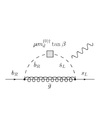
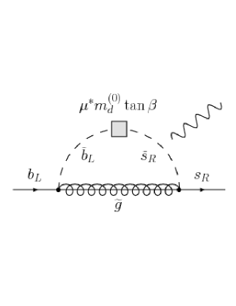
Figure 8: BLO corrections to $C_{7}$ ($C_{8}$) and $C_{7}^{\prime}$ ($C_{8}^{\prime}$) arising from gluino exchange, the photon (gluon) line is attached in every possible manner.

arise from the flavour violation mediated by the off–diagonal elements of the bare mass matrix and are proportional to $m_{d}^{(0)}\tan\beta$.

The MFV terms present in the bare mass matrix (45) can lead to a correction to the gluino contribution of the following form

$$\left(\delta^{\widetilde{g}}C_{7,8}\right)^{\rm MFV} =-\frac{8}{3}\frac{\alpha_{s}}{\alpha}\frac{\sin^{2}\theta_{W}m_{W}^{2}}{m_{\widetilde{g}}^{2}}\frac{\epsilon_{Y}Y_{t}^{2}\tan^{2}\beta}{\left(1+\epsilon_{s}\tan\beta\right)\left(1+\epsilon_{3}\tan\beta\right)}\frac{\mu}{m_{\widetilde{g}}}I_{6}^{[7,8]}\left(x_{\widetilde{d}}\right).$$ (96)

The loop functions $I_{i}^{[7,8]}\left(x\right)$ and $J_{i}^{[7,8]}\left(x\right)$, that appear throughout this section, can be found in appendix A.2, $x_{\widetilde{d}}$ denotes the ratio

$$x_{\widetilde{d}}=\frac{m_{\widetilde{q}}^{2}}{m_{\widetilde{g}}^{2}}$$ (97)

where $m_{\widetilde{q}}^{2}$ is a common mass of the quadratic soft terms (12) (that is, $m_{\widetilde{q}}^{2}=\left(m_{d,LL}^{2}\right)_{ii}=\left(m_{d,RR}^{2}\right)_{ii}$). Due to the $1/m_{\widetilde{g}}^{3}$ suppression of the amplitude it would be expected that these effects are typically rather small when compared to the additional BLO effects arising, for example, from the modified charged Higgs vertex. However, the terms feature a dependence on $\tan^{2}\beta$ in the numerator and should be included if one wants to consider the effects of all $\tan\beta$ enhanced corrections. We should note that this correction is entirely consistent with the definition of MFV presented in [3] and is a result of the transition between the bare and physical super–CKM bases.

The GFM contributions to the Wilson coefficient $C_{7,8}$ arising from gluino exchange are due mainly to the LL and the LR insertions. The contributions due to the RL and the RR insertions are suppressed by factors of the strange quark mass and may be safely ignored.

Contributions arising from the insertion $\delta_{LL}^{d}$ are generated at first and second order in the MIA. At first order, the chirality flip is generated via the bottom quark that appears in the operators (88). At second order, the contribution arises from the diagram involving a diagonal LR insertion, an LL insertion and a chirality flip on the gluino line. This correction can play an important rôle for even moderate $\tan\beta$, and for large $\tan\beta$ dominates the overall behaviour of the contribution to $C_{7}$. If we ignore the effects generated by the diagonal elements of the trilinear soft terms, we have

$$\left(\delta^{\widetilde{g}}C_{7,8}\right)^{\rm LL}= \frac{8}{3K_{ts}^{\ast}K_{tb}}\frac{\alpha_{s}\sin^{2}\theta_{W}}{\alpha}\left(\frac{m_{W}}{m_{\widetilde{g}}}\right)^{2}x_{\widetilde{d}}\;\Bigg{\{}\bigg{[}I_{5}^{[7,8]}\left(x_{\widetilde{d}}\right)$$

$$- \frac{\epsilon_{LL}\tan^{2}\beta}{\left(1+\epsilon_{s}\tan\beta\right)\left(1+\epsilon_{3}\tan\beta\right)}\frac{\mu}{m_{\widetilde{g}}}I_{6}^{[7,8]}\left(x_{\widetilde{d}}\right)\bigg{]}+\frac{\mu}{2m_{\widetilde{g}}}\frac{\tan\beta}{\left(1+\epsilon_{3}\tan\beta\right)}\bigg{[}J_{6}^{[7,8]}\left(x_{\widetilde{d}}\right)$$

$$- \frac{m_{b}^{2}\mu}{m_{\widetilde{g}}^{3}}\frac{\epsilon_{LL}\tan^{2}\beta}{\left(1+\epsilon_{s}\tan\beta\right)\left(1+\epsilon_{3}\tan\beta\right)}J_{5}^{[7,8]}\left(x_{\widetilde{d}}\right)\bigg{]}\Bigg{\}}\;\delta_{LL}^{d}.$$ (98)

The first and second terms in square brackets that appear in (98) arise at the respective order in the MIA. The chirally enhanced BLO term (that is proportional to $I_{6}^{[7,8]}\left(x_{\widetilde{d}}\right)$) occurs at first order in the MIA, due to the off–diagonal elements of $m_{d}^{(0)}$. This term tends to reduce the overall effect of the contribution that arises at second order in the MIA (the term proportional to $J_{6}^{[7,8]}\left(x_{\widetilde{d}}\right)$) for $\mu>0$ (this is one of the contributions to the focusing effect discussed in [15, 16]). For $\mu<0$ on the other hand, the two contributions interfere constructively and increase the contribution to $C_{7,8}$ relative to a LO calculation. The LO contribution proportional to $I_{5}^{[7,8]}\left(x\right)$ also undergoes a similar reduction once BLO effects are taken into account. However, in this case, the BLO correction is reduced by a factor of $m_{b}^{2}/m_{\widetilde{g}}^{2}$.

For non–zero $\delta_{LR}^{d}$, the dominant contribution at LO arises from the diagram involving an LR insertion and a chiral flip on the gluino line. This contribution is therefore enhanced by a factor of $m_{\widetilde{g}}/m_{b}$. Higher order contributions in the MIA do not feature this enhancement and are typically rather small. To second order in the MIA we have

$$\left(\delta^{\widetilde{g}}C_{7,8}\right)^{\rm LR} =-\frac{8\sin^{2}\theta_{W}}{3K_{ts}^{\ast}K_{tb}}\frac{\alpha_{s}}{\alpha}\left(\frac{m_{W}}{m_{\widetilde{g}}}\right)^{2}x_{\widetilde{d}}\;\Bigg{[}\frac{m_{\widetilde{g}}}{m_{b}}\frac{1}{\left(1+\epsilon_{s}\tan\beta\right)}I_{6}^{[7,8]}\left(x_{\widetilde{d}}\right)$$

$$+\frac{\mu m_{b}}{2m_{\widetilde{g}}^{2}}\frac{\tan\beta}{\left(1+\epsilon_{s}\tan\beta\right)\left(1+\epsilon_{3}\tan\beta\right)}J_{5}^{[7,8]}\left(x_{\widetilde{d}}\right)\Bigg{]}\;\delta_{LR}^{d}$$ (99)

Once again the first and second terms in the square bracket arise at the respective order in the MIA. From (99) it can be seen that BLO effects can reduce, or enhance, the dominant contribution due to the insertion $\delta_{LR}^{d}$ that arises at first order in the MIA, depending on the sign of $\epsilon_{s}$. In the phenomenologically favoured scenario $\mu>0$, in particular, $\epsilon_{s}$ is positive and BLO effects act to reduce the LO contribution to $C_{7,8}$. The term that occurs at second order in the MIA tends to be subdominant, compared with the chirally enhanced term that appears at first order, but acts to reduce the contribution to $C_{7,8}$ further.

Turning to the primed sector, the corrections due to MFV, LL and LR contributions are suppressed by factors of $m_{s}$ and are rather small. We are therefore left with the contributions arising from RL and RR insertions.

The contribution due to the insertion $\delta_{RL}^{d}$ to second order in the MIA is given by

$$\left(\delta^{\widetilde{g}}C_{7,8}^{\prime}\right)^{\rm RL}= -\frac{8\sin^{2}\theta_{W}}{3K_{ts}^{\ast}K_{tb}}\frac{\alpha_{s}}{\alpha}\left(\frac{m_{W}}{m_{\widetilde{g}}}\right)^{2}x_{\widetilde{d}}\;\Bigg{[}\frac{m_{\widetilde{g}}}{m_{b}}\frac{\left(1+\epsilon_{Y}Y_{t}^{2}\tan\beta\right)}{\left(1+\epsilon_{3}\tan\beta\right)}I_{6}^{[7,8]}\left(x_{\widetilde{d}}\right)$$

$$+\frac{\mu m_{b}}{2m_{\widetilde{g}}^{2}}\frac{\tan\beta\left(1+\epsilon_{Y}Y_{t}^{2}\tan\beta\right)}{\left(1+\epsilon_{3}\tan\beta\right)^{2}}J_{5}^{[7,8]}\left(x_{\widetilde{d}}\right)\Bigg{]}\;\delta_{RL}^{d}.$$ (100)

Comparing the above expression with (99) we can see that the form of the two are rather similar, the only differences being the replacement of $\epsilon_{s}$ with $\epsilon_{3}$ in the denominator of (99) and multiplication by an overall factor of $1+\epsilon_{Y}Y_{t}^{2}\tan\beta$. We therefore see that BLO corrections, once again, act to reduce the contribution due to $\delta_{RL}^{d}$ with respect to a purely LO calculation if $\mu>0$.

Finally the contribution to $C_{7,8}^{\prime}$ arising from non–zero $\delta_{RR}^{d}$ has the form

$$\left(\delta^{\widetilde{g}}C_{7,8}^{\prime}\right)^{\rm RR} =\frac{8\sin^{2}\theta_{W}}{3K_{ts}^{\ast}K_{tb}}\frac{\alpha_{s}}{\alpha}\left(\frac{m_{W}}{m_{\widetilde{g}}}\right)^{2}x_{\widetilde{d}}\;\Bigg{\{}\left[I_{5}^{[7,8]}\left(x_{\widetilde{d}}\right)-\frac{\epsilon_{RR}\tan^{2}\beta}{\left(1+\epsilon_{3}\tan\beta\right)^{2}}\frac{\mu}{m_{\widetilde{g}}}I_{6}^{[7,8]}\left(x_{\widetilde{d}}\right)\right]$$

$$+ \frac{\mu}{2m_{\widetilde{g}}}\frac{\tan\beta}{\left(1+\epsilon_{3}\tan\beta\right)}\left[J_{6}^{[7,8]}\left(x_{\widetilde{d}}\right)-\frac{m_{b}^{2}\mu}{m_{\widetilde{g}}^{3}}\frac{\epsilon_{RR}\tan^{2}\beta}{\left(1+\epsilon_{3}\tan\beta\right)^{2}}J_{5}^{[7,8]}\left(x_{\widetilde{d}}\right)\right]\Bigg{\}}\;\delta_{RR}^{d}$$ (101)

In a similar manner to (98), the chirally enhanced BLO term arising at first order in the MIA, due to the off–diagonal elements of the bare mass matrix, can once again affect the dominant, chirally enhanced, LO contribution that arises at second order in the MIA (the first and second order terms that appear in the square brackets respectively).

We now turn to the chargino contributions to $C_{7,8}$ and $C_{7,8}^{\prime}$, and use an analogous decomposition to (95). The dominant BLO corrections to chargino exchange arise from the diagrams shown in Fig. 9.

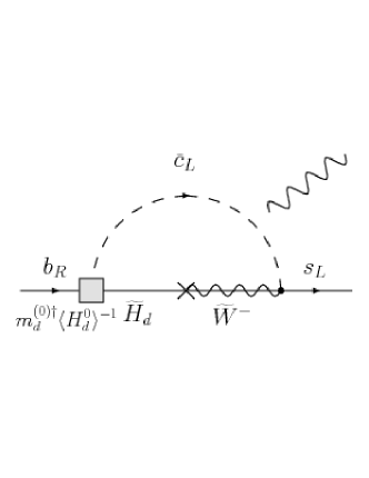
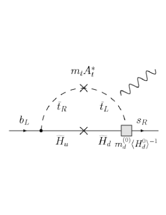
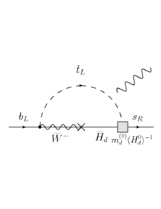
Figure 9: BLO corrections to $C_{7}$ ($C_{8}$) and $C_{7}^{\prime}$ ($C_{8}^{\prime}$) arising from chargino exchange, the photon (gluon) line is attached in every possible manner.

The effect of BLO corrections in the limit of MFV are well known [11, 14]. In GFM models, however, it is possible that additional sources of flavour violation in both the up and down squark sectors can significantly alter the MFV result.

Contributions from flavour violation in the up squark sector enter at LO and are therefore rather large. As we are chiefly concerned with flavour violation in the down squark sector, the only relevant source of flavour violation in the up squark sector is the insertion $\delta_{LL}^{u}$, which is related, by ${\rm SU}\left(2\right)$ symmetry, to $\delta_{LL}^{d}$ (22). Flavour violation in the down squark sector, on the other hand, only enters via BLO effects induced by the off–diagonal elements of $m_{d}^{(0)}$.

The contributions that arise due to LL insertions have the form

$$\left(\delta^{\chi^{-}}C_{7,8}\right)^{\rm LL}=\frac{K_{cs}^{\ast}}{K_{ts}^{\ast}}\sum_{a=1}^{2}\bigg{\{}\frac{m_{W}^{2}}{m_{\chi^{-}_{a}}^{2}}y_{a}\bigg{[}V_{a1}^{\ast}V_{a1}I_{1}^{[7,8]}\left(y_{\widetilde{d}}^{a}\right)$$

$$-\frac{m_{\chi^{-}_{a}}}{m_{W}}\frac{U_{a2}^{\ast}V_{a1}}{\sqrt{2}\cos\beta\left(1+\epsilon_{3}\tan\beta\right)}I_{2}^{[7,8]}\left(y_{\widetilde{d}}^{a}\right)\bigg{]}\delta_{LL}^{u}$$

$$+\frac{K_{cs}}{K_{tb}}\frac{m_{W}}{m_{\chi^{-}_{a}}}\frac{U_{a2}^{\ast}V_{a1}\epsilon_{LL}x_{\widetilde{d}}\tan\beta}{\sqrt{2}\cos\beta\left(1+\epsilon_{s}\tan\beta\right)\left(1+\epsilon_{3}\tan\beta\right)}\left(H_{2}^{[7,8]}\left(y_{\widetilde{d}}^{a}\right)+\lambda^{[7,8]}\right)\delta_{LL}^{d}\bigg{\}}.$$ (102)

Once again the loop functions $H_{i}^{[7,8]}$ and $I_{i}^{[7,8]}$ can be found in appendix A.2, the ratio $y_{\widetilde{d}}^{a}$ is given by

$$y_{\widetilde{d}}^{a}=\frac{m_{\widetilde{q}}^{2}}{m_{\chi^{-}_{a}}^{2}}.$$ (103)

The dominant contribution at LO for large $\tan\beta$ arises from the second term in square brackets in (102) that is enhanced by factors of $m_{\chi^{-}_{a}}/m_{W}$ and $1/\cos\beta$. This term, for $\mu>0$, has the same sign as the gluino contribution (98) and acts to enhance the contributions due to flavour violation in the LL sector. The BLO corrections to the Wilson coefficient are reflected by a factor of $\left(1+\epsilon_{3}\tan\beta\right)$ that appears in the denominator of the second term in square brackets in (102), and the term that appears in the second line of (102), proportional to $\delta_{LL}^{d}$. Both of these BLO corrections for $\mu>0$ act to decrease the LO contribution. For $\mu<0$, on the other hand, both corrections act to increase the Wilson coefficient relative to the LO result.

The LR insertions also contribute to the Wilson coefficient

$$\left(\delta^{\chi^{-}}C_{7,8}\right)^{\rm LR}= -\frac{K_{cs}K_{cs}^{\ast}}{K_{tb}K_{ts}^{\ast}}\sum_{a=1}^{2}\frac{m_{W}}{\sqrt{2}m_{\chi^{-}_{a}}\cos\beta}V_{a1}U_{a2}^{\ast}\frac{m_{\widetilde{g}}}{m_{b}}\frac{\epsilon_{RL}x_{\widetilde{d}}}{\left(1+\epsilon_{s}\tan\beta\right)}$$

$$\times \left(H_{2}^{[7,8]}\left(y_{\widetilde{d}}^{a}\right)+\lambda^{[7,8]}\right)\delta_{LR}^{d}.$$ (104)

In this case, GFM contributions only enter via BLO effects induced by the off–diagonal elements of the bare mass matrix. For $\mu>0$ and large $\tan\beta$, the contribution (104) has the opposite sign to the gluino contribution (99) and large cancellations are possible, which contribute significantly to the focusing effect pointed out in [15].

Before proceeding with the results relevant to the primed sector we should note that once again, the contributions to $C_{7,8}$ arising from RL and RR insertions are suppressed by factors of $m_{s}$.

In a similar manner to the corrections that arise from gluino exchange, the only dominant contributions to the primed coefficients arise from RL and RR insertions. The contribution arising from RL insertions is given by

$$\left(\delta^{\chi^{-}}C_{7,8}^{\prime}\right)^{\rm RL}= \sum_{a=1}^{2}\frac{K_{tb}^{\ast}}{K_{ts}^{\ast}m_{\chi^{-}_{a}}}\Bigg{[}\frac{m_{t}^{2}A_{t}}{2m_{\chi^{-}_{a}}^{2}}V^{\ast}_{a2}U_{a2}\tan\beta I_{2}^{[7,8]}\left(y_{\widetilde{d}}^{a}\right)$$

$$-\frac{m_{W}}{\sqrt{2}\cos\beta}V^{\ast}_{a1}U_{a2}\left(H_{2}^{[7,8]}\left(y_{\widetilde{d}}^{a}\right)+\lambda^{[7,8]}\right)\Bigg{]}\frac{m_{\widetilde{g}}}{m_{b}}\frac{\epsilon_{RL}x_{\widetilde{d}}}{\left(1+\epsilon_{3}\tan\beta\right)}\delta_{RL}^{d},$$ (105)

and the contribution arising from RR insertions is

$$\left(\delta^{\chi^{-}}C_{7,8}^{\prime}\right)^{\rm RR}= -\sum_{a=1}^{2}\frac{K_{tb}^{\ast}}{K_{ts}^{\ast}m_{\chi^{-}_{a}}}\Bigg{[}\frac{m_{t}^{2}A_{t}}{2m_{\chi^{-}_{a}}^{2}}V^{\ast}_{a2}U_{a2}\tan\beta I_{2}^{[7,8]}\left(y_{\widetilde{d}}^{a}\right)$$

$$-\frac{m_{W}}{\sqrt{2}\cos\beta}V^{\ast}_{a1}U_{a2}\left(H_{2}^{[7,8]}\left(y_{\widetilde{d}}^{a}\right)+\lambda^{[7,8]}\right)\Bigg{]}\frac{\epsilon_{RR}x_{\widetilde{d}}\tan\beta}{\left(1+\epsilon_{3}\tan\beta\right)^{2}}\delta_{RR}^{d}.$$ (106)

LO contributions to both coefficients arising from either MFV or non–zero $\delta_{LL}^{u}$ are suppressed by factors of $m_{s}/m_{b}$ and are therefore rather small. At large $\tan\beta$, therefore, the BLO effects dominate the behaviour of the chargino contributions to the primed operators. We should also note that in a similar manner to the case of the LR insertion both corrections (for $\mu>0$) have the opposite sign to the gluino contributions (100)–(101).

In the GFM scenario, neutralino contributions also play a rôle. They can become especially important when, for example, the gluino and chargino contributions partially cancel [44]. However, as the neutralino couplings (161)–(162) are rather complicated, we shall refrain from presenting complete analytic expressions for the coefficients in the MIA. The overall effect of including BLO corrections is to modify the Wilson coefficient in a similar manner to the gluino contributions (99)–(101). As an example, the contribution arising from LR insertions to $C_{7,8}$ due to bino exchange becomes

$$\left(\delta^{\tilde{B}}C_{7}\right)^{\rm LR}=\frac{m_{W}^{2}\tan^{2}\theta_{W}}{9K_{ts}^{\ast}K_{tb}m_{b}M_{1}}\frac{z_{\tilde{d}}I_{4}^{[7,8]}\left(z_{\tilde{d}}\right)}{\left(1+\epsilon_{s}\tan\beta\right)}\delta_{LR}^{d}.$$ (107)

The loop function $I_{4}^{[7,8]}$ can be found in appendix A.2 whilst its argument is given by $z_{\tilde{d}}=m_{\widetilde{q}}^{2}/M_{1}^{2}$. The contributions induced by neutral gaugino–higgsino mixing, on the other, hand are more complicated due to the appearance of the bare quark mass matrix in the couplings (161)–(162).

Finally, let us consider the effect of evolving these coefficients from the SUSY matching scale $\mu_{SUSY}$ to the electroweak scale $\mu_{W}$. Considering only the mixing between $\mathcal{O}_{7}$ and $\mathcal{O}_{8}$ we have the LO relation [47]

$$\delta C_{7}\left(\mu_{W}\right)=\eta^{\frac{16}{21}}\delta C_{7}\left(\mu_{SUSY}\right)+\frac{8}{3}\left(\eta^{\frac{2}{3}}-\eta^{\frac{16}{21}}\right)\delta C_{8}\left(\mu_{SUSY}\right).$$ (108)

The factors of $\eta$ in the above expression reflect the resummation of leading logarithms and are given by

$$\eta=\frac{\alpha_{s}\left(\mu_{SUSY}\right)}{\alpha_{s}\left(\mu_{W}\right)},$$ (109)

where $\alpha_{s}\left(\mu_{SUSY}\right)$ and $\alpha_{s}\left(\mu_{W}\right)$ should be evaluated with the QCD $\beta$ function relevant for six active flavours. If we retain only the first logarithm that appears when expanding the factors $\eta$ we have

$$\delta C_{7}\left(\mu_{W}\right)=\delta C_{7}\left(\mu_{SUSY}\right)-\frac{4}{3\pi}\alpha_{s}\left(\mu_{W}\right)\left[\delta C_{7}\left(\mu_{SUSY}\right)-\frac{1}{3}\delta C_{8}\left(\mu_{SUSY}\right)\right]\log\frac{\mu_{SUSY}^{2}}{\mu_{W}^{2}}.$$ (110)

From the above expression, it is apparent that the evolution of the coefficients from $\mu_{SUSY}$ to $\mu_{W}$ acts to reduce the overall SUSY contribution. In addition mixing with the coefficient $C_{8}$ can also play a rôle. If $\delta C_{8}$ has the opposite sign compared to $\delta C_{7}$, for example, further reductions are possible.

Finally, let us provide a recipe for implementing BLO corrections into existing LO gluino matching conditions calculated in the MIA [45, 46]. When performing LO calculations, one ignores the corrections to the bare mass matrix, discussed in section 2.1, and the $F$–terms are therefore assumed to be flavour diagonal. Once one proceeds beyond the LO however, this assumption no longer holds and additional off–diagonal elements in the squark mass matrix appear, that are attributable to the factors of $m_{d}^{(0)}$ that appear in (16). In the LR sector, in particular, the off–diagonal elements of the bare mass matrix are enhanced by a factor of $\tan\beta$. The effect of these BLO corrections can be included in existing LO expressions by making the following substitutions

$$\left(\delta_{LR}^{d}\right)_{ij} \to\left(\delta_{LR}^{d}\right)_{ij}-\frac{\mu\tan\beta\left(m_{d}^{(0)}{}^{{\dagger}}\right)_{ij}}{\sqrt{\left(m_{d,LL}^{2}\right)_{ii}\left(m^{2}_{d,RR}\right)_{jj}}},$$ (111)

$$\left(\delta_{RL}^{d}\right)_{ij} \to\left(\delta_{RL}^{d}\right)_{ij}-\frac{\mu\tan\beta\left(m_{d}^{(0)}\right)_{ij}}{\sqrt{\left(m_{d,RR}^{2}\right)_{ii}\left(m^{2}_{d,LL}\right)_{jj}}}.$$ (112)

Similar substitutions exist for the insertions $\delta_{LL}^{d}$ and $\delta_{RR}^{d}$, however the effects are typically proportional to $\mathcal{O}(m_{b}^{2}/m_{SUSY}^{2})$ and may therefore be safely omitted. In each of the substitutions given above, the off–diagonal elements of the bare mass matrix are enhanced by a factor of $\tan\beta$ and can therefore play a rather large rôle. One should also note that the factor of the down quark mass, that appears in flavour–diagonal LR mixings, should also be replaced by the appropriate element of $m_{d}^{(0)}$. Following this recipe, it is relatively easy to modify the LO calculation presented in, for example, [45] and obtain results in agreement with those presented above. We should note that, provided one calculates $m_{d}^{(0)}$ to a similar precision, the substitutions can be used to all orders in the MIA. One may also use these substitutions in LO expressions for the chargino and neutralino matching conditions, however here one must also take into account the factors of the bare mass matrix that appear in the chargino and neutralino vertices. Finally, let us emphasise that the substitutions (111)–(112) do not amount to a redefinition of the $\delta$’s given in (20)–(21) but merely represent the form of the BLO corrections to LO expressions.

4.3 Full Calculation

With our results derived in the MIA in mind let us now outline the steps required to implement BLO corrections in the general framework outlined in section 2 where the squark mass matrices are diagonalised numerically. After performing the iterative procedure described in subsection 2.4 one may obtain the BLO charged Higgs and SM contributions by using the matching conditions presented in [37, 36, 38], to account for the NLO gluon contribution, and using the corrected vertices presented in section 2 to evaluate the LO matching conditions. As discussed in subsection 3.2 the corrections to the SM contributions tend to be rather small and can generally be ignored. The effect of the neutral Higgs contribution can also be included by using the matching conditions presented in [3, 14].

Turning to the supersymmetric contributions, BLO corrections can be incorporated by using the supersymmetric vertices detailed in section 2.3 and appendix C in the LO matching conditions given in [38, 16]. It should be noted that one should use the unitary matrices $\Gamma_{d,u}$ that are obtained at the end of the iterative procedure described in subsection 2.4 when evaluating these contributions. One may also, with care, include the additional NLO effects that appear if the gluino decouples by using the matching conditions presented in [38]. Once one has evaluated all the supersymmetric corrections they may be evolved from the SUSY matching scale to the electroweak matching scale using the NLO six flavour anomalous dimension matrix presented in [47].

With the supersymmetric and electroweak contributions evaluated at the scale $\mu_{W}$ it is finally possible to calculate the branching ratio for $\bar{B}\to X_{s}\gamma$ according to [30]. Let us note that this recipe is quite general and may be applied to any other process providing the relevant matching conditions and anomalous dimension matrices are available.

In summary, in this section we have included all the relevant corrections that appear beyond the LO in the MIA. In the electroweak sector, we have seen that the additional GFM contributions to the charged and neutral Higgs vertices can lead to potentially large modifications to the MFV results depending on the sign of the insertion at hand. The interplay and cancellations between the various supersymmetric contributions, has also been shown to be significant once one proceeds BLO [15] and leads to a focusing effect in the phenomenologically interesting region $\mu>0$ and $A_{t}<0$. For the insertions $\delta_{LR}^{d}$, $\delta_{RL}^{d}$ and $\delta_{RR}^{d}$, in particular, large cancellations can arise between the gluino and chargino contributions to the decay. For the insertion $\delta_{LL}^{d}$ on the other hand, the cancellations play a more minor role, as a LO correction to the chargino correction already exists (arising from the insertion $\delta_{LL}^{u}$) and tends to reduce the effect of BLO corrections. Finally we have seen that the RG evolution of these corrections can lead to further reductions to the supersymmetric contributions to the decay.

5 $\bar{B}_{s}\to\mu^{+}\mu^{-}$ Beyond the LO

As B–factories do not run at the energy required to produce large quantities of $B_{s}$ mesons, the best experimental constraint on the rare decay $\bar{B}_{s}\to\mu^{+}\mu^{-}$ is provided by collider experiments. The current 95% confidence limits provided by the CDF [48] and DØ [49] experiments at the Tevatron are

$${\rm BR}\left(\bar{B}_{s}\to\mu^{+}\mu^{-}\right)_{\rm CDF}<2.0\times 10^{-7},$$ (113)

$${\rm BR}\left(\bar{B}_{s}\to\mu^{+}\mu^{-}\right)_{\rm D{\O}}<3.8\times 10^{-7}.$$ (114)

CDF and DØ intend to further probe regions of up to $\mathcal{O}\left(10^{-8}\right)$. At the LHC, on the other hand, branching ratios of up to $\mathcal{O}\left(10^{-9}\right)$ are easily obtainable after a few years of running at ATLAS, CMS and LHCb [52].

Theoretically, the decay $\bar{B}_{s}\to\mu^{+}\mu^{-}$ provides one of the cleanest FCNC $\Delta F=1$ decay channels. It is described by the effective Hamiltonian [23]

$$\mathcal{H}_{eff}=-\frac{G_{F}\alpha}{\sqrt{2}\pi}K^{\rm eff}_{ts}{}^{*}K^{\rm eff}_{tb}\sum_{i}\left[C_{i}(\mu)\mathcal{O}_{i}(\mu)+C_{i}^{\prime}(\mu)\mathcal{O}_{i}^{\prime}(\mu)\right]$$ (115)

where the operators $\mathcal{O}_{i}$ are given by

$$\mathcal{O}_{10} =\left(\bar{s}_{\alpha}\gamma^{\mu}P_{L}b_{\alpha}\right)\left(\bar{l}\gamma_{\mu}\gamma_{5}l\right), \mathcal{O}_{10}^{\prime} =\left(\bar{s}_{\alpha}\gamma^{\mu}P_{R}b_{\alpha}\right)\left(\bar{l}\gamma_{\mu}\gamma_{5}l\right),$$

$$\mathcal{O}_{S} =m_{b}\left(\bar{s}_{\alpha}P_{R}b_{\alpha}\right)\left(\bar{l}l\right), \mathcal{O}_{S}^{\prime} =m_{s}\left(\bar{s}_{\alpha}P_{L}b_{\alpha}\right)\left(\bar{l}l\right),$$

$$\mathcal{O}_{P} =m_{b}\left(\bar{s}_{\alpha}P_{R}b_{\alpha}\right)\left(\bar{l}\gamma_{5}l\right), \mathcal{O}_{P}^{\prime} =m_{s}\left(\bar{s}_{\alpha}P_{L}b_{\alpha}\right)\left(\bar{l}\gamma_{5}l\right).$$ (116)

As the anomalous dimensions of all three operators are zero, the RG running is trivial and the overall branching ratio for the process $l=\mu$ is given by

$${\rm BR}\left(\bar{B}_{s}\to\mu^{+}\mu^{-}\right)= \frac{G_{F}^{2}\alpha^{2}m_{B_{s}}^{2}f_{B_{s}}^{2}\tau_{B_{s}}}{64\pi^{3}}\lvert K^{\rm eff}_{ts}{}^{\ast}K^{\rm eff}_{tb}\rvert^{2}\sqrt{1-4\hat{m}_{\mu}^{2}}$$

$$\times\left[\left(1-4\hat{m}_{\mu}^{2}\right)\lvert F_{S}\rvert^{2}+\lvert F_{P}+2\hat{m}_{\mu}^{2}F_{10}\rvert^{2}\right],$$ (117)

where $\hat{m}_{\mu}=m_{\mu}/m_{B_{s}}$ and the dimensionless quantities $F_{i}$ are given by

$$F_{S,P} =m_{B_{s}}\left[\frac{C_{S,P}m_{b}-C_{S,P}^{\prime}m_{s}}{m_{b}+m_{s}}\right], F_{10}=C_{10}-C_{10}^{\prime}.$$

It should be noted from the above expression that the Wilson coefficient of the operator $\mathcal{O}_{10}$ is helicity suppressed by a factor of $\hat{m}_{\mu}^{2}$ as the $B_{s}$ meson has spin zero. The SM contributions are only proportional to $\mathcal{O}_{10}$ as the Higgs mediated contributions to $\mathcal{O}_{S,P}$ can be safely neglected. The SM contributions to $C_{10}$ have been evaluated to NLO [53] resulting in the branching ratio [54]

$${\rm BR}\left(\bar{B}_{s}\to\mu^{+}\mu^{-}\right)_{\rm SM}=\left(3.46\pm 1.5\right)\times 10^{-9}.$$ (118)

The large uncertainty is mainly attributable to the hadronic matrix element $f_{B_{s}}$ that can be determined from either lattice or QCD sum rule calculations. A representative value for $f_{B_{s}}$ is

$$f_{B_{s}}=\left(230\pm 30\right)\,\mbox{MeV}.$$ (119)

In scenarios beyond the SM, particularly SUSY with large $\tan\beta$, the contributions to $C_{S}$ and $C_{P}$ arising from neutral Higgs penguins can become large and dominate the underlying behaviour of the branching ratio. Studies in the MSSM have focussed on both MFV [58, 22, 60] and GFM scenarios [61, 62, 17] where the corrections induced by the corrected neutral Higgs vertex (66)–(67) lead the branching ratio for the decay to vary as $\tan^{6}\beta$ (for a review see [24]). At large $\tan\beta$ it is therefore quite possible for ${\rm BR}\left(\bar{B}_{s}\to\mu^{+}\mu^{-}\right)$ to be enhanced by a few a orders of magnitude compared to the SM value, providing an ideal signal for physics beyond the SM. The aim of this section is to present analytic expressions for the contributions to $C_{S}$ and $C_{P}$ in the MIA that include the BLO effects discussed in section 2. We also discuss briefly the effect BLO contributions have on the subdominant contributions that arise from box diagrams mediated by neutralinos and charginos. Finally we discuss the application of the recipe given at the end of the previous section to $\bar{B}_{s}\to\mu^{+}\mu^{-}$.

5.1 BLO Corrections to Electroweak Contributions in the MIA

As above for $\bar{B}\to X_{s}\gamma$, here we will present MIA calculations for the contributions that arise due to the effective vertices presented in section 2.2.

Corrections to the effective $Z$ vertex 50 lead to contributions to $C_{10}$ proportional to $\delta_{LR}^{d}$

$$\left(\delta^{Z}C_{10}\right)^{\rm GFM}= \frac{1}{3K_{tb}K_{ts}^{*}}\frac{\alpha_{s}}{\alpha}\frac{\mu m_{b}}{m_{\widetilde{g}}^{2}}\frac{\tan\beta}{\left(1+\epsilon_{s}\tan\beta\right)\left(1+\epsilon_{3}\tan\beta\right)}f_{Z}\left(x_{\widetilde{d}}\right)\;\delta_{LR}^{d}$$ (120)

whilst there is a similar contribution proportional to $\delta_{RL}^{d}$ to $C_{10}^{\prime}$. Terms proportional to $\delta_{LL}^{d}$ may be generated at third order in the MIA, which undergo BLO corrections from terms that appear when using the bare mass matrix (45). As stated in the previous section however, $C_{10}$ and $C_{10}^{\prime}$ are both helicity suppressed by factors of $m_{\mu}^{2}$ and their contribution to the overall branching ratio is therefore typically limited to the low $\tan\beta$ regime.

The charged Higgs contributions to $C_{10}$ and $C_{10}^{\prime}$ arise from $Z$ penguins and box diagrams. The contribution to $C_{10}$ is suppressed by a factor of $\cot^{2}\beta$ and, whilst the contribution to $C_{10}^{\prime}$ is enhanced by a factor of $\tan^{2}\beta$, it is suppressed by a factor of $m_{s}$. Including BLO effects can alleviate these suppression factors. However, as the Wilson coefficients are suppressed by a factor of $m_{\mu}^{2}$ the overall effect is rather small.

The LO contributions to $C_{S,P}$ induced by neutral Higgs penguins and box diagrams have been calculated in [22]. For completeness we present them here

$$\delta^{H^{-}}C_{S,P}^{(0)} =\pm\frac{m_{\mu}\tan^{2}\beta}{4m_{W}^{2}\sin^{2}\theta_{W}}\frac{y\log y}{1-y}, \delta^{H^{-}}C_{S,P}^{(0)\;\prime} =\pm\left(\delta^{H^{-}}C_{S,P}^{(0)}\right)$$ (121)

where $y=m_{t}^{2}/m_{H^{+}}^{2}$.

BLO effects can be included by using the couplings presented in subsection 3.2 when calculating the matching conditions. The largest correction induced by using these couplings is attributable to the factor of $\left(1+\epsilon_{3}\tan\beta\right)$ that accompanies the right handed coupling of the charged Higgs. This factor typically acts to reduce the charged Higgs contribution relative to the LO prediction. The GFM corrections to the vertex can act to replace the factors of $K_{ts}^{\ast}K_{tb}$ that characterise flavour change in the MFV contribution with the flavour violating insertions (20)–(21).

The contributions that arise due to the corrected neutral Higgs vertex proceed via the penguin diagram shown in Fig. 10.

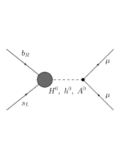
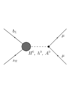
Figure 10: The neutral Higgs penguin contributions to $C_{S,P}$ (on the left) and $C_{S,P}^{\prime}$ (on the right).

Using (66) it is relatively easy to obtain the dominant contribution arising from chargino exchange in the limit of MFV [58, 60]

$$\left(\delta^{H^{0}}C_{S,P}\right)^{\rm MFV}= \pm\frac{m_{\mu}m_{t}^{2}A_{t}\tan^{3}\beta}{4m_{W}^{2}m_{A}^{2}\mu\sin^{2}\theta_{W}}\frac{H_{2}\left(y_{\widetilde{u}_{R}},y_{\widetilde{u}_{L}}\right)}{\left(1+\epsilon_{3}\tan\beta\right)\left(1+\epsilon_{s}\tan\beta\right)}.$$ (122)

$m_{A}$ denotes the mass of the pseudoscalar Higgs, whilst we decompose the MFV and GFM contributions in a similar manner to (65). The most striking aspect of this contribution stems from the factor of $\tan^{3}\beta$ that appears in the numerator of (122) coupled with a relatively weak dependence on the underlying SUSY mass scale. It is therefore possible in SUSY models with large $\tan\beta$ that large contributions to $C_{S,P}$ can occur even if the sparticle masses are $\mathcal{O}\left(1\,\mbox{TeV}\right)$. (Provided, of course, that the Higgs sector does not decouple, too.) The BLO contributions in (122) are contained in the factors of $\left(1+\epsilon_{3}\tan\beta\right)$ and $\left(1+\epsilon_{s}\tan\beta\right)$ that appear in the denominator. In the limit of degenerate sparticle masses, for $\mu>0$, these corrections tend to reduce the neutral Higgs contribution to $C_{S,P}$ compared with the LO limit $\epsilon_{Y},~{}\epsilon_{s}\to 0$.

The GFM corrections to the effective neutral Higgs vertex (67) contribute to $C_{S,P}$ [17]

$$\left(\delta^{H^{0}}C_{S,P}\right)^{\rm GFM}= \pm\frac{4\alpha_{s}}{3\alpha}\frac{\mu m_{\mu}}{m_{A}^{2}}\frac{\tan^{3}\beta}{K_{tb}K_{ts}^{\ast}}\Bigg{[}\frac{\epsilon_{RL}}{\left(1+\epsilon_{s}\tan\beta\right)}\frac{x_{\widetilde{d}_{RL}}}{m_{b}}H_{2}(x_{\widetilde{d}_{R}},x_{\widetilde{d}_{L}})\delta_{LR}^{d}$$

$$+ \frac{1}{\left(1+\epsilon_{s}\tan\beta\right)\left(1+\epsilon_{3}\tan\beta\right)}\frac{x_{\widetilde{d}_{L}}}{m_{\widetilde{g}}}H_{3}(x_{\widetilde{d}_{R}},x_{\widetilde{d}_{L}},x_{\widetilde{d}_{L}})\delta_{LL}^{d}\Bigg{]},$$ (123)

and the primed coefficients

$$\left(\delta^{H^{0}}C_{S,P}^{\prime}\right)^{\rm GFM}= \frac{4\alpha_{s}}{3\alpha}\frac{\mu m_{\mu}}{m_{A}^{2}}\frac{\tan^{3}\beta}{K_{tb}K_{ts}^{\ast}}\Bigg{[}\frac{\left(\epsilon_{RL}+\frac{m_{\widetilde{g}}}{\mu}\epsilon_{Y}Y_{t}^{2}\right)}{\left(1+\epsilon_{3}\tan\beta\right)}\frac{x_{\widetilde{d}_{RL}}}{m_{s}}H_{2}(x_{\widetilde{d}_{L}},x_{\widetilde{d}_{R}})\delta_{RL}^{d}$$

$$+\frac{1}{\left(1+\epsilon_{3}\tan\beta\right)^{2}}\frac{x_{\widetilde{d}_{R}}}{m_{\widetilde{g}}}\frac{m_{b}}{m_{s}}H_{3}(x_{\widetilde{d}_{L}},x_{\widetilde{d}_{R}},x_{\widetilde{d}_{R}})\delta_{RR}^{d}\Bigg{]}.$$ (124)

The contributions arising from the insertions $\delta_{LL}^{d}$ and $\delta_{RR}^{d}$ are modified in a similar manner to the MFV contribution (122) and for $\mu>0$ undergo the familiar reduction once BLO effects are taken into account. It should be noted that once one proceeds beyond the approximation of setting electroweak couplings to zero, and uses the substitutions gathered in subsection 3.3 an additional contribution, proportional to the insertion, $\delta_{LL}^{d}$ arises

$$\left(\delta^{H^{0}}C_{S,P}\right)^{\rm EW}=\mp\sum_{a=1}^{2}\frac{m_{\mu}V_{a1}^{\ast}m_{\chi^{-}_{a}}U_{a2}}{2\sqrt{2}m_{W}m_{A}^{2}}\frac{\tan^{3}\beta}{K_{tb}K_{ts}^{\ast}\sin\beta\sin^{2}\theta_{W}}y_{\widetilde{d}_{L}}^{a}H_{2}\left(y_{\widetilde{u}_{L}}^{a},y_{\widetilde{u}_{L}}^{a}\right)\delta_{LL}^{d}$$ (125)

This LO correction tends to interfere destructively with the dominant gluino contribution given in (123) and is typically the largest contribution attributable to the insertion $\delta_{LL}^{d}$ once one proceeds beyond the approximation described in section 3.

Turning to the insertions $\delta_{LR}^{d}$ and $\delta_{RL}^{d}$, their appearance is a strictly BLO effect and can lead to large deviations from LO results where the contributions arising from the insertions accidentally cancel as we have shown in [17].

5.2 BLO Corrections to SUSY Contributions

As the gluino does not couple to the leptonic sector the supersymmetric contributions to $\bar{B}_{s}\to\mu^{+}\mu^{-}$ take place via the box diagrams mediated by chargino and neutralino exchange shown in Fig. 11.

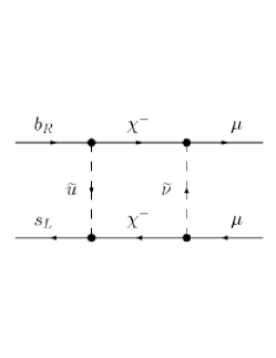
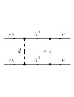
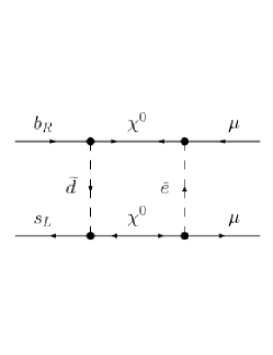
Figure 11: The contributions to $\bar{B}_{s}\to\mu^{+}\mu^{-}$ arising from box diagrams mediated by charginos and neutralinos.

Including BLO effects when calculating these contributions introduces a dependence on the bare mass matrix, through the vertices (36)–(37) and (161)–(162). Sources of flavour violation can therefore enter through either the chargino or the neutralino contributions. However these contributions tend to scale as $\tan^{2}\beta$ and, coupled with the underlying dependence on $1/M_{SUSY}^{2}$, rather than $1/m_{A}^{2}$, are rather small when compared to the effects induced by the neutral Higgs penguins discussed in the previous subsection.

5.3 Full Calculation

During our numerical analysis we shall follow the recipe described in subsection 4.3 and use the expressions gathered in appendix D to evaluate the corrections to the various effective vertices. We therefore include higher order terms in the MIA as well as any (subdominant) ${\rm SU}(2)_{L}\times{\rm U}(1)_{Y}$ breaking effects. Concerning the SM and charged Higgs contributions to the decay we use the matching conditions gathered in [63] to evaluate the NLO gluon contribution. The contributions that arise from SUSY boxes are given in [59, 22].

In conclusion, in this section we have discussed how the BLO effects discussed in section 2 alter LO contributions to $\bar{B}_{s}\to\mu^{+}\mu^{-}$. In the electroweak sector, these corrections typically manifest themselves as factors of either $\left(1+\epsilon_{3}\tan\beta\right)$ or $\left(1+\epsilon_{s}\tan\beta\right)$ that act to reduce both MFV and GFM contributions to the decay. In addition, we have seen that new flavour structures, absent at LO, can appear once BLO effects are taken into account, leading to potentially large deviations from LO calculations.

6 $\bar{B}_{s}-B_{s}$ Mixing Beyond the LO

The final process that we will consider concerns mixing in the $B_{s}$ meson system. In a similar manner to the neutral kaon and $B_{d}$ systems mixing can occur between the $B_{s}$ and $\bar{B}_{s}$ mesons via $\Delta F=2$ loop diagrams. In contrast to the neutral kaon and $B_{d}$ systems, however, the mass difference $\Delta M_{B_{s}}$ between the physical states formed from the two mesons has so far remained unobserved. The best bound provided by experiment is currently [27]

$$\Delta M_{B_{s}}^{\rm exp}>14.5\,\mbox{ps}^{-1}.$$ (126)

In future, the experiments at the Tevatron intend to increase this limit by 20–30% [64] whilst even after a year of low luminosity running ATLAS, CMS and LHCb intend to place limits of $30{\rm ps}^{-1}$, $26{\rm ps}^{-1}$ and $48{\rm ps}^{-1}$ [52] respectively on $\Delta M_{B_{s}}$. Comparing these limits with the NLO Standard Model prediction [65, 66]

$$\Delta M_{B_{s}}^{\rm SM}=\left(18.0\pm 3.7\right)\,\mbox{ps}^{-1},$$ (127)

it can be seen that the full range of values allowed by the SM can be probed in a relatively short time after data taking has commenced at the LHC.

The effective Hamiltonian that most generally describes $\bar{B}_{s}-B_{s}$ mixing effects is given by [67, 68]

$$\mathcal{H}_{eff}=\frac{G_{F}^{2}}{16\pi^{2}}m_{W}^{2}\left(K^{\rm eff}_{tb}{}^{*}K^{\rm eff}_{ts}\right)^{2}\sum_{i}C_{i}\left(\mu\right)\mathcal{O}_{i}\left(\mu\right).$$ (128)

In the SM the only non-negligible contribution is proportional to the operator

$$\mathcal{O}^{VLL} =(\bar{b}^{\alpha}\gamma_{\mu}P_{L}s^{\alpha})(\bar{b}^{\beta}\gamma^{\mu}P_{L}s^{\beta}).$$ (129)

However, in the presence of any source of new physics it is possible to induce additional contributions to the operators

$$\mathcal{O}^{LR}_{1} =(\bar{b}^{\alpha}\gamma_{\mu}P_{L}s^{\alpha})(\bar{b}^{\beta}\gamma^{\mu}P_{R}s^{\beta}), \mathcal{O}^{LR}_{2} =(\bar{b}^{\alpha}P_{L}s^{\alpha})(\bar{b}^{\beta}P_{R}s^{\beta}),$$ (130)

$$\mathcal{O}^{SLL}_{1} =(\bar{b}^{\alpha}P_{L}s^{\alpha})(\bar{b}^{\beta}P_{L}s^{\beta}), \mathcal{O}^{SLL}_{2} =(\bar{b}^{\alpha}\sigma_{\mu\nu}P_{L}s^{\alpha})(\bar{b}^{\beta}\sigma^{\mu\nu}P_{L}s^{\beta}),$$ (131)

as well as the parity flipped operators $\mathcal{O}^{VRR}$ and $\mathcal{O}^{SRR}_{i}$ that can be obtained by substituting $P_{L}$ with $P_{R}$ in (129) and (131). The mass difference $\Delta M_{B_{s}}$ may then be evaluated by taking the matrix element

$$\Delta M_{B_{s}}=2\lvert\langle\bar{B}^{0}_{s}\lvert\mathcal{H}_{eff}\rvert B^{0}_{s}\rangle\rvert,$$ (132)

where $\langle\bar{B}^{0}_{s}\lvert\mathcal{H}_{eff}\rvert B^{0}_{s}\rangle$ is given by

$$\langle\bar{B}^{0}_{s}\lvert\mathcal{H}_{eff}\rvert B^{0}_{s}\rangle= \frac{G_{F}^{2}}{48\pi^{2}}m_{W}^{2}m_{B_{s}}f_{B_{s}}\left(K^{\rm eff}_{tb}{}^{\ast}K^{\rm eff}_{ts}\right)^{2}\sum_{i}P_{i}C_{i}\left(\mu_{W}\right),$$ (133)

$m_{B_{s}}$ denotes the mass of the $B_{s}$ meson, whilst $f_{B_{s}}$ is given in (119). The coefficients $P_{i}$ contain the effects due to RG running between $\mu_{t}$ and $\mu_{b}$ as well as the relevant hadronic matrix element for the operator in question. Using the $\overline{{\rm MS}}$ lattice calculation [69] the coefficients $P_{i}$ have the form

$$P^{VLL}_{1}= 0.73, P^{LR}_{1}= -1.97, P^{LR}_{2}= 2.50, P^{SLL}_{1}= -1.02, P^{SLL}_{2}= -1.97.$$ (134)

where we have taken $\mu_{b}=4.25\,\mbox{GeV}$ and $\mu_{W}=m_{t}(m_{t})$. The coefficients $P^{VRR}_{1}$, etc., may be obtained by simply exchanging $L$ and $R$. One interesting aspect of (134) is that QCD effects act to enhance the contributions arising from the scalar operators relative to the SM operator $C^{VLL}$.

The new physics contributions to neutral meson mixing have been discussed extensively in the literature. The NLO charged Higgs contributions to $C^{VLL}$, for instance, have been known for some time now [70]. Turning to the MSSM, the NLO matching conditions have, in a similar manner to the decay $\bar{B}\to X_{s}\gamma$, only been derived for some special cases in the MFV limit [71]. Most analyses have therefore focussed on using LO matching conditions. For example, in [72] the LO gluino matching conditions, relevant for mixing in the kaon system, were used alongside the NLO anomalous dimension matrix and lattice matrix elements to place limits on the insertions governing non–minimal flavour violation between down and strange squarks. This analysis has since been extended to the $B_{d}$ [73] and $B_{s}$ [74] meson systems. In the $\bar{B}_{s}-B_{s}$ mixing system, in particular, large contributions to $\Delta M_{B_{s}}$ of up to $120\,\mbox{ps}^{-1}$ have been found to arise. In the large $\tan\beta$ regime another possibility for large contributions arises from the inclusion of the effects induced by the neutral Higgs penguin. Although strictly speaking an NLO contribution the corrections arising from flavour violation mediated by two neutral Higgs penguins have been shown to vary as $\tan^{4}\beta$. Such corrections have been analysed in the context of MFV [75, 61, 76, 60, 14] and GFM [75, 61, 62, 17] and can similarly induce rather large corrections to $\Delta M_{B_{s}}$.

The aim of this section is to discuss how the inclusion of BLO corrections affect the electroweak and supersymmetric contributions to the Wilson coefficients associated with the operators (129)–(131). In particular, we shall discuss, in detail, the contributions that arise from double Higgs penguins in the GFM scenario and the dominant BLO corrections to the existing LO gluino matching conditions. When presenting our analytic expressions we shall use the MIA and follow the approximation outlined at the beginning of section 3. We therefore only include the effects induced by gluino and higgsino exchange and ignore additional corrections induced by electroweak gaugino exchange and ${\rm SU}(2)_{L}\times{\rm U}(1)_{Y}$ breaking. One may include the additional contributions that appear once one proceeds beyond this approximation by using the substitutions gathered in subsection 3.3. Finally, we shall briefly discuss the application of the recipe given in subsection 4.3 to $\bar{B}_{s}-B_{s}$ mixing.

6.1 BLO Corrections to Electroweak Contributions in the MIA

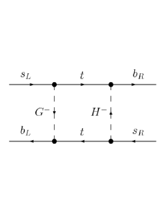
Figure 12: The $\tan^{2}\beta$ enhanced contribution to $C^{LR}_{2}$ arising from charged Higgs and Goldstone boson exchange.

Charged Higgs exchange leads to contributions to all of the operators given in (129)–(131) (with the exception of $\mathcal{O}^{SLL}_{2}$ and its parity flipped counterpart). BLO effects can be easily included by using the matching conditions given in [14] and the corrected vertices given in section 3.2. As an example, the contribution to $C^{LR}_{2}$ arising from the diagram shown in Fig. 12 is given by

$$\delta^{H^{-}}C^{LR}_{2}=\frac{8m_{t}^{4}m_{b}m_{s}\tan^{2}\beta}{m_{H^{+}}^{4}m_{W}^{2}\left(1+\epsilon_{3}\tan\beta\right)^{2}}\left(1+\frac{\Lambda^{R}_{32}}{K_{ts}}\right)H_{3}\left(\frac{m_{W}^{2}}{m_{H^{+}}^{2}},\frac{m_{t}^{2}}{m_{H^{+}}^{2}},\frac{m_{t}^{2}}{m_{H^{+}}^{2}}\right).$$ (135)

(The other contributions undergo similar corrections.) The factor of $\left(1+\epsilon_{3}\tan\beta\right)$ that appears in the denominator acts, once again, to reduce the contributions relative to a LO calculation. The GFM corrections included in the term proportional to $\Lambda^{R}_{32}$, defined in (54), can remove the dependence on the strange quark mass that appears in (135) and lead to potentially large corrections to the MFV result.

The corrected neutral Higgs vertex can give rise to large corrections to $\Delta M_{B_{s}}$ in the large $\tan\beta$ regime via the double Higgs penguin diagrams shown in Fig. 13 [75]. The corresponding matching conditions are

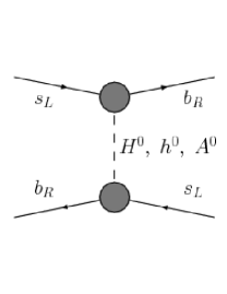
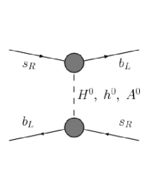
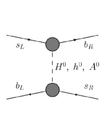
Figure 13: The contributions to $\bar{B}_{s}-B_{s}$ mixing arising from neutral Higgs penguins.

$$C^{SLL}_{1}= -\frac{16\pi^{2}}{2G_{F}^{2}m_{W}^{2}\left(K_{tb}^{\ast}K_{ts}\right)^{2}}\sum_{S^{0}=H^{0},h^{0},A^{0}}\frac{\left(C^{S^{0}}_{L}\right)_{32}\left(C^{S^{0}}_{L}\right)_{32}}{m_{S^{0}}^{2}},$$ (136)

$$C^{LR}_{2}= -\frac{16\pi^{2}}{G_{F}^{2}m_{W}^{2}\left(K_{tb}^{\ast}K_{ts}\right)^{2}}\sum_{S^{0}=H^{0},h^{0},A^{0}}\frac{\left(C^{S^{0}}_{L}\right)_{32}\left(C^{S^{0}}_{R}\right)_{32}}{m_{S^{0}}^{2}}.$$ (137)

The contribution to the parity flipped operator $\mathcal{O}^{SRR}_{1}$ can be obtained via the substitution $L\leftrightarrow R$ in (136). Using the corrected neutral Higgs vertex (66) in the limit of MFV it is easy to obtain the results for $C^{SLL}_{1}$ [14]

$$\left(\delta^{H^{0}}C_{1}^{SLL}\right)^{\rm MFV}=-\frac{G_{F}m_{b}^{2}m_{t}^{4}}{2\sqrt{2}\pi^{2}m_{W}^{2}}\frac{\epsilon_{Y}^{2}\left(16\pi^{2}\right)^{2}\tan^{4}\beta}{\left(1+\epsilon_{s}\tan\beta\right)^{2}\left(1+\epsilon_{3}\tan\beta\right)^{2}}\mathcal{F}^{-}$$ (138)

and $C^{LR}_{2}$

$$\left(\delta^{H^{0}}C_{2}^{LR}\right)^{\rm MFV}=-\frac{G_{F}m_{b}m_{s}m_{t}^{4}}{\sqrt{2}\pi^{2}m_{W}^{2}}\frac{\epsilon_{Y}^{2}\left(16\pi^{2}\right)^{2}\tan^{4}\beta}{\left(1+\epsilon_{s}\tan\beta\right)^{2}\left(1+\epsilon_{3}\tan\beta\right)^{2}}\mathcal{F}^{+}.$$ (139)

Here we decompose the MFV and GFM contributions to the Wilson coefficients in similar manner to (95). We have adopted the notation

$$\mathcal{F}^{\pm}=\frac{\sin^{2}\left(\alpha-\beta\right)}{m_{H^{0}}^{2}}+\frac{\cos^{2}\left(\alpha-\beta\right)}{m_{h^{0}}^{2}}\pm\frac{1}{m_{A^{0}}^{2}}$$ (140)

to represent the interference between the scalar and pseudoscalar contributions. At large $\tan\beta$, (140) becomes (for $m_{A}^{2}>m_{Z}^{2}$)

$$\mathcal{F}^{\pm}=\frac{1}{m_{H^{0}}^{2}}\pm\frac{1}{m_{A^{0}}^{2}},$$ (141)

and the scalar and pseudoscalar contributions to $C^{SLL}_{1}$ approximately cancel, whilst the contributions to $C^{LR}_{2}$ interfere constructively. As has been pointed out in [76, 14], the double penguin contribution to $C^{LR}_{2}$ acts to reduce the value of $\Delta M_{B_{s}}$, bringing it closer to the current experimental limit (126). The factor of $m_{s}$ that appears (139) suppresses the contribution somewhat, however it can still be of the order of 50% of the Standard Model contribution in certain regions of parameter space even once the current limits on $\bar{B}_{s}\to\mu^{+}\mu^{-}$ are taken into account [14].

Including the effects of GFM when evaluating the contributions to the Wilson coefficients $C^{SLL}_{1}$ and $C^{LR}_{2}$ can lead to far more varied effects. The full expressions for $C^{LR}_{2}$ and $C^{SLL}_{1}$ can be obtained by using (65)–(67), however, as they are rather complicated, let us highlight the phenomenologically most interesting terms that appear. If the insertion $\delta_{LL}^{d}$ is non–zero the contribution to $C^{LR}_{2}$ becomes

$$\left(\delta^{H^{0}}C^{LR}_{2}\right)^{\rm LL}=-\frac{m_{b}m_{s}}{2\pi^{2}g_{2}^{2}\left(K_{tb}^{\ast}K_{ts}\right)^{2}}\frac{\epsilon_{LL}^{2}x_{\widetilde{d}_{L}}^{2}\left(16\pi^{2}\right)^{2}\tan^{4}\beta}{\left(1+\epsilon_{s}\tan\beta\right)^{2}\left(1+\epsilon_{3}\tan\beta\right)^{2}}\mathcal{F}^{+}\left(\delta_{LL}^{d}\right)^{2}.$$ (142)

In a similar manner to the MFV correction (139), the contribution acts to reduce the value of $\Delta M_{B_{s}}$. Once again, however, $C_{2}^{LR}$ is suppressed by a factor of the strange quark mass that tends to limit the size of the correction to $\Delta M_{B_{s}}$. The insertion $\delta_{LR}^{d}$ also contributes to $C_{2}^{LR}$ via the diagram where one penguin is mediated by gluino exchange and the other is mediated by chargino exchange

$$\left(\delta^{H^{0}}C^{LR}_{2}\right)^{\rm LR}=-\frac{m_{s}m_{\widetilde{g}}m_{t}^{2}}{4\pi^{2}m_{W}^{2}K_{tb}^{\ast}K_{ts}}\frac{\epsilon_{RL}\epsilon_{s}\epsilon_{Y}x_{\widetilde{d}_{RL}}\left(16\pi^{2}\right)^{2}\tan^{4}\beta}{\left(1+\epsilon_{s}\tan\beta\right)^{2}\left(1+\epsilon_{3}\tan\beta\right)}\mathcal{F}^{+}\delta_{LR}^{d}.$$ (143)

In this case the contribution can increase or decrease the value of $\Delta M_{B_{s}}$ depending on the sign of $\delta_{LR}^{d}$. However the factor of $m_{s}$ that appears in (143) means that these effects are, once again, rather small.

It is possible to avoid factors of the strange quark mass that appear in the above expressions for $C_{2}^{LR}$ by considering scenarios where the right handed Higgs coupling that appears in (137) does not feature such a suppression. This occurs if either $\delta_{RL}^{d}$ or $\delta_{RR}^{d}$ are non–zero. If we consider the diagram where one Higgs penguin is mediated by chargino exchange and the other by gluino exchange we have, for non–zero $\delta_{RR}^{d}$ [17]

$$\left(\delta^{H^{0}}C^{LR}_{2}\right)^{\rm RR}=-\frac{m_{b}^{2}m_{t}^{2}}{4\pi^{2}m_{W}^{2}K_{tb}^{\ast}K_{ts}}\frac{\epsilon_{RR}\epsilon_{Y}x_{\widetilde{d}_{R}}\left(16\pi^{2}\right)^{2}\tan^{4}\beta}{\left(1+\epsilon_{s}\tan\beta\right)\left(1+\epsilon_{3}\tan\beta\right)^{3}}\mathcal{F}^{+}\delta_{RR}^{d}.$$ (144)

A similar contribution is possible for the insertion $\delta_{RL}^{d}$

$$\left(\delta^{H^{0}}C^{LR}_{2}\right)^{\rm RL}=-\frac{m_{b}m_{\widetilde{g}}m_{t}^{2}}{4\pi^{2}m_{W}^{2}K_{tb}^{\ast}K_{ts}}\frac{\epsilon_{RL}\epsilon_{3}\epsilon_{Y}x_{\widetilde{d}_{RL}}\left(16\pi^{2}\right)^{2}\tan^{4}\beta}{\left(1+\epsilon_{s}\tan\beta\right)\left(1+\epsilon_{3}\tan\beta\right)^{2}}\mathcal{F}^{+}\delta_{RL}^{d}.$$ (145)

As one penguin is mediated by chargino exchange, (144)–(145) feature only a linear dependence on $\delta_{RR}^{d}$ and $\delta_{RL}^{d}$. Large positive or negative contributions to $\Delta M_{B_{s}}$ are therefore possible, depending on the sign of the insertions.

If $\delta_{LL}^{d}$ or $\delta_{LR}^{d}$ are non–zero, in addition to either $\delta_{RL}^{d}$ or $\delta_{RR}^{d}$ the diagram involving two gluino mediated penguins becomes viable. For example, if $\delta_{LL}^{d}$ and $\delta_{RR}^{d}$ are non–zero we have the contribution

$$\left(\delta^{H^{0}}C^{LR}_{2}\right)^{\rm LL+RR}=-\frac{m_{b}^{2}}{2\pi^{2}g_{2}^{2}\left(K_{tb}^{\ast}K_{ts}\right)^{2}}\frac{\epsilon_{RR}\epsilon_{LL}x_{\widetilde{d}_{L}}x_{\widetilde{d}_{R}}\left(16\pi^{2}\right)^{2}\tan^{4}\beta}{\left(1+\epsilon_{s}\tan\beta\right)\left(1+\epsilon_{3}\tan\beta\right)^{3}}\mathcal{F}^{+}\delta_{LL}^{d}\delta_{RR}^{d}.$$ (146)

Similar contributions arise for the remaining combinations LL+RL, LR+RR and LR+RL. The $\tan^{4}\beta$ dependence of (146), coupled with its dependence on the strong coupling constant present in the factors of $\epsilon_{LL}$ and $\epsilon_{RR}$, can lead to large corrections to $\Delta M_{B_{s}}$ in the large $\tan\beta$ regime. We should briefly mention here how this result compares to that presented in [62]. As discussed in [17] the authors of [62] omit the effects that arise when considering the GFM contributions to the bare CKM matrix (79). Once one takes into account such contributions, one of the factors of $\left(1+\epsilon_{3}\tan\beta\right)$ that appears in Eq. (5.8) of [62] is replaced by a factor of $\left(1+\epsilon_{s}\tan\beta\right)$. Taking this correction into account, our results agree.

A common feature of all of these corrections lie in the factors of $\left(1+\epsilon_{3}\tan\beta\right)$ and $\left(1+\epsilon_{s}\tan\beta\right)$ that appear in the denominators of all double Higgs penguin contributions. These factors represent the resummation of $\tan\beta$ enhanced effects and act to reduce the contributions for $\mu>0,~{}A_{t}<0$ compared to calculations where resummation is not taken into account.

6.2 BLO Corrections to SUSY Contributions in the MIA

The supersymmetric contributions to $\bar{B}_{s}-B_{s}$ mixing proceed via box diagrams mediated by gluino, chargino and neutralino exchange. Unlike the decay $\bar{B}\to X_{s}\gamma$ however, sizeable effects due to these contributions are often limited to regions where the squarks and gluinos are relatively light $\mathcal{O}\left(500\,\mbox{GeV}\right)$.

As $\bar{B}_{s}-B_{s}$ mixing is a $\Delta F=2$ process, the gluino and neutralino contributions, at LO, feature combinations of two insertions. The LO gluino matching conditions have been discussed, in the context of the MIA, in [73]. It is relatively easy to modify them to take into account the BLO effects discussed in section 2 by using the recipe discussed at the end of subsection 4.2. The gluino contribution to the operator $C_{2}^{LR}$ is given by (to second order in the MIA)

$$\left(\delta^{\widetilde{g}}C_{2}^{LR}\right)^{\rm GFM}=\frac{16\alpha_{s}^{2}\sin^{4}\theta_{W}}{9\alpha^{2}\left(K_{tb}^{\ast}K_{ts}\right)^{2}}\frac{m_{W}^{2}}{m_{\widetilde{g}}^{2}}\Bigg{\{}\frac{11\left(1+\epsilon_{Y}Y_{t}^{2}\tan\beta\right)f_{\widetilde{g}}^{[2]}\left(x_{\widetilde{d}}\right)}{\left(1+\epsilon_{s}\tan\beta\right)\left(1+\epsilon_{3}\tan\beta\right)}\delta_{LR}^{d}\delta_{RL}^{d}$$

$$+\left[-42f_{\widetilde{g}}^{[1]}\left(x_{\widetilde{d}}\right)+\left(6+11\frac{\mu^{2}m_{b}^{2}}{m_{\widetilde{g}}^{2}}\frac{\epsilon_{LL}\epsilon_{RR}\tan^{4}\beta}{\left(1+\epsilon_{s}\tan\beta\right)\left(1+\epsilon_{3}\tan\beta\right)^{3}}\right)f_{\widetilde{g}}^{[2]}\left(x_{\widetilde{d}}\right)\right]\delta_{LL}^{d}\delta_{RR}^{d}\Bigg{\}}.$$ (147)

The functions $f_{\widetilde{g}}^{[1,2]}\left(x_{\widetilde{d}}\right)$ are given in appendix A.4 and $x_{\widetilde{d}}$ is defined in (97). Once again, we see that the contributions arising from the insertions $\delta_{LR}^{d}$ and $\delta_{RL}^{d}$ are modified in the same manner as the supersymmetric contributions to $\bar{B}\to X_{s}\gamma$ (namely (99) and (100)) that appear in section 4.2. The inclusion of BLO effects therefore tends to reduce the overall contribution to $C_{2}^{LR}$ arising from these insertions. The BLO term proportional to $\delta_{LL}^{d}\delta_{RR}^{d}$, on the other hand, tends to interfere with terms that arise at fourth order in the MIA and on the whole tends to be rather small. In addition, the combinations $\delta_{LL}^{d}\delta_{RL}^{d}$ and $\delta_{LR}^{d}\delta_{RR}^{d}$ also appear once BLO effects are taken into account. Due to their $\tan^{2}\beta$ dependence, they can viably compete with the corresponding terms that arise at higher orders in the MIA. Contributions arising from MFV corrections to the bare mass matrix can also appear and play the rôle of $\delta_{LL}^{d}$ and $\delta_{LR}^{d}$ insertions. (Contributions where the MFV corrections play the rôle of $\delta_{RL}^{d}$ and $\delta_{RR}^{d}$ insertions are suppressed by factors of $m_{s}$.)

Turning to the contributions arising from chargino box diagrams, in MFV the dominant behaviour at LO arises from contributions to the Wilson coefficient $C^{VLL}$. At large values of $\tan\beta$, however, large corrections to $C_{1,2}^{SLL}$ are possible that interfere destructively with $C^{VLL}$ and can reduce the contribution that arises from chargino box diagrams to $\Delta M_{B_{s}}$ [14]. The inclusion of BLO effects in MFV, however, tends to reduce this cancellation somewhat; whilst the Wilson coefficient $C^{VLL}$ remains virtually unaffected by BLO corrections, the BLO corrections to $C_{1,2}^{SLL}$ introduce factors of $\left(1+\epsilon_{3}\tan\beta\right)$ that, in the phenomenologically favoured region $\mu>0$ and $A_{t}<0$, act to reduce the contribution to the Wilson coefficient. These effects therefore reduce the cancellations that occur between the two Wilson coefficients, and can lead to an enhancement of the contributions that arise from chargino box diagrams [14].

In the GFM scenario, the occurrence of the bare mass matrix in the chargino vertex 35 can play the rôle of one (or both) of the factors of $K_{ts}$ that mediate the flavour change in the leading order matching conditions. A dependence on the flavour violating parameters $\delta^{d}_{XY}$ can therefore appear once one proceeds beyond the LO. In particular, the factor of $m_{s}$, that features in the matching condition for $C_{2}^{LR}$ in MFV, can be bypassed in the GFM scenario if either $\delta_{RL}^{d}$ or $\delta_{RR}^{d}$ are non–zero. A similar effect occurs for the Wilson coefficients $C_{1,2}^{SLL}$, where non–zero $\delta_{LL}^{d}$ or $\delta_{LR}^{d}$ can lead to additional contributions to the coefficient. It is therefore possible to enhance, or decrease, the cancellations that occur between $C^{VLL}$ and the remaining Wilson coefficients depending on the sign of the insertions $\delta^{d}_{XY}$.

The appearance of the bare mass matrix in the neutralino vertex also introduces additional BLO corrections that can modify the LO contributions. In a similar manner to the contributions to the decay $\bar{B}\to X_{s}\gamma$, these corrections typically manifest themselves as factors of $(1+\epsilon_{3}\tan\beta)$ or $(1+\epsilon_{s}\tan\beta)$ and tend to reduce the contributions compared to a LO analysis.

Let us finally comment on the RG running of the SUSY corrections. The six flavour anomalous dimension matrix required to evolve the Wilson coefficients from the SUSY matching scale to the electroweak scale was given in [68]. If we consider the running of the coefficient $C_{2}^{LR}$ we have

$$\delta C_{2}^{LR}\left(\mu_{W}\right)=\delta C_{2}^{LR}\left(\mu_{SUSY}\right)+\frac{\alpha_{s}\left(\mu_{W}\right)}{\pi}\left[2\delta C_{2}^{LR}\left(\mu_{SUSY}\right)-\frac{3}{2}\delta C_{1}^{LR}\left(\mu_{SUSY}\right)\right]\log\frac{\mu_{SUSY}^{2}}{\mu_{W}^{2}}.$$ (148)

In contrast to the decay $\bar{B}\to X_{s}\gamma$, the RG evolution of the Wilson coefficients, from $\mu_{SUSY}$ to $\mu_{W}$, acts to increase the coefficients with respect to an analysis where RG running is ignored. A similar effect exists in the SLL sector. In the VLL sector, however, RG running acts to decrease the Wilson coefficients in a similar manner to $\bar{B}\to X_{s}\gamma$. These effects can therefore act to enhance the cancellations between contributions to the VLL sector and the remaining operators.

6.3 Full Calculation

Let us now discuss the calculation we perform in our numerical analysis. Following the method discussed at the end of section 4, we evaluate the SM matching conditions to NLO using the matching conditions originally given in [65]. For the charged Higgs contribution, we use the corrected vertices given in appendix D when evaluating the LO matching conditions given in [14]. When evaluating the SUSY contributions we use the LO matching conditions collected in [9] (transformed into our operator basis). They are then subsequently evolved from the SUSY matching scale to the EW scale using the NLO anomalous dimension matrix given in [68].

In summary, in this section we have discussed the effects of all the dominant BLO corrections to $\bar{B}_{s}-B_{s}$ mixing. In particular, we have considered all the contributions that arise once one takes into account the double Higgs penguin contribution. In the region where $\tan\beta$ and the sparticle masses are large, for example, these contributions can dominate the corrections to $\Delta M_{B_{s}}$ that arise from new physics, due to the non–decoupling property of the corrections to the neutral Higgs vertex. Turning to the supersymmetric contributions to the process, we see that, although they play a more minor rôle compared to the neutral Higgs contributions in the large $\tan\beta$ regime, the overall effect of BLO corrections is to reduce the contributions arising from gluino exchange. We have also seen that, in contrast to the decay $\bar{B}\to X_{s}\gamma$, RG evolution between $\mu_{SUSY}$ and $\mu_{W}$ can act to enhance the contributions of the coefficient $C_{2}^{LR}$ in particular.

7 Numerical Results

Before proceeding with our numerical results let us first define our parameterisation for the soft sector. We treat the soft terms (12), defined in the physical SCKM basis, as input. For the diagonal elements we set

$$\left(m_{d,LL}^{2}\right)_{ii} =m_{\widetilde{q}}^{2}\;\delta_{ii}, \left(m_{d,RR}^{2}\right)_{ii} =m_{\widetilde{q}}^{2}\;\delta_{ii}, \left(m_{d,LR}^{2}\right)_{ii} =A_{d}\left(m_{d}\right)_{ii},$$ (149)

The off–diagonal elements are related to the parameters $\delta_{XY}^{d}$ via the relations defined in (20)–(21). The soft terms in the up–sector are defined analogously. As inputs for the Higgs sector we take $m_{A}$, $\mu$ and $\tan\beta$ and use FeynHiggs 2.2.8 [77] to determine the remaining parameters. For the majority of this section we will only vary one $\delta_{XY}^{d}$ at a time unless stated otherwise. Finally the gaugino soft terms $M_{1}$ and $M_{2}$ are related to the gluino mass $m_{\widetilde{g}}$ via the usual unification relation.

Let us briefly specify the abbreviations used to denote the various approximations used in this section:

• LO: a calculation that does not feature the resummation procedure described in section 2. We do, however, include the LO effects that arise from RG evolution from $\mu_{SUSY}$ to $\mu_{W}$ (in contrast with [16]);

• $\widetilde{g}$–BLO: the approximation used in [16] where only gluino contributions were taken into account in the resummation procedure;

• BLO: the results obtained using the full expressions included in appendix D.

7.1 $\bar{B}\to X_{s}\gamma$

A detailed analysis of the BLO effects relevant to $\bar{B}\to X_{s}\gamma$ was presented in [16] and we shall therefore tend to focus on the additional effects induced by the inclusion of electroweak contributions. We shall also compare the approximate expressions, gathered in section 4, with our complete calculation.

Before focusing on the GFM scenario,

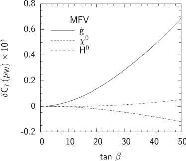
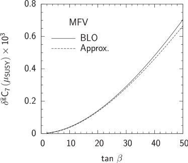
Figure 14: The panel on the left depicts corrections to the Wilson coefficient $C_{7}$ induced by gluino, neutralino and neutral Higgs exchange for MFV. The panel on the right illustrates the behaviour of the approximate result (96) compared with the full numerical calculation. The soft sector is parameterised as follows: $m_{\widetilde{q}}=1\,\mbox{TeV}$, $m_{\widetilde{g}}=\sqrt{2}\,m_{\widetilde{q}}$, $A_{t}=-500\,\mbox{GeV}$, $m_{A}=500\,\mbox{GeV}$, $\mu=500\,\mbox{GeV}$.

let us briefly consider the effects induced by the bare mass matrix and corrected Higgs vertices in the case of MFV. The panel on the left of Fig. 14 illustrates the contributions mediated by gluinos, neutralinos and neutral Higgs. As is evident from the graph, all three contributions are rather small and, compared with the corrections to $C_{7}$ induced by charged Higgs or chargino exchange, are of the order of a few percent. However, it should be noted that the gluino and neutralino contributions are both larger than the neutral Higgs contribution in this particular region of parameter space. The panel on the right of Fig. 14 depicts the approximate expression (96) alongside the result taken from our numerical analysis. As is evident, (96) describes the behaviour of the full numerical result rather well for this choice of parameters and only differs by about 5% from the result of a full numerical calculation at large $\tan\beta$.

Now let us turn to the GFM scenario.

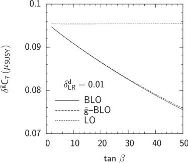
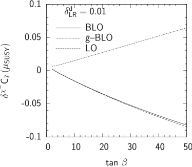
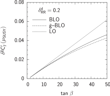
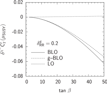
Figure 15: The corrections to the Wilson coefficient $C_{7}$ (evaluated at the scale $\mu_{SUSY}$) induced by gluino exchange (on the left) and chargino exchange (on the right). $\delta_{LR}^{d}=0.01$ and $\delta_{RR}^{d}=0.2$ in the top and bottom panels, respectively. The soft sector is described by the same parameters as Fig. 14. As stated at the beginning of section 7, LO is used to denote a calculation that does not take into account the BLO effects discussed in section 2. $\widetilde{g}$–BLO denotes the approximation used in [15] where only gluino contributions are taken into account in the resummation procedure. BLO is used to denote the results obtained using the expressions collected in appendix D.

As stated in sections 4.1 and 4.2, it is possible, once BLO effects are taken into account, that large cancellations can occur between the various supersymmetric contributions. The top two plots in Fig. 15, for example, illustrate the cancellations that occur between the chargino and gluino contributions for non–zero $\delta_{LR}^{d}$. The dominant BLO chargino contributions to $C_{7}$ stem from the appearance of the bare mass matrix in the modified chargino vertex (36)–(37). The inclusion of electroweak effects, as indicated by the absence of a term dependent on $\epsilon_{Y}$ in the terms proportional to $\delta_{LR}^{d}$ in (99) and (104), is rather small. The lower two plots in Fig. 15 show the contributions in the primed sector for non–zero $\delta_{RR}^{d}$. Here we see a similar cancellation between the BLO effects arising from the chargino contribution and gluino contribution to $C_{7}^{\prime}$. The effect of including electroweak effects is, however, larger than the case of the LR insertion due to the appearance of $\left(1+\epsilon_{3}\tan\beta\right)$ (rather than $\left(1+\epsilon_{s}\tan\beta\right)$) in the denominators of (101) and (106). However, one can see from the two graphs that the increase in the gluino contribution tends to be compensated by a similar correction to the chargino contribution. As such the overall effect on the branching ratio is rather small.

Let us briefly discuss how well the MIA expressions presented in section 4 describe the results of our numerical analysis. The two panels in Fig. 16

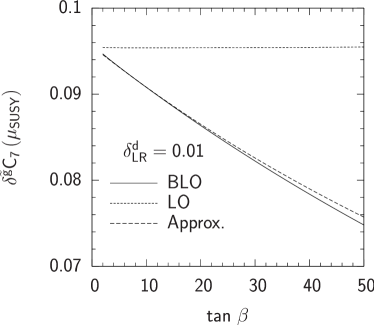
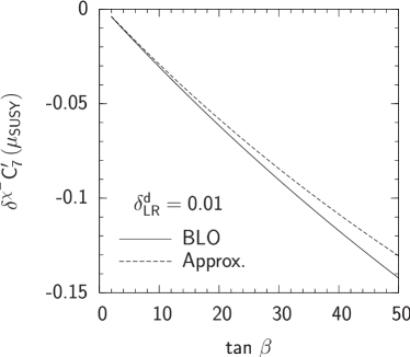
Figure 16: Plots comparing of the results of our full numerical calculation with the analytic results, derived in the MIA, given in section 4. The gluino contribution is shown in the panel on the left, whilst the chargino contribution is shown in the panel on the right. $\delta_{LR}^{d}=0.01$ in both figures whilst the remaining parameters are described in the caption of Fig. 14. The MFV contribution to the Wilson coefficient in question has been removed in both panels.

show the approximate expressions for the gluino (99) and chargino (104) contributions, alongside the results of our full numerical analysis, performed in the mass eigenstate formalism where flavour violation is communicated via the unitary matrices (19). As is evident from the graph, in this region of parameter space at least, the agreement between the approximate expression and that of the full calculation is rather good (within 10%). We have checked that expressions for the chargino and gluino contributions that arise from the remaining insertions also tend to agree within a similar accuracy.

Now let us consider the effect of including electroweak corrections when computing the corrected charged Higgs vertex (51)–(52).

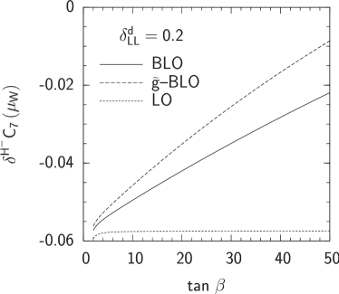
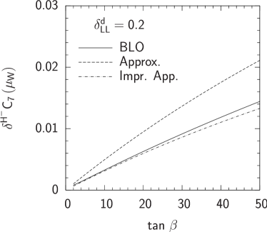
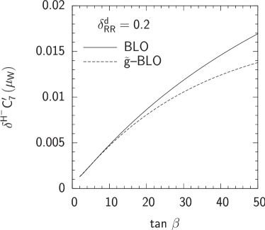
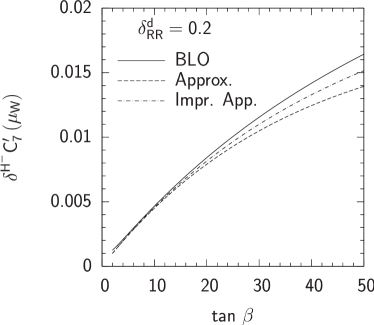
Figure 17: The corrections to the Wilson coefficient $C_{7}$ arising from charged Higgs exchange. In the top two panels $\delta_{LL}^{d}=0.2$ whilst in bottom panels $\delta_{RR}^{d}=0.2$. LO, BLO and $\widetilde{g}$ are defined in the caption of Fig. 15. In the panels to the right our analytic results are compared with those of our complete numerical analysis. The MFV contributions to $C_{7}$ and $C_{7}^{\prime}$ arising from charged Higgs exchange have been removed in the panels to the right. The abbreviation “Approx.” denotes the results gathered in section 4.1, whilst “Impr. App.” is used to denote the same results supplemented by the substitutions gathered in subsection 3.3. The soft sector is described by the same parameters as Fig. 14.

The panel on the top–left of Fig. 17, illustrates the effect of including BLO corrections when calculating the charged Higgs mediated contribution to $C_{7}$, for non–zero $\delta_{LL}^{d}$. If $\delta_{LL}^{d}$ is positive, the GFM corrections to the charged Higgs vertex tend to interfere constructively with the MFV contribution, reducing the charged Higgs contribution to $C_{7}$ compared to a LO analysis. On the other hand, if $\delta_{LL}^{d}$ is negative, the MFV and GFM corrections to the LO contribution interfere destructively and can therefore lead to an enhancement of the charged Higgs contribution to the decay. As $A_{b}$ is set equal to zero, the bulk of the difference induced by the inclusion of EW contributions in the figure results from the correction to the right handed coupling (52) and the corrections that arise from the additional gaugino mediated electroweak effects discussed in subsection 3.3. This is confirmed in the top–right panel that illustrates the behaviour of the approximate expression (90) compared with the results of our full numerical calculation. As is evident from the figure, the agreement between the curves is rather poor and the approximate result where the electroweak couplings $g_{1}$ and $g_{2}$ are ignored provides a 30% overestimate of the beyond leading order effects. The origin of this discrepancy stems from graphs featuring gaugino exchange. This result is not specific to the GFM scenario and such effects have been discussed before, in the context of MFV in [14]. Once one takes into account these effects, by applying the substitutions found in subsection 3.3, the agreement between the numerical and approximate results improves dramatically. As is evident from the line depicting the improved approximation in the top–right panel of Fig. 17.

The lower two panels in Fig. 17 depict the contributions to the primed coefficients arising from BLO corrections to charged Higgs exchange for $\delta_{RR}^{d}=0.2$. In a similar manner to the insertion $\delta_{LL}^{d}$, the majority of the difference between the effects considered in [16] (the line labeled $\widetilde{g}$–BLO) and the complete calculation presented in this analysis, stems from the destructive interference between the $\epsilon_{s}$ and $\epsilon_{Y}$ terms that appear in the denominator of (52) and the additional electroweak corrections to the $(3,3)$ element of the left–handed charged Higgs vertex. Both of these effects act to increase the charged Higgs contribution attributable to RR insertions. This situation is also evident in the lower right panel, where the inclusion of the additional electroweak corrections described in subsection 3.3 roughly doubles the accuracy of the approximate expression.

The contributions due to new physics for each insertion are shown in Fig. 18.

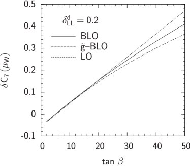
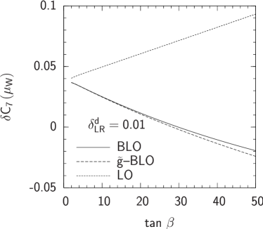
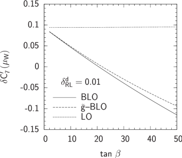
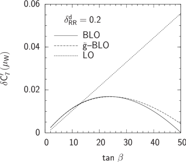
Figure 18: The corrections to the Wilson coefficients $C_{7}$ (the top two panels) and $C_{7}^{\prime}$ (the lower two panels) due to contributions beyond the SM. The soft sector is described by the same parameters as Fig. 14.

As is evident from the plots for the LR, RL and RR insertions, the effect of BLO corrections tends to be rather large. For example, in the case of the LR insertion (the top–right panel in Fig. 18), the reduction of the gluino contribution with increasing $\tan\beta$, coupled with its destructive interference with the chargino contribution, can dramatically alter the behaviour of the Wilson coefficient for even moderate $\tan\beta$. Similar effects occur for the RL and RR insertions. For the LL insertion the difference between the LO and BLO calculations shown in the top–left panel of Fig. 18 is rather slight. This is because a $\tan\beta$ enhanced correction, proportional to $\delta_{LL}^{d}$, appears at LO in the chargino Wilson coefficients. It is therefore rather difficult for the BLO corrections to the chargino contribution to play as large a rôle as they do for the other three insertions.

Finally, let us consider the combined effect these contributions have on the branching ratio. Fig. 19

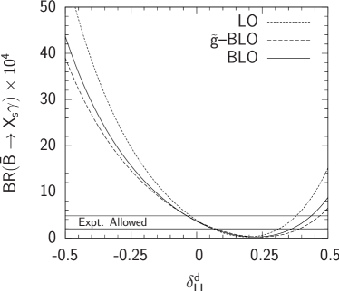
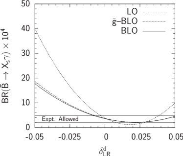
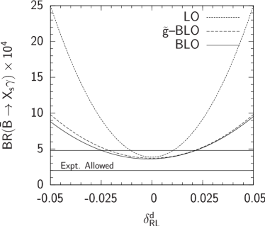
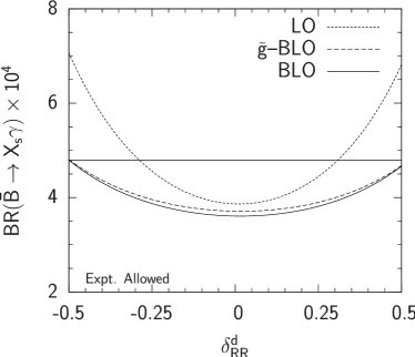
Figure 19: The variation of BR$(\bar{B}\to X_{s}\gamma)$ with the flavour violating parameters $\delta_{XY}^{d}$. The soft sector is parameterised as follows $m_{\widetilde{q}}=1\,\mbox{TeV}$, $m_{\widetilde{g}}=m_{\widetilde{q}}\,/\sqrt{2}$, $A_{u}=-500\,\mbox{GeV}$, $m_{A}=500\,\mbox{GeV}$, $\mu=500\,\mbox{GeV}$ and $\tan\beta=50$. A broad region in agreement with the current experimental limit is shown in all four panels.

illustrates the variation of the branching ratio with the flavour violating parameters $\delta_{XY}^{d}$. As is evident from the figure, BLO effects can be significant for all four insertions. Contributions due to flavour violation in the LR and RL sectors, in particular, can undergo reductions by up to a factor of two compared to a LO analysis. Turning to the inclusion of electroweak effects, we see that although such corrections can effect the Wilson coefficients by up to 30%, the overall difference between the approximation used in [16] and the full calculation used in this analysis is rather small. This is primarily because the origin of the large discrepancy, between the LO and BLO calculations, is mainly due to the cancellation between the gluino and chargino contributions, that arise for each insertion. As both the chargino and gluino contributions undergo similar corrections, once electroweak effects are taken into account, the overall effect on the branching ratio tends to be rather minor.

Fig. 20 depicts the variation of the branching ratio with $\tan\beta$.

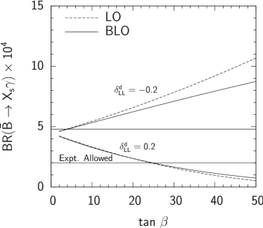
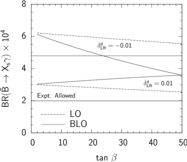
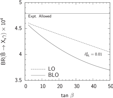
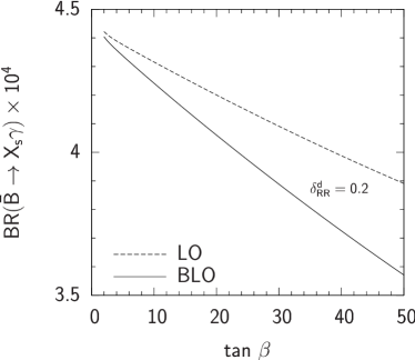
Figure 20: The variation of BR$(\bar{B}\to X_{s}\gamma)$ with the $\tan\beta$. The soft sector is parameterised as follows $m_{\widetilde{q}}=1\,\mbox{TeV}$, $m_{\widetilde{g}}=\sqrt{2}m_{\widetilde{q}}$, $A_{u}=-500\,\mbox{GeV}$, $m_{A}=500\,\mbox{GeV}$ and $\mu=500\,\mbox{GeV}$. A broad region in agreement with the current experimental limit is also shown when applicable.

All four panels exhibit the focusing effect first described in [15, 16] where BLO corrections act to reduce the LO result such that the SM result (86) is preferred. Once again we see that for the insertion $\delta_{LL}^{d}$ BLO corrections are rather small due to the presence of the LO correction to the chargino contribution in (102). For the remaining insertions we see that the BLO effects described in this paper can significantly alter LO corrections for $\tan\beta$ as low as 20.

In summary, we have seen that whilst electroweak corrections can effect individual Wilson coefficients by up to 20%, the overall effect of such contributions is rather small. In particular, the focusing effect described in [15, 16] remains even once one includes all the electroweak corrections described in this paper. This is unsurprising as the focusing effect mainly arises from the combined effect of two contributions. The first arises from renormalization group evolution of the Wilson coefficients evaluated at the SUSY scale to the electroweak scale, which is naturally independent of electroweak corrections. The second is due to cancellations between the gluino and chargino contributions to the decay. We have seen however that electroweak corrections typically alter each contribution in a similar manner, and an increase in the gluino contribution, attributable to the destructive interference of the gluino and chargino contributions to the bare mass matrix, is often accompanied by a similar increase in the chargino contribution. Finally, we have seen that the approximate expressions gathered in section 4 tend to describe the overall behaviour of the supersymmetric contributions rather well. The contributions arising from the charged Higgs exchange however, often have to be modified according to the improved approximation described in subsection 3.3 to obtain a sufficient level of accuracy.

7.2 $\bar{B}_{s}\to\mu^{+}\mu^{-}$

As discussed in section 5, large corrections to the decay $\bar{B}_{s}\to\mu^{+}\mu^{-}$ are possible in the large $\tan\beta$ regime due to the contributions of scalar and pseudoscalar operators that are proportional to $\tan^{3}\beta$. Fig. 21

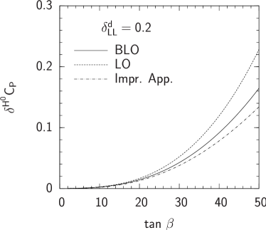
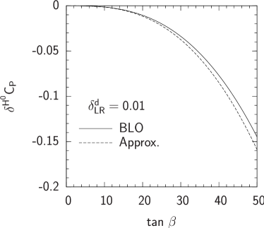
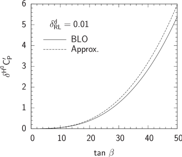
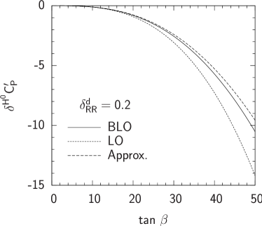
Figure 21: The $\tan\beta$ dependence of the Wilson coefficients $C_{P}$ and $C_{P}^{\prime}$. In the top two panels $\delta_{LL}^{d}=0.2$ and $\delta_{LR}^{d}=0.01$, respectively, whilst in the lower two $\delta_{RL}^{d}=0.01$ and $\delta_{RR}^{d}=0.2$. In all four panels the MFV contributions to $C_{P}^{(\prime)}$ have been removed. The soft sector is parameterised as follows $m_{\widetilde{q}}=1\,\mbox{TeV}$, $m_{\widetilde{g}}=\sqrt{2}m_{\widetilde{q}}$, $A_{u}=-500\,\mbox{GeV}$, $m_{A}=500\,\mbox{GeV}$, $\mu=500\,\mbox{GeV}$. The abbreviation “Approx.” is used to denote the contributions arising from formulae (123)–(124) whilst “Imp. Appr.” is used to denote the calculation that includes the additional electroweak contribution (125).

depicts the dependence of our analytic and numerical results for the Wilson coefficients $C_{P}$ and $C_{P}^{\prime}$ on $\tan\beta$ for various choices of flavour violating parameters. The top–left panel in the figure shows the contribution due to the insertion $\delta_{LL}^{d}$. Let us point out that when one only uses expression (123) to calculate the contribution to $C_{P}$, one obtains a value roughly 20% larger than the result obtained from a full numerical analysis. Once one takes into account the additional LO correction induced by gaugino–higgsino mixing (125) (denoted by Impr. App. in Fig. 21) the agreement improves to roughly 10%. The remaining sources of discrepancy are mainly due to wavefunction corrections to the bare mass matrix, which can be as large as 10%, and the inevitable limitations associated with the MIA. The contributions due to the insertions $\delta_{LR}^{d}$ and $\delta_{RL}^{d}$ shown in the top–right and bottom–left figures respectively are absent at LO as the effects of the insertions cancel [17]. However, once BLO effects are taken into account, a dependence on the insertions is reintroduced due to their appearance in the bare mass matrix (45). (The $\delta_{LR}^{d}$ dependence of (45) becomes apparent once one recalls that $\left(\delta_{LR}^{d}\right)_{23}=\left(\delta_{RL}^{d}\right)_{32}$.) Comparing the approximate and numerical results for the BLO corrections we see that they typically agree with one another very well. (Unlike the $\delta_{LL}^{d}$ insertion, contributions due to wavefunction corrections are typically rather small as they appear at second order in the MIA and tend to be suppressed by factors of $m_{b}^{2}$.) Finally, the bottom–right panel shows the contributions that arise for non–zero $\delta_{RR}^{d}$ where, once again, the analytic and numerical results agree with one another rather well.

With these results in mind let us now consider the overall effect of such corrections on the branching ratio of the decay. Fig. 22 depicts the dependence the branching ratio on the various sources of flavour violation in the squark sector. The two graphs depicting the variation with $\delta_{LL}^{d}$ and $\delta_{RR}^{d}$ show the characteristic suppression associated with the BLO factors of $\left(1+\epsilon_{3}\tan\beta\right)$ and $\left(1+\epsilon_{s}\tan\beta\right)$ that appear in the denominators of the Wilson coefficients (122)–(124). This suppression can loosen the bounds placed on these insertions by the $\bar{B}_{s}\to\mu^{+}\mu^{-}$ constraint. The panel depicting the variation with $\delta_{LL}^{d}$ displays a larger dependence on the the gluino mass than the panel featuring the insertion $\delta_{RR}^{d}$ as the gluino mass not only features in the gluino contribution, but also in the corrections that arise once one includes gaugino–higgsino mixing. (We remind the reader that we assume that the mass of the wino and the gluino are related.) Let us briefly comment however, that in contrast to $\bar{B}\to X_{s}\gamma$, the differences between the BLO and LO results for MFV and GFM calculations tend to be rather similar. This is because, now, the only dominant contribution to the decay is via the neutral Higgs penguin and BLO effects tend to be limited to the factors of $(1+\epsilon_{s}\tan\beta)$ and $(1+\epsilon_{3}\tan\beta)$ that accompany the LO matching conditions. Turning to the $\delta_{LR}^{d}$ and $\delta_{RL}^{d}$ insertions, large deviations from a purely leading order calculation are possible due to the reappearance of the insertion in the Wilson coefficients (123)–(124) once one proceeds beyond the LO [17].

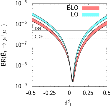
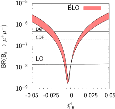
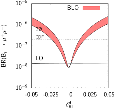
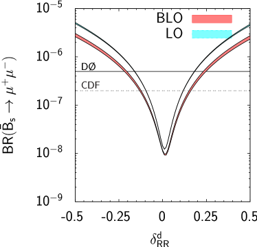
Figure 22: The dependence of BR($\bar{B}_{s}\to\mu^{+}\mu^{-}$) on $\delta_{XY}^{d}$ for $m_{\widetilde{q}}=1\,\mbox{TeV}$, $A_{u}=-500\,\mbox{GeV}$, $m_{A}=500\,\mbox{GeV}$, $\mu=500\,\mbox{GeV}$ and $\tan\beta=50$. The light blue (light grey) and red (dark grey) bands depict the effect of varying $m_{\widetilde{g}}$ between $m_{\widetilde{q}}/\sqrt{2}$ and $\sqrt{2}m_{\widetilde{q}}$. The published DØ and preliminary CDF limits for the decay are shown.

Finally, the asymmetric nature of the $\delta_{LL}^{d}$ and $\delta_{LR}^{d}$ curves arises as these contributions interfere directly with the MFV contribution and it is therefore possible to induce quite large cancellations. For $\delta_{RR}^{d}$ and $\delta_{RL}^{d}$ on the other hand, direct interference with the MFV contributions is generally not possible. Cancellations with the Wilson coefficient $C_{A}$ when calculating the branching ratio (117) can occur, however, and lead the minima of the curves to deviate slightly from MFV. In general however, in a similar manner to $\bar{B}\to X_{s}\gamma$, the overall effect of these insertions is to increase the branching ratio with respect to the MFV result, independent of the sign of the insertion.

The dependence of the branching ratio on $\tan\beta$ and the pseudoscalar mass $m_{A}$ is shown in Fig. 23.

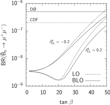
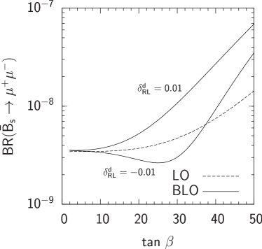
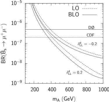
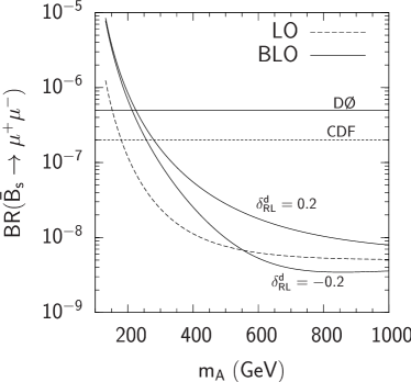
Figure 23: The dependence of BR($\bar{B}_{s}\to\mu^{+}\mu^{-}$) on $\tan\beta$ (the top two panels) and $m_{A}$ (the bottom two panels). The soft sector is parameterised as follows: $m_{\widetilde{q}}=\sqrt{2}\,m_{\widetilde{g}}=1\,\mbox{TeV}$, $A_{u}=-500\,\mbox{GeV}$, $\mu=500\,\mbox{GeV}$. In the top two panels $m_{A}=500\,\mbox{GeV}$, in the lower two panels $\tan\beta=40$. The published DØ and the preliminary CDF bounds are shown when appropriate. Only one LO curve is shown in the panels on the right as the dependence on the insertion vanishes at LO.

As discussed in section 5 the scalar and pseudoscalar contributions to the decay can lead the branching ratio to vary as $\tan^{6}\beta$. As is evident from the top two panels, values of BR$\left(\bar{B}_{s}\to\mu^{+}\mu^{-}\right)$ approaching (or even exceeding) the current experimental limit are possible, even for  TeV scale sparticle masses, if $\tan\beta$ is large $\sim 40$. A strong dependence on $m_{A}$ is also apparent in the lower two panels. Both figures illustrate the reductions associated with BLO calculations for the LL insertion and the new effects that appear beyond the leading order for the RL insertion.

In summary, we have seen that the approximate formulae gathered in section 5 seem to describe the results of our numerical analysis rather well (within 10%) especially once one considers the approximations involved in their derivation. For the LL insertion the additional electroweak corrections, described in subsection 3.3, typically act to reduce the correction to $\bar{B}_{s}\to\mu^{+}\mu^{-}$ by up to 20% compared with calculations performed in the limit of vanishing electroweak couplings. This reduction coupled with the resummation of $\tan\beta$ enhanced effects can relax the contribution due to $\delta_{LL}^{d}$ by roughly 60% compared with a naïve LO analysis in which only the effects of the gluino contribution to the neutral Higgs vertex are taken into account.

7.3 $\bar{B}_{s}-B_{s}$ Mixing

Turning now to $\bar{B}_{s}-B_{s}$ mixing, here we shall not compare the expressions gathered in section 6 to those of our numerical analysis as our approximations for the effective Higgs vertex have been discussed in the previous subsection.

As discussed in section 6, contributions to $\Delta M_{B_{s}}$ in the GFM scenario stem from box diagrams mediated by SUSY particles and charged Higgs and, in the large $\tan\beta$ regime, from double penguin diagrams.

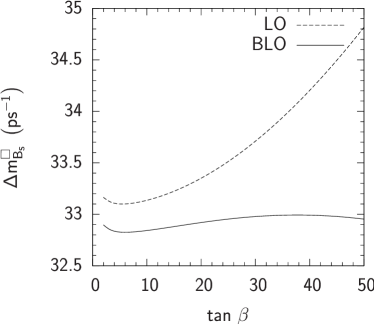
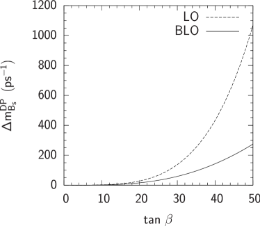
Figure 24: Contributions to $\Delta M_{B_{s}}$ vs. $\tan\beta$. The combined effect of box diagrams mediated by SUSY particles is shown in the left panel whilst the right panel shows the double penguin contribution. The soft sector is parameterised as follows: $m_{\widetilde{q}}=500\,\mbox{GeV}$, $A_{t}=-m_{\widetilde{q}}$, $m_{\widetilde{g}}=\sqrt{2}m_{\widetilde{q}}$, $\mu=m_{\widetilde{q}}$ and $m_{A}=300\,\mbox{GeV}$. The flavour violating parameters are $\delta_{LL}^{d}=\delta_{RR}^{d}=0.1$.

The panel on the left of Fig. 24 shows the $\tan\beta$ dependence of the contributions to $\Delta M_{B_{s}}$ arising from box diagrams mediated by SUSY particles. The main difference between the two curves at low $\tan\beta$, originates from the use of the NLO anomalous dimension matrix to run the BLO calculation from the SUSY matching scale to the electroweak matching scale. At large $\tan\beta$ the interference between the dominant gluino contribution and the BLO corrections to the chargino and neutralino contributions acts to reduce the overall contribution to $\Delta M_{B_{s}}$ further. As is apparent from plot however, the overall correction tends to be only of the order of five to ten percent.

The double penguin contributions are depicted on the panel on the right of Fig. 24. Here we see a rather more dramatic difference between LO and BLO calculations and at large $\tan\beta$ it is possible that BLO corrections can lead to a reduction of LO effects by up to a factor of three.

Let us briefly comment on which values of $\tan\beta$ should analyses, that typically only feature LO matching conditions for the gluino contributions to $\bar{B}_{s}-B_{s}$ mixing, include the double Higgs penguin contribution. As is evident from Fig. 24, the double penguin contribution completely dominates the behaviour of $\Delta M_{B_{s}}$ at large $\tan\beta$ and can become as important as the LO result for $\tan\beta$ as low as 20. We have checked that a similar situation arises for non–zero LR and RL insertions.

With these results in mind let us consider the combined effect of all the beyond Standard Model corrections in the large $\tan\beta$ regime.

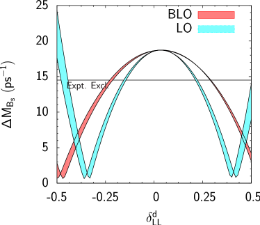
Figure 25: The dependence of $\Delta M_{B_{s}}$ on $\delta_{XY}^{d}$ for the same parameters as Fig. 22.

The dependence of $\Delta M_{B_{s}}$ on each of the flavour violating parameters is illustrated in Fig. 25. In the top left panel corresponding to the insertion $\delta_{LL}^{d}$ one can see a largely quadratic dependence on the insertion, in agreement with the analytic result (142). The graph is not centred on $\delta_{LL}^{d}=0$ as, in a similar manner to the $\bar{B}_{s}\to\mu^{+}\mu^{-}$ graph in Fig. 22, the MFV and GFM contributions to the neutral Higgs vertex approximately cancel for $\delta_{LL}^{d}\sim 0.08$. Turning to the top right panel, depicting the dependence of $\Delta M_{B_{s}}$ on $\delta_{LR}^{d}$, we can see that the overall effect on $\Delta M_{B_{s}}$ is rather slight, for small $\delta_{LR}^{d}$ the effect is mainly linear as $\delta_{LR}^{d}$ only contributes to the left–handed vertex that appears in (137). It is therefore necessary for the other penguin to be mediated by chargino exchange (143). For larger values of $\delta_{LR}^{d}$, contributions to $C_{1}^{SLL}$, as well as SUSY box diagrams, lead to a quadratic dependence on the insertion to emerge, however, once again, the corrections are rather small.

The bottom two panels depict the larger effects induced in the $\delta_{RL}^{d}$ and $\delta_{RR}^{d}$ sectors. The linear dependence of the contributions is due once again to one Higgs penguin being mediated by chargino exchange and the other by gluino exchange. The only alteration to this behaviour arises for very large $\delta_{RR}^{d}$ ($\sim 0.4$) where the gluino mediated contributions to the left–handed Higgs coupling, that are suppressed by a factor of $m_{s}$, can become important and interfere with the chargino contribution. Finally, let us once again point out the large differences between the LO and BLO calculations featured in all four plots. For $\delta_{LL}^{d}$ and $\delta_{RR}^{d}$ we see the characteristic suppression of LO effects that arise from the factors of $\left(1+\epsilon_{3}\tan\beta\right)$ and $\left(1+\epsilon_{s}\tan\beta\right)$ that appear in (138)–(146). These typically lead to reductions proportional to factors of two or three, if $\mu>0$. In a similar manner to the decay $\bar{B}_{s}\to\mu^{+}\mu^{-}$, a dependence on the insertions $\delta_{LR}^{d}$ and $\delta_{RL}^{d}$, which is absent at LO, reappears when BLO corrections are taken into account [17].

Before ending this section let us briefly discuss the correlation between $\bar{B}_{s}\to\mu^{+}\mu^{-}$ and $\Delta M_{B_{s}}$ at large $\tan\beta$. As was pointed out earlier in this subsection, the double Higgs penguin tends to completely dominate the contributions that arise from new physics in the large $\tan\beta$ regime. It is therefore natural to expect a degree of correlation with the decay $\bar{B}_{s}\to\mu^{+}\mu^{-}$, that is also dependent on the neutral Higgs penguin when $\tan\beta$ is large. Such a situation is illustrated by the scatter plots shown in Fig. 26.

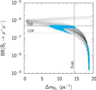
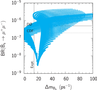
Figure 26: Scatter plots showing the correlation between $\Delta M_{B_{s}}$ and BR$(\bar{B}_{s}\to\mu^{+}\mu^{-})$. In the panel to the left $\delta_{LL}^{d}$ is varied over the range $[-0.8,0.8]$ whilst in the panel to the right the insertion $\delta_{RR}^{d}$ is varied over the same range of values. In both plots $m_{\widetilde{q}}$ is varied over the range $[500,1500]\,\mbox{GeV}$. The remaining parameters describing the SUSY sector are as follows: $\mu=500\,\mbox{GeV}$, $m_{A}=500\,\mbox{GeV}$, $A_{u}=-500\,\mbox{GeV}$ and $m_{\widetilde{g}}=1\,\mbox{TeV}$, $\tan\beta=40$. The published DØ and the preliminary CDF bounds for the decay $\bar{B}_{s}\to\mu^{+}\mu^{-}$ are shown, as well as the lower limit for $\Delta M_{B_{s}}$. Points compatible with $\bar{B}\to X_{s}\gamma$ are highlighted by light blue (light grey) squares.

Here we see in both panels that a large correlation exists between each process. The panel on the left (where only the LL insertion is varied) features only one branch as the double Higgs penguin in this case tends to only lead to a reduction in $\Delta M_{B_{s}}$. Varying the RR insertion can lead to reductions or enhancements of $\Delta M_{B_{s}}$ thanks to the linear dependence on the insertion exhibited in the matching condition given in (144). This effect leads to two distinct branches being visible in the right panel of Fig. 26.

7.4 Radiative Corrections to the CKM Matrix

It was mentioned briefly in subsection 3.4 that the rotation from the bare to the physical SCKM basis can induce large contributions to the bare CKM matrix $K^{(0)}$ [21]. One particularly interesting consequence of this is that the CKM matrix elements $K_{ts}$ and $K_{cb}$ could be generated radiatively via GFM effects [16]. Such a situation is illustrated in Fig. 27.

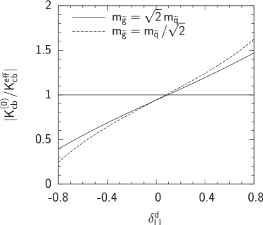
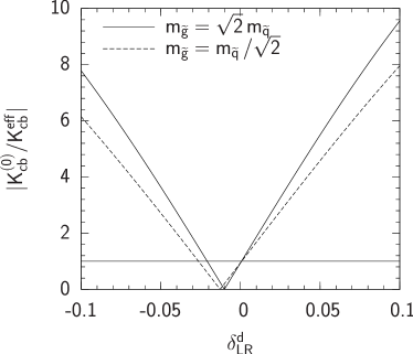
Figure 27: The ratio $K_{cb}^{(0)}/K^{\rm eff}_{cb}$ vs. $\delta_{LL}^{d}$ (the panel on the left) and $\delta_{LR}^{d}$ (the panel on the right). The soft sector is parameterised as follows: $\tan\beta=40$, $m_{\widetilde{q}}=1\,\mbox{TeV}$, $\mu=500\,\mbox{GeV}$, $m_{A}=500\,\mbox{GeV}$ and $A_{t}=-1\,\mbox{TeV}$. Solid and dashed lines denote $m_{\widetilde{g}}=\sqrt{2}\,m_{\widetilde{g}}$ and $m_{\widetilde{g}}=m_{\widetilde{q}}\,/\sqrt{2}$ respectively.

From both plots it is evident that $K_{cb}^{(0)}$ (and similarly $K_{ts}^{(0)}$) can receive significant corrections due to the presence of GFM in the squark sector. In the LR sector in particular, radiative generation of the entire matrix element can typically occur for $\delta_{LR}^{d}\sim-0.01$. One could imagine the scenario where corrections to the remaining matrix elements might induce similar effects and lead the CKM matrix to be fully diagonal before SUSY threshold corrections are taken into account.

From the top–right panel in Fig. 22 it is also apparent that, due to a cancellation between the chargino and gluino corrections to neutral Higgs vertex, the branching ratio of the decay $\bar{B}_{s}\to\mu^{+}\mu^{-}$ also tends to approach SM like values for negative $\delta_{LR}^{d}$. The minima of the two curves however tend not to coincide unless $\epsilon_{Y}Y_{t}^{2}\sim-\epsilon_{s}$ (this typically only occurs if $A_{t}$ is rather large and negative).

8 Summary

We have presented here the first complete analysis that includes the resummation of all $\tan\beta$ enhanced BLO effects in SUSY with GFM that contribute to the processes $\bar{B}\to X_{s}\gamma$, $\bar{B}_{s}\to\mu^{+}\mu^{-}$ and $\bar{B}_{s}-B_{s}$ mixing. We have derived analytic expressions applicable in general and in the MIA. As such, they match the precision of similar calculations performed in the context of MFV. We have provided a recipe for including BLO effects into LO expressions.

We have found that BLO effects in GFM can be large. In particular, we have more fully analysed the focusing effect that was initially pointed out in [15, 16] in the case of $\bar{B}\to X_{s}\gamma$ and next shown to also exist in the other two processes [17]. In the phenomenologically interesting case of large $\tan\beta$ and $\mu>0$ the focusing effect often leads to a significant relaxation of experimental bounds on the soft mass mixings.

Finally, we have examined radiative corrections to the CKM entries. These can be large, or even dominant, due to large LR mixings. We have pointed out a possible, although apparently accidental, correlation with the processes analysed here.

The method presented here is rather general and can readily be extended to include CP violating contributions, here BLO corrections can carry additional phases and lead to potentially large deviations from LO calculations. One might also consider the process $\bar{B}\to X_{s}l^{+}l^{-}$, where the BLO corrections to the Wilson coefficients $C_{7}$ and $C_{8}$ (and their primed counterparts) may also play a large rôle. Another possible application would be to include the $\bar{B}_{d}-B_{d}$ mixing system where, at large $\tan\beta$, one can expect strict bounds the insertions $\left(\delta_{RR}^{d}\right)_{13}$ and $\left(\delta_{RL}^{d}\right)_{13}$ due to contributions to $\Delta M_{B_{d}}$ unsuppressed by $m_{d}$.

The formalism presented here can be applied to data from present and future B–factories and hadron colliders in constraining mass insertions and, eventually, in extracting information on an emerging pattern of flavour violation in the squark sector [78].

Appendix A Loop Functions

A.1 The Functions $H_{i}$

The loop functions $H_{i}$ that appear throughout the text are given by

$$H_{2}(x_{1},x_{2})= \frac{x_{1}\log x_{1}}{\left(1-x_{1}\right)\left(x_{1}-x_{2}\right)}+\frac{x_{2}\log x_{2}}{\left(1-x_{2}\right)\left(x_{2}-x_{1}\right)},$$ (150)

$$H_{3}(x_{1},x_{2},x_{3})= \frac{H_{2}(x_{1},x_{2})-H_{2}(x_{1},x_{3})}{x_{2}-x_{3}},$$ (151)

$$H_{4}(x_{1},x_{2},x_{3},x_{4})= \frac{H_{3}(x_{1},x_{2},x_{3})-H_{3}(x_{1},x_{2},x_{4})}{x_{3}-x_{4}}.$$ (152)

In the limit of degenerate arguments the functions become

$$H_{2}\left(1,1\right) =-\frac{1}{2}, H_{3}\left(1,1,1\right) =\frac{1}{6}, H_{4}\left(1,1,1,1\right) =-\frac{1}{12}.$$ (153)

A.2 $\bar{B}\to X_{s}\gamma$

The loop functions $F_{7,8}^{(2)}\left(x\right)$ that appear in the charged Higgs matching conditions (89)–(91) are

$$F_{7}^{(2)}\left(x\right) =\frac{x\left(3-5x\right)}{12\left(x-1\right)^{2}}+\frac{x\left(3x-2\right)}{6\left(x-1\right)^{3}}\log x,$$

$$F_{8}^{(2)}\left(x\right) =\frac{x\left(3-x\right)}{4\left(x-1\right)^{2}}-\frac{x}{2\left(x-1\right)^{3}}\log x.$$

The functions $H_{i}^{[7,8]}\left(x\right)$ that appear in section 4.2 are given by the following expressions. The chargino contribution features the functions

$$H_{1}^{[7]}\left(x\right) =\frac{-3x^{2}+2x}{6\left(1-x\right)^{4}}\log x+\frac{-8x^{2}-5x+7}{36\left(1-x\right)^{3}},$$

$$H_{1}^{[8]}\left(x\right) =\frac{x}{2\left(1-x\right)^{4}}\log x+\frac{-x^{2}+5x+2}{12\left(1-x\right)^{3}},$$

$$H_{2}^{[7]}\left(x\right) =\frac{-3x^{2}+2x}{3\left(1-x\right)^{3}}\log x+\frac{-5x^{2}+3x}{6\left(1-x\right)^{2}},$$

$$H_{2}^{[8]}\left(x\right) =\frac{x}{\left(1-x\right)^{3}}\log x+\frac{-x^{2}+3x}{2\left(1-x\right)^{2}}.$$

The functions relevant to the neutralino contribution are given by

$$H_{3}^{[7]}\left(x\right) =-\frac{1}{3}H_{1}^{[8]}\left(x\right), H_{3}^{[8]}\left(x\right) =H_{1}^{[8]}\left(x\right),$$

$$H_{4}^{[7]}\left(x\right) =-\frac{1}{3}\left(H_{2}^{[8]}\left(x\right)+\frac{1}{2}\right), H_{4}^{[8]}\left(x\right) =H_{2}^{[8]}\left(x\right)+\frac{1}{2}.$$

The functions relevant to the gluino contribution are

$$H_{5}^{[7]}\left(x\right) =-\frac{1}{3}H_{1}^{[8]}\left(x\right) H_{5}^{[8]}\left(x\right) =\frac{9x^{2}-x}{16\left(1-x\right)^{4}}\log x+\frac{19x^{2}+40x-11}{96\left(1-x\right)^{3}},$$

$$H_{6}^{[7]}\left(x\right) =-\frac{1}{3}\left(H_{2}^{[8]}\left(x\right)+\frac{1}{2}\right), H_{6}^{[8]}\left(x\right) =\frac{9x^{2}-x}{8\left(1-x\right)^{3}}\log x+\frac{13x-5}{8\left(1-x\right)^{2}}.$$

The loop functions $I_{i}^{[7,8]}\left(x\right)$ and $J_{i}^{[7,8]}\left(x\right)$ that appear at higher orders in the MIA are related to the functions $H_{i}^{[7,8]}\left(x\right)$ via the relations

$$I_{i}^{[7,8]}\left(x\right) =\frac{d}{dx}H_{i}^{[7,8]}\left(x\right), J_{i}^{[7,8]}\left(x\right) =\frac{d^{2}}{dx^{2}}H_{i}^{[7,8]}\left(x\right).$$

A.3 $\bar{B}_{s}\to\mu^{+}\mu^{-}$

The function that appears in (120) is given by

$$f_{Z}\left(x\right)=\frac{x}{4\left(x-1\right)^{4}}\log x+\frac{\left(x^{3}-6x^{2}+3x+2\right)}{24\left(x-1\right)^{4}}.$$

A.4 $\bar{B}_{s}-B_{s}$

The functions that appear the gluino matching condition (147) are given by

$$f_{\widetilde{g}}^{[1]}\left(x\right)= \frac{x^{2}\left(x+3\right)}{\left(x-1\right)^{5}}\log x+\frac{(-17x^{3}+9x^{2}+9x-1)}{6\left(x-1\right)^{5}},$$

$$f_{\widetilde{g}}^{[2]}\left(x\right)= \frac{2x^{2}\left(x+1\right)}{\left(x-1\right)^{5}}\log x+\frac{(-x^{3}-9x^{2}+9x+1)x}{3\left(x-1\right)^{5}}.$$

A.5 Passarino–Veltman Functions

The Passarino–Veltman functions that appear in appendix D have the following form

$$B_{0}\left(x,y\right) =\eta-\log\frac{x}{\mu^{2}}+1+\frac{y}{x-y}\log\frac{y}{x},$$

$$B_{1}\left(x,y\right) =-\frac{1}{2}\eta+\frac{1}{2}\log\frac{x}{\mu^{2}}-\frac{1}{4}-\frac{x}{2\left(x-y\right)}+\frac{y^{2}-2xy}{2\left(x-y\right)^{2}}\log\frac{y}{x},$$

$$C_{0}\left(x,y,z\right) =\frac{y}{(x-y)(y-z)}\log\frac{y}{x}+\frac{z}{(x-z)(z-y)}\log\frac{z}{x},$$

$$C_{00}\left(x,y,z\right) =\frac{1}{4}\left(\eta+\frac{3}{2}-\log\frac{x}{\mu^{2}}+\frac{y^{2}}{(x-y)(y-z)}\log\frac{y}{x}+\frac{z^{2}}{(x-z)(z-y)}\log\frac{z}{x}\right),$$

where $\eta=\frac{2}{\epsilon}+\log 4\pi-\gamma_{E}$.

Appendix B Alternative forms for $\delta_{LR}^{d}$ and $\delta_{RL}^{d}$

As discussed in section 2, throughout this analysis we assume that the trilinear SUSY breaking terms are not proportional to the appropriate Yukawa coupling. To illustrate how our results are altered if we do make this assumption, let us consider a specific example with relevance to models with SUSY breaking mediated by either supergravity or gauge interactions [80]

$$m_{d,LR}^{2}=\tilde{A}_{d\,L}^{{\dagger}}m_{d}^{(0)}{}^{{\dagger}}+m_{d}^{(0)}{}^{{\dagger}}\tilde{A}_{d\,R}^{{\dagger}}.$$ (154)

The insertions $\delta_{LR}^{d}$ and $\delta_{RL}^{d}$ are therefore equal to

$$\left(\delta_{LR}^{d}\right)_{23}= \frac{\left(\tilde{A}_{d\,L}^{{\dagger}}m_{d}^{(0)}{}^{{\dagger}}\right)_{23}+\left(m_{d}^{(0)}{}^{{\dagger}}\tilde{A}_{d\,R}^{{\dagger}}\right)_{23}}{\sqrt{\left(m_{d,LL}^{2}\right)_{22}\left(m^{2}_{d,RR}\right)_{33}}}$$

$$\left(\delta_{RL}^{d}\right)_{23}= \frac{\left(\tilde{A}_{d\,R}m_{d}^{(0)}\right)_{23}+\left(m_{d}^{(0)}\tilde{A}_{d\,L}\right)_{23}}{\sqrt{\left(m_{d,LL}^{2}\right)_{33}\left(m^{2}_{d,RR}\right)_{22}}}$$ (155)

It should be noted that, in addition to the off–diagonal elements of the complex matrices $\tilde{A}_{d}^{L,R}$, there is a contribution proportional to the appropriate off–diagonal element of $m_{d}^{(0)}$. If we use the choice (154), one can redefine the insertions $\delta_{LR}^{d}$ and $\delta_{RL}^{d}$ (155) to be independent of the bare mass matrix in the following way (ignoring terms suppressed by the strange quark mass)

$$\left(\delta_{LR}^{d}\right)_{23}= \frac{m_{b}\left(\tilde{A}_{d\,L}^{{\dagger}}\right)_{23}}{\sqrt{\left(m_{d,LL}^{2}\right)_{22}\left(m^{2}_{d,RR}\right)_{33}}}, \left(\delta_{RL}^{d}\right)_{23}= \frac{m_{b}\left(\tilde{A}_{d\,R}\right)_{23}}{\sqrt{\left(m_{d,LL}^{2}\right)_{22}\left(m^{2}_{d,RR}\right)_{33}}}.$$

This definition is largely independent of BLO corrections and would correspond to a input value appropriate for the iterative procedure described in section 2.4. The effects due to the bare mass matrix then appear in two ways. The diagonal elements result in a factor of $1/\left(1+\epsilon_{3}\tan\beta\right)$ that accompanies each factor of $\delta_{LR}^{d}$ and $\delta_{RL}^{d}$. The off–diagonal elements, on the other hand, may be included in a similar manner to the off–diagonal elements of the $F$–terms that appear in the squark mass matrix by altering $\epsilon_{s}$ with a small ($\cot\beta$ suppressed) correction. The only exception to this rule concerns the corrected charged Higgs vertex, where one must perform the substitution

$$\delta_{LR}^{d}\to\delta_{LR}^{d}+\frac{\left(\tilde{A}_{d\,L}^{{\dagger}}\right)_{22}\left(m_{d}^{(0)}{}^{{\dagger}}\right)_{23}+\left(\tilde{A}_{d\,R}^{{\dagger}}\right)_{33}\left(m_{d}^{(0)}{}^{{\dagger}}\right)_{23}}{\sqrt{\left(m_{d,LL}^{2}\right)_{22}\left(m^{2}_{d,RR}\right)_{33}}}$$

in (58). In the limit of MFV ($\tilde{A}_{d\,L}=A_{0}$, $\tilde{A}_{d\,R}=0$) we reproduce the result presented in [14].

Appendix C Supersymmetric Vertices

Now let us present a complete list of supersymmetric vertices required for our calculation. Throughout this section $I,J=1,\dots,6$, $a,b=1,2$, $\alpha,\beta=1,\dots,4$ and finally $i,j=1,2,3$.

The coupling of the gluino to down quarks and squarks is given by

$$\mathcal{L}_{\widetilde{g}}= \;\tilde{d}_{J}^{\dagger}\left(\bar{g}\right)\left[\left(G_{d\,L}\right)_{Ji}P_{L}+\left(G_{d\,R}\right)_{Ji}P_{R}\right]\left(d\right)_{i},$$ (156)

where $\left(G_{d\,L}\right)_{Ji}$ and $\left(G_{d\,R}\right)_{Ji}$ are given by

$$\left(G_{d\,L}\right)_{Ji} =-\sqrt{2}g_{s}\left(\Gamma_{d\,L}\right)_{Ji}, \left(G_{d\,R}\right)_{Ji} =\sqrt{2}g_{s}\left(\Gamma_{d\,R}\right)_{Ji}$$ (157)

The couplings to up quarks and squarks may be obtained via the simple substitution $d\to u$.

The chargino coupling to down quarks and up squarks was discussed in section 2.3 whilst the coupling to up quarks and down squarks is given by

$$\left(C_{u\,L}\right)_{aJi}= -g_{2}U_{a1}\left(\Gamma_{d\,L}K^{{\dagger}}\right)_{Ji}+\frac{g_{2}}{\sqrt{2}m_{W}\cos\beta}U_{a2}\left(\Gamma_{d\,R}m_{d}^{(0)}K^{{\dagger}}\right)_{Ji}$$ (158)

$$\left(C_{u\,R}\right)_{aJi}= \frac{g_{2}}{\sqrt{2}m_{W}\sin\beta}V_{a2}\left(\Gamma_{d\,L}K^{{\dagger}}m_{u}^{(0)}{}^{\dagger}\right)_{Ji}$$ (159)

The neutralino couplings between down quarks and squarks are

$$\mathcal{L}_{\chi^{0}}= \;\tilde{d}_{J}^{\dagger}\left(\bar{\chi}^{0}\right)_{\alpha}\left[\left(N_{d\,L}\right)_{\alpha Ji}P_{L}+\left(N_{d\,R}\right)_{\alpha Ji}P_{R}\right]\left(d\right)_{i},$$ (160)

where $\left(N_{d\,L}\right)_{Ji\alpha}$ and $\left(N_{d\,R}\right)_{Ji\alpha}$ are given by

$$\left(N_{d\,L}\right)_{\alpha Ji}= -\frac{g_{2}}{\sqrt{2}}\left(\frac{1}{3}N_{\alpha 1}^{\ast}\tan\theta_{W}-N_{\alpha 2}^{\ast}\right)\left(\Gamma_{d\,L}\right)_{Ji}-\frac{g_{2}}{\sqrt{2}m_{W}\cos\beta}N_{\alpha 3}^{\ast}\left(\Gamma_{d\,R}m_{d}^{(0)}\right)_{Ji},$$ (161)

$$\left(N_{d\,R}\right)_{\alpha Ji}= -\frac{g_{2}\sqrt{2}\tan\theta_{W}}{3}N_{\alpha 1}\left(\Gamma_{d\,R}\right)_{Ji}-\frac{g_{2}}{\sqrt{2}m_{W}\cos\beta}N_{\alpha 3}\left(\Gamma_{d\,L}m_{d}^{(0)}{}^{\dagger}\right)_{Ji}.$$ (162)

The matrix $N$ diagonalises the neutralino mass matrix in the usual manner

$$N^{\ast}\mathcal{M}_{\chi^{0}}N^{{\dagger}}={\rm diag}\left(m_{\chi^{0}_{1}},\dots,m_{\chi^{0}_{4}}\right).$$ (163)

The couplings to up quarks and squarks are

$$\left(N_{u\,L}\right)_{\alpha Ji}= -\frac{g_{2}}{\sqrt{2}}\left(\frac{1}{3}N_{\alpha 1}^{\ast}\tan\theta_{W}+N_{\alpha 2}^{\ast}\right)\left(\Gamma_{d\,L}\right)_{Ji}-\frac{g_{2}}{\sqrt{2}m_{W}\sin\beta}N_{\alpha 4}^{\ast}\left(\Gamma_{u\,R}m_{u}^{(0)}\right)_{Ji},$$ (164)

$$\left(N_{u\,R}\right)_{\alpha Ji}= \frac{2\sqrt{2}g_{2}\tan\theta_{W}}{3}N_{\alpha 1}\left(\Gamma_{u\,R}\right)_{Ji}-\frac{g_{2}}{\sqrt{2}m_{W}\sin\beta}N_{\alpha 4}\left(\Gamma_{u\,L}m_{u}^{(0)}{}^{\dagger}\right)_{Ji}.$$ (165)

Let us now consider the couplings of the $W$ boson that appear in (185). The coupling to squarks is given by

$$\left(W_{\widetilde{d}}\right)_{IJ}=-\frac{g_{2}}{\sqrt{2}}\left(\Gamma_{u\,L}K\Gamma_{d\,L}^{{\dagger}}\right)_{IJ}.$$ (166)

The couplings to neutralinos and charginos are given by

$$\left(W_{\chi\,L}\right)_{a\alpha} =g_{2}\left(N_{\alpha 2}^{\ast}V_{a1}-\frac{1}{\sqrt{2}}N_{\alpha 4}^{\ast}V_{a2}\right) \left(W_{\chi\,R}\right)_{a\alpha} =g_{2}\left(N_{\alpha 2}U_{a1}+\frac{1}{\sqrt{2}}N_{\alpha 3}U_{a2}\right)$$ (167)

The couplings of the $Z$ boson to up and down squarks are given by

$$\left(Z_{\widetilde{d}}\right)_{IJ} =\frac{g_{2}}{2\cos\theta_{W}}\left(\Gamma_{d\,L}\Gamma_{d\,L}^{{\dagger}}-\frac{2}{3}\sin^{2}\theta_{W}\right)_{IJ},$$ (168)

$$\left(Z_{\widetilde{u}}\right)_{IJ} =-\frac{g_{2}}{2\cos\theta_{W}}\left(\Gamma_{u\,L}\Gamma_{u\,L}^{{\dagger}}-\frac{4}{3}\sin^{2}\theta_{W}\right)_{IJ}.$$ (169)

The couplings to neutralinos and charginos on the other hand are

$$\left(Z_{\chi^{-}\,L}\right)_{ab} =\frac{g_{2}}{2\cos\theta_{W}}\left[U_{a1}U_{b1}^{\ast}+\left(\cos^{2}\theta_{W}-\sin^{2}\theta_{W}\right)\delta_{ab}\right],$$ (170)

$$\left(Z_{\chi^{-}\,R}\right)_{ab} =\frac{g_{2}}{2\cos\theta_{W}}\left[V_{a1}V_{b1}^{\ast}+\left(\cos^{2}\theta_{W}-\sin^{2}\theta_{W}\right)\delta_{ab}\right],$$ (171)

$$\left(Z_{\chi^{0}\,L}\right)_{\alpha\beta} =\frac{g_{2}}{2\cos\theta_{W}}\left(N_{\alpha 4}N_{\beta 4}^{\ast}-N_{\alpha 3}N_{\beta 3}^{\ast}\right),$$ (172)

$$\left(Z_{\chi^{0}\,R}\right)_{\alpha\beta} =-\frac{g_{2}}{2\cos\theta_{W}}\left(N_{\alpha 4}^{\ast}N_{\beta 4}-N_{\alpha 3}^{\ast}N_{\beta 3}\right).$$ (173)

The coupling of the charged Higgs boson to squarks is given by

$$\left(C_{\widetilde{d}}^{S^{+}}\right)_{IJ}= -\frac{g_{2}m_{W}}{\sqrt{2}\sin\theta_{W}}\left(\cos\beta y_{(2)}^{S^{+}}+\sin\beta y_{(1)}^{S^{+}}\right)\left(\Gamma_{u\,L}K\Gamma_{d\,L}^{{\dagger}}\right)_{IJ}$$

$$+\frac{g_{2}}{\sqrt{2}m_{W}}\left[\frac{y_{(2)}^{S^{+}}}{\cos\beta}\left(\Gamma_{u\,L}Km_{d}^{(0)}{}^{{\dagger}}m_{d}^{(0)}\Gamma_{d\,L}^{{\dagger}}\right)_{IJ}+\frac{y_{(1)}^{S^{+}}}{\sin\beta}\left(\Gamma_{u\,L}m_{u}^{(0)}{}^{{\dagger}}m_{u}^{(0)}K\Gamma_{d\,L}^{{\dagger}}\right)_{IJ}\right]$$

$$+\frac{g_{2}\eta_{S^{+}}}{\sqrt{2}\cos\beta\sin\beta}\left(\Gamma_{u\,R}m_{u}^{(0)}Km_{d}^{(0)}{}^{{\dagger}}\Gamma_{d\,R}^{{\dagger}}\right)_{IJ}$$

$$+y_{(2)}^{S^{+}}\frac{g_{2}}{\sqrt{2}m_{W}\cos\beta}\left[\left(\Gamma_{u\,L}Km_{d,LR}\Gamma_{d\,R}^{{\dagger}}\right)_{IJ}+\mu^{\ast}\cot\beta\left(\Gamma_{u\,R}m_{u}^{(0)}K\Gamma_{d\,L}^{{\dagger}}\right)_{IJ}\right]$$

$$+y_{(1)}^{S^{+}}\frac{g_{2}}{\sqrt{2}m_{W}\sin\beta}\left[\left(\Gamma_{u\,R}m_{u,RL}K\Gamma_{d\,L}^{{\dagger}}\right)_{IJ}+\mu\tan\beta\left(\Gamma_{u\,L}Km_{d}^{(0)}{}^{{\dagger}}\Gamma_{d\,R}^{{\dagger}}\right)_{IJ}\right],$$ (174)

where $\eta_{S^{+}}=1,0$ The coupling of the charged Higgs to the chargino and neutralinos is given by

$$\left(C_{\chi\,L}^{S^{+}}\right)_{a\alpha}= \frac{g_{2}}{\cos\theta_{W}}y_{(2)}^{S^{+}}\left[\frac{1}{\sqrt{2}}U_{a2}\left(N_{\alpha 1}^{\ast}\sin\theta_{W}+N_{\alpha 2}^{\ast}\cos\theta_{W}\right)-U_{a1}N_{\alpha 3}^{\ast}\cos\theta_{W}\right],$$ (175)

$$\left(C_{\chi\,R}^{S^{+}}\right)_{a\alpha}= -\frac{g_{2}}{\cos\theta_{W}}y_{(1)}^{S^{+}}\left[\frac{1}{\sqrt{2}}V_{a2}\left(N_{\alpha 1}\sin\theta_{W}+N_{\alpha 2}\cos\theta_{W}\right)+V_{a1}N_{\alpha 4}\cos\theta_{W}\right].$$ (176)

The couplings of the neutral Higgs bosons to squarks are

$$\left(S_{\widetilde{d}}^{S^{0}}\right)_{IJ}= \eta_{S^{0}}\bigg{\{}\frac{g_{2}}{3}\tan^{2}\theta_{W}m_{W}\left(\cos\beta x_{(1)}^{S^{0}}-\sin\beta x_{(2)}^{S^{0}}\right)\left(1+\frac{3-4\sin^{2}\theta_{W}}{2\sin^{2}\theta_{W}}\Gamma_{d\,L}\Gamma_{d\,L}^{{\dagger}}\right)_{IJ}$$

$$-\frac{g_{2}}{m_{W}\cos\beta}x_{(1)}^{S^{0}}\left[\left(\Gamma_{d\,L}m_{d}^{(0)}{}^{{\dagger}}m_{d}^{(0)}\Gamma_{d\,L}^{{\dagger}}\right)_{IJ}+\left(\Gamma_{d\,R}m_{d}^{(0)}m_{d}^{(0)}{}^{{\dagger}}\Gamma_{d\,R}^{{\dagger}}\right)_{IJ}\right]\bigg{\}}$$

$$-\frac{g_{2}}{2m_{W}\cos\beta}\bigg{[}\left(\Gamma_{d\,R}m_{d,RL}\Gamma_{d\,L}^{{\dagger}}\right)_{IJ}x_{(1)}^{S^{0}}+\left(\Gamma_{d\,L}m_{d,LR}\Gamma_{d\,R}^{{\dagger}}\right)_{IJ}x_{(1)}^{S^{0}\ast}$$

$$-\mu\left(\Gamma_{d\,L}m_{d}^{(0)}{}^{{\dagger}}\Gamma_{d\,R}^{{\dagger}}\right)_{IJ}x_{(2)}^{S^{0}}-\mu^{\ast}\left(\Gamma_{d\,R}m_{d}^{(0)}\Gamma_{d\,L}^{{\dagger}}\right)_{IJ}x_{(2)}^{S^{0}\ast}\bigg{]},$$ (177)

$$\left(S_{\widetilde{u}}^{S^{0}}\right)_{IJ}= \eta_{S^{0}}\bigg{\{}-\frac{2g_{2}}{3}\tan^{2}\theta_{W}m_{W}\left(\cos\beta x_{(1)}^{S^{0}}-\sin\beta x_{(2)}^{S^{0}}\right)\left(1+\frac{3-8\sin^{2}\theta_{W}}{4\sin^{2}\theta_{W}}\Gamma_{u\,L}\Gamma_{u\,L}^{{\dagger}}\right)_{IJ}$$

$$-\frac{g_{2}}{m_{W}\sin\beta}x_{(2)}^{S^{0}}\left[\left(\Gamma_{u\,L}m_{u}^{(0)}{}^{{\dagger}}m_{u}^{(0)}\Gamma_{u\,L}^{{\dagger}}\right)_{IJ}+\left(\Gamma_{u\,R}m_{u}^{(0)}m_{u}^{(0)}{}^{{\dagger}}\Gamma_{u\,R}^{{\dagger}}\right)_{IJ}\right]\bigg{\}}$$

$$-\frac{g_{2}}{2m_{W}\sin\beta}\bigg{[}\left(\Gamma_{u\,R}m_{u,RL}\Gamma_{u\,L}^{{\dagger}}\right)_{IJ}x_{(2)}^{S^{0}}+\left(\Gamma_{u\,L}m_{u,LR}\Gamma_{u\,R}^{{\dagger}}\right)_{IJ}x_{(2)}^{S^{0}\ast}$$

$$-\mu\left(\Gamma_{u\,L}m_{u}^{(0)}{}^{{\dagger}}\Gamma_{u\,R}^{{\dagger}}\right)_{IJ}x_{(1)}^{S^{0}}-\mu^{\ast}\left(\Gamma_{u\,R}m_{u}^{(0)}\Gamma_{u\,L}^{{\dagger}}\right)_{IJ}x_{(1)}^{S^{0}\ast}\bigg{]},$$ (178)

where $\eta_{S^{0}}=1,1,0,0$ and $x_{(2)}^{S^{0}}=\sin\alpha,\cos\alpha,i\cos\beta,i\sin\beta$

The couplings of the bosons to charginos and neutralinos are

$$\left(S_{\chi^{-}L}\right)_{ab}= -\frac{g_{2}}{\sqrt{2}}\left(x_{(1)}^{S^{0}\ast}U_{a2}V_{b1}^{\ast}+x_{(2)}^{S^{0}\ast}U_{a1}V_{b2}^{\ast}\right),$$ (179)

$$\left(S_{\chi^{-}R}\right)_{ab}= -\frac{g_{2}}{\sqrt{2}}\left(x_{(1)}^{S^{0}}U_{a2}^{\ast}V_{b1}+x_{(2)}^{S^{0}}U_{a1}^{\ast}V_{b2}\right),$$ (180)

$$\left(S_{\chi^{0}\,L}\right)_{\alpha\beta}= \frac{g_{2}}{2\cos\theta_{W}}\bigg{[}\left(x_{(1)}^{S^{0}\ast}N_{\alpha 3}^{\ast}-x_{(2)}^{S^{0}\ast}N_{\alpha 4}^{\ast}\right)\left(N_{\beta 1}^{\ast}\sin\theta_{W}-N_{\beta 2}^{\ast}\cos\theta_{W}\right)$$

$$+\left(x_{(1)}^{S^{0}\ast}N_{\beta 3}^{\ast}-x_{(2)}^{S^{0}\ast}N_{\beta 4}^{\ast}\right)\left(N_{\alpha 1}^{\ast}\sin\theta_{W}-N_{\alpha 2}^{\ast}\cos\theta_{W}\right)\bigg{]},$$ (181)

$$\left(S_{\chi^{0}\,R}\right)_{\alpha\beta}= \frac{g_{2}}{2\cos\theta_{W}}\bigg{[}\left(x_{(1)}^{S^{0}}N_{\alpha 3}-x_{(2)}^{S^{0}}N_{\alpha 4}\right)\left(N_{\beta 1}\sin\theta_{W}-N_{\beta 2}\cos\theta_{W}\right)$$

$$+\left(x_{(1)}^{S^{0}}N_{\beta 3}-x_{(2)}^{S^{0}}N_{\beta 4}\right)\left(N_{\alpha 1}\sin\theta_{W}-N_{\alpha 2}\cos\theta_{W}\right)\bigg{]}.$$ (182)

Appendix D Corrected Vertices

Let us now present the full analytic expressions used in our numerical analysis. A number of the corrections given in this section are divergent and should be renormalized appropriately. However, we have checked that numerically these terms are negligible compared to the $\tan\beta$ enhanced corrections discussed in 3 and tend to play only a minor rôle. Throughout this section $i,j=1,2,3$, $I,J=1,\dots,6$, $a,b=1,2$, $\alpha,\beta=1,\dots,4$, $S^{+}=H^{+},G^{+}$ and $S^{0}=H^{0},h^{0},A^{0},G^{0}$. Repeated indices that appear in the expressions below should be summed over. We have checked are results with those that appear in [14] and find that, once one takes into account the different form of Passarino–Veltman functions we adopt our results agree.

The self–energies that appear in the corrected vertices presented in section 2.2 as well as the expression for $\delta m_{d}$ are given by

$$\left(\Sigma^{d}_{m\,L}\right)_{ij}= -\frac{1}{16\pi^{2}}\bigg{[}m_{\widetilde{g}}\left(G_{d\,R}^{\ast}\right)_{Ii}\left(G_{d\,L}\right)_{Ij}C_{2}\left(3\right)B_{0}\left(m_{\widetilde{g}}^{2},m_{\widetilde{d}_{I}}^{2}\right)$$

$$+m_{\chi^{-}_{a}}\left(C_{d\,R}^{\ast}\right)_{aIi}\left(C_{d\,L}\right)_{aIj}B_{0}\left(m_{\chi^{-}_{a}}^{2},m_{\widetilde{u}_{I}}^{2}\right)$$

$$+m_{\chi^{0}_{\alpha}}\left(N_{d\,R}^{\ast}\right)_{\alpha Ii}\left(N_{d\,L}\right)_{\alpha Ij}B_{0}\left(m_{\chi^{0}_{\alpha}}^{2},m_{\widetilde{d}_{I}}^{2}\right)\bigg{]},$$ (183)

$$\left(\Sigma^{d}_{v\,L}\right)_{ij}= \frac{1}{16\pi^{2}}\bigg{[}\left(G_{d\,L}^{\ast}\right)_{Ii}\left(G_{d\,L}\right)_{Ij}C_{2}\left(3\right)B_{1}\left(m_{\widetilde{g}}^{2},m_{\widetilde{d}_{I}}^{2}\right)$$

$$+\left(C_{d\,L}^{\ast}\right)_{aIi}\left(C_{d\,L}\right)_{aIj}B_{1}\left(m_{\chi^{-}_{a}}^{2},m_{\widetilde{u}_{I}}^{2}\right)$$

$$+\left(N_{d\,L}^{\ast}\right)_{\alpha Ii}\left(N_{d\,L}\right)_{\alpha Ij}B_{1}\left(m_{\chi^{0}_{\alpha}}^{2},m_{\widetilde{d}_{I}}^{2}\right)\bigg{]}.$$ (184)

The various supersymmetric couplings that appear in the above expressions are given in appendix C whilst the Passarino–Veltman functions are defined in appendix A.5. $\Sigma^{d}_{v\,R}$ can be obtained by substituting $L$ with $R$ in (184) the up quark self–energy corrections can be obtained by substituting $u\leftrightarrow d$.

The correction $\Delta C_{L}^{W}$ that appears in (26) is given by

$$\left(\Delta C_{L}^{W}\right)_{ij}= \frac{1}{16\pi^{2}}\bigg{\{}2C_{2}\left(3\right)\left(W_{\widetilde{d}}\right)_{IJ}\left(G_{u\,L}^{\ast}\right)_{Ii}\left(G_{d\,L}\right)_{Jj}C_{00}\left(m_{\widetilde{g}}^{2},m_{\widetilde{d}_{J}}^{2},m_{\widetilde{u}_{I}}^{2}\right)$$

$$+2\left(W_{\widetilde{d}}\right)_{IJ}\left(N_{u\,L}^{\ast}\right)_{\alpha Ii}\left(N_{d\,L}\right)_{\alpha Jj}C_{00}\left(m_{\chi^{0}_{\alpha}}^{2},m_{\widetilde{d}_{J}}^{2},m_{\widetilde{u}_{I}}^{2}\right)$$

$$+m_{\chi^{0}_{\alpha}}m_{\chi^{-}_{a}}\left(W_{\chi\,R}\right)_{a\alpha}\left(N_{u\,L}^{\ast}\right)_{\alpha Ii}\left(C_{d\,L}\right)_{aIj}C_{0}\left(m_{\chi^{0}_{\alpha}}^{2},m_{\chi^{-}_{a}}^{2},m_{\widetilde{u}_{I}}^{2}\right)$$

$$-m_{\chi^{0}_{\alpha}}m_{\chi^{-}_{a}}\left(W_{\chi\,L}\right)_{a\alpha}\left(C_{u\,L}^{\ast}\right)_{aJi}\left(N_{d\,L}\right)_{\alpha Jj}C_{0}\left(m_{\chi^{0}_{\alpha}}^{2},m_{\chi^{-}_{a}}^{2},m_{\widetilde{d}_{J}}^{2}\right)$$

$$-2\left(W_{\chi\,L}\right)_{a\alpha}\left(N_{u\,L}^{\ast}\right)_{\alpha Ii}\left(C_{d\,L}\right)_{aIj}\left[C_{00}\left(m_{\chi^{0}_{\alpha}}^{2},m_{\chi^{-}_{a}}^{2},m_{\widetilde{u}_{I}}^{2}\right)-\frac{1}{4}\right]$$

$$+2\left(W_{\chi\,R}\right)_{a\alpha}\left(C_{u\,L}^{\ast}\right)_{aJi}\left(N_{d\,L}\right)_{\alpha Jj}\left[C_{00}\left(m_{\chi^{0}_{\alpha}}^{2},m_{\chi^{-}_{a}}^{2},m_{\widetilde{d}_{J}}^{2}\right)-\frac{1}{4}\right]\bigg{\}}.$$ (185)

$\Delta C_{R}^{W}$ can be obtained by the simple substitution $L\leftrightarrow R$. The correction to the left handed coupling of the $Z$–boson (29) is given by

$$\left(\Delta C_{L}^{Z}\right)_{ij}= \frac{1}{16\pi^{2}}\bigg{\{}2C_{2}\left(3\right)\left(Z_{\widetilde{d}}\right)_{IJ}\left(G_{d\,L}^{\ast}\right)_{Ii}\left(G_{d\,L}\right)_{Jj}C_{00}\left(m_{\widetilde{g}}^{2},m_{\widetilde{d}_{I}}^{2},m_{\widetilde{d}_{J}}^{2}\right)$$

$$+2\left(Z_{\widetilde{d}}\right)_{IJ}\left(N_{d\,L}^{\ast}\right)_{\alpha Ii}\left(N_{d\,L}\right)_{\alpha Jj}C_{00}\left(m_{\chi^{0}_{\alpha}}^{2},m_{\widetilde{d}_{I}}^{2},m_{\widetilde{d}_{J}}^{2}\right)$$

$$+2\left(Z_{\widetilde{u}}\right)_{IJ}\left(C_{d\,L}^{\ast}\right)_{aIi}\left(C_{d\,L}\right)_{aJj}C_{00}\left(m_{\chi^{-}_{a}}^{2},m_{\widetilde{u}_{I}}^{2},m_{\widetilde{u}_{J}}^{2}\right)$$

$$-m_{\chi^{-}_{a}}m_{\chi^{-}_{b}}\left(Z_{\chi^{-}\,L}\right)_{ab}\left(C_{d\,L}^{\ast}\right)_{bIi}\left(C_{d\,L}\right)_{aIj}C_{0}\left(m_{\chi^{-}_{a}}^{2},m_{\chi^{-}_{b}}^{2},m_{\widetilde{u}_{I}}^{2}\right)$$

$$-m_{\chi^{0}_{\alpha}}m_{\chi^{0}_{\beta}}\left(Z_{\chi^{0}\,L}\right)_{\alpha\beta}\left(N_{d\,L}^{\ast}\right)_{\beta Ji}\left(N_{d\,L}\right)_{\alpha Jj}C_{0}\left(m_{\chi^{0}_{\alpha}}^{2},m_{\chi^{0}_{\beta}}^{2},m_{\widetilde{d}_{J}}^{2}\right)$$

$$+2\left(Z_{\chi^{-}\,R}\right)_{ab}\left(C_{d\,L}^{\ast}\right)_{bIi}\left(C_{d\,L}\right)_{aIj}\left[C_{00}\left(m_{\chi^{-}_{a}}^{2},m_{\chi^{-}_{b}}^{2},m_{\widetilde{u}_{I}}^{2}\right)-\frac{1}{4}\right]$$

$$+2\left(Z_{\chi^{0}\,R}\right)_{\alpha\beta}\left(N_{d\,L}^{\ast}\right)_{\beta Ji}\left(N_{d\,L}\right)_{\alpha Jj}\left[C_{00}\left(m_{\chi^{0}_{\alpha}}^{2},m_{\chi^{0}_{\beta}}^{2},m_{\widetilde{d}_{J}}^{2}\right)-\frac{1}{4}\right]\bigg{\}}.$$ (186)

$\Delta C_{R}^{Z}$ may be obtained in a similar manner to $\Delta C_{R}^{W}$.

Turning to the Higgs sector the vertex correction $\Delta C_{L}^{S^{+}}$ is given by

$$\left(\Delta C_{L}^{S^{+}}\right)_{ij}= -\frac{1}{16\pi^{2}}\bigg{\{}C_{2}\left(3\right)m_{\widetilde{g}}\left(C_{\widetilde{d}}^{S^{+}}\right)_{IJ}\left(G_{u\,R}^{\ast}\right)_{Ii}\left(G_{d\,L}\right)_{Jj}C_{0}\left(m_{\widetilde{g}}^{2},m_{\widetilde{d}_{J}}^{2},m_{\widetilde{u}_{I}}^{2}\right)$$

$$+m_{\chi^{0}_{\alpha}}\left(C_{\widetilde{d}}^{S^{+}}\right)_{IJ}\left(N_{u\,R}^{\ast}\right)_{\alpha Ii}\left(N_{d\,L}\right)_{\alpha Jj}C_{0}\left(m_{\chi^{0}_{\alpha}}^{2},m_{\widetilde{d}_{J}}^{2},m_{\widetilde{u}_{I}}^{2}\right)$$

$$+m_{\chi^{0}_{\alpha}}m_{\chi^{-}_{a}}\left(C_{\chi L}^{S^{+}}\right)_{a\alpha}\left(N_{u\,R}^{\ast}\right)_{\alpha Ii}\left(C_{d\,L}\right)_{aIj}C_{0}\left(m_{\chi^{0}_{\alpha}}^{2},m_{\chi^{-}_{a}}^{2},m_{\widetilde{u}_{I}}^{2}\right)$$

$$+m_{\chi^{-}_{a}}m_{\chi^{0}_{\alpha}}\left(C_{\chi L}^{S^{+}}\right)_{a\alpha}\left(C_{u\,R}^{\ast}\right)_{aJi}\left(N_{d\,L}\right)_{\alpha Jj}C_{0}\left(m_{\chi^{-}_{a}}^{2},m_{\chi^{0}_{\alpha}}^{2},m_{\widetilde{d}_{J}}^{2}\right)$$

$$+4\left(C_{\chi R}^{S^{+}}\right)_{a\alpha}\left(N_{u\,R}^{\ast}\right)_{\alpha Ii}\left(C_{d\,L}\right)_{aIj}\left[C_{00}\left(m_{\chi^{0}_{\alpha}}^{2},m_{\chi^{-}_{a}}^{2},m_{\widetilde{u}_{I}}^{2}\right)-\frac{1}{8}\right]$$

$$+4\left(C_{\chi R}^{S^{+}}\right)_{a\alpha}\left(C_{u\,R}^{\ast}\right)_{aJi}\left(N_{d\,L}\right)_{\alpha Jj}\left[C_{00}\left(m_{\chi^{-}_{a}}^{2},m_{\chi^{0}_{\alpha}}^{2},m_{\widetilde{d}_{J}}^{2}\right)-\frac{1}{8}\right]\bigg{\}}.$$ (187)

$\Delta C_{R}^{S^{+}}$ may be obtained via the substitution $L\leftrightarrow R$. Finally the corrections to the neutral Higgs vertex may be written

$$\left(\Delta C_{L}^{S^{0}}\right)_{ij}= -\frac{1}{16\pi^{2}}\bigg{\{}C_{2}\left(3\right)m_{\widetilde{g}}\left(S_{\widetilde{d}}^{S^{0}}\right)_{IJ}\left(G_{d\,R}^{\ast}\right)_{Ii}\left(G_{d\,L}\right)_{Jj}C_{0}\left(m_{\widetilde{g}}^{2},m_{\widetilde{d}_{I}}^{2},m_{\widetilde{d}_{J}}^{2}\right)$$

$$+m_{\chi^{0}_{\alpha}}\left(S_{\widetilde{d}}^{S^{0}}\right)_{IJ}\left(N_{d\,R}^{\ast}\right)_{\alpha Ii}\left(N_{d\,L}\right)_{\alpha Jj}C_{0}\left(m_{\chi^{0}_{\alpha}}^{2},m_{\widetilde{d}_{I}}^{2},m_{\widetilde{d}_{J}}^{2}\right)$$

$$+m_{\chi^{-}_{a}}\left(S_{\widetilde{u}}^{S^{0}}\right)_{IJ}\left(C_{d\,R}^{\ast}\right)_{aIi}\left(C_{d\,L}\right)_{aJj}C_{0}\left(m_{\chi^{-}_{a}}^{2},m_{\widetilde{u}_{I}}^{2},m_{\widetilde{u}_{J}}^{2}\right)$$

$$+m_{\chi^{0}_{\alpha}}m_{\chi^{0}_{\beta}}\left(S_{\chi^{0}\,L}^{S^{0}}\right)_{\alpha\beta}\left(N_{d\,R}^{\ast}\right)_{\beta Ji}\left(N_{d\,L}\right)_{\alpha Jj}C_{0}\left(m_{\chi^{0}_{\alpha}}^{2},m_{\chi^{0}_{\beta}}^{2},m_{\widetilde{d}_{J}}^{2}\right)$$

$$+m_{\chi^{-}_{a}}m_{\chi^{-}_{b}}\left(S_{\chi^{-}\,L}^{S^{0}}\right)_{ab}\left(C_{d\,R}^{\ast}\right)_{bIi}\left(C_{d\,L}\right)_{aIj}C_{0}\left(m_{\chi^{-}_{a}}^{2},m_{\chi^{-}_{b}}^{2},m_{\widetilde{u}_{I}}^{2}\right)$$

$$+4\left(S_{\chi^{0}\,R}^{S^{0}}\right)_{\alpha\beta}\left(N_{d\,R}^{\ast}\right)_{\beta Ji}\left(N_{d\,L}\right)_{\alpha Jj}\left[C_{00}\left(m_{\chi^{0}_{\alpha}}^{2},m_{\chi^{0}_{\beta}}^{2},m_{\widetilde{d}_{J}}^{2}\right)-\frac{1}{8}\right]$$

$$+4\left(S_{\chi^{-}\,R}^{S^{0}}\right)_{ab}\left(C_{d\,R}^{\ast}\right)_{bIi}\left(C_{d\,L}\right)_{aIj}\left[C_{00}\left(m_{\chi^{-}_{a}}^{2},m_{\chi^{-}_{b}}^{2},m_{\widetilde{u}_{I}}^{2}\right)-\frac{1}{8}\right]\bigg{\}}.$$ (188)

The correction to the right–handed vertex may be obtained in a similar manner to $\Delta C_{R}^{S^{+}}$.

References

- [1] S. L. Glashow, J. Iliopoulos and L. Maiani, “Weak Interactions With Lepton - Hadron Symmetry,” Phys. Rev. D 2 (1970) 1285
- [2] D. J. H. Chung, L. L. Everett, G. L. Kane, S. F. King, J. Lykken and L. T. Wang, “The soft supersymmetry-breaking Lagrangian: Theory and applications,” Phys. Rept. 407 (2005) 1, [hep-ph/0312378].
- [3] G. D’Ambrosio, G. F. Giudice, G. Isidori and A. Strumia, “Minimal flavour violation: An effective field theory approach,” Nucl. Phys. B 645 (2002) 155, [hep-ph/0207036].
- [4] L. J. Hall, V. A. Kostelecky and S. Raby, “New Flavor Violations In Supergravity Models,” Nucl. Phys. B 267 (1986) 415.
- [5] P. H. Chankowski, O. Lebedev and S. Pokorski, “Flavour violation in general supergravity,” Nucl. Phys. B 717 (2005) 190, [hep-ph/0502076].
- [6] S. Baek, T. Goto, Y. Okada and K. Okumura, “Neutrino oscillation, SUSY GUT and B decay,” Phys. Rev. D 63 (2001) 051701, [hep-ph/0002141].
- [7] T. Moroi, “Effects of the right-handed neutrinos on and processes in supersymmetric SU(5) model,” J. High Energy Phys. 03 (2000) 019, [hep-ph/0002208].
- [8] T. Moroi, “CP violation in in SUSY GUT with right-handed neutrinos,” Phys. Lett. B 493 (2000) 366, [hep-ph/0007328].
- [9] S. Baek, T. Goto, Y. Okada and K. Okumura, “Muon anomalous magnetic moment, lepton flavor violation, and flavor changing neutral current processes in SUSY GUT with right-handed neutrino,” Phys. Rev. D 64 (2001) 095001, [hep-ph/0104146].
- [10] D. Chang, A. Masiero and H. Murayama, “Neutrino mixing and large CP violation in B physics,” Phys. Rev. D 67 (2003) 075013, [hep-ph/0205111].
- [11] G. Degrassi, P. Gambino and G. F. Giudice, “ in supersymmetry: Large contributions beyond the leading order,” J. High Energy Phys. 12 (2000) 009, [hep-ph/0009337].
- [12] M. Carena, D. Garcia, U. Nierste and C. E. M. Wagner, “ and supersymmetry with large ,” Phys. Lett. B 499 (2001) 141, [hep-ph/0010003].
- [13] A. Dedes and A. Pilaftsis, “Resummed effective Lagrangian for Higgs-mediated FCNC interactions in the CP–violating MSSM,” Phys. Rev. D 67 (2003) 015012, [hep-ph/0209036].
- [14] A. J. Buras, P. H. Chankowski, J. Rosiek and Ł. Sławianowska, “, and in supersymmetry at large ,” Nucl. Phys. B 659 (2003) 3, [hep-ph/0210145].
- [15] K. Okumura and L. Roszkowski, “Weakened constraints from on supersymmetry flavor mixing due to next–to–leading–order corrections,” Phys. Rev. Lett. 92 (2004) 161801, [hep-ph/0208101].
- [16] K. Okumura and L. Roszkowski, “Large beyond–leading–order effects in in supersymmetry with general flavor mixing,” J. High Energy Phys. 10 (2004) 024, [hep-ph/0308102].
- [17] J. Foster, K. Okumura and L. Roszkowski, “New Higgs effects in B physics in supersymmetry with general flavour mixing,” Phys. Lett. B 609 (2005) 102, [hep-ph/0410323].
- [18] T. Banks, “Supersymmetry And The Quark Mass Matrix,” Nucl. Phys. B 303 (1988) 172; R. Hempfling, “Yukawa coupling unification with supersymmetric threshold corrections,” Phys. Rev. D 49 (1994) 6168.
- [19] L. J. Hall, R. Rattazzi and U. Sarid, “The Top quark mass in supersymmetric SO(10) unification,” Phys. Rev. D 50 (1994) 7048, [hep-ph/9306309].
- [20] M. Carena, M. Olechowski, S. Pokorski and C. E. M. Wagner, “Electroweak symmetry breaking and bottom–top Yukawa unification,” Nucl. Phys. B 426 (1994) 269, [hep-ph/9402253].
- [21] T. Blazek, S. Raby and S. Pokorski, “Finite supersymmetric threshold corrections to CKM matrix elements in the large regime,” Phys. Rev. D 52 (1995) 4151, [hep-ph/9504364].
- [22] C. Bobeth, T. Ewerth, F. Krüger and J. Urban, “Analysis of neutral Higgs-boson contributions to the decays and ,” Phys. Rev. D 64 (2001) 074014, [hep-ph/0104284].
- [23] C. Bobeth, T. Ewerth, F. Kruger and J. Urban, “Enhancement of B()/B() in the MSSM with minimal flavour violation and large ,” Phys. Rev. D 66 (2002) 074021, [hep-ph/0204225].
- [24] A. Dedes, “The Higgs penguin and its applications: An overview,” Mod. Phys. Lett. A 18 (2003) 2627, [hep-ph/0309233].
- [25] M. Carena, D. Garcia, U. Nierste and C. E. M. Wagner, “Effective Lagrangian for the interaction in the MSSM and charged Higgs phenomenology,” Nucl. Phys. B 577 (2000) 88, [hep-ph/9912516].
- [26] D. A. Demir, “Higgs boson couplings to quarks with supersymmetric CP and flavor violations,” Phys. Lett. B 571 (193) 2003, [hep-ph/0303249].
-
[27]
Heavy Flavour Averaging Group,
“Averages of b–hadron properties as of summer 2004,”
hep-ex/0412073;
http://www.slac.stanford.edu/xorg/hfag/. - [28] P. Koppenburg et al. [Belle Collaboration], “An inclusive measurement of the photon energy spectrum in decays,” Phys. Rev. Lett. 93 (2004) 061803, hep-ex/0403004.
- [29] J. Walsh for the Babar Collaboration, “Semileptonic and EW Penguin Decay Results from BaBar”, talk presented at Moriond QCD and Hadronic Interactions, 2005.
- [30] P. Gambino and M. Misiak, “Quark mass effects in ,” Nucl. Phys. B 611 (2001) 338, [hep-ph/0104034].
- [31] A. J. Buras, A. Czarnecki, M. Misiak and J. Urban, “Completing the NLO QCD calculation of ,” Nucl. Phys. B 631 (2002) 219, [hep-ph/0203135].
- [32] T. Hurth, E. Lunghi and W. Porod, “Untagged CP asymmetry as a probe for new physics,” Nucl. Phys. B 704 (2005) 56, [hep-ph/0312260].
- [33] M. Neubert, “Renormalization–group improved calculation of the branching ratio,” Eur. Phys. J. C 40 (2005) 165, [hep-ph/0408179].
- [34] K. Bieri, C. Greub and M. Steinhauser, “Fermionic NNLL corrections to ,” Phys. Rev. D 67 (2003) 114019, [hep-ph/0302051]; M. Misiak and M. Steinhauser, “Three-loop matching of the dipole operators for and ,” Nucl. Phys. B 683 (2004) 277, [hep-ph/0401041]; M. Gorbahn and U. Haisch, “Effective Hamiltonian for non-leptonic decays at NNLO in QCD,” Nucl. Phys. B 713 (2005) 291, [hep-ph/0411071]. M. Gorbahn, U. Haisch and M. Misiak, “Three–loop mixing of dipole operators,” hep-ph/0504194; I. Blokland, A. Czarnecki, M. Misiak, M. Slusarczyk and F. Tkachov, “The electromagnetic dipole operator effect on at ,” hep-ph/0506055.
- [35] H. M. Asatrian, C. Greub, A. Hovhannisyan, T. Hurth and V. Poghosyan, “Reduction of Charm Quark Mass Scheme Dependence in at the NNLL Level,” hep-ph/0505068.
- [36] M. Ciuchini, G. Degrassi, P. Gambino and G. F. Giudice, “Next–to–leading QCD corrections to : Standard model and two-Higgs doublet model,” Nucl. Phys. B 527 (1998) 21, [hep-ph/9710335].
- [37] F. M. Borzumati and C. Greub, “2HDMs predictions for in NLO QCD,” Phys. Rev. D 58 (1998) 074004, [hep-ph/9802391].
- [38] C. Bobeth, M. Misiak and J. Urban, “Matching conditions for and in extensions of the standard model,” Nucl. Phys. B 567 (2000) 153, [hep-ph/9904413].
- [39] F. Borzumati, C. Greub and Y. Yamada, “Towards an exact evaluation of the supersymmetric corrections to ,” hep-ph/0305063; “Beyond leading–order corrections to at large : The charged–Higgs contribution,” Phys. Rev. D 69 (2004) 055005, [hep-ph/0311151].
- [40] M. Ciuchini, G. Degrassi, P. Gambino and G. F. Giudice, “Next-to-leading QCD corrections to in supersymmetry,” Nucl. Phys. B 534 (1998) 3, [hep-ph/9806308].
- [41] D. A. Demir and K. A. Olive, “ in supersymmetry with explicit CP violation,” Phys. Rev. D 65 (2002) 034007, [hep-ph/0107329].
- [42] S. Bertolini, F. Borzumati, A. Masiero and G. Ridolfi, “Effects Of Supergravity Induced Electroweak Breaking On Rare B Decays And Mixings,” Nucl. Phys. B 353 (1991) 591.
- [43] F. Borzumati, C. Greub, T. Hurth and D. Wyler, “Gluino contribution to radiative B decays: Organization of QCD corrections and leading order results,” Phys. Rev. D 62 (2000) 075005, [hep-ph/9911245].
- [44] T. Besmer, C. Greub and T. Hurth, “Bounds on flavor violating parameters in supersymmetry,” Nucl. Phys. B 609 (2001) 359, [hep-ph/0105292].
- [45] L. Everett, G. L. Kane, S. Rigolin, L. T. Wang and T. T. Wang, “Alternative approach to in the uMSSM,” J. High Energy Phys. 01 (2002) 022, [hep-ph/0112126].
- [46] E. Lunghi, A. Masiero, I. Scimemi and L. Silvestrini, “ decays in supersymmetry,” Nucl. Phys. B 568 (2000) 120, [hep-ph/9906286].
- [47] M. Misiak and M. Munz, “Two loop mixing of dimension five flavor changing operators,” Phys. Lett. B 344 (1995) 308, [hep-ph/9409454].
- [48] D. Acosta et al. [CDF Collaboration], “A search for Decays Using 364 of Data,” CDF note 7670.
- [49] V. M. Abazov et al. [DØ Collaboration], “Update of the Upper Limit on the Rare Decay with the DØ Detector,” DØ note 4733–CONF.
- [50] D. Acosta et al. [CDF Collaboration], “Search for and decays in collisions at ,” Phys. Rev. Lett. 93 (2004) 032001, [hep-ex/0403032].
- [51] V. M. Abazov et al. [DØ Collaboration], “A search for the flavor-changing neutral current decay in collisions at with the DØ detector,” Phys. Rev. Lett. 94 (2005) 071802, [hep-ex/0410039].
- [52] P. Ball et al., “B decays at the LHC,” [hep-ph/0003238].
- [53] G. Buchalla and A. J. Buras, “QCD corrections to the vertex for arbitrary top quark mass,” Nucl. Phys. B 398 (1993) 285; G. Buchalla and A. J. Buras, “QCD corrections to rare K and B decays for arbitrary top quark mass,” Nucl. Phys. B 400 (1993) 225; G. Buchalla and A. J. Buras, “The rare decays , and : An update,” Nucl. Phys. B 548 (1999) 309, [hep-ph/9901288]; M. Misiak and J. Urban, “QCD corrections to FCNC decays mediated by -penguins and -boxes,” Phys. Lett. B 451 (1999) 161, [hep-ph/9901278].
- [54] A. J. Buras, “Relations between and in models with minimal flavour violation,” Phys. Lett. B 566 (2003) 115, [hep-ph/0303060].
- [55] S. Aoki et al. [JLQCD Collaboration], “– mixing in unquenched lattice QCD,” Phys. Rev. Lett. 91 (2003) 212001, [hep-ph/0307039.
- [56] M. Wingate, C. T. H. Davies, A. Gray, G. P. Lepage and J. Shigemitsu, “The and decay constants in 3 flavor lattice QCD,” Phys. Rev. Lett. 92 (2004) 162001, [hep-ph/0311130].
- [57] S. Hashimoto, “Recent results from lattice calculations,” hep-ph/0411126.
- [58] K. S. Babu and C. F. Kolda, “Higgs-mediated in minimal supersymmetry,” Phys. Rev. Lett. 84 (2000) 228, [hep-ph/9909476].
- [59] C. S. Huang, W. Liao, Q. S. Yan and S. H. Zhu, “ in a general 2HDM and MSSM,” Phys. Rev. D 63 (2001) 114021 [Erratum ibid. 64 (2001) 059902], [hep-ph/0006250].
- [60] G. Isidori and A. Retico, “Scalar flavour-changing neutral currents in the large– limit,” J. High Energy Phys. 11 (2001) 001, [hep-ph/0110121].
- [61] P. H. Chankowski and Ł. Sławianowska, “ decay in the MSSM,” Phys. Rev. D 63 (2001) 054012, [hep-ph/0008046].
- [62] G. Isidori and A. Retico, “ and in SUSY models with non–minimal sources of flavour mixing,” J. High Energy Phys. 09 (2002) 063, [hep-ph/0208159].
- [63] C. Bobeth, A. J. Buras, F. Kruger and J. Urban, “QCD corrections to , , and in the MSSM,” Nucl. Phys. B 630 (2002) 87, [hep-ph/0112305].
- [64] K. Anikeev et al., “B physics at the Tevatron: Run II and beyond,” hep-ph/0201071.
- [65] A. J. Buras, M. Jamin and P. H. Weisz, “Leading And Next-To-Leading QCD Corrections To Epsilon Parameter And – Mixing In The Presence Of A Heavy Top Quark,” Nucl. Phys. B 347 (1990) 491.
- [66] V. Barger, C. W. Chiang, J. Jiang and P. Langacker, “– mixing in models with flavor–changing neutral currents,” Phys. Lett. B 596 (2004) 229, [hep-ph/0405108].
- [67] A. J. Buras, M. Misiak and J. Urban, “Two–loop QCD anomalous dimensions of flavour–changing four–quark operators within and beyond the standard model,” Nucl. Phys. B 586 (2000) 397, [hep-ph/0005183].
- [68] A. J. Buras, S. Jäger and J. Urban, “Master formulae for NLO–QCD factors in the standard model and beyond,” Nucl. Phys. B 605 (2001) 600, [hep-ph/0102316].
- [69] D. Becirevic, V. Gimenez, G. Martinelli, M. Papinutto and J. Reyes, “B–parameters of the complete set of matrix elements of operators from the lattice,” J. High Energy Phys. 04 (2002) 025, [hep-lat/0110091]; “Combined relativistic and static analysis for all operators,” Nucl. Phys. 106 (Proc. Suppl.) (2002) 385, [hep-lat/0110117].
- [70] J. Urban, F. Krauss, U. Jentschura and G. Soff, “Next–to–leading order QCD corrections for the – mixing with an extended Higgs sector,” Nucl. Phys. B 523 (1998) 40, [hep-ph/9710245.
- [71] F. Krauss and G. Soff, “Next-to-leading order QCD corrections to – mixing and within the MSSM,” Nucl. Phys. B 633 (2002) 237, [hep-ph/9807238].
- [72] M. Ciuchini et al., “ and in SUSY at the next–to–leading order,” J. High Energy Phys. 10 (1998) 008, [hep-ph/9808328].
- [73] D. Becirevic et al., “– mixing and the asymmetry in general SUSY models,” Nucl. Phys. B 634 (2002) 105, [hep-ph/0112303].
- [74] M. Ciuchini, E. Franco, A. Masiero and L. Silvestrini, “ transitions: A new frontier for indirect SUSY searches,” Phys. Rev. D 67 (2003) 075016 [Erratum ibid. 68 (2003) 079901], [hep-ph/0212397].
- [75] C. Hamzaoui, M. Pospelov and M. Toharia, “Higgs–mediated FCNC in supersymmetric models with large ,” Phys. Rev. D 59 (1999) 095005, [hep-ph/9807350].
- [76] A. J. Buras, P. H. Chankowski, J. Rosiek and Ł. Sławianowska, “/, and the angle in the presence of new operators,” Nucl. Phys. B 619 (2001) 434, [hep-ph/0107048].
- [77] S. Heinemeyer, “The Higgs boson sector of the complex MSSM in the Feynman–diagrammatic approach,” Eur. Phys. J. C 22 (2001) 521, [hep-ph/0108059]; M. Frank, S. Heinemeyer, W. Hollik and G. Weiglein, “The Higgs boson masses of the complex MSSM: A complete one–loop calculation,” hep-ph/0212037; S. Heinemeyer, “MSSM Higgs physics at higher orders,” hep-ph/0407244.
- [78] J. Foster, K. Okumura and L. Roszkowski, in preparation.
- [79] D. Binosi and L. Theussl, “JaxoDraw: A graphical user interface for drawing Feynman diagrams,” Comput. Phys. Commun. 161 (2004) 76, [hep-ph/0309015].
- [80] T. Kobayashi and O. Vives, “Restricted flavor structure of soft SUSY breaking trilinear couplings,” Phys. Lett. B 506 (2001) 323, [hep-ph/0011200].