A test of tau neutrino interactions with atmospheric neutrinos and K2K

Abstract

The presence of a tau component in the flux of atmospheric neutrinos inside the Earth, due to flavor oscillations, makes these neutrinos a valuable probe of interactions of the tau neutrino with matter. We study – analytically and numerically – the effects of nonstandard interactions in the $\nu_{e}-\nu_{\tau}$ sector on atmospheric neutrino oscillations, and calculate the bounds on the exotic couplings that follow from combining the atmospheric neutrino and K2K data. We find very good agreement between numerical results and analytical predictions derived from the underlying oscillation physics. While improving on existing accelerator bounds, our bounds still allow couplings of the size comparable to the standard weak interaction. The inclusion of new interactions expands the allowed region of the vacuum oscillation parameters towards smaller mixing angles, $0.2\mathrel{\vbox{\hbox{$<$}\nointerlineskip\hbox{$\sim$}}}\sin^{2}\theta_{23}\mathrel{\vbox{\hbox{$<$}\nointerlineskip\hbox{$\sim$}}}0.7$, and slightly larger mass squared splitting, $1.5\cdot 10^{-3}~{}{\rm eV^{2}}\mathrel{\vbox{\hbox{$<$}\nointerlineskip\hbox{$\sim$}}}|\Delta m^{2}_{23}|\mathrel{\vbox{\hbox{$<$}\nointerlineskip\hbox{$\sim$}}}4.0\cdot 10^{-3}~{}{\rm eV^{2}}$, compared to the standard case. The impact of the K2K data on all these results is significant; further important tests of the $\nu_{e}-\nu_{\tau}$ exotic couplings will come from neutrino beams experiments such as MINOS and long baseline projects.

I Introduction

Despite the remarkable successes of the Standard Model (SM), it is widely believed that there is new physics at the TeV scale, which stabilizes the Higgs mass against large radiative corrections. The search for this physics has been the goal of many key particle physics experiments of the last two decades. This search has been, and is being, carried out in two, often complementary, directions: (i) efforts involving colliding particles at highest achievable energies, and (ii) efforts involving precision measurements at low energies.

Here, we concentrate on the second possibility. There are many well-known examples of the low-energy techniques being very effective. For instance, precision measurements of atomic parity violation have resulted in an accurate determination of the interactions between the electron and $u$ and $d$ quarks mediated by the $Z$-boson AtomicPhysRep . Searches for exotic decays of the muon Brooks et al. (1999) and precision measurements of its anomalous dipole moment gminus2 are placing important constraints on new physics at the TeV scale. Finally, searches for proton decay SKproton are sensitive to certain types of new physics all the way up to the scale of Grand Unification.

This paper deals with another probe of this type, namely, the process of neutrino refraction in matter. More specifically, we will consider the refraction of the atmospheric neutrinos in the matter of the Earth and investigate the sensitivity of this process to new physics above the electroweak scale . The focus on neutrinos is motivated by the fact that they are the least tested particles of the Standard Model. While the charged lepton sector has been extensively probed for many exotic modes (such as $\mu\rightarrow e+\gamma$, which has an upper limit of $1.2\times 10^{-11}$ Brooks et al. (1999) on its branching ratio), our knowledge about the neutrino sector is not nearly at the same level. While in certain classes of models it is possible to relate the properties of the two sectors, such relations do not have general character Berezhiani and Rossi (2002), making it necessary to probe the interactions of neutrinos directly.

The most direct limits on the couplings of neutrinos with matter are provided by experiments of scattering of neutrino beams on a target. Scattering tests the neutrino-matter cross section; results of this type are given by CHARM Vilain et al. (1994) and NuTeV Zeller et al. (2002) and constrain mainly the coupling of the muon neutrino to matter, as described in Sec. II.3. The interactions of the tau neutrino, however, and of the electron neutrino in some channels are still poorly restricted, being allowed at the same order as the Standard Model ones Berezhiani and Rossi (2002); Davidson et al. (2003). To this end, oscillation experiments may possess an important advantage: while it is hard to produce a beam of tau neutrinos in a laboratory, a very abundant flux of tau neutrinos and/or antineutrinos is produced by oscillation from muon or electron-flavored fluxes. It is also important that scattering results are subject to obvious degeneracies, for example in the complex phases of flavor-changing couplings, since they measure probabilities rather than amplitudes. Neutrino oscillations probe different combinations of NSI parameters with respect to accelerators and thus can help to resolve the degeneracies.

The realization that oscillation experiments are sensitive to non-standard interactions (NSI) of the neutrino is, or course, very old. In fact, already in his seminal work Wolfenstein (1978), which laid the foundations for the MSW effect Wolfenstein (1978); Mikheev and Smirnov (1986, 1985), Lincoln Wolfenstein focused on the possibility that non-standard neutrino interactions may change the flavor composition of the solar neutrino flux. The idea was further developed in Valle (1987); Guzzo et al. (1991) and many other subsequent works. Recently, the idea to use both solar and atmospheric neutrino oscillation as a way to measure the neutrino-matter interactions has been receiving progressively more attention Fornengo et al. (2002); Guzzo et al. (2002); Friedland:2004pp ; Guzzo et al. (2004); Gonzalez-Garcia and Maltoni (2004); Miranda et al. (2004); de Gouvea and Pena-Garay (2004); Friedland:2004ah . The underlying physical argument is the following: both solar and atmospheric neutrino fluxes have been measured over a range of energies and are fit very well by neutrino oscillations. One may hope, then, that the system is already overconstrained and the introduction of new physics would break the fit, thus opening the possibility to constrain physics beyond the Standard Model strongly.

The case of atmospheric neutrinos looks especially promising in this respect. The Super-Kamiokande (SK) experiment has collected data on the neutrino survival probability as a function of the zenith angle over five decades in neutrino energy, $E_{\nu}\sim[0.1,10^{4}]$ GeV. All these data are very well fit with neutrino oscillations, with only two parameters Fukuda et al. (1998, 2000); Ashie et al. (2004). Furthermore, this result is confirmed by an independent measurement of the neutrinos from an accelerator beam at the K2K experiment Aliu et al. (2004). Thus, it is very natural to use atmospheric neutrinos as probes of NSI.

The first investigations of this type Fornengo et al. (2002); Guzzo et al. (2002); Gonzalez-Garcia and Maltoni (2004) indeed gave very strong bounds. It was shown that if the analysis is restricted to two flavors Fornengo et al. (2002); Gonzalez-Garcia and Maltoni (2004), $\nu_{\mu}$ and $\nu_{\tau}$, one can constrain NSI down to the level of a few percent of the standard weak interaction couplings. It was shown later, however, that it is essential that the analysis be done with all three flavors Friedland:2004ah : the physical arguments for reducing the problem down to two flavors used in the case of the standard oscillation analysis no longer apply, in general, when one introduces NSI on top of vacuum oscillations.

Within the framework of a three-flavor analysis it was shown Friedland:2004ah that the bounds derived in the two-flavor regime are relaxed when the $\nu_{e}$ generation is included. The details of the argument are as follows. The high-energy sample is the most sensitive to matter effects. This happens since the vacuum oscillation Hamiltonian is inversely proportional to the neutrino energy, while the matter contribution to the Hamiltonian is energy independent. It turns out, however, that in a certain region of the parameter space the oscillations of high-energy atmospheric neutrinos regain the character of vacuum oscillations. The low-energy neutrinos remain in the vacuum oscillation regime and an overall satisfactory fit to the data can be achieved. For very large NSI, the fit is eventually broken because the values of the oscillation parameters preferred by the high- and low-energy parts of the data become incompatible with each other.

Our analysis in Friedland:2004ah was essentially limited to demonstrating the above point. In this work, we present the first comprehensive study of the effects of NSI in the $e-\tau$ sector on the oscillations of atmospheric neutrinos. Our analysis here has both a numerical and an analytical part. We scan the full three dimensional space of the (effective) NSI couplings $\mathrel{{\epsilon_{ee}}},\mathrel{{\epsilon_{e\tau}}},\mathrel{{\epsilon_{\tau\tau}}}$, and present the allowed region (marginalized over the vacuum oscillations parameters) in the space of these quantities. We also discuss several generalizations, including subdominant effects like those of the non-zero $\theta_{13}$ mixing angle and of the smaller, “solar” mass splitting. A third important aspect is that our analysis updates the previous ones by including the most recent results from the K2K experiment Aliu et al. (2004).

The text contains generalities in Sect. II, where we give a general review of atmospheric neutrinos and neutrino oscillations with NSI. In Sect. III we treat the problem of atmospheric neutrino oscillations in the presence of NSI. We describe various reductions to two-flavor oscillations (Sect. III.1) and show how these help to understand the physics of the sensitivity of atmospheric neutrinos to NSI (Sect. III.2). In Sect. IV we present a detailed numerical analysis of the problem, including the discussions of dominant (Sect. IV.2) and subdominant effects (Sect. IV.3). Our summary and conclusions follow in Sect. V.

II Generalities

II.1 Neutrino oscillations, masses and mixings

The results of nearly all available neutrino experiments can be explained assuming that the three known neutrinos, $\mathrel{{\nu_{e}}},\mathrel{{\nu_{\mu}}},\mathrel{{\nu_{\tau}}}$, undergo flavor oscillations. As is well known, this means that neutrinos have flavor mixing and non-zero masses.

Let us denote by $\nu_{i}$ ($i=1,3$) the neutrino mass eigenstates, and by $m_{i}$ their masses. In vacuum, the time evolution of these states is described by the kinetic Hamiltonian, which is given by the relativistic dispersion relation: $E=\sqrt{p^{2}+m^{2}}$. The phenomenon of oscillations depends on the difference of the quantum phases of the mass eigenstates; therefore, for the purpose of describing oscillations one can neglect the overall constant in the Hamiltonian. The Hamiltonian in the mass basis can be then written as follows:

$$H_{\rm vac}^{\rm diag}={\rm Diag}\left(-\Delta_{\odot}-\Delta,\Delta_{\odot}-\Delta,\Delta_{\odot}+\Delta\right)~{}.$$ (1)

We use the notation $\Delta\equiv\Delta m^{2}_{32}/(4E)$, $\Delta_{\odot}\equiv\Delta m^{2}_{21}/(4E)$, with $E$ being the neutrino energy and $\Delta m^{2}_{ij}\equiv m^{2}_{i}-m^{2}_{j}$. Here $m_{i}\ll E$ has been assumed.

The connection to the flavor basis $\nu_{\alpha}$ is provided by the matrix $U$, defined as $\nu_{\alpha}=U_{\alpha i}\nu_{i}$. We adopt the standard parameterization for $U$ (see e.g. Krastev and Petcov (1988)), which contains a Dirac phase, $\delta$, and the three mixing angles $\theta_{ij}$:

$$U=\begin{pmatrix}1&0&0\\ 0&\cos\theta_{23}&\sin\theta_{23}\\ 0&-\sin\theta_{23}&\cos\theta_{23}\\ \end{pmatrix}\begin{pmatrix}\cos\theta_{13}&0&\sin\theta_{13}e^{-i\delta}\\ 0&1&0\\ -\sin\theta_{13}e^{i\delta}&0&\cos\theta_{13}\\ \end{pmatrix}\begin{pmatrix}\cos\theta_{12}&\sin\theta_{12}&0\\ -\sin\theta_{12}&\cos\theta_{12}&0\\ 0&0&1\\ \end{pmatrix}~{}.$$ (2)

While the mass squared splittings, $\Delta m^{2}_{ij}$, determine the frequency of the oscillations, the mixing angles control their amplitudes. In vacuum, no oscillations happen if the matrix $U$ equals the identity (zero mixing angles) or if the three masses $m_{i}$ are equal (zero mass splittings).

In many physical situations, and in the assumption of purely standard interactions, observations happen to depend mainly on one mixing and one mass square splitting, while the other parameters give small corrections. Conventionally, $\theta_{12}$ and $\Delta m^{2}_{21}$ are assigned to describe the oscillations of solar neutrinos, while $\theta_{23}$ and $\Delta m^{2}_{23}$ are used for atmospheric neutrinos. The third angle, $\theta_{13}$, gives small effects on both solar and atmospheric neutrinos; it is hoped to be tested with future precision experiments involving neutrino beams. The sign of $\Delta m^{2}_{23}$ distinguishes between the two physically different configurations of the mass spectrum: the “normal” neutrino mass hierarchy ($\Delta m^{2}_{23}>0$) and the “inverted” one ($\Delta m^{2}_{23}<0$).

It should be stressed that the possibility of reducing both solar and atmospheric neutrino evolution to two-state oscillations is an absolutely non-trivial result and should not be taken for granted. It relies on the measured smallness of the $\theta_{13}$ mixing angle, and of $\Delta m^{2}_{21}$ relative to $\Delta m^{2}_{23}$. Moreover, it crucially depends on the matter interactions being standard. In the presence of nonstandard interactions, while the solar neutrino analysis can still be done with two states Friedland:2004pp , the atmospheric neutrino case requires a full three-neutrino treatment Friedland:2004ah .

II.2 Fluxes of atmospheric neutrinos and experimental results

Let us summarize the essential features of the fluxes of atmospheric neutrinos, and of the available data on them. We also mention tests of oscillations with other neutrino sources that are relevant to our discussion. The reader is referred to the literature for a more complete review Gaisser:1990vg ; Gonzalez-Garcia and Nir (2003); Fukugita and Yanagida ; Kajita (2004).

Atmospheric neutrinos are products of the absorption of cosmic rays in the atmosphere of the Earth. They proceed from pion and kaon decays and, thus, are produced in the muon and electron species. Complex numerical models (see e.g. Gaisser et al. (1996); Bugaev et al. (1998); Fiorentini et al. (2001); Battistoni et al. (2003); Barr et al. (2004); Honda et al. (2004)) have been developed to predict how the flux of these neutrinos develops in the atmosphere; here we summarize the main features of these models.

Both neutrinos and antineutrinos are produced in similar abundances. The energy spectrum of neutrinos detected at Super-Kamiokande spans several orders of magnitudes, from $\sim 0.1$ GeV to over a TeV. In the absence of neutrino oscillations, for energies higher than $\sim 1$ GeV, the muon (electron) neutrino flux is predicted to decrease as $\sim E^{-3}$ ($\sim E^{-3.5}$) (see e.g. Honda et al. (2004)). At lower energy the spectrum is made more complicated by several factors, such as geomagnetic effects and solar modulations.

At energies $E\mathrel{\vbox{\hbox{$<$}\nointerlineskip\hbox{$\sim$}}}1$ GeV most muons decay in flight before reaching the ground. Correspondingly, for these energies, one expects at ground level a ratio of fluxes in the muon and electron flavors of about 2. This ratio increases with neutrino energy, as more and more muons reach the ground without decaying. Numerical models give the muon-to-electron neutrino ratio with a $\sim 5\%$ accuracy. By comparison, the uncertainty on the individual fluxes is significantly larger, $\sim 20\%$.

After a long and extensive effort of many different collaborations, the Super-Kamiokande experiment has conclusively demonstrated that atmospheric muon neutrinos undergo oscillations Fukuda et al. (1998, 2000); Ashie et al. (2004). The indication of oscillations comes from the observation of an energy- and zenith-dependent muon neutrino and antineutrino fluxes. The different muon data samples at SK, which refer to different energy windows, show that at low energy (sub-GeV events) and intermediate energy (multi-GeV events) the muon (anti)neutrino flux is suppressed at large zenith angles, suggesting a distance-dependent effect. The distance-dependent suppression is best seen in the multi-GeV events, due to the better alignment of the direction of the detected lepton with that of the incoming neutrino. In the highest energy sample (through going muons, $E\sim 10^{1}-10^{4}$ GeV) the suppression is reduced in size for all zenith angles. It is important to notice that the electron neutrino flux is not tested in the same interval of energy: the e-like event sample reaches at most $E\sim 10$ GeV, beyond which absorption in the rock prevents detection.

Detailed analyses of the SK data strongly favor oscillations of $\mathrel{{\nu_{\mu}}}$ into $\mathrel{{\nu_{\tau}}}$, and, for purely standard interactions, give the parameters

$$|\Delta m^{2}_{32}| \sim (1.7-3.6)\cdot 10^{-3}~{}{\rm eV^{2}},$$

$$\sin^{2}2\theta_{23} \sim 0.85-1.$$ (3)

These numbers are taken from the 99% confidence level (C.L.) contours of the recent Super-Kamiokande paper, ref. Ashie et al. (2005); they agree with the results of our analysis (see Fig. 3 later in Sect. IV.2).

Several alternative neutrino conversion scenarios have been ruled out. For example, conversion into a purely sterile neutrino ($\nu_{s}$) has been excluded, mainly due to the non-observations of the $\mathrel{{\nu_{\mu}}}-\nu_{s}$ matter effects inside the Earth Fukuda et al. (2000). A scenario in which neutrinos have no masses but oscillate in the Earth due to NSI is strongly disfavored too Lipari and Lusignoli (1999); Fogli et al. (1999); Fornengo et al. (2002). Non-oscillations mechanisms, like decoherence or neutrino decay are in strong tension with the data, especially with the presence of a minimum in the $L/E$ event distribution at SK Ashie et al. (2004) (here $L$ is the distance traveled by the neutrinos from production to detection).

Given the picture of $\mathrel{{\nu_{\mu}}}\rightarrow\mathrel{{\nu_{\tau}}}$ oscillations, one may expect $\nu_{\tau}$-induced events in the SK detector and, in fact, there is a hint of the presence of such events Saji .

Additional support for atmospheric neutrino oscillations comes from the MACRO Ambrosio et al. (1998, 2000, 2001) and Soudan2 Allison et al. (1997); Sanchez et al. (2003) atmospheric neutrino experiments, and – very importantly – from the K2K neutrino beam experiment Ahn et al. (2003); Aliu et al. (2004). K2K measures the flux and energy distribution (centered at $E\sim 1$ GeV ) of muon neutrinos produced by an accelerator at a distance of 250 km from the detector. The results evidence an oscillatory disappearance of $\mathrel{{\nu_{\mu}}}$, with a region of oscillation parameters compatible with atmospheric results:

$$|\Delta m^{2}_{32}| \sim (1.2-5)\cdot 10^{-3}~{}{\rm eV^{2}},$$

$$\sin^{2}2\theta_{23} \sim 0.25-1,$$ (4)

(99% C.L. interval). Small regions with larger mass squared splitting ($few\cdot 10^{-2}~{}{\rm eV^{2}}$) are also allowed by K2K at 99% C.L.

In addition to $\theta_{23}$ and $\Delta m^{2}_{32}$, the other vacuum parameters are relevant to atmospheric neutrinos, as they contribute to subdominant effects. For this reason, we briefly summarize the status of the tests of these quantities.

The parameters $\theta_{12}$ and $\Delta m^{2}_{21}$ are measured with solar neutrinos and the KamLAND experiment Eguchi et al. (2003); Araki:2004mb . A combined analysis of their data, with standard interactions only, gives Araki:2004mb ; SNO2005 :

$$\Delta m^{2}_{21} \simeq (7-10)\cdot 10^{-5}~{}{\rm eV^{2}},$$

$$\tan^{2}\theta_{12} \simeq 0.4-0.55,$$ (5)

which corresponds to the Large Mixing Angle (LMA) solution of the solar neutrino problem. Interestingly, in presence of NSI other regions of the $\theta_{12}$-$\Delta m^{2}_{21}$ plane become allowed Friedland:2004pp ; Guzzo et al. (2004); Miranda et al. (2004).

The mixing $\theta_{13}$ is strongly constrained by the non-observation results from short base-line reactor experiments. The most conservative limit compatible with the allowed interval of $|\Delta m^{2}_{32}|$ is:

$$\sin^{2}\theta_{13}\mathrel{\vbox{\hbox{$<$}\nointerlineskip\hbox{$\sim$}}}0.02~{},$$ (6)

as given by the CHOOZ experiment at 90% C.L. Apollonio et al. (1999, 2003), and supported by the results of Palo Verde Boehm et al. (2001).

II.3 NSI and the three neutrino oscillation Hamiltonian in matter

When neutrinos propagate in a medium, an interaction term has to be added to the Hamiltonian to account for neutrino refraction in matter. For this, we consider the Standard Model (SM) weak interactions, and possible NSI, both flavor changing (FC) and flavor preserving (FP). We can write the NSI Lagrangian in the form of effective four-fermion terms:

$$L^{NSI} = -2\sqrt{2}G_{F}(\bar{\nu}_{\alpha}\gamma_{\rho}\nu_{\beta})(\epsilon_{\alpha\beta}^{f\tilde{f}L}\bar{f}_{L}\gamma^{\rho}\tilde{f}_{L}+\epsilon_{\alpha\beta}^{f\tilde{f}R}\bar{f}_{R}\gamma^{\rho}\tilde{f}_{R})+h.c.~{},$$ (7)

where $\epsilon_{\alpha\beta}^{f\tilde{f}L}$ ($\epsilon_{\alpha\beta}^{f\tilde{f}R}$) denotes the strength of the NSI between the neutrinos $\nu$ of flavors $\alpha$ and $\beta$ and the left-handed (right-handed) components of the fermions $f$ and $\tilde{f}$.

The operators in Eq. (7) may arise from physics at a high energy scale, with new, heavy scalars and gauge bosons. While a theorist may prefer to see a concrete model leading to neutrino NSI, from the experimental point of view it is impractical to test any given model in isolation. The advantage of using effective low-energy operators is that they encompass the experimental effects of a variety of models, including, very importantly, those that have not been thought of yet. The four-fermion form is appropriate since propagator corrections are negligible even at the highest energies of the atmospheric neutrino spectrum, just like for the SM interactions.

The effect of standard and non-standard interactions on neutrino propagation is given by the sum over the contributions of the individual scatterers. This results in the Hamiltonian:

$$H_{\rm mat}=\sqrt{2}G_{F}n_{e}\begin{pmatrix}1+\mathrel{{\epsilon_{ee}}}&\epsilon_{e\mu}^{\ast}&\epsilon_{e\tau}^{\ast}\\ \mathrel{{\epsilon_{e\mu}}}&\mathrel{{\epsilon_{\mu\mu}}}&\epsilon_{\mu\tau}^{\ast}\\ \mathrel{{\epsilon_{e\tau}}}&\mathrel{{\epsilon_{\mu\tau}}}&\mathrel{{\epsilon_{\tau\tau}}}\\ \end{pmatrix},$$ (8)

in the flavor basis, up to an irrelevant identity term. Here $n_{e}$ is the electron number density of the medium and the definition $\epsilon_{\alpha\beta}\equiv\sum_{f=u,d,e}\epsilon_{\alpha\beta}^{f}n_{f}/n_{e}$ accounts for above mentioned sum. We use $\epsilon_{\alpha\beta}^{f}\equiv\epsilon_{\alpha\beta}^{fL}+\epsilon_{\alpha\beta}^{fR}$ and $\epsilon_{\alpha\beta}^{fP}\equiv\epsilon_{\alpha\beta}^{ffP}$, because matter effects are sensitive only to the interactions that preserve the flavor of the background fermion $f$ (required by coherence Friedland:2003dv ) and, furthermore, only to the vector part of that interaction.

As mentioned in the introduction, the $ee$, $e\tau$ and $\tau\tau$ NSI are the least constrained by direct measurements on neutrinos. Of these, we quote some results (valid at $90\%$ C.L.) from Davidson et al. (2003), where each NSI coupling was analyzed isolated from the others:

$$|\epsilon^{uL}_{\tau\tau}|\mathrel{\vbox{\hbox{$<$}\nointerlineskip\hbox{$\sim$}}}1.4$$

$$-0.6\mathrel{\vbox{\hbox{$<$}\nointerlineskip\hbox{$\sim$}}}\epsilon^{dR}_{ee}\mathrel{\vbox{\hbox{$<$}\nointerlineskip\hbox{$\sim$}}}0.5$$

$$|\epsilon^{dL}_{e\tau}|\mathrel{\vbox{\hbox{$<$}\nointerlineskip\hbox{$\sim$}}}0.5~{}.$$ (9)

We also have $|\epsilon^{eL}_{\mu\tau}|\mathrel{\vbox{\hbox{$<$}\nointerlineskip\hbox{$\sim$}}}0.1$ and $|\epsilon^{eR}_{\mu\tau}|\mathrel{\vbox{\hbox{$<$}\nointerlineskip\hbox{$\sim$}}}0.1$, while all the other epsilons have stronger bounds: $|\epsilon^{dL}_{\mu e}|\mathrel{\vbox{\hbox{$<$}\nointerlineskip\hbox{$\sim$}}}8\cdot 10^{-4}$, $|\epsilon^{eR}_{\mu\mu}|\mathrel{\vbox{\hbox{$<$}\nointerlineskip\hbox{$\sim$}}}0.03$ Davidson et al. (2003).

We note that these bounds are much weaker than the corresponding ones in the charged lepton sector. In many models, the latter can be carried over to the neutrinos by the $SU(2)$ symmetry. Since the $SU(2)$ symmetry is violated, however, it is also possible that the NSI couplings receive $SU(2)$-violating contributions. For example, it was shown that certain dimension eight operators involving the Higgs field Berezhiani and Rossi (2002); Davidson et al. (2003) affect the neutrinos but not the charged leptons. Thus, it is important to seek direct, model-independent limits on the neutrino interactions, and our work, it is hoped, contributes in this direction.

Motivated by the loose limits in Eq. (9), we focus on NSI in the $\nu_{e}-\nu_{\tau}$ sector, take $\mathrel{{\epsilon_{e\mu}}}=\mathrel{{\epsilon_{\mu\tau}}}=\mathrel{{\epsilon_{\mu\mu}}}=0$, and study in detail the oscillations of atmospheric neutrinos with the NSI described by $\mathrel{{\epsilon_{ee}}},\mathrel{{\epsilon_{e\tau}}},\mathrel{{\epsilon_{\tau\tau}}}$. Setting $\mathrel{{\epsilon_{e\mu}}}$ and $\mathrel{{\epsilon_{\mu\mu}}}$ to zero is certainly justified in view of the strong direct limits on these couplings Davidson et al. (2003). The case for $\mathrel{{\epsilon_{\mu\tau}}}$ is a bit more subtle. Arguments can be made that even for $\mathrel{{\epsilon_{e\tau}}}\neq 0$ the sensitivity of the data to $\mathrel{{\epsilon_{\mu\tau}}}$ is essentially the same as in the two neutrino analysis Fornengo et al. (2002), and therefore the bound $|\mathrel{{\epsilon_{\mu\tau}}}|\mathrel{\vbox{\hbox{$<$}\nointerlineskip\hbox{$\sim$}}}{\cal O}(10^{-2})$, found in Fornengo et al. (2002), should apply. We hope to return to this point in a future work.

III Atmospheric neutrinos and NSI: analytical treatment

III.1 Reduction to two neutrinos

As follows from Sect. II.1 and II.3, the oscillations of neutrinos in matter are described, in the flavor basis, by the Hamiltonian

$$H=UH_{\rm vac}^{\rm diag}U^{\dagger}+H_{mat}.$$ (10)

In general, the density $n_{e}$ varies along the neutrino trajectory and the resulting time dependence of the Hamiltonian is too complicated to allow an exact solution of the Schroedinger equation. Moreover, in presence of NSI on quarks there is a further dependence on the nucleon-to-electron ratio, and therefore on the chemical composition of the medium. In spite of this, for purely standard interactions the oscillations of atmospheric neutrinos in the Earth is well approximated by a two neutrino oscillation, $\mathrel{{\nu_{\mu}}}\leftrightarrow\mathrel{{\nu_{\tau}}}$ , on most of the energy spectrum. This is thanks to the smallness of $\theta_{13}$ and to the hierarchy of the mass splittings ( $|\Delta m^{2}_{21}/\Delta m^{2}_{32}|\ll 1$). With NSI the problem is intrinsically different, and requires a different approach, as illustrated below. The analysis is carried out with $\theta_{13}=0$ for simplicity; corrections due to $\theta_{13}$ will be described in sec. IV.3 and Appendix A.

Let us start by considering the low energy part of the atmospheric neutrino spectrum: $E\sim 0.1-1$ GeV. Here we have $|\Delta|\gg\sqrt{2}G_{F}n_{e}\mathrel{\vbox{\hbox{$>$}\nointerlineskip\hbox{$\sim$}}}\Delta_{\odot}$, and a two neutrino reduction is rather simple: the observations can be described in terms of dominant $\mathrel{{\nu_{\mu}}}-\mathrel{{\nu_{\tau}}}$ (vacuum) oscillations driven by $\Delta$, with small corrections due to $\mathrel{{\nu_{e}}}\rightarrow\mathrel{{\nu_{\mu}}}/\mathrel{{\nu_{\tau}}}$ oscillations driven by the solar scale $\Delta_{\odot}$ and matter effects. We will give more details on these in Sect. IV.3.

At higher energy, $E\sim 1-5$ GeV, we have $\sqrt{2}G_{F}n_{e}\sim|\Delta|\gg\Delta_{\odot}$. We can neglect the smaller mass splitting, and put $\Delta_{\odot}=0$. In general, however, this approximations is not enough to reduce to a two-neutrino problem, and so oscillations cannot be studied analytically. This follows from the fact that the mixing $\theta_{23}$ couples the $\mathrel{{\nu_{\mu}}}$ and $\mathrel{{\nu_{\tau}}}$ flavors, and the flavor-changing NSI term $\mathrel{{\epsilon_{e\tau}}}$ couples $\mathrel{{\nu_{\tau}}}$ with $\mathrel{{\nu_{e}}}$. This is an important difference with respect to the case of SM interactions (or, more generally, flavor-preserving interactions), where having $\mathrel{{\epsilon_{e\tau}}}=0$ allows to decouple the $\mathrel{{\nu_{e}}}$ state and reduce to a $\mathrel{{\nu_{\mu}}}$-$\mathrel{{\nu_{\tau}}}$ system.

An important, nontrivial two-neutrino reduction is possible in the highest energy limit: $\sqrt{2}G_{F}n_{e}\gg|\Delta|\gg\Delta_{\odot}$, which is well realized for $E\mathrel{\vbox{\hbox{$>$}\nointerlineskip\hbox{$\sim$}}}10$ GeV. As mentioned in Sect. II.2, at these energies the observed signal is just $\mathrel{{\nu_{\mu}}}$ and $\mathrel{{\bar{\nu}}_{\mu}}$ disappearance, due to the absorption of electrons. Thus, the focus here is primarily on the conversion of $\mathrel{{\nu_{\mu}}}$ and $\mathrel{{\bar{\nu}}_{\mu}}$.

To see the two neutrino reduction, it convenient to introduce the eigenvalues of $H_{mat}$:

$$\lambda_{e^{\prime}}=\frac{\sqrt{2}G_{F}n_{e}}{2}\left[1+\mathrel{{\epsilon_{ee}}}+\mathrel{{\epsilon_{\tau\tau}}}+\sqrt{(1+\mathrel{{\epsilon_{ee}}}-\mathrel{{\epsilon_{\tau\tau}}})^{2}+4|\mathrel{{\epsilon_{e\tau}}}|^{2}}\right]~{},$$

$$\lambda_{\mu^{\prime}}=0~{},$$

$$\lambda_{\tau^{\prime}}=\frac{\sqrt{2}G_{F}n_{e}}{2}\left[1+\mathrel{{\epsilon_{ee}}}+\mathrel{{\epsilon_{\tau\tau}}}-\sqrt{(1+\mathrel{{\epsilon_{ee}}}-\mathrel{{\epsilon_{\tau\tau}}})^{2}+4|\mathrel{{\epsilon_{e\tau}}}|^{2}}\right]~{}.$$ (11)

and the matter angles $\beta$ and $\psi$:

$$\tan 2\beta = 2|\mathrel{{\epsilon_{e\tau}}}|/(1+\mathrel{{\epsilon_{ee}}}-\mathrel{{\epsilon_{\tau\tau}}}),$$

$$2\psi = Arg(\mathrel{{\epsilon_{e\tau}}})~{}.$$ (12)

First, consider a situation in which both of the matter eigenvalues dominate over the vacuum terms: $|\lambda_{\tau^{\prime}}|,|\lambda_{e^{\prime}}|\gg\Delta\gg\Delta_{\odot}$. In this case, the mixing $\mathrel{{\nu_{\mu}}}$ in the eigenstates of the Hamiltonian is suppressed by $\sim\Delta/|\lambda_{e^{\prime}}|\ll 1$. This means the muon neutrino will not oscillate in the matter of the Earth, in conflict with the data. This case then can be excluded with confidence.

Now, let us consider a very important case when the epsilons compensate to a certain degree to give a hierarchical scheme of the type $|\lambda_{e^{\prime}}|\gg\Delta\sim|\lambda_{\tau^{\prime}}|$ or $|\lambda_{\tau^{\prime}}|\gg\Delta\sim|\lambda_{e^{\prime}}|$. This is the case when the mention two-state reduction is realized. Indeed, the effects of the matter interactions decouple one of the neutrino states, while the vacuum term $\Delta$ drives the oscillations between the remaining two.

Let us illustrate this for the situation $|\lambda_{e^{\prime}}|\gg\Delta\sim|\lambda_{\tau^{\prime}}|$, since it is smoothly connected to the standard (no NSI) case and therefore appears more natural. Our results can be easily generalized to the second scenario.

It is convenient to take the matter eigenstates:

$$\mathrel{{\nu_{e}}}^{\prime}=\cos\beta\mathrel{{\nu_{e}}}+\sin\beta e^{-2i\psi}\mathrel{{\nu_{\tau}}}~{},$$

$$\mathrel{{\nu_{\mu}}}^{\prime}=\mathrel{{\nu_{\mu}}}~{},$$

$$\mathrel{{\nu_{\tau}}}^{\prime}=-\sin\beta e^{2i\psi}\mathrel{{\nu_{e}}}+\cos\beta\mathrel{{\nu_{\tau}}}~{}.$$ (13)

In the basis of the primed states, the Hamiltonian has the form:

$$H=\Delta\begin{pmatrix}-c^{2}_{\beta}+s^{2}_{\beta}c_{2\theta}+\lambda_{e^{\prime}}/\Delta~{}~{}~{}~{}&s_{\beta}s_{2\theta}e^{-2i\psi}&c_{\beta}s_{\beta}(1+c_{2\theta})e^{-2i\psi}\\ s_{\beta}s_{2\theta}e^{2i\psi}&-c_{2\theta}&s_{2\theta}c_{\beta}\\ c_{\beta}s_{\beta}(1+c_{2\theta})e^{2i\psi}&s_{2\theta}c_{\beta}&~{}~{}~{}~{}~{}-s^{2}_{\beta}+c^{2}_{\beta}c_{2\theta}+\lambda_{\tau^{\prime}}/\Delta\\ \end{pmatrix}~{}.$$ (14)

We see that the mixing of the state $\mathrel{{\nu_{e}}}^{\prime}$ with the other two is suppressed, being of the order $\sim\Delta/|\lambda_{e^{\prime}}|\ll 1$. Thus, this state decouples, and the problem reduces to $\mathrel{{\nu_{\mu}}}$-$\mathrel{{\nu_{\tau}}}^{\prime}$ oscillations described by the 2-3 block of the Hamiltonian (14). The unsuppressed oscillations of $\mathrel{{\nu_{\mu}}}$ into a combination of $\mathrel{{\nu_{e}}}$ and $\mathrel{{\nu_{\tau}}}$ can account for the observed $\mathrel{{\nu_{\mu}}}$ disappearance at high energy.

The two-state $\mathrel{{\nu_{\mu}}}$-$\mathrel{{\nu_{\tau}}}^{\prime}$ system is quite simple to deal with and indeed we may apply to it the known formalism for two-neutrino oscillations in matter, (see e.g. Mikheyev and Smirnov (1989); Kuo and Pantaleone (1989)), with $\lambda_{\tau^{\prime}}$ playing the role of matter potential . We find the effective mixing and mass splitting in matter:

$$\tan 2\theta_{m}=\frac{2s_{2\theta}c_{\beta}}{c_{2\theta}(1+c^{2}_{\beta})-s^{2}_{\beta}+\lambda_{\tau^{\prime}}/\Delta},$$

$$\Delta_{m}=\frac{\Delta}{2}\left[\left(c_{2\theta}(1+c^{2}_{\beta})-s^{2}_{\beta}+\frac{\lambda_{\tau^{\prime}}}{\Delta}\right)^{2}+4s_{2\theta}^{2}c_{\beta}^{2}\right]^{\frac{1}{2}},\;\;\;$$ (15)

and the equation for the oscillation probability in medium with constant density:

$$P(\mathrel{{\nu_{\mu}}}\rightarrow\mathrel{{\nu_{\tau}}}^{\prime})=\sin^{2}2\theta_{m}\sin^{2}\left(\Delta_{m}L\right)~{}.$$ (16)

The expressions (15) give $\theta_{m}=\theta$ and $\Delta_{m}=\Delta$ if $\mathrel{{\epsilon_{e\tau}}}=\mathrel{{\epsilon_{\tau\tau}}}=0$. Notice that along the direction $\mathrel{{\epsilon_{e\tau}}}=0$ the matter eigenstates (13) coincide with the flavor ones, and we recover the 2$\times$2 problem of Refs. Fornengo et al. (2002); Gonzalez-Garcia and Maltoni (2004), in which $\mathrel{{\nu_{e}}}$ is decoupled, resulting in no sensitivity to $\mathrel{{\epsilon_{ee}}}$.

The properties of the probability $P(\mathrel{{\nu_{\mu}}}\rightarrow\mathrel{{\nu_{\tau}}}^{\prime})$ in Eq. (16) follow those of the MSW effect, with the possibility of resonant amplification of the oscillation amplitude ($\sin 2\theta_{m}=1$) when the condition $c_{2\theta}(1+c^{2}_{\beta})-s^{2}_{\beta}+\lambda_{\tau^{\prime}}/\Delta=0$ is realized. It is worth noticing that $\theta_{m}$ and $\Delta_{m}$, and thus the probability $P(\mathrel{{\nu_{\mu}}}\rightarrow\mathrel{{\nu_{\tau}}}^{\prime})$, do not depend on the phase of the $e-\tau$ NSI term, $\psi$.

Given its particular relevance for the analysis of atmospheric neutrinos, we now comment on the limit of small $\lambda_{\tau^{\prime}}$, i.e. $|\lambda_{e^{\prime}}|\gg\Delta\gg|\lambda_{\tau^{\prime}}|$. This corresponds to a parabola in the space of the NSI couplings for fixed $\mathrel{{\epsilon_{ee}}}$:

$$\mathrel{{\epsilon_{\tau\tau}}}\sim|\mathrel{{\epsilon_{e\tau}}}|^{2}/(1+\mathrel{{\epsilon_{ee}}})~{}.$$ (17)

If we take $\lambda_{\tau^{\prime}}=0$ in Eqs. (15) and (16), we see that here the phase of the $\mathrel{{\nu_{\mu}}}$-$\mathrel{{\nu_{\tau}}}^{\prime}$ oscillations has same dependence on the product $\Delta\cdot L$ of vacuum oscillations, while at the same time the interaction with matter is far from negligible, as it enters the probability through the angle $\beta$. We also notice that the conversion does not depend on the sign of $\Delta$ (mass hierarchy). It is also independent of the overall sign of the matter Hamiltonian, therefore neutrinos and antineutrinos have the same oscillation probability.

III.2 Expected sensitivity

What values of $\mathrel{{\epsilon_{ee}}},\mathrel{{\epsilon_{e\tau}}},\mathrel{{\epsilon_{\tau\tau}}}$ are compatible with the atmospheric and K2K neutrino data? And, how does the presence of NSI change the allowed region in the space of $\theta_{23}$ and $\Delta m^{2}_{32}$? While to find the allowed region in the five-dimensional parameter space requires a numerical scan, a good part of the relevant features of this region can be understood from analytical arguments. Here we illustrate those. For simplicity, we first consider how the atmospheric neutrino data put constraints on NSI, and successively analyze how the K2K signal contributes to tighten those limits.

Let us consider several different regimes.

FP couplings only: $\mathrel{{\epsilon_{e\tau}}}=0$. Here we expect that practically any value of $\mathrel{{\epsilon_{ee}}}$ will be compatible with the data, due to the decoupling of $\mathrel{{\nu_{e}}}$, as explained in Sect. III.1. In contrast, the data strongly constrain $\mathrel{{\epsilon_{\tau\tau}}}$. Indeed, $\mathrel{{\epsilon_{\tau\tau}}}$ influences the oscillations in the $\mathrel{{\nu_{\mu}}}-\mathrel{{\nu_{\tau}}}$ sector, with possible conflict with observations. More specifically, an upper bound on $\mathrel{{\epsilon_{\tau\tau}}}$ comes from requiring that the $\mathrel{{\nu_{\mu}}}\leftrightarrow\mathrel{{\nu_{\tau}}}$ oscillation amplitude remains maximal over a large interval of energy, $E\sim 10^{-1}-10^{2}$ GeV, as indicated by the data. This can only be realized if $\theta_{23}$ is maximal and if the matter term remains subdominant to the vacuum ones even at the highest energies. For neutrinos going through the center of the Earth, the highest energy at which an oscillation minimum occurs in the standard case is around

$$E_{0}\sim 20-30\mbox{ GeV}.$$ (18)

If we require $\sqrt{2}\mathrel{{\epsilon_{\tau\tau}}}G_{F}n_{e}\mathrel{\vbox{\hbox{$<$}\nointerlineskip\hbox{$\sim$}}}\Delta m^{2}_{32}/(2E_{0})$, and use $\Delta m^{2}_{32}\simeq 2.5\cdot 10^{-3}~{}{\rm eV^{2}}$, we find the bound $\mathrel{{\epsilon_{\tau\tau}}}\lesssim 0.2$. This agrees well with numerical results Friedland:2004ah (see sec. IV). We also expect no modifications of the allowed region of $\theta_{23}$ and $\Delta m^{2}_{32}$ with respect to the standard case.

Both FP and FC couplings: no cancellations. In the presence of flavor changing interactions, $\mathrel{{\epsilon_{e\tau}}}\neq 0$, a more general bound on the NSI follows from the analysis of Sect. III.1. Let us begin with the “generic” scenario in which $|\lambda_{\tau^{\prime}}|,|\lambda_{e^{\prime}}|\gg\Delta$ for $E\sim E_{0}$. This case is clearly excluded. Indeed, in this case the $\mathrel{{\nu_{\mu}}}$ mixing is suppressed (see Sect. III.1), and thus the muon neutrino flux remains unoscillated, in clear conflict with the data. This scenario yields what could be called a “generic” bound on the epsilons: for example, we get $|\mathrel{{\epsilon_{e\tau}}}|\mathrel{\vbox{\hbox{$<$}\nointerlineskip\hbox{$\sim$}}}0.5$ when $\mathrel{{\epsilon_{ee}}}\sim 0$. The bound depends on $\mathrel{{\epsilon_{ee}}}$ in a way that will be described later.

Both FP and FC couplings: hierarchical scenario. We now analyze the “hierarchical” scenario, where $|\lambda_{e^{\prime}}|\gg\Delta\sim|\lambda_{\tau^{\prime}}|$ for $E\sim E_{0}$. This configuration turns out to fit the data even for rather large values of $\mathrel{{\epsilon_{e\tau}}}$ and $\mathrel{{\epsilon_{\tau\tau}}}$. To understand the reason, we can first focus on the limiting case $\lambda_{\tau^{\prime}}=0$, corresponding to the parabolic direction in Eq. (17). As explained in Sect. III.1, in this circumstance the muon neutrino evolution allows a two-state $\mathrel{{\nu_{\mu}}}-\mathrel{{\nu_{\tau}}}^{\prime}$ reduction and the resulting disappearance of $\mathrel{{\nu_{\mu}}}$ has the all features of vacuum oscillations that are known to fit the data, namely the same $L/E$ dependence and equal survival probabilities for neutrinos and antineutrinos. The fact that here $\mathrel{{\nu_{\mu}}}$ oscillates into a combination of $\mathrel{{\nu_{\tau}}}$ and $\mathrel{{\nu_{e}}}$, and not into pure $\mathrel{{\nu_{\tau}}}$ as in the standard scenario, is inconsequential, since there are no e-like data available at $E\mathrel{\vbox{\hbox{$>$}\nointerlineskip\hbox{$\sim$}}}10$ GeV, as mentioned in sec. II.2. Moreover, at $E\ll E_{0}$ vacuum terms are dominant and so vacuum oscillation features are recovered in the lower energy data samples. The result is an allowed region in the space of the NSI couplings centered along the parabola (17).

Let us study the allowed region of the hierarchical case, and in particular its width and extent along the parabolic direction. The width of the region is given by the condition $|\lambda_{\tau^{\prime}}|<\Delta m^{2}_{32}/(2E_{0})$, or, numerically:

$$|1+\mathrel{{\epsilon_{ee}}}+\mathrel{{\epsilon_{\tau\tau}}}-\sqrt{(1+\mathrel{{\epsilon_{ee}}}-\mathrel{{\epsilon_{\tau\tau}}})^{2}+4|\mathrel{{\epsilon_{e\tau}}}|^{2}}|\lesssim 0.4~{}.$$ (19)

To determine the extent of the region, more complicated considerations are necessary. As a first step, let us address the question of how the NSI change the vacuum oscillations parameters reconstructed from the data. We expect that, if the multi-GeV and through-going muon events have a significant weight in the global fit to the data, for a given set of NSI in the region (19) the allowed region in the space of $\theta_{23}$ and $\Delta m^{2}_{32}$ changes with respect to the standard case. Indeed, if NSI are present, but not included in the data analysis, a fit of the highest energy atmospheric data, i.e. the through-going muon ones, would give $\Delta m^{2}_{m}$ and $\theta_{m}$ instead of the corresponding vacuum quantities. If we require that the measured $\theta_{m}$ is maximal, as favored by the data, Eq. (15) gives:

$$\cos 2\theta_{23}\simeq s^{2}_{\beta}/(1+c^{2}_{\beta})~{},$$ (20)

$$\Delta m^{2}_{32}\simeq\Delta m^{2}_{m}(1+\cos^{-2}\beta)/2~{},$$ (21)

where $\beta$ is the rotation angle between the NSI eigenbasis and the flavor basis, Eq. (12). Interestingly, Eqs. (20) and (21) tell us that the vacuum mixing $\theta_{23}$ would not be maximal and that $\Delta m^{2}_{32}$ would be larger than the measured value. The fit to the high-energy dataset can be achieved, but only at the expense of modifying the vacuum oscillation parameters. At the same time, the low-energy (sub-GeV) dataset still has negligible matter effect and hence is best fit by maximal $\theta_{23}$. Thus, for sufficiently large NSI, there will be a tension between the values of the oscillation parameters preferred by the low- and high-energy datasets. Avoiding this tension leads to a constraint on $\beta$, which in turn translates into a constraint on the epsilons.

More specifically, one should impose that the angle given by Eq. (20) is larger than the minimum value of $\theta_{23}$ – let us call it $\theta_{min}$ – allowed by the low energy sample. This gives:

$$\cos^{2}\beta\mathrel{\vbox{\hbox{$>$}\nointerlineskip\hbox{$\sim$}}}\tan^{2}\theta_{min}~{},$$ (22)

which will cut off the potentially infinite parabola (19) down to the shape of a smile (see sec. IV). Fits to the sub-GeV data sample give $\theta_{min}\simeq 0.52$ Gonzalez-Garcia et al. (2004). Using this value we get $\cos^{2}\beta\mathrel{\vbox{\hbox{$>$}\nointerlineskip\hbox{$\sim$}}}0.3$; this result is relaxed if we allow $\theta_{m}$ to be slightly away from $\pi/4$ in the derivation of Eq. (20).

Similarly, we have to require that the right hand side of Eq. (21) does not exceed the maximal mass splitting $\Delta m^{2}_{max}$ allowed by the sub-GeV data, and obtain:

$$\cos^{2}\beta\geq\left[\frac{2\Delta m^{2}_{max}}{\Delta m^{2}_{m}}-1\right]^{-1}~{}.$$ (23)

For $\Delta m^{2}_{max}=5.0\cdot 10^{-3}~{}{\rm eV^{2}}$ Gonzalez-Garcia et al. (2004) and $\Delta m^{2}_{m}\simeq 2.5\cdot 10^{-3}~{}{\rm eV^{2}}$ Eq. (23) gives $\cos^{2}\beta\mathrel{\vbox{\hbox{$>$}\nointerlineskip\hbox{$\sim$}}}0.3$, comparable to what given by Eq. (22).

While Eq. (19) was given in our earlier work Friedland:2004ah , the results in Eqs. (22) and (23) are presented here for the first time.

Let us check if the constraints in Eqs. (22) and (23) become stronger if we combine the atmospheric neutrino data with those from K2K. For the neutrino energies used at K2K and $\epsilon_{\alpha\beta}\mathrel{\vbox{\hbox{$<$}\nointerlineskip\hbox{$\sim$}}}1$, matter effects are negligible, and therefore K2K measures the vacuum parameters $\theta_{23}$ and $|\Delta m^{2}_{32}|$. From the K2K limit on $\theta_{23}$ we get the condition to avoid the tension between K2K and atmospheric data. The analogue of Eq. (22) for K2K turns out to be looser than that from sub-GeV atmospheric events, while the condition on the mass splitting, Eq. (23) is important: using the K2K limit, $\Delta m^{2}\lesssim 4.0\cdot 10^{-3}~{}{\rm eV^{2}}$ Aliu et al. (2004), we find $\cos^{2}\beta\mathrel{\vbox{\hbox{$>$}\nointerlineskip\hbox{$\sim$}}}0.45$. Thus, the present K2K data constrains NSI by limiting the allowed range of $\Delta m^{2}$.

If the opposite hierarchy of eigenvalues is realized, $|\lambda_{\tau^{\prime}}|\gg\Delta\sim|\lambda_{e^{\prime}}|$, similar considerations to those above apply. The allowed region in the space of the NSI couplings is now given by the requirement $|\lambda_{e^{\prime}}|\mathrel{\vbox{\hbox{$<$}\nointerlineskip\hbox{$\sim$}}}\Delta m^{2}_{32}/(2E_{0})$, or, numerically:

$$|1+\mathrel{{\epsilon_{ee}}}+\mathrel{{\epsilon_{\tau\tau}}}+\sqrt{(1+\mathrel{{\epsilon_{ee}}}-\mathrel{{\epsilon_{\tau\tau}}})^{2}+4|\mathrel{{\epsilon_{e\tau}}}|^{2}}|\lesssim 0.4~{}.$$ (24)

This condition can be satisfied for $\mathrel{{\epsilon_{ee}}}\lesssim-1$. It describes a region centered around the parabola (17) oriented in the negative $\mathrel{{\epsilon_{\tau\tau}}}$ direction. Physically, this means that the contribution of $\mathrel{{\epsilon_{ee}}}$ overcompensates the standard matter term and changes the sign of the $e$-$e$ entry of the matter Hamiltonian. This is somewhat extreme but still compatible with accelerator limits (Eq. (9)) and with the combination of solar and KamLAND data, provided that a certain combination of the other parameters (NSI and vacuum ones) is realized Guzzo et al. (2004); Miranda et al. (2004).

As we decrease $\mathrel{{\epsilon_{ee}}}$ from $\mathrel{{\epsilon_{ee}}}\sim 0$ down to $\mathrel{{\epsilon_{ee}}}\sim-2$ a transition from one limiting case ($|\lambda_{e^{\prime}}|\gg\Delta\sim|\lambda_{\tau^{\prime}}|$) to the other ($|\lambda_{\tau^{\prime}}|\gg\Delta\sim|\lambda_{e^{\prime}}|$) occurs. We expect this transition to be continuous, meaning that for each fixed value of $\mathrel{{\epsilon_{ee}}}$ in this interval a region in the $\mathrel{{\epsilon_{e\tau}}}$-$\mathrel{{\epsilon_{\tau\tau}}}$ plane that is compatible with the data exists and varies smoothly with $\mathrel{{\epsilon_{ee}}}$. This conclusion is justified by our earlier comment that atmospheric neutrino oscillations are insensitive to NSI in the direction $\mathrel{{\epsilon_{e\tau}}}=\mathrel{{\epsilon_{\tau\tau}}}=0$. Numerical results indeed confirm the existence of such a continuous transition (see Sect. IV).

IV Atmospheric neutrinos with NSI: numerical analysis

IV.1 Combined analysis of atmospheric and K2K data

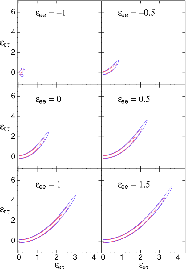
Figure 1: Sections of the function $\chi^{2}(\mathrel{{\epsilon_{ee}}},\mathrel{{\epsilon_{\tau\tau}}},\mathrel{{\epsilon_{e\tau}}})$ along the planes of fixed $\mathrel{{\epsilon_{ee}}}$ (numbers in the Figure), from a combined fit of the atmospheric and K2K data. The epsilons shown are per electron. The vacuum parameters $\theta_{23}$ and $\Delta m^{2}_{32}$ are marginalized over. The latter is taken to be negative (inverted mass hierarchy). We have also used $\theta_{13}=0$ and neglected effects of the smaller mass splitting, $\Delta m^{2}_{21}=0$. The contours, from the inner to the outer, correspond to $95\%,99\%$ and $3\sigma$ C.L. Only the positive $\mathrel{{\epsilon_{e\tau}}}$ semi-plane is shown in each case for visual convenience; the negative $\mathrel{{\epsilon_{e\tau}}}$ semi-plane is symmetric. More generally, the results are independent of the complex phase of $\mathrel{{\epsilon_{e\tau}}}$.

We performed a quantitative analysis of the atmospheric neutrino data with five parameters: two “vacuum” ones, $(\Delta m^{2}_{32},\theta_{23})$, and three NSI quantities $(\mathrel{{\epsilon_{ee}}},\mathrel{{\epsilon_{e\tau}}},\mathrel{{\epsilon_{\tau\tau}}})$, where $\mathrel{{\epsilon_{e\tau}}}$ has been treated as real for simplicity. The parameter space was scanned and a goodness-of-fit analysis was performed for each grid point.

In the analysis, we have used two types of codes. For many of the preliminary investigations we used our own code, which made several simplifying assumptions, but was designed to capture the relevant physical features of the atmospheric neutrinos in different energy ranges. For the final fits, we used a binary of the atmospheric neutrino program kindly provided to us by Michele Maltoni (SUNY, Stony Brook). This binary is essentially the same program used in our earlier paper Friedland:2004ah . It uses the complete 1489-day charged current Super-Kamiokande phase I data set Hayato (2004), including the $e$-like and $\mu$-like data samples of sub- and multi-GeV contained events (each grouped into 10 bins in zenith angle) as well as the stopping (5 angular bins) and through-going (10 angular bins) upgoing muon data events. This amounts to a total of 55 data points. For the calculation of the expected rates the code adopts the three-dimensional atmospheric neutrino fluxes given in Ref. Honda et al. (2004). The statistical analysis of the data follows the appendix of Ref. Gonzalez-Garcia and Maltoni (2004). The binary underwent extensive testing in the course of this project and the feedback was reported back to the author.

We have included the results of the K2K data analysis in our study, by adding our atmospheric $\chi^{2}$ to the K2K $\chi^{2}$ in the space of $\theta_{23}$ and $\Delta m^{2}_{32}$. The latter was provided by the K2K collaboration in tabular form, and refers to the published analysis of Ref. Aliu et al. (2004) (Fig. 4 there).

It is important to point out that in our analysis we use only NSI propagation effects. The detection effects are purposefully left out. The reason for this is that the changes in the detection cross sections due to NSI do not uniquely follow from the propagation effects, but depend on additional parameters and assumptions. As a result, the detection effects can vary significantly, from large to unobservable, depending on the underlying model of the NSI.

IV.1.1 NSI and detection effects

Let us give a detailed argument for why possible NSI effects on the detection cross sections are not directly related to the propagation effects. A reader primarily interested in the results of our numerical analysis may wish to skip to Sect IV.2.

Consider how the Super-Kamiokande collaboration extracts NC information from their data. One method is to analyze a multi-ring dataset specifically enriched with NC events through a careful sequence of cuts Fukuda et al. (2000); phd1 . Another method is to compare the rate of single $\pi^{0}$ events, most of which are produced in NC interactions, to the muon rate phd2 . In principle, only the collaboration can reliably model these data. Nevertheless, in what follows we set this consideration aside and ask: Can one in principle use these data to improve the bounds on NSI derived from propagation effects?

The multi-ring dataset. The main contribution to this dataset is from multi-pion production in the energy range $0.5-10$ GeV phd1 . While the exact expression for the cross-section is quite complicated (SK uses a semi-empirical formula), a qualitative estimate may be obtained by assuming deep inelastic neutrino-parton scattering. In this case, the cross-section depends on the squares of the left- and right-handed couplings, $g_{L}^{2}$ and $g_{R}^{2}$ Fukugita and Yanagida . It is immediately obvious that the result depends on how the NSI effects are distributed between the $u$ and $d$ quarks. The value of the axial coupling, $g_{A}=g_{L}-g_{R}$, is also crucial (the refraction effects fix only the vector part, $g_{V}=g_{L}+g_{R}$). For example, for the point used in Friedland:2004pp , splitting NSI evenly between $g_{L}$ and $g_{R}$ and assuming the standard value for $g_{A}$, we find an increase in the cross-section of only 20%. The effect becomes even smaller once the axial coupling is adjusted to compensate the increase given by the vector part. Hence, no rigorous constraint can be obtained from this sample.

The single $\pi^{0}$ sample. The main contribution to the single $\pi^{0}$ sample is from incoherent single pion production, followed by coherent single pion production phd2 . The first process is dominated by the $\Delta$ resonance and is largely controlled by the size of the axial coupling Fukugita and Yanagida . The second one is also axial: the neutral current creates a pion that scatters on the nucleus Rein and Shegal (1999). Hence, this sample would not constrain the vector interaction that is responsible for the modified matter effect. Also, it should be mentioned that the statistics in this sample is not sufficient to even separate the active-active from active-sterile scenarios. (The latter is disfavored by only $1.3\sigma$, see phd2 .)

Lastly, a simple observation is that if the NSI are assigned to electrons, they have no effect on the NC event rate in the detector, since the latter is dominated by scattering on nuclei. This makes especially clear that the propagation and detection effects need not be correlated. Only if strong model-dependent assumptions are made, like in the case of a sterile neutrino, can the two be used together to exclude an oscillation scenario.

We emphasize that it is important for Super-Kamiokande and other neutrino oscillation experiments to be looking for any anomalous NC signal: an observation of such signal would imply the discovery of NSI. At the same time, as the preceding examples show, a lack of such anomalous signal would not guarantee there are no NSI propagation effects.

IV.2 Main results: NSI, mixing and mass splitting

Our main result involves a scan of the $(\epsilon_{ee},\epsilon_{e\tau},\epsilon_{\tau\tau},\Delta m^{2}_{32},\theta_{23})$ space for real $\mathrel{{\epsilon_{e\tau}}}$, inverted mass hierarchy ($\Delta m^{2}_{32}<0$), $\theta_{13}=0$ and $\Delta m^{2}_{21}=0$. Variations of the three latter parameters represent subdominant effects; the cases of different mass hierarchy and nonzero $\theta_{13}$ are treated later, in Sect. IV.3.

The scan yields a five-dimensional allowed region. Various projections of this region are described next, in Figs. 1-5.

The first result is the region allowed by the data in the space of the NSI. It was found by marginalizing the $\chi^{2}$ function over the vacuum oscillation parameters. The resulting function, $\chi^{2}(\mathrel{{\epsilon_{ee}}},\mathrel{{\epsilon_{e\tau}}},\mathrel{{\epsilon_{\tau\tau}}})$, gives a 3-dimensional allowed region, two-dimensional $(\mathrel{{\epsilon_{e\tau}}},\mathrel{{\epsilon_{\tau\tau}}})$ sections of which are shown in Fig. 1 (the values of $\mathrel{{\epsilon_{ee}}}$ for each section are shown in the Figure). As the region is invariant under $\mathrel{{\epsilon_{e\tau}}}\leftrightarrow-\mathrel{{\epsilon_{e\tau}}}$, only the positive $\mathrel{{\epsilon_{e\tau}}}$ halves are shown for each section. The symmetry in the sign (phase) of $\mathrel{{\epsilon_{e\tau}}}$ is understood in terms of the oscillations probabilities, that were shown to depend on the absolute value of $\mathrel{{\epsilon_{e\tau}}}$ only (see sec. III.2).

The curves in the Figure are isocontours of $\Delta\chi^{2}\equiv\chi^{2}-\chi^{2}_{min}=7.81,11.35,14.16$ (from the inner to the outer), corresponding to $95\%,99\%$ and $3\sigma$ C.L. The parabolic flat direction in the function $\chi^{2}(\mathrel{{\epsilon_{ee}}},\mathrel{{\epsilon_{e\tau}}},\mathrel{{\epsilon_{\tau\tau}}})$ predicted by Eq. (17) is clearly seen. This direction is essentially determined by the atmospheric data, and is not altered significantly by the contribution of K2K (which, however, changes the extent of the region, as will be explained). The width of the parabolic region matches well the condition on the matter eigenvalues, Eq. (19), as was shown explicitly in Fig. 1 of ref. Friedland:2004ah . The points where the region (at a given C.L.) ends along the parabola well follow isocontours of the angle $\beta$ (specifically, $\cos^{2}\beta\simeq 0.30,0.35,0.42$ for the three confidence level contours in the figure), as expected from the “cutoff” conditions given by the low energy atmospheric sample and by the K2K results, Eqs. (22) and (23).

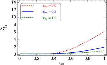
Figure 2: The difference $\Delta\chi^{2}$ (where $\chi^{2}$ is the same function of Fig. 1) plotted along the parabolic direction of Eq. (17), for three fixed values of $\mathrel{{\epsilon_{ee}}}$ (see legend).

Along the parabola, the function $\chi^{2}(\mathrel{{\epsilon_{ee}}},\mathrel{{\epsilon_{e\tau}}},\mathrel{{\epsilon_{\tau\tau}}})$ varies very slowly near the origin, and starts to increase appreciably only at $\epsilon_{e\tau}$ of about 0.5 or so. For example, we have: $\chi^{2}(0,0,0)=148.11$ (no NSI) and $\chi^{2}(0.73,0.35,0.07)=148.07$. The latter happens to be the absolute minimum, $\chi^{2}_{min}$, but clearly has practically the same goodness of fit as the origin. The curves Fig. 2 show how $\Delta\chi^{2}$ varies with $\mathrel{{\epsilon_{e\tau}}}$ along the parabola (17) for three fixed values of $\mathrel{{\epsilon_{ee}}}$.

As a side comment, we notice that the agreement with Eqs. (17) and (19) becomes worse with the decrease of $\mathrel{{\epsilon_{ee}}}$. This makes sense because as $\mathrel{{\epsilon_{ee}}}$ approaches $-1$, the two matter eigenvalues $\lambda_{e^{\prime}}$ and $\lambda_{\tau^{\prime}}$ have comparable size, thus breaking the approximation of hierarchy of the eigenvalues used in our derivations (sec. III.1). Notice that the panel with $\mathrel{{\epsilon_{ee}}}=-1$ shows a hint of transition from an upward to a downward parabolic region. This transition is expected to happen with the change of sign of the term $1+\mathrel{{\epsilon_{ee}}}$ in the matter Hamiltonian.

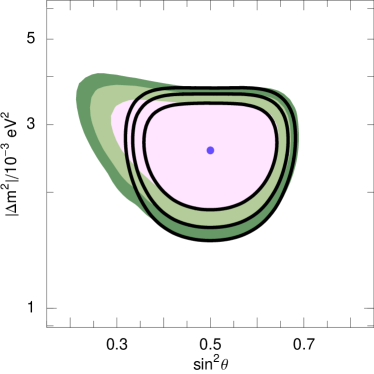
Figure 3: The shaded areas represent the regions in the space of $|\Delta m^{2}_{31}|$ and $\sin^{2}\theta_{23}$ allowed by the atmospheric neutrino and K2K data, obtained upon marginalizing over the NSI parameters. The regions correspond to the 95%, 99% and $3\sigma$ confidence levels for 2 d.o.f. (innermost to outermost). We have marginalized also over the sign of $\Delta m^{2}_{31}$ and took $-1.6\leq\mathrel{{\epsilon_{ee}}}\leq 1.6$, motivated by one of the accelerator bounds (see text). The corresponding regions obtained with purely standard interactions are shown for comparison.

The second result is the allowed region in the space of $\theta_{23}$ and $|\Delta m^{2}_{31}|$, obtained by marginalizing over the NSI parameters. This region is shown in Fig. 3. In the marginalization procedure we have restricted $\mathrel{{\epsilon_{ee}}}$ in the interval $-1.6\leq\mathrel{{\epsilon_{ee}}}\leq 1.6$. This serves as an example, and corresponds to the CHARM bound if the NSI are present exclusively as flavor-preserving interactions of $\mathrel{{\nu_{e}}}$ on the right-handed down quark Davidson et al. (2003) . We have marginalized also over the sign of $\Delta m^{2}_{31}$, thus including both mass hierarchies. Expectedly, with respect to the standard case, the allowed region is bigger, and extends to smaller mixing ($\sin^{2}\theta_{23}\simeq 0.2$ instead then $\sin^{2}\theta_{23}\simeq 0.31$) and slightly larger $|\Delta m^{2}_{31}|$, in agreement with the analytic considerations (sec. III). The absolute minimum lies at $|\Delta m^{2}_{31}|=2.6\times 10^{-3}$ eV², $\sin^{2}\theta=0.5$.

We find that the contours in the figure practically coincide with those obtained for normal hierarchy with $\mathrel{{\epsilon_{ee}}}$ fixed at the upper limit, $\mathrel{{\epsilon_{ee}}}=1.6$. Since this upper limit is determined by accelerator experiments, improvements of the accelerator NSI bounds would lead to a better knowledge of the oscillation parameters.

In the Table 1 we list the intervals allowed, at different confidence levels, for each vacuum parameter after marginalizing over all the other quantities. They exhibit features analogous to those of fig. 3. The results for the standard case are given, too, for comparison.

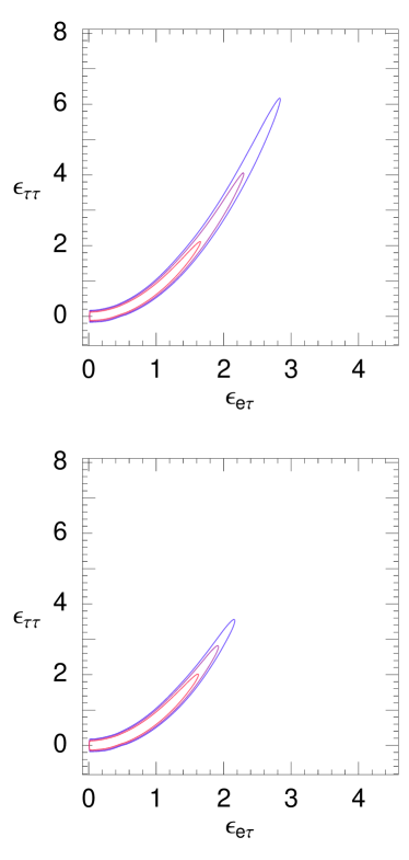
Figure 4: A section of the function $\chi^{2}(\mathrel{{\epsilon_{ee}}},\mathrel{{\epsilon_{\tau\tau}}},\mathrel{{\epsilon_{e\tau}}})$ along the plane $\mathrel{{\epsilon_{ee}}}=0.3$, from a fit to atmospheric data only (upper) and the combined fit of atmospheric and K2K data (lower). All the considerations made for Fig. 1 apply here.

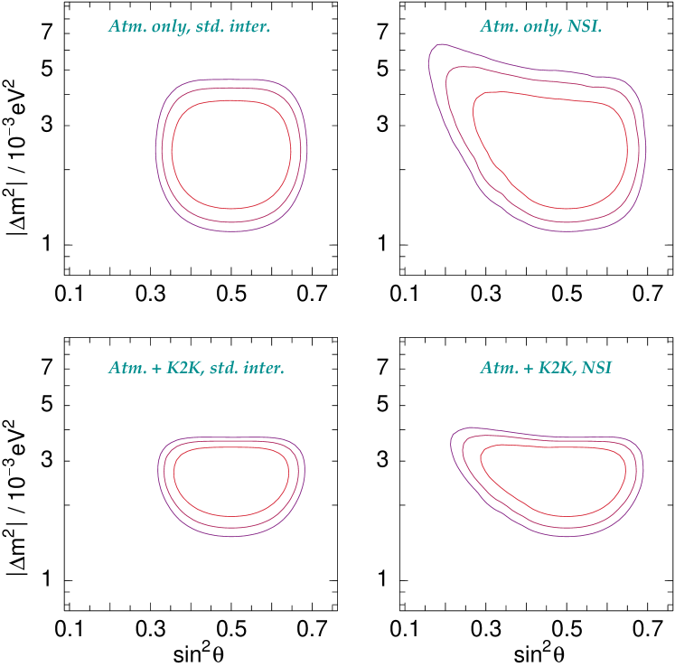
Figure 5: A more detailed version of Fig. 3, where the results of fitting the atmospheric data only and atmospheric+K2K are given for both the standard case and the case with NSI.

The K2K results play an important role in restricting both the region of the oscillations parameters and that of the NSI couplings. This is shown in Figs. 4 and 5. Figure 4 shows a representative section of $\chi^{2}(\mathrel{{\epsilon_{ee}}},\mathrel{{\epsilon_{\tau\tau}}},\mathrel{{\epsilon_{e\tau}}})$ (the same function as in Fig. 1) along the plane $\mathrel{{\epsilon_{ee}}}=0.3$. The lower panel refers to the full atmospheric+K2K fit (like all the results in Figs. 1-3), while the upper one is obtained with atmospheric data only. The reduction due to K2K is evident: for example, the edge of the $3\sigma$ contour changes from $(\mathrel{{\epsilon_{e\tau}}},\mathrel{{\epsilon_{\tau\tau}}})\simeq(2.8,6.0)$ to $(\mathrel{{\epsilon_{e\tau}}},\mathrel{{\epsilon_{\tau\tau}}})\simeq(2.2,3.8)$. The effect is smaller for smaller NSI, as one can see that the $95\%$ C.L. contour is practically unchanged between the two panels.

Fig. 5 is a series of variations of Fig. 3: the results of the fit in the plane $|\Delta m^{2}_{31}|$-$\sin^{2}\theta_{23}$ are shown with and without NSI, each with and without the inclusion of the K2K results. We see that with NSI the K2K data contribute to restrict the parameters, especially in the region of large $|\Delta m^{2}_{31}|$ and small mixing. The $3\sigma$ contour of this region is moved from $(\sin^{2}\theta_{23},|\Delta m^{2}_{31}|)\simeq(0.15,6\cdot 10^{-3}~{}{\rm eV^{2}})$ to $(\sin^{2}\theta_{23},|\Delta m^{2}_{31}|)\simeq(0.21,4\cdot 10^{-3}~{}{\rm eV^{2}})$. We also observe a restriction of $|\Delta m^{2}_{31}|$ from below, which is essentially the same in the cases with and without NSI.

IV.3 Subdominant effects: mass hierarchy, $\theta_{13}$, three neutrino corrections

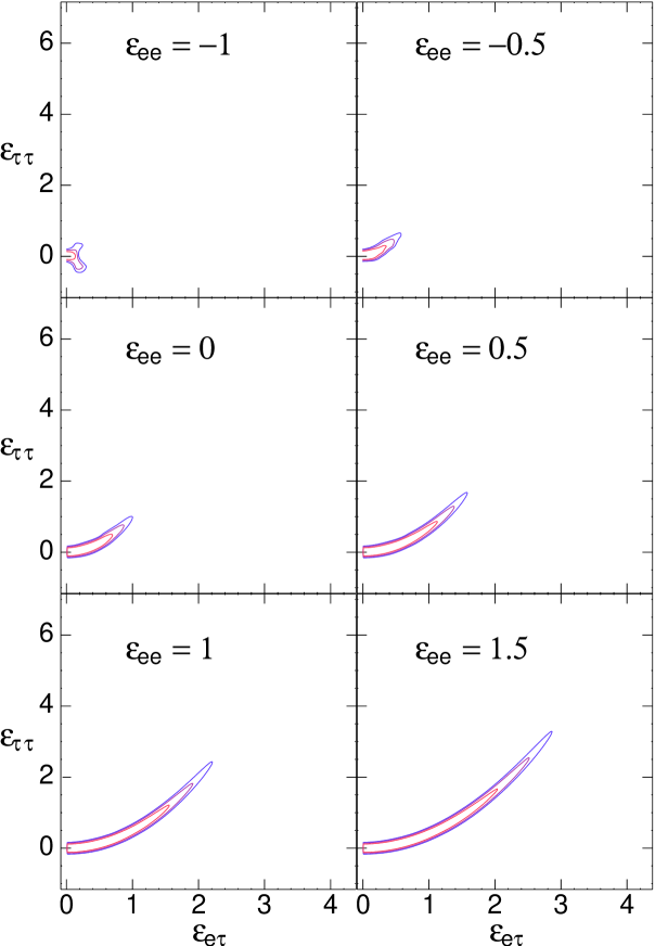
Figure 6: The same as Fig. 1 for normal mass hierarchy.

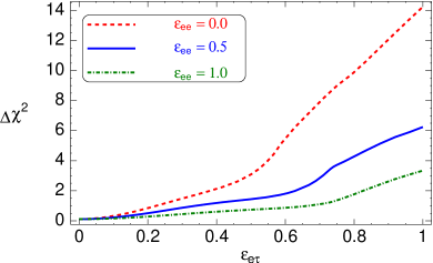
Figure 7: The same as Fig. 2 for normal mass hierarchy.

Here we generalize our results to include subdominant effects, namely the effect of the sign of the mass hierarchy, of a non-zero $\theta_{13}$ and of the 1-2, “solar”, oscillation parameters.

Fig. 6 shows the allowed region in the space of the NSI parameters for normal mass hierarchy. Analogously to the case of inverted hierarchy shown in Fig. 1, the region follows the parabola (17) and its endpoints follow isocontours of $\beta$. The main difference is that for normal hierarchy these isocontours are more restricted, i.e., the allowed range of NSI is smaller. Along the parabola, the $\chi^{2}$ grows faster with the epsilons for normal hierarchy, as shown in Fig. 7. For example, if $\mathrel{{\epsilon_{ee}}}=0$, the $3\sigma$ C.L. contour ends at $(\mathrel{{\epsilon_{e\tau}}},\mathrel{{\epsilon_{\tau\tau}}})\sim(1.0,1.0)$ for normal hierarchy, while we have $(\mathrel{{\epsilon_{e\tau}}},\mathrel{{\epsilon_{\tau\tau}}})\sim(1.8,2.5)$ for inverted hierarchy. In terms of $\cos^{2}\beta$, the contours in Fig. 6 correspond to $\cos^{2}\beta\simeq 0.47,0.53,0.65$ (compared with $\cos^{2}\beta\simeq 0.30,0.35,0.42$ for Fig. 1).

From our analytics, we can see two sources of difference between the results for the two hierarchies. One traces back to the term $\lambda_{\tau^{\prime}}/\Delta$ in the 3-3 entry of the Hamiltonian (14) (see also Eq. (15)). This can be as large as $\lambda_{\tau^{\prime}}/\Delta\sim 0.2$ in the allowed region of parameters (Eq. (19)) and so is expected to contribute at the subdominant level. Secondly, corrections that depend on the sign of $\Delta$ arise also from the small, but not zero, coupling of the state $\mathrel{{\nu_{e}}}^{\prime}$ with the other two. This depends on the 1-1 entry of the Hamiltonian (14) and therefore on the relative sign of $\lambda_{e^{\prime}}$ and $\Delta$. Considering that the data are dominated by neutrinos over antineutrinos (due to the larger detection cross section, see e.g. Fukugita and Yanagida ), it makes sense that a larger allowed region of NSI is obtained for inverted hierarchy, where, for neutrinos, matter and vacuum terms have the same sign and thus suppress the mixing of $\mathrel{{\nu_{e}}}^{\prime}$ more than in the normal hierarchy case.

Fig. 8 shows a generalization of Fig. 1 to non-zero $\theta_{13}$. Only the plane $\mathrel{{\epsilon_{ee}}}=0$ is shown for illustration. The plot was obtained for $\theta_{13}$ at the reactor limit, Eq. (6), with $\theta_{13}>0$. From the comparison of Figs. 8 and 1 it is clear that $\theta_{13}$ breaks the symmetry in the sign of $\mathrel{{\epsilon_{e\tau}}}$. While the parabolic direction of the region is unchanged, the position where the region ends along this direction is affected. These features can be understood analytically, as shown in Appendix A. The effect of non-zero $\theta_{13}$ on the extent of the allowed region in the space of $|\Delta m^{2}_{31}|$-$\sin^{2}\theta_{23}$ is small and is not shown here.

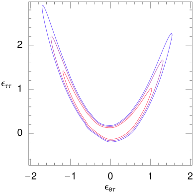
Figure 8: An example of how the contours of Fig. 1 change with non-zero $\theta_{13}$. This plot refers to $\mathrel{{\epsilon_{ee}}}=0$ and $\sin^{2}\theta_{13}=0.02$, with $\theta_{13}>0$.

Let us now comment on conversion effects in the lowest energy part of the atmospheric neutrino spectrum, corresponding to the sub-GeV events. Here oscillations driven by the $\Delta m^{2}_{21}$ vacuum terms and matter terms occur on top of faster vacuum oscillations due to $\Delta m^{2}_{32}$. The result is a deviation of the sub-GeV e-like events from the unoscillated prediction. This effect has been discussed in detail for the standard, no-NSI case Peres and Smirnov (1999, 2004); Gonzalez-Garcia et al. (2004). It was found that the ratio of the fluxes of neutrinos of muon and electron flavors depends on $\Delta m^{2}_{21}$ through the probability $P(\nu_{2}\rightarrow\mathrel{{\nu_{e}}})$ of conversion of the mass eigenstate $\nu_{2}$ into $\mathrel{{\nu_{e}}}$ inside the Earth. This probability is multiplied by the flux factor ${\cal F}=r\cos^{2}\theta_{23}-1$, with $r$ being the unoscillated ratio on muon and electron neutrino fluxes. The numerical coincidence $\cos^{2}\theta_{23}\sim 1/2$ and $r\sim 2$ produces a strong suppression of ${\cal F}$ and thus of the conversion effect Peres and Smirnov (1999).

The generalization of this to NSI is immediate. Given the smallness of the effect on absolute scale, with an impact on the fit to the data not larger than few per cents, we choose not to discuss it in detail. We mention two sources of enhancement of the conversion effect. The first is a possibly larger flux factor, due to a smaller $\theta_{23}$, see sec. IV.2. The second is a larger probability $P(\nu_{2}\rightarrow\mathrel{{\nu_{e}}})$ due to NSI. Indeed, if flavor-changing NSI are present, $P(\nu_{2}\rightarrow\mathrel{{\nu_{e}}})$ converges to a non-zero value when matter terms dominate over the vacuum ones, in contrast with the standard scenario (see e.g. Friedland:2004pp ).

Finally, it should be pointed out that there exists an important identification in the parameter space. Indeed, physical results depend only on the relative sign of the vacuum and matter terms of the Hamiltonian. Because of this, for vanishing $\theta_{13}$, the case of one hierachy maps onto the case of the other hierarchy with $\mathrel{{\epsilon_{ee}}}\leftrightarrow-2-\mathrel{{\epsilon_{ee}}}$, $\mathrel{{\epsilon_{e\tau}}}\rightarrow-\mathrel{{\epsilon_{e\tau}}}$, $\mathrel{{\epsilon_{\tau\tau}}}\leftrightarrow-\mathrel{{\epsilon_{\tau\tau}}}$. This, even though we have presented only the cases $\mathrel{{\epsilon_{ee}}}\geq-1$, our results extend to $\mathrel{{\epsilon_{ee}}}<-1$. Explicitly, normal hierachy with $\mathrel{{\epsilon_{ee}}}<-1$ maps to inverted hierarchy with $\mathrel{{\epsilon_{ee}}}>-1$, and, likewise, inverted hierachy with $\mathrel{{\epsilon_{ee}}}<-1$ maps to normal hierarchy with $\mathrel{{\epsilon_{ee}}}>-1$. The cases $\mathrel{{\epsilon_{ee}}}=-1$ for the two hierarchies, shown in Figs. 1 and 6, are clearly related by the transformation $\mathrel{{\epsilon_{\tau\tau}}}\leftrightarrow-\mathrel{{\epsilon_{\tau\tau}}}$ (and also $\mathrel{{\epsilon_{e\tau}}}\leftrightarrow-\mathrel{{\epsilon_{e\tau}}}$, but the region is symmetric with respect to this tranformation).

V Summary and conclusions

We have explored the sensitivity of the atmospheric and K2K neutrino data to neutrino NSI in the $e-\tau$ sector, and investigated how the presence of NSI can change the allowed region of the vacuum oscillation parameters. The results can be summarized as follows:

1. The region of the NSI parameters $\mathrel{{\epsilon_{ee}}},\mathrel{{\epsilon_{\tau\tau}}},\mathrel{{\epsilon_{e\tau}}}$ allowed by the data is essentially determined by two conditions on the neutrino-matter interaction Hamiltonian. The first condition is that one of the eigenvalues not exceed the vacuum term at high energy ($E\sim 20-30$ GeV): $|\lambda_{\tau^{\prime}}|/\Delta\mathrel{\vbox{\hbox{$<$}\nointerlineskip\hbox{$\sim$}}}1$ or, numerically, $|\lambda_{\tau^{\prime}}|\mathrel{\vbox{\hbox{$<$}\nointerlineskip\hbox{$\sim$}}}5\cdot 10^{-14}$ eV. It explains the presence of a “flat direction” in the $\chi^{2}$, which extends the allowed region to large NSI couplings. This direction is a parabola on planes of constant $\mathrel{{\epsilon_{ee}}}$. Transversely to it, the $\chi^{2}$ function grows rapidly, as can be seen from our figures. The second condition is on the mixing angle that describes the flavor composition of the eigenstates of the matter Hamiltonian: $\beta\mathrel{\vbox{\hbox{$<$}\nointerlineskip\hbox{$\sim$}}}0.3\pi\simeq 57^{\circ}$. It follows from requiring consistency between atmospheric data samples of different energy and/or between the atmospheric data and the (practically) matter-free K2K results. This condition explains the worsening of the fit along the parabolic flat direction.

   In terms of the epsilons, we see that the allowed range of $\mathrel{{\epsilon_{e\tau}}}$ and $\mathrel{{\epsilon_{\tau\tau}}}$ strongly depends on the value of $\mathrel{{\epsilon_{ee}}}$, which in turn is unconstrained by atmospheric neutrinos. Both $\mathrel{{\epsilon_{e\tau}}}$ and $\mathrel{{\epsilon_{\tau\tau}}}$ are most constrained for $\mathrel{{\epsilon_{ee}}}=-1$, and the constraint rapidly weakens as $\mathrel{{\epsilon_{ee}}}$ is increased. For $\mathrel{{\epsilon_{ee}}}=1.5$ and inverted mass hierarchy, values as large as $\mathrel{{\epsilon_{\tau\tau}}}\sim 5$ and $|\mathrel{{\epsilon_{e\tau}}}|\sim 3.5$ are allowed along the parabola. These would translate into very loose limits on the NSI parameters of the effective four-fermion Lagrangian. Still, such limits generally improve on existing accelerator bounds.

2. The inclusion of NSI in the analysis modifies the allowed region of the vacuum oscillation parameters, $\sin^{2}\theta_{23}$ and $\Delta m^{2}_{31}$. As our analytical treatment shows, the fit to large NSI is achieved at the expense of changing the values of the vacuum oscillation parameters. After marginalizing over the NSI couplings and the sign of the mass squared splitting, we find that the region in the space of $\sin^{2}\theta_{23}$ and $|\Delta m^{2}_{31}|$ is larger than that of the standard, no-NSI case. Smaller mixing and larger mass splitting are allowed. If we fit the data to one parameter at a time, and marginalize over all the others (see Table 1) we find the intervals $\sin^{2}\theta_{23}=0.24-0.68$ and $|\Delta m^{2}_{31}|=(1.7-3.9)\cdot 10^{-3}~{}{\rm eV^{2}}$ at $3\sigma$ C.L. ( to be compared to the results of the standard case: $\sin^{2}\theta_{23}=0.32-0.66$ and $|\Delta m^{2}_{31}|=(1.7-3.6)\cdot 10^{-3}~{}{\rm eV^{2}}$).

3. The recent K2K results play an important role in limiting NSI. This stems from the fact that for the K2K setup matter effects are negligible, and therefore K2K measures the true vacuum oscillations parameters. The K2K constraint on the oscillation parameters, particularly on $|\Delta m^{2}_{31}|$, translates in a constraint on NSI, by limiting the range over which the oscillation parameters could be varied to compensate for the effects of large NSI. As an example, for $\mathrel{{\epsilon_{ee}}}\sim{\cal O}(10^{-1})$, the addition of the K2K results restricts the region of the NSI couplings by about $\sim 25\%$ in the direction of $\mathrel{{\epsilon_{\tau\tau}}}$ (Fig. 4), with respect to the analysis of atmospheric neutrinos only.

4. We have studied the dependence of the results on the mass hierarchy (sign of $\Delta m^{2}_{31}$). The allowed region of the NSI couplings has the same shape for both hierarchies, but, for $\mathrel{{\epsilon_{ee}}}\mathrel{\vbox{\hbox{$>$}\nointerlineskip\hbox{$\sim$}}}-1$, it is more extended for the inverted hierarchy by up to a factor of $\sim 2$ in the direction of $\mathrel{{\epsilon_{\tau\tau}}}$. Subdominant effects due to $\theta_{13}$ have been analyzed. They mainly break the degeneracy in the sign (phase) of $\mathrel{{\epsilon_{e\tau}}}$. Corrections due to the smaller mass squared splitting, $\Delta m^{2}_{21}$, turn out to be quite small.

Our results represent a step toward the reconstruction of the region in the space of NSI couplings that is compatible with all existing data. One of the next steps is the extension of the analysis to include the solar neutrino and KamLAND data. While it is known that the latter do not exclude large NSI couplings along the parabolic region (17) Friedland:2004pp , a detailed study has not been done before; it is presented in a companion paper of this work, soon to be completed Friedland and Lunardini .

The fact that still large NSI in the $e-\tau$ sector are not experimentally excluded has important implications for other aspects of neutrino physics. First, it is an important motivation for neutrino experiments with man-made sources. Experiments with neutrino beams of short or intermediate base-line, such as MINOS Thomson (2005) or OPERA Autiero (2005) will have negligible matter effects, and will increase the precision of the measurement of $\theta_{23}$ and $|\Delta m^{2}_{31}|$. This increased precision will leave even less room for NSI, or give indication of their existence, depending on whether the measured vacuum parameters are in agreement or in tension (especially if the tension is in the direction of smaller mixing and/or larger mass splitting) with the analysis of atmospheric neutrino with standard interactions only.

Neutrino beams with energy $E\sim 1-10$ GeV and long base-line (of the order of thousands of Km) like the proposed Fermilab-to-Soudan design, for example, would exhibit dramatic effects of NSI in the disappearance of muon neutrinos (or antineutrinos) as well as in the appearance channel $\mathrel{{\nu_{\mu}}}\rightarrow\mathrel{{\nu_{e}}}$ (or $\mathrel{{\bar{\nu}}_{\mu}}\rightarrow\mathrel{{\bar{\nu}}_{e}}$). In the disappearance channel NSI would produce an irregular pattern of oscillations minima and maxima, due to all three neutrinos being involved in the oscillations, in contrast with the simpler two-neutrino $\mathrel{{\nu_{\mu}}}\rightarrow\mathrel{{\nu_{\tau}}}$ oscillations expected in absence of NSI. The appearance channel $\mathrel{{\nu_{\mu}}}\rightarrow\mathrel{{\nu_{e}}}$ would be particularly characteristic in the fact that the $\mathrel{{\nu_{e}}}$ component could be much larger than what allowed by standard interactions and subdominant effects (those of $\theta_{13}$ and of $\Delta m^{2}_{21}$) and would not be suppressed at high energy – in contrast with the case of the MSW effect with standard interactions – as a consequence of flavor-changing NSI. In the high-energy limit, i.e. where the matter potential in the Earth dominates over vacuum terms, the amplitude of the $\mathrel{{\nu_{\mu}}}\rightarrow\mathrel{{\nu_{e}}}$ oscillation would be controlled by the matter mixing $\beta$:

$$P(\mathrel{{\nu_{\mu}}}\rightarrow\mathrel{{\nu_{e}}})\sim\sin^{2}\beta P(\mathrel{{\nu_{\mu}}}\rightarrow\nu_{\tau}^{\prime})~{},$$ (25)

where $P(\mathrel{{\nu_{\mu}}}\rightarrow\mathrel{{\nu_{\tau}}}^{\prime})$ is given in Eq. (16) and is unsuppressed at high energy for NSI along the parabola (17).

The presence of NSI can also alter significantly the physics of supernova neutrinos, in a way that may be tested with data from a future galactic supernova. Firstly, in the outer regions of the collapsing star, the NSI couplings may produce a richer structure of level-crossings with respect to the two MSW resonances of the standard case. New resonances may, in principle, appear depending on the chemical composition of the medium in the star and on what scatterers are responsible for the NSI. A less trivial effect will be on the evolution of trapped neutrinos inside the core of the protoneutron star. Here, NSI may affect the explosion itself, by changing the dynamics of the core and the energetics of the shock wave. This fundamental effect has been overlooked until recently Amanik et al. (2004). More work is required to understand the full implications of NSI, including possible changes in the r-processes and in the energy deposition by neutrinos in the matter of the star.

Appendix A Estimating corrections due to $\theta_{13}$

As seen in Fig. 8, the effect of nonzero $\theta_{13}$ is to break the $\mathrel{{\epsilon_{e\tau}}}\leftrightarrow-\mathrel{{\epsilon_{e\tau}}}$ symmetry, while preserving the general parabolic shape of the region. These features can be understood by generalizing our analytical description of Sec. III.2. The corrections due to $\theta_{13}$ enter the vacuum part of the Hamiltonian, and therefore influence those predictions that depend on vacuum terms, like the mixing and mass splitting in matter, Eq. (15), and the “cutoff” conditions (22) and (23). One expects an interplay between $\mathrel{{\epsilon_{e\tau}}}$ terms and $\theta_{13}$ terms, since both couple $\mathrel{{\nu_{e}}}$ to $\mathrel{{\nu_{\tau}}}$. This interplay has the form of an additive interference, analogous to the one involving the vacuum terms and the standard interaction in the MSW effect. This is the origin of the breaking of the symmetry in the sign (phase) of $\mathrel{{\epsilon_{e\tau}}}$.

Expanding the Hamiltonian in Eq. (14) along the parabolic direction (17) to first order in $\sin 2\theta_{13}$, we find the generalizations of Eqs. (20) and (21):

$$\cos\theta\simeq\frac{1}{\sqrt{1+c^{2}_{\beta}}}+\frac{\sin 2\theta_{13}s_{2\beta}\cos(2\psi-\delta)}{4(1+c^{2}_{\beta})},$$

$$\Delta m^{2}\simeq\Delta m^{2}_{m}\frac{1+\cos^{-2}\beta}{2}\left[1+\frac{\sin 2\theta_{13}\tan\beta}{(1+\cos^{2}\beta)^{3/2}}\right].\;\;\;\;\;\;\;\;$$ (26)

As in Eqs. (20) and (21), these expressions give the values of the vacuum parameters that correspond to $\theta_{m}\simeq\pi/4$ and a given value of the mass splitting in matter, $\Delta m^{2}_{m}$.

The generalized form of the condition (22) is

$$-\sqrt{\frac{1}{\tan^{2}\theta}-1}-\sin 2\theta_{13}c_{\theta}\cos(2\psi-\delta)\mathrel{\vbox{\hbox{$<$}\nointerlineskip\hbox{$\sim$}}}\tan\beta\mathrel{\vbox{\hbox{$<$}\nointerlineskip\hbox{$\sim$}}}+\sqrt{\frac{1}{\tan^{2}\theta}-1}-\sin 2\theta_{13}c_{\theta}\cos(2\psi-\delta)~{}.$$ (27)

Eqs. (26)-(27) are accurate to the order $\sin 2\theta_{13}$, while ${\cal O}(\sin^{2}\theta_{13})$ or higher terms are not under control. We have neglected terms proportional to $\lambda_{\tau^{\prime}}/\Delta\ll 1$ (which is accurate along the parabola). The $\theta_{13}$ correction to Eq. (23) is more complicated and will not be given here. We notice that the $\theta_{13}$ term in Eqs. (26) comes as a product with $\sin\beta$ from an expansion of terms of the type $|A\sin\beta/\Delta+\sin\theta_{13}e^{i\delta}|^{2}$; this confirms the MSW-like interference mentioned above. One can also see how results depend on the relative phase $2\psi-\delta$ of the matter and vacuum terms. For $\theta_{23}$ in the first octant, $\psi=\delta=0$, and $\theta_{13}>0$ Eq. (27) gives a stronger restriction for positive rather than negative $\mathrel{{\epsilon_{e\tau}}}$. Similarly, from (26) we see that a positive $\mathrel{{\epsilon_{e\tau}}}$ would increase the ratio $\Delta m^{2}/\Delta m^{2}_{m}$, thus making the tension with the low-energy sample and/or with K2K stronger. Both of these features correspond to the trend observed in Fig. 8. We have checked that there is also quantitative agreement between numerical and analytical results (Eqs. (26)-(27)) at the order of magnitude level.

References

- (1) J. S. M. Ginges and V. V. Flambaum, Phys. Rept. 397, 63 (2004) [arXiv:physics/0309054].
- Brooks et al. (1999) M. L. Brooks et al. (MEGA), Phys. Rev. Lett. 83, 1521 (1999), eprint hep-ex/9905013.
- (3) G. W. Bennett et al. [Muon g-2 Collaboration], Phys. Rev. Lett. 89, 101804 (2002) [Erratum-ibid. 89, 129903 (2002)] [arXiv:hep-ex/0208001].
- (4) Y. Hayato et al. [Super-Kamiokande Collaboration], Phys. Rev. Lett. 83, 1529 (1999) [arXiv:hep-ex/9904020].
- Berezhiani and Rossi (2002) Z. Berezhiani and A. Rossi, Phys. Lett. B535, 207 (2002), eprint hep-ph/0111137.
- Vilain et al. (1994) P. Vilain et al. (CHARM-II), Phys. Lett. B335, 246 (1994).
- Zeller et al. (2002) G. P. Zeller et al. (NuTeV), Phys. Rev. Lett. 88, 091802 (2002), eprint hep-ex/0110059.
- Davidson et al. (2003) S. Davidson, C. Pena-Garay, N. Rius, and A. Santamaria, JHEP 03, 011 (2003), eprint hep-ph/0302093.
- Wolfenstein (1978) L. Wolfenstein, Phys. Rev. D17, 2369 (1978).
- Mikheev and Smirnov (1986) S. P. Mikheev and A. Y. Smirnov, Nuovo Cim. C9, 17 (1986).
- Mikheev and Smirnov (1985) S. P. Mikheev and A. Y. Smirnov, Sov. J. Nucl. Phys. 42, 913 (1985).
- Valle (1987) J. W. F. Valle, Phys. Lett. B199, 432 (1987).
- Guzzo et al. (1991) M. M. Guzzo, A. Masiero, and S. T. Petcov, Phys. Lett. B260, 154 (1991).
- Fornengo et al. (2002) N. Fornengo, M. Maltoni, R. T. Bayo, and J. W. F. Valle, Phys. Rev. D65, 013010 (2002), eprint hep-ph/0108043.
- Guzzo et al. (2002) M. Guzzo et al., Nucl. Phys. B629, 479 (2002), eprint hep-ph/0112310.
- (16) A. Friedland, C. Lunardini and C. Pena-Garay, Phys. Lett. B 594, 347 (2004) [arXiv:hep-ph/0402266].
- Guzzo et al. (2004) M. M. Guzzo, P. C. de Holanda, and O. L. G. Peres, Phys. Lett. B591, 1 (2004), eprint hep-ph/0403134.
- Gonzalez-Garcia and Maltoni (2004) M. C. Gonzalez-Garcia and M. Maltoni, Phys. Rev. D70, 033010 (2004), eprint hep-ph/0404085.
- Miranda et al. (2004) O. G. Miranda, M. A. Tortola, and J. W. F. Valle (2004), eprint hep-ph/0406280.
- de Gouvea and Pena-Garay (2004) A. de Gouvea and C. Pena-Garay (2004), eprint hep-ph/0406301.
- (21) A. Friedland, C. Lunardini and M. Maltoni, Phys. Rev. D 70, 111301 (2004) [arXiv:hep-ph/0408264].
- Fukuda et al. (1998) Y. Fukuda et al. (Super-Kamiokande), Phys. Rev. Lett. 81, 1562 (1998), eprint hep-ex/9807003.
- Fukuda et al. (2000) S. Fukuda et al. (Super-Kamiokande), Phys. Rev. Lett. 85, 3999 (2000), eprint hep-ex/0009001.
- Ashie et al. (2004) Y. Ashie et al. (Super-Kamiokande), Phys. Rev. Lett. 93, 101801 (2004), eprint hep-ex/0404034.
- Aliu et al. (2004) E. Aliu et al. (K2K) (2004), eprint hep-ex/0411038.
- Krastev and Petcov (1988) P. I. Krastev and S. T. Petcov, Phys. Lett. B205, 84 (1988).
- (27) T. K. Gaisser, “Cosmic Rays And Particle Physics,”, Cambridge, UK: Univ. Pr. (1990) 279 p.
- Gonzalez-Garcia and Nir (2003) M. C. Gonzalez-Garcia and Y. Nir, Rev. Mod. Phys. 75, 345 (2003), eprint hep-ph/0202058.
- (29) M. Fukugita and T. Yanagida , “Physics of neutrinos and applications to astrophysics”, Berlin, Germany: Springer (2003) 593 p.
- Kajita (2004) T. Kajita, New J. Phys. 6, 194 (2004).
- Gaisser et al. (1996) T. K. Gaisser et al., Phys. Rev. D54, 5578 (1996), eprint hep-ph/9608253.
- Bugaev et al. (1998) E. V. Bugaev et al., Phys. Rev. D58, 054001 (1998), eprint hep-ph/9803488.
- Fiorentini et al. (2001) G. Fiorentini, V. A. Naumov, and F. L. Villante, Phys. Lett. B510, 173 (2001), eprint hep-ph/0103322.
- Battistoni et al. (2003) G. Battistoni, A. Ferrari, T. Montaruli, and P. R. Sala, Astropart. Phys. 19, 269 (2003), eprint hep-ph/0207035.
- Barr et al. (2004) G. D. Barr, T. K. Gaisser, P. Lipari, S. Robbins, and T. Stanev, Phys. Rev. D70, 023006 (2004), eprint astro-ph/0403630.
- Honda et al. (2004) M. Honda, T. Kajita, K. Kasahara, and S. Midorikawa, Phys. Rev. D70, 043008 (2004), eprint astro-ph/0404457.
- Ambrosio et al. (1998) M. Ambrosio et al. (MACRO), Phys. Lett. B434, 451 (1998), eprint hep-ex/9807005.
- Ambrosio et al. (2000) M. Ambrosio et al. (MACRO), Phys. Lett. B478, 5 (2000), eprint hep-ex/0001044.
- Ambrosio et al. (2001) M. Ambrosio et al. (MACRO), Phys. Lett. B517, 59 (2001), eprint hep-ex/0106049.
- Allison et al. (1997) W. W. M. Allison et al., Phys. Lett. B391, 491 (1997), eprint hep-ex/9611007.
- Sanchez et al. (2003) M. C. Sanchez et al. (Soudan 2), Phys. Rev. D68, 113004 (2003), eprint hep-ex/0307069.
- Ashie et al. (2005) Y. Ashie et al. (Super-Kamiokande) (2005), eprint hep-ex/0501064.
- (43) C. Saji (Super-Kamiokande) , ICRC 2003 Proceedings. Edited by T. Kajita, Y. Asaoka, A. Kawachi, Y. Matsubara, M. Sasaki. Tokyo, Japan, Universal Academy Press, 2003. 8v. (Frontiers Science Series, No. 41, 43).
- Lipari and Lusignoli (1999) P. Lipari and M. Lusignoli, Phys. Rev. D60, 013003 (1999), eprint hep-ph/9901350.
- Fogli et al. (1999) G. L. Fogli, E. Lisi, A. Marrone, and G. Scioscia, Phys. Rev. D60, 053006 (1999), eprint hep-ph/9904248.
- Ahn et al. (2003) M. H. Ahn et al. (K2K), Phys. Rev. Lett. 90, 041801 (2003), eprint hep-ex/0212007.
- Eguchi et al. (2003) K. Eguchi et al. (KamLAND), Phys. Rev. Lett. 90, 021802 (2003), eprint hep-ex/0212021.
- (48) T. Araki et al. [KamLAND Collaboration], Phys. Rev. Lett. 94, 081801 (2005) [arXiv:hep-ex/0406035].
- (49) B. Aharmim et al. [SNO Collaboration], arXiv:nucl-ex/0502021.
- Apollonio et al. (1999) M. Apollonio et al. (CHOOZ), Phys. Lett. B466, 415 (1999), eprint hep-ex/9907037.
- Apollonio et al. (2003) M. Apollonio et al., Eur. Phys. J. C27, 331 (2003), eprint hep-ex/0301017.
- Boehm et al. (2001) F. Boehm et al., Phys. Rev. D64, 112001 (2001), eprint hep-ex/0107009.
- (53) A. Friedland and C. Lunardini, Phys. Rev. D 68, 013007 (2003) [arXiv:hep-ph/0304055].
- Mikheyev and Smirnov (1989) S. P. Mikheyev and A. Y. Smirnov, Prog. Part. Nucl. Phys. 23, 41 (1989).
- Kuo and Pantaleone (1989) T. K. Kuo and J. T. Pantaleone, Rev. Mod. Phys. 61, 937 (1989).
- Gonzalez-Garcia et al. (2004) M. C. Gonzalez-Garcia, M. Maltoni, and A. Y. Smirnov, Phys. Rev. D70, 093005 (2004), eprint hep-ph/0408170.
- Hayato (2004) Y. Hayato, Eur. Phys. J. C33, s829 (2004).
- (58) K. Ishihara [Super-Kamiokande Collaboration], Ph.D. thesis, University of Tokyo, Dec. 1999, available at http://www-sk.icrr.u-tokyo.ac.jp/doc/sk/pub/.
- (59) S. Nakayama, [Super-Kamiokande Collaboration], Ph.D. thesis, University of Tokyo, Feb 2003, available at http://www-sk.icrr.u-tokyo.ac.jp/doc/sk/pub/.
- Rein and Shegal (1999) D. Rein and L. M. Sehgal, Nucl. Phys. B223, 29 (1983).
- Peres and Smirnov (1999) O. L. G. Peres and A. Y. Smirnov, Phys. Lett. B456, 204 (1999), eprint hep-ph/9902312.
- Peres and Smirnov (2004) O. L. G. Peres and A. Y. Smirnov, Nucl. Phys. B680, 479 (2004), eprint hep-ph/0309312.
- (63) A. Friedland and C. Lunardini, in preparation.
- Thomson (2005) M. A. Thomson, Nucl. Phys. Proc. Suppl. 143, 249 (2005).
- Autiero (2005) D. Autiero (OPERA), Nucl. Phys. Proc. Suppl. 143, 257 (2005).
- Amanik et al. (2004) P. S. Amanik, G. M. Fuller, and B. Grinstein (2004), eprint hep-ph/0407130.
- Athanassopoulos et al. (1995) C. Athanassopoulos et al. (LSND), Phys. Rev. Lett. 75, 2650 (1995), eprint nucl-ex/9504002.
- Athanassopoulos et al. (1996) C. Athanassopoulos et al. (LSND), Phys. Rev. Lett. 77, 3082 (1996), eprint nucl-ex/9605003.
- Ray (2004) H. L. Ray (MiniBooNE) (2004), eprint hep-ex/0411022.