hep-th/0506144

Standard and Non-Standard Extra Matter for Non-Supersymmetric Unification
Alex Kehagias and N.D. Tracas
Physics Department, National Technical University,
Athens 157 73 , Greece

1 Introduction

Understanding the electroweak symmetry breaking is one of the most important problems in high energy physics. Ultimate connected with this is the new physics expected to be found in the forthcoming experiments. Many ideas have been proposed such as supersymmetry, extra dimensions e.t.c. Among these, weak scale supersymmetry is the most popular one, as among others, it gives answers for the gauge hierarchy problem, the origin of the electroweak symmetry breaking as well as it provides dark matter candidates. Moreover, it has a concrete prediction, namely, gauge coupling unification around $M_{U}\sim 10^{16}{\rm GeV}$. This fact has been considered as supporting evidence for both gauge unification and supersymmetry, pointing towards the idea that supersymmetry is indeed realized in nature.

However, one may want to extrapolate SM beyond the TeV threshold, demanding the celebrated features of supersymmetry, like gauge coupling unification and dark matter candidates, but without supersymmetry itself. In this case, we are facing the naturalness problem of the scalar sector, which makes this extrapolation above the TeV scale questionable. This is much like the cosmological constant and the naturalness problem connected with it, which however is ignored in all practical calculations. Similarly for the case at hand, one may assume that there is a mechanism which makes the TeV scale harmless and SM can be followed up to GUT energy scales. This line of though has recently be proposed in [1]. In this scenario, there is no low-scale supersymmetry but rather supersymmetry is realized at some intermediate scale $M_{S}$ and expected gauge unification still at the GUT scale $M_{U}$. This is an alternative to the MSSM with low-energy supersymmetry and it is known as split supersymmetry [1],[2],[3]. In the latter, all superpartners are pushed to the $M_{S}$, while only gauginos and Higgsinos remain at the weak scale. Apart from the latter, the fine-tuned Higgs as well as the fermions, which are protected by chiral symmetry, remains also near the electroweak scale. Clearly, this proposal violates the naturalness requirement for the Higgs mass and it seems to contradict the reason of introducing supersymmetry in first place. One may still assume that there exist still an unknown mechanism which permit the Higgs mass to remain around the weak scale. We recall at this point the cosmological constant problem mentioned above, where consistent calculations can be done ignoring the cosmological constant and any mechanism connected with it. Recently, split supersymmetry was shown to be realized also in string theory [4],[5].

We recall that supersymmetry is a basic ingredient of string theory and if supersymmetry is not realized at the TeV scale, it is more natural to be tight to the string scale. In particular, it is very difficult to justify the requirement of a supersymmetric spectrum as there is no reason for supersymmetry in first place if we assume that supersymmetry plays no role in the hierarchy problem. However, gauge coupling unification in the supersymmetric SM is an impressive aspect of supersymmetry and one may wondered if it is possible to achieved it in non-supersymmetric theories. The purpose of the present work is exactly to check if gauge coupling unification may be achieved by introducing extra matter (scalars and fermions) above the electroweak scale. We first analyse the general case finding out several irreps of extra matter which achieve gauge coupling unification. We then, by considering a non-SUSY $SO(10)$ model, we specify the extra matter needed in a 2-step unification: $SO(10)\rightarrow G\rightarrow SU(3)\times SU(2)\times U_{Y}(1)$. There are two possibilities for $G$, namely, (i) the Pati-Salam $G=SU(4)\times SU(2)\times SU(2)$ [6] and (ii) the flipped $SU(5)$, $G=SU(5)\times U(1)$ [7],[8],[9]. We will consider both cases here and we will investigate one-loop gauge coupling unification in both models. We will assume that new matter exists around TeV range, which contributes to the running of the gauge couplings above this scale. The question we will try to answer is the form of this extra matter for which gauge coupling unification is achieved.

We should mention that similar work have been done in [2]. However, they have considered only one-step unification where $SU(3)\times SU(2)\times U_{Y}(1)$ is unified to $SU(5)$. We have confirmed their findings, and we have found some new results in the case of a two-step unification, i.e., in the case of an $SO(10)$ unification with a partial intermediate unification of Pati-Salam or flipped $SU(5)$ unification. In the one-step $SU(5)$ unification, coloured particles are necessary for achieving unification at high enough $M_{U}$ for proton stability. In the two-step $SO(10)$ unification we study here, unification may be achieved without introducing coloured particles . In both cases, there are stable dark matter candidates, while the splitting of irreps (the double-triplet splitting in the case of $SU(5)$) is the same for both one-step and two-step unification.

2 Gauge coupling unification

The one loop gauge couplings running reads:

$$\alpha^{-1}_{i}=\alpha^{-1}_{i_{0}}-\frac{b_{i}}{2\pi}(t-t_{0})-\frac{b^{e}_{i}}{2\pi}(t-t_{0}),\quad\quad i=Y,2,3$$ (1)

where $t$ is the logarithm of the energy, $\alpha_{i_{0}}$ is the value of the coupling at the scale $M_{0}$, $b_{i}$ is the usual $\beta$-function one-loop coefficients for the SM and $b^{e}_{i}$ is the contribution from extra (non SM) matter. Assuming that at scale $M_{U}$ the gauge couplings unify (i.e. $\alpha_{i}$ has the same value for al $i$’s), we can write the following simple relation between the differences of the $b$ coefficients:

$$\delta b^{e}_{ij}=\delta\alpha^{-1}_{ij_{0}}\,\frac{2\pi}{t_{U}-t_{0}}\,-\delta b_{ij}$$ (2)

where $\delta b_{ij}=b_{i}-b_{j}$ and $\delta\alpha^{-1}_{ij_{0}}=\alpha^{-1}_{i_{0}}-\alpha^{-1}_{j_{0}}$. In case the normalisation of $\alpha_{1}$ is different from 1, i.e. at $M_{U}$ we have the relation: $k/\alpha_{Y}=1/\alpha_{2}=1/\alpha_{3}$, Eq.(2) holds with the following substitutions: $b_{Y}(b^{e}_{Y})$ should be changed to $kb_{Y}(kb^{e}_{Y})$ and $\alpha_{Y}$ to $\alpha_{Y}/k$.

If we further assume that there are no extra particles with strong interactions (i.e. $b^{e}_{3}=0$) we can very easily derive the following relations for $b^{e}_{Y}$ and $b^{e}_{2}$ which show their dependence on the initial scale $M_{0}$ and on the scale $M_{U}$ where the couplings unify:

$$\begin{split}b^{e}_{Y}&=-\frac{2\pi}{t_{U}-t_{0}}\,\delta\alpha^{-1}_{3Y_{0}}+\delta b_{3Y}\\ b^{e}_{2}&=-\frac{2\pi}{t_{U}-t_{0}}\,\delta\alpha^{-1}_{32_{0}}+\delta b_{32}\,.\end{split}$$ (3)

By eliminating $t_{U}-t_{0}$ we get the relation:

$$b^{e}_{2}=(b^{e}_{Y}-\delta b_{3Y})\,\frac{\delta\alpha^{-1}_{32_{0}}}{\delta\alpha^{-1}_{3Y_{0}}}+\delta b_{32}$$ (4)

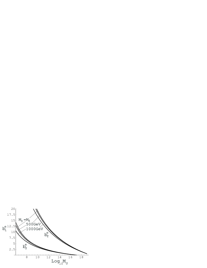
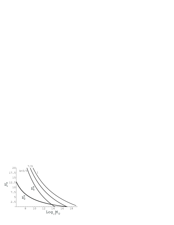
(a)	(b)

Figure 1: The required $b^{e}_{i}$ coefficients from extra matter as a function of the logarithm of the unification scale. (a) The normalisation factor $k=1$ while the three lines for each coupling corresponds to three choices of $M_{0}$ scale, namely: $M_{Z}$, 500 and 1000 GeV. (b) For $M_{0}=500$ GeV, the three lines of the $b^{e}_{Y}$ corresponds to three values of the normalisation factor $k=3/5$, $7/9$ and 1. The thickness of each line corresponds to the experimental error to $\alpha_{3}$ (mainly) and $\sin^{2}\theta$ at the $M_{Z}$.

We point out that the scale $M_{0}$ is not necessarily $M_{Z}$ but the scale where the extra matter start contributing to the running of the gauge couplings. Therefore, $\alpha_{i_{0}}$ is the value at this scale, running from $M_{Z}$ with the SM $b$ coefficients.

In Fig.1(a) we show the relations of Eq.(3) keeping $M_{0}$ as a parameter: i.e. for each chosen scale of unification $M_{U}$ in the $x$-axis, the $y$-axis gives the required $b^{e}_{2}$ and $b^{e}_{Y}$ in order to achieve unification at that scale. In each group the three lines correspond to the values $M_{0}=M_{Z}$, 500GeV and 1TeV. Finally, the thickness of the lines corresponds to the errors of the experimental values of $\alpha_{3}$ (mainly) and $\sin^{2}\theta$ at $M_{Z}$. Since $b^{e}$ comes from matter contribution, it should be positive. Therefore, from the figure we see that the maximum allowed $M_{U}$ is of the order of $10^{17}$ GeV, i.e. when $b^{e}_{2}$ becomes negative. Also Fig.1 shows the obvious result that the lower the unification scale the richer the extra matter content required to achieve unification. Finally, since the running of the strong coupling is unaffected, $U(1)$ needs more matter content to catch up the running of the $SU(2)$ coupling towards the strong one.

Fig.1(b) is similar to Fig.1 but we show the dependence on the $U(1)$ normalisation factor $k$ for the case $M_{0}=500$ GeV. We plot $b^{e}_{2}$ and $b^{e}_{Y}$ for $k=3/5$, $7/9$ and 1 (for comparison). The $k=7/9$ case is chosen since it is a possible value where unification can be achieved with no extra matter. The value $k=3/5$ corresponds of course to the $SU(5)$ normalisation. We also see that, as $k$ is lowered, $b^{e}_{Y}$ dictates the maximum allowed value of $M_{U}$ since it goes to zero quicker than $b^{e}_{2}$. In Fig.2 we present the case of no extra matter by plotting contours of $b^{e}_{2}=b^{e}_{Y}=0$ in the $(\log_{10}M_{U},k)$ plane. The two vertical lines (independent of $k$) defines the strip of $b^{e}_{2}=0$ while the inclined strip corresponds to $b^{e}_{Y}=0$. The horizontal lines show the allowed $k$ values for unification, $(0.764$ - $0.794)$, while the corresponding value for $M_{U}$ is $\sim 10^{16.9-17.2}$ GeV.

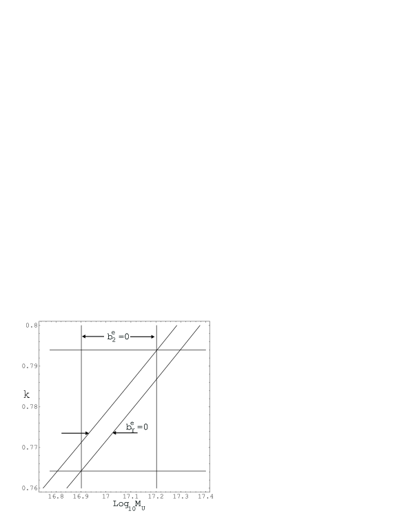
Figure 2: Contours of $b^{e}_{2}=b^{e}_{Y}=0$ on the $(\log_{10}M_{U},k)$ plane.

In Fig.3 we show the relation between $b^{e}_{Y}$ and $b^{e}_{2}$, Eq.(4), for $M_{0}=500$ GeV and for the three values of $k=3/5$, $7/9$ and $1$. We indicate also three values of the unification scale $M_{U}=10^{11}$, $10^{13}$ and $10^{15}$ GeV.

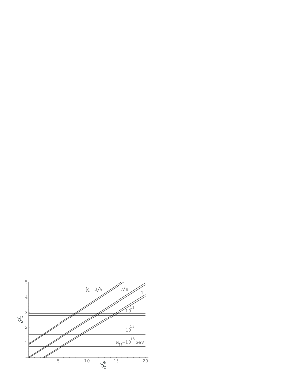
Figure 3: The relation between $b^{e}_{Y}$ and $b^{e}_{2}$ for $M_{0}=500$ GeV and for three values of the normalisation factor $k=3/5$, $7/9$ and $1$. We draw also three lines which correspond to $M_{U}=10^{11}$, $10^{13}$ and $10^{15}$ GeV.

$M_{0}$ (TeV)	$b^{e}_{Y}$	Scalars		Fermions
		No	$Q$	No	$Q$
$k=1$
$M_{Z}\rightarrow$ 0.160	7/3	3	1	2	1
0.450$\rightarrow$12	8/3	0	0	4	1
		2	2	0	0
		1	2	2	1
		4	1	2	1
$k=4/5$
$M_{Z}\rightarrow 500$	4/15	1	1	0	0

Table 1: Regions of scale $M_{0}$ where unification is possible, with $b^{e}_{2}=0$, and the indicated value for $b^{e}_{Y}$ for two values of $k=1$ and $4/5$. The possible combinations of fermions and/or scalars contributing the desired value to $b^{e}_{Y}$ are are also given.

To make the analysis more comprehensive, our next step is to further assume (still with $b^{e}_{3}=0$) that the extra matter content has only $U(1)$ interactions and try to find the multiplicity as well as the integer electric charges (or the $U(1)$ quantum numbers) needed to have unification. In Table 1 we give the regions where unification can be achieved as well as the possible set of extra matter. Of course, always $M_{U}\sim 10^{17}$ GeV since $b^{e}_{2}=0$ and therefore the unification scale is determined by the (MS) running of $\alpha_{3}$ and $\alpha_{2}$. For values of $k$ lower than $4/5$ the minimum value that $b^{e}_{Y}$ could take is larger than the required $b^{e}_{Y}$, and as we have seen in Fig.1(b), the lower the value of $k$ the lower the required $b^{e}_{Y}$ to achieve unification, keeping $b^{e}_{2}=0$.

$b^{e}_{Y}$	$b^{e}_{2}$	Scalars		Fermions		$M_{U}$ (GeV)
		No	$Y$ charge	No	$Y$ charge
$k=1$
37/6	5/6	1	1/2	2	3/2	(2.6-3.0)$10^{14}$
29/3	5/3	6	3/2	2	1/2	(4.7-5.3)$10^{12}$
		2	5/2	4	1/2
79/6	5/2	7	1/2	4	3/2	(2.4-2.6)$10^{11}$
89/6	17/6	9	3/2	4	1/2	(7.5-8.2)$10^{10}$
121/6	25/6	13	1/2	6	3/2	(3.9-4.2)$10^{9}$
71/3	5	14	3/2	8	1/2	(8.9-9.5)$10^{8}$
$k=7/9$
553/4	5/2	7	1/2	4	3/2	(2.3-2.7)$10^{11}$
623/4	17/6	9	3/2	4	1/2	(0.9-1.0)$10^{11}$
413/27	11/3	10	1/2	6	3/2	(0.9-1.0)$10^{10}$
		2	7/2	10	1/2
161/9	13/3	14	3/2	6	1/2	(2.5-2.8)$10^{9}$
553/27	5	14	1/2	8	3/2	(8.5-9.3)$10^{8}$
$k=3/5$
3/5	1	6	1/2	0	0	(0.9-1.0)$10^{14}$
		2	1/2	2	1.2
22/5	2	8	1/2	2	3/2	(1.2-1.5)$10^{12}$
		4	3/2	4	1/2
129/10	25/6	13	3/2	6	1/2	(3.6-4.1)$10^{9}$
91/10	19/6	3	5/2	8	1/2	(3.1-4.7)$10^{10}$
69/5	13/3	14	3/2	6	1/2	(2.3-2.7)$10^{9}$
157/10	29/6	13	1/2	8	3/2	(0.9-1.0)$10^{9}$

Table 2: The required values of $b^{e}_{2}$ and $b^{e}_{Y}$ in order to acheive unification of the couplings, for three values of $k$. We assume that the extra matter forms $SU(2)$ doublets and is colorless. The possible combinations of fermions and scalars with the corresponding Y charges as well as the unification scale are also given. We keep the number of extra multiplets under 15 and $M_{0}=500$ GeV

Now we turn to extra matter that has necessarily both $SU(2)$ and $U(1)$. Although the values that $b^{e}_{1}$ and $b^{e}_{1}$ can take is really great, the number of acceptable cases stays relatively low. For example, assuming that the extra particle, fermion and/or scalars, are in the fundamental representation (doublet) with integer electric charge and allowing up to 14 doublets for each kind, we get 2555 different combinations. Only 7 of them are leading to unification (with $k=1$) if these extra particle starts to contribute at the scale of $M_{0}={\rm 500GeV}$ to the running. In Table 2 we show several combinations of extra particles for two more values of $k$. The unification scale runs from $10^{15}$ GeV down to $10^{8}$ GeV. Of course, the lower the unification scale is the reacher the new spectrum. In Fig.4 we show the possible combinations of $b^{e}_{1}$ and $b^{e}_{2}$ and the ones (inside the band) that lead to unification (for $k=1$).

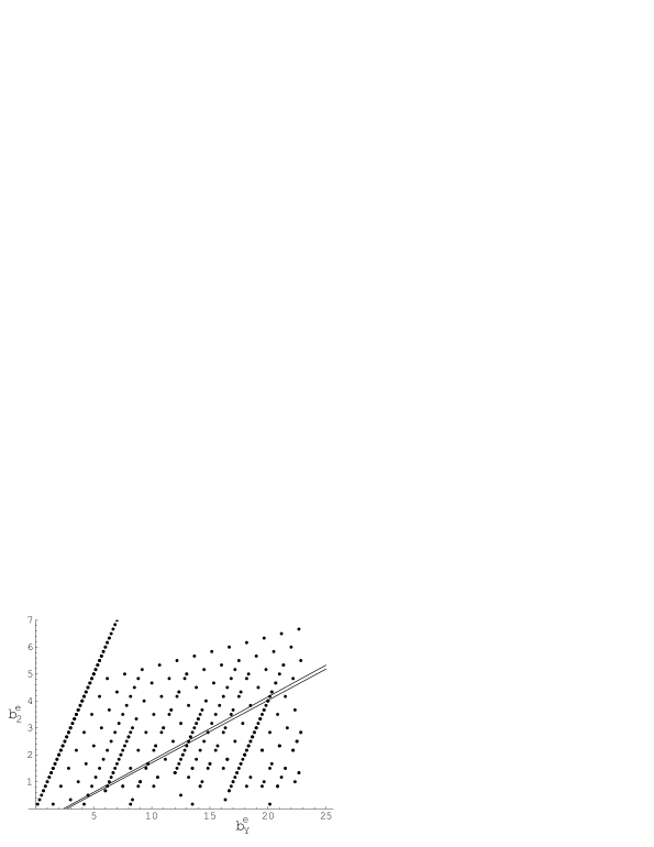
Figure 4: The possible values of $b^{e}_{1}$ and $b^{e}_{2}$ are represented by dots. The band corresponds to $M_{0}=500$ GeV. Only the dots which are inside the band are acceptable for unification ($k=1$).

We can continue trying for higher representations. For example, with just 2 scalar tetraplets with $Y=5/2$ we can achieve unification at the scale $(2.8-3.1)10^{10}$ GeV for $M_{0}=500$ GeV and $(4.2-4.5)10^{10}$ GeV for $M_{0}=1$ TeV.

In our next step we introduce colored extra matter. It consists of one fermion multiplet with quantum numbers $(8,1)_{0}$ under $SU(3)\times SU(2)\times U(1)$. i.e. a gluino-like particle. Of course, the previous values of the $b^{e}_{Y}$ and $b^{e}_{2}$ correspond now to the differences $b^{e}_{Y}-b^{e}_{3}$ and $b^{e}_{2}-b^{e}_{3}$ with $M_{U}$ unchanged. The results are shown in Table 3. The connection between the entries of Table 2 and Table 3 is simple. Since we add a “gluino”, we change $b^{e}_{3}$ by $+2$. Therefore we should change also $b^{e}_{Y}$ and $b^{e}_{2}$ by the same value in order to keep the differences the same. Thus, for $k=1$, we can achieved unification with, for example, 6 extra fermions or 12 extra scalars or 4 fermions and 4 scalars, all doublets under $SU(2)$ with $Y=1/2$. For $k\neq 1$ the required changes in $b^{e}_{2}$ and $b^{e}_{Y}$ lead to small values of $k$ that do not fit to the ones shown in Table2. Nevertheless, some interesting minimal cases appear like the following: With no extra colour particles, an extra $SU(2)$ scalar triplet with $Y=1$ is enough to achieve unification around $10^{15}$ GeV when $k=2/3$. If we assume an extra gluino-like particle, it suffices to add 3 more scalars with the same quantum numbers.

$\delta b^{e}_{Y3}$	$\delta b^{e}_{23}$	Scalars		Fermions		$M_{U}$ (GeV)
		No	$Y$ charge	No	$Y$ charge
37/6	5/6	13	1/2	2	3/2	(2.6-3.0)$10^{14}$
29/3	5/3	6	3/2	8	1/2	(4.9-5.3)$10^{12}$
		2	5/2	10	1/2
71/3	5	14	3/2	14	1/2	(8.9-9.5)$10^{8}$

Table 3: The required values of the differences $b^{e}_{2}-b^{e}_{3}$ and $b^{e}_{Y}-b^{e}_{3}$ in order to acheive unification of the couplings. The extra colored matter consists of one fermion multiplet with quantum numbers $(8,1)_{0}$ under $SU(3)\times SU(2)\times U(1)$ while the extra non colored matter consists of $SU(2)$ doublets. The possible combinations of fermions and scalars of the non colored matter with the corresponding Y charges as well as the unification scale are also given. We keep the number of extra multiplets under 15, $M_{0}=500$ GeV and $k=1$.

Let us now consider a case which resembles the split supersymmetry one, i.e. the extra matter contains one $(8,1)_{0}$ (gluino-like), one $(1,3)_{0}$ (wino-like) and two $(1,2)_{1}$ (higgsinos-like). The question is what extra matter, apart from those, are needed to achieve unification. If we admit $U(1)$ only charged extra matter (and $k=1$), with $M_{0}=500$ GeV, we need 3 scalars with $Y=3$ and 2 fermions with $Y=1$. If we choose $M_{0}=1$ TeV, there are numerous solutions but the minimal one consists of four fermions with $Y=2$. In both cases $M_{U}\sim 10^{13}$ GeV. If the extra matter (again beyond the gluino-, wino- and higgsino-like) falls in the fundamental representation of $SU(2)$, then the most economical solution (again with $k=1$) is two scalars with $Y=1/2$ and two fermions with $Y=3/2$. The unification scale is $\sim 10^{14}$ GeV. If the extra matter falls in the triplet of $SU(2)$, one scalar with $Y=4$ and two more wino-like multiplets are enough to lead to unification at $M_{U}\sim 2\times 10^{10}$ GeV.

3 SO(10) Unification

There are various symmetry breaking patterns for $SO(10)$[11] leading to an intermediate group $G\subset SO(10)$, which subsequently it further breaks to $SU(3)\times SU(2)\times U_{Y}(1)\subset G$. The various possibilities for $G$ include (i) $G=SU(5)$, (ii) the Pati-Salam $G=SU(4)\times SU(2)\times SU(2)$ (iii) the flipped $G=SU(5)\times U(1)$, iv)$G=SU(3)\times U(1)\times SU(2)\times SU(2)$ e.tc. Here we will consider the cases of the Pati-Salam and flipped $SU(5)$ (ii) and (iii), respectively.

The Pati-Salam $SU(4)\times SU(2)_{L}\times SU(2)_{R}$ GUT model

We will consider here the possibility of unification through the Pati-Salam GUT model $SU(4)\times SU(2)_{L}\times SU(2)_{R}$. The scalar sector contains a 210, a 126 and a 10 of $SO(10)$. The 210 breaks $SO(10)\to SU(4)\times SU(2)_{L}\times SU(2)_{R}$, the 126 breaks $SU(4)\times SU(2)_{L}\times SU(2)_{R}$ to $SU(3)_{C}\times SU(2)_{L}\times U(1)_{R}\times U(1)_{C}$, whereas the 10 further breaks to the SM group $SU(3)_{C}\times SU(2)\times U(1)_{Y}$. The symmetry pattern is then

$$\begin{split}SO(10)\!\stackrel{{\scriptstyle 210}}{{\longrightarrow}}\!SU(4)\!\times\!SU(2)_{L}\!\times\!SU(2)_{R}&\stackrel{{\scriptstyle 126}}{{\longrightarrow}}SU(3)_{C}\!\times\!SU(2)_{L}\times\!U(1)_{R}\!\times\!U(1)_{C}\stackrel{{\scriptstyle 10}}{{\longrightarrow}}\\ SU(3)_{C}\!\times\!S&U(2)\!\times\!U(1)_{Y}\end{split}$$

At the GUT scale we have the relation:

$$\alpha_{4}=\alpha_{3},\quad\alpha_{2L}=\alpha_{2},\quad\alpha_{Y}^{-1}=3/5\,\alpha_{2R}^{-1}+2/5\,\alpha_{4}^{-1}$$ (5)

while the $U(1)_{Y}$ quantum numbers are related to the corresponding ones in $SU(4)$ and $SU(2)_{R}$ through the relation:

$$Y=\sqrt{3/5}\,Y_{2R}+\sqrt{2/5}\,Y_{4}$$ (6)

The SM particles (quarks and leptons plus a right handed neutrino) are in the $(4,2,1)$ and $(\bar{4},1,2)$ representations of $SU(4)\times SU(2)_{L}\times SU(2)_{R}$ (these two multiplets make the 16 representation of $SO(10)$). The required Higgs to break the Pati-Salam group down to the SM are in the $(\bar{10},1,3)$ representations while the SM Higgs is in the $(1,2,2)$ representation.

The energy scales we are using are the following:

• $M_{U}$, where $\alpha_{4}=\alpha_{2L}=\alpha_{2R}$,

• $M_{G}$, where the Pati-Salam model breaks to the SM. In the region between $M_{U}$ and $M_{G}$ we have the minimal content of the Pati-Salam group consisting of SM particles in $(4,2,1)$ and $(\bar{4},1,2)$, Higgs fields in $(\bar{10},1,3)$ and $(1,2,2)$ plus some extra fermionic matter,

• Below $M_{G}$, down to some scale $M_{N}$, we have the SM particles in $(4,2,1)$ and the $(\bar{4},1,2)$, $(1,2,2)$ Higgs, plus some extra fermionic matter and

• Below $M_{N}$ we have only the SM content.

We assume that all extra fermionic matter come from the 10, 16 and 45 representations of $SO(10)$. We have 16 cases which are shown in Table 4. In each case, the first line gives the quantum numbers under the corresponding group. The second line gives the contribution to the SM $\beta$-functions and to the Pati-Salam model for one multiplet.

$$\begin{array}[]{|c|ccc|}\hline\cr CASE&SU(3)\times SU(2)\times U(1)_{Y}&SU(4)\times SU(2)_{L}\times SU(2)_{R}&SO(10)\\ \hline\cr 1&\mathbf{(3,1,\sqrt{4/15})}&\mathbf{(4,1,2)}&\mathbf{16}\\ &(b_{3},b_{2},b_{1})=(1/3,0,8/15)&(b_{4},b_{2L},b_{2R})=(2/3,0,4/3)&\\ \hline\cr 2&\mathbf{(3,1,-\sqrt{1/15})}&\mathbf{(4,1,2)}&\mathbf{16}\\ &(1/3,0,2/15&(2/3,0,4/3)&\\ \hline\cr 3&\mathbf{(\stackrel{{\scriptstyle(-)}}{{3}},1,\mp\sqrt{1/15})}&\mathbf{(6,1,1)}&\mathbf{10}\\ &(1/3,0,2/15)&(2/3,0,0)&\\ \hline\cr 4&\mathbf{(\stackrel{{\scriptstyle(-)}}{{3}},1,\pm\sqrt{2/15})}&\mathbf{(15,1,1)}&\mathbf{45}\\ &(1/3,0,4/15)&(8/3,0,0)&\\ \hline\cr 5&\mathbf{(\stackrel{{\scriptstyle(-)}}{{3}},2,\pm\sqrt{1/60})}&\mathbf{(6,2,2)}&\mathbf{45}\\ &(2/3,1,1/15)&(8/3,4,4)&\\ \hline\cr 6&\mathbf{(\stackrel{{\scriptstyle(-)}}{{3}},1,\pm 5\sqrt{60})}&\mathbf{(6,2,2)}&\mathbf{45}\\ &(2/3,1,5/3)&(8/3,4,4)&\\ \hline\cr 7&\mathbf{(1,1,\pm\sqrt{3/5})}&\mathbf{(1,1,3)}&\mathbf{45}\\ &(0,0,2/5)&(0,0,4/3)&\\ \hline\cr 8&\mathbf{(1,3,0)}&\mathbf{(1,3,1)}&\mathbf{45}\\ &(0,4/3,0)&(0,4/3,0)&\\ \hline\cr 9&\mathbf{(8,1,0)}&\mathbf{(15,1,1)}&\mathbf{45}\\ &(2,0,0)&(8/3,0,0)&\\ \hline\cr 10&\mathbf{(1,1,0)}&\mathbf{(15,1,1)}&\mathbf{45}\\ &(0,0,0)&(8/3,0,0)&\\ \hline\cr 11&\mathbf{(1,1,0)}&\mathbf{(4,1,2)}&\mathbf{16}\\ &(0,0,0)&(2/3,0,4/3)&\\ \hline\cr 12&\mathbf{(1,1,0)}&\mathbf{(1,1,3)}&\mathbf{45}\\ &(0,0,0)&(0,0,4/3)&\\ \hline\cr 13&\mathbf{(1,2,\pm\sqrt{3/20})}&\mathbf{(1,2,2)}&\mathbf{10}\\ &(0,1/3,1/5)&(0,1/3,1/3)&\\ \hline\cr 14&\mathbf{(\bar{3},2,-\sqrt{1/60})}&\mathbf{(\bar{4},2,1)}&\mathbf{16}\\ &(2/3,1,1/15)&(2/3,4/3,0)&\\ \hline\cr 15&\mathbf{(1,2,\sqrt{3/20})}&\mathbf{(\bar{4},2,1)}&\mathbf{16}\\ &(0,1/3,1/5)&(2/3,4/3,0)&\\ \hline\cr 16&\mathbf{(1,1,-\sqrt{3/5})}&\mathbf{(4,1,2)}&\mathbf{16}\\ &(0,0,2/5)&(2/3,0,4/3)&\\ \hline\cr\end{array}$$

Table 4: The 16 possible cases of $SU(4)\times SU(2)_{L}\times SU(2)_{R}$ which fall in the 10, 16 and 45 multiplets of $SO(10)$. The corresponding contribution to the $\beta$-functions are also given for each case in the second line.

The number of free parameters are great: $M_{N}$, $M_{G}$ and the number of each multiplet. We are going to limit this parameter space, choosing first, to make the running independent of the scale $M_{N}$. This could happen if the contribution of the extra matter to the SM $\beta$-functions are equal (since the unification depends only on the differences of the contributions). For example, if the contribution to the SM $\beta$-function coefficients from extra matter is 2/3, choosing $M_{G}\sim 6.3\times 10^{6}$ GeV, we can achieve unification at $M_{U}\sim 4\times 10^{17}$ GeV . A minimal extra matter content for that case is 2 multiplets from case 2 and from case 13 of Table 4. Notice that in this standard (non-SUSY) version of the PS model, we are safe against proton decay and we should only take care of a high $M_{U}$ energy scale [11].

Another idea that we have checked is the possibility that $M_{N}=M_{G}$, i.e. the extra matter is only in the energy region of the Pati-Salam model (not requiring necessarily equality of SM extra contributions). We have found that if $M_{N}=M_{G}=1$ TeV we can achieve unification at $M_{U}\sim 5\times 10^{17}$ GeV. In Table 5 we show the lowest possible extra content in the region between $M_{G}$ and $M_{U}$. In Fig.5 we plot the corresponding running of the couplings. If we rase the 1 TeV scale to 5 TeV, then we get unification at $M_{U}\sim 6\times 10^{14}$ GeV.

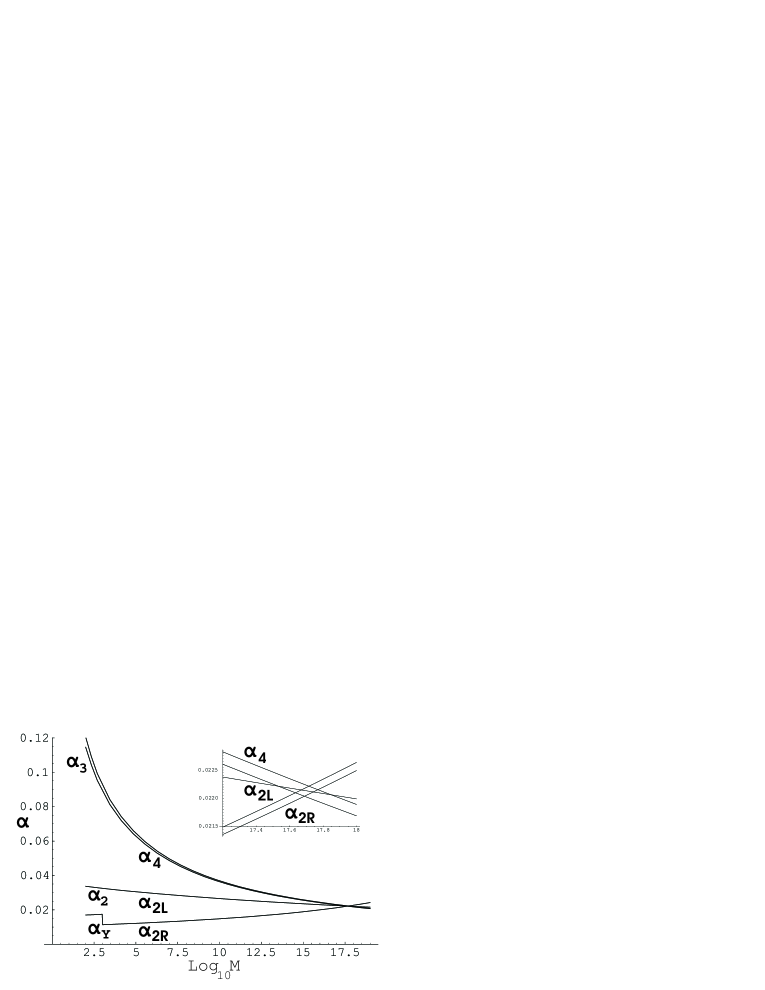
Figure 5: The coupling running for the PS model. $M_{N}=M_{G}=1$ GeV. The extra content above $M_{G}$ is 2 multiplets from case 2, 1 from case 7 and 1 from case 13 of Table 5.

$$\begin{array}[]{|c|c|c|c|c|c|c|c|}\hline\cr(4,1,2)&(6,1,1)&(15,1,1)&(6,2,2)&(1,1,3)&(1,3,1)&(1,2,2)&(\bar{4},2,1)\\ \hline\cr 2&0&0&0&1&0&1&0\\ \hline\cr\end{array}$$

Table 5: The lowest possible combinations of Pati-Salam multiplets for $M_{N}=M_{G}=1$ TeV and $M_{U}\sim 5\times 10^{17}$ GeV.

The flipped $SU(5)$ GUT model
The $SU(5)\times U(1)$ group is another possible GUT model, subgroup of $SO(10)$. At the GUT scale we have the relations:

$$\alpha_{5}=\alpha_{3}=\alpha_{2},\quad\alpha_{Y}^{-1}=1/25\,\alpha_{5}^{-1}+24/25\,\alpha_{1}^{-1}$$ (7)

The $U(1)_{Y}$ quantum numbers are related to the corresponding $U(1)$’s in $SU(5)$ and the $U(1)$ by the relation

$$Y=-\frac{1}{5}\,Y_{5}+\frac{\sqrt{24}}{5}\,Y_{1}$$ (8)

The matter content lie in the 5^∗, 10 and 1 of $SU(5)$ (again these three multiplets make the 16 of $SO(10)$) and the higgs are in the 10 and 5^∗. We allow extra matter (either in $SU(5)\times U(1)$ or in the SM region) that can be found in the 10, 16 and 45 of $SO(10)$. There are 12 cases shown in Table 6.

$$\begin{array}[]{|c|ccc|}\hline\cr CASE&SU(3)\times SU(2)\times U(1)_{Y}&SU(5)\times U(1)&SO(10)\\ \hline\cr 1&\mathbf{(3,1,-\sqrt{1/15})}&\mathbf{(5,-\sqrt{1/10})}&\mathbf{10}\\ &(b_{3},b_{2},b_{Y})=(1/3,0,2/15)&(b_{5},b_{1})=(1/3,1/3)&\\ \hline\cr 2&\mathbf{(3,1,-\sqrt{1/15})}&\mathbf{(10,\sqrt{1/40})}&\mathbf{16}\\ &(1/3,0,2/15)&(1,1/6)&\\ \hline\cr 3&\mathbf{(1,2,-\sqrt{3/20})}&\mathbf{(5,-\sqrt{1/10})}&\mathbf{10}\\ &(0,1/3,1/5)&(1/3,1/3)&\\ \hline\cr 4&\mathbf{(1,2,-\sqrt{3/20})}&\mathbf{(\stackrel{{\scriptstyle-}}{{5}},-\sqrt{9/40})}&\mathbf{16}\\ &(0,1/3,1/5)&(1/3,3/4)&\\ \hline\cr 5&\mathbf{(3,2,\sqrt{1/60})}&\mathbf{(10,\sqrt{1/40})}&\mathbf{16}\\ &(2/3,1,1/15)&(1,1/6)&\\ \hline\cr 6&\mathbf{(3,2,\sqrt{1/60})}&\mathbf{(24,0)}&\mathbf{45}\\ &(2/3,1,1/15)&(10/3,0)&\\ \hline\cr 7&\mathbf{(\stackrel{{\scriptstyle-}}{{3}},1,-\sqrt{4/15})}&\mathbf{(\stackrel{{\scriptstyle-}}{{5}},-\sqrt{9/40})}&\mathbf{16}\\ &(1/3,0,8/15)&(1/3,3/4)&\\ \hline\cr 8&\mathbf{(\stackrel{{\scriptstyle-}}{{3}},1,-\sqrt{4/15})}&\mathbf{(10,-\sqrt{2/5})}&\mathbf{45}\\ &(1/3,0,8/15)&(1,8/3)&\\ \hline\cr 9&\mathbf{(1,1,\sqrt{3/5})}&\mathbf{(1,\sqrt{5/8})}&\mathbf{16}\\ &(0,0,2/5)&(0,5/12)&\\ \hline\cr 10&\mathbf{(1,1,\sqrt{3/5})}&\mathbf{(10,-\sqrt{2/5})}&\mathbf{45}\\ &(0,0,2/5)&(1,8/3)&\\ \hline\cr 11&\mathbf{(8,1,0)}&\mathbf{(24,0)}&\mathbf{45}\\ &(2,0,0)&(10/3,0)&\\ \hline\cr 12&\mathbf{(3,2,\sqrt{5/12})}&\mathbf{(10,-\sqrt{2/5})}&\mathbf{45}\\ &(2/3,1,5/3)&(1,8/3)&\\ \hline\cr 13&\mathbf{(1,1,0)}&\mathbf{(10,\sqrt{1/40})}&\mathbf{16}\\ &(0,0,0)&(1,1/6)&\\ \hline\cr 14&\mathbf{(1,1,0)}&\mathbf{(24,0)}&\mathbf{45}\\ &(0,0,0)&(10/3,0)&\\ \hline\cr\end{array}$$

Table 6: The 14 possible cases of $SU(5)\times U(1)$ which fall in the 10, 16 and 45 multiplets of $SO(10)$. The corresponding contribution to the $\beta$-functions are also given.

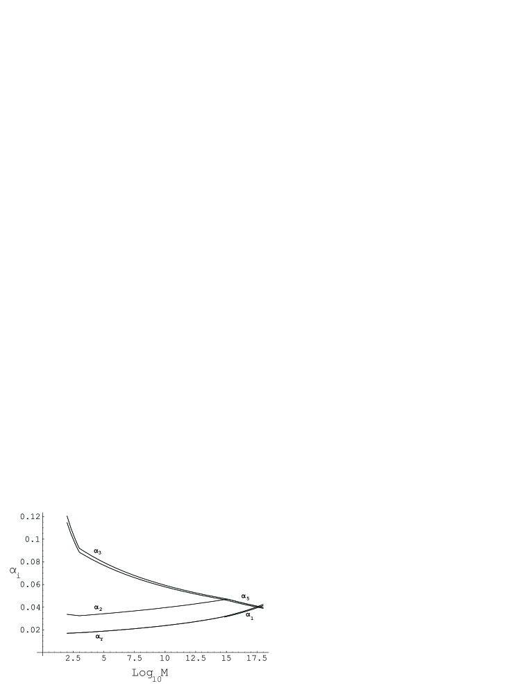
Figure 6: The coupling runnings for the flipped $SU(5)$ model. The new SM multiplets appear at the 1 TeV scale. For the specific choice of extra multiplets, (0,0,2,2,2,2,0,0,2,0,1,0,0,0), $M_{G}\sim 10^{15}$ GeV while $M_{U}\sim 4\,10^{17}$ GeV.

In this model the grand unification scale $M_{G}$ is where the $SU(3)$ and the $SU(2)$ couplings meet. Then the couplings of $SU(5)$ and $U(1)$ run and their meeting point indicates the unification scale $M_{U}$. Asking the number of extra multiplets for each case to be at most 2 (the lowest possible value), and requiring that $M_{G}\geq 10^{14}$ GeV (to avoid fast proton decay) and $M_{U}\leq 10^{18}$ GeV, we get numerous solutions. However, they all fall in two categories: (i) both $M_{G}$ and $M_{U}$ are in the scale of $10^{17}$ GeV and (ii) $M_{G}\sim(0.7-1)10^{15}$ GeV and $M_{U}$ could be either $(0.2-4)10^{16}$ GeV or $(2-4)10^{17}$ GeV. In Fig. 6 we show the running of the couplings for the case (0,0,2,2,2,2,0,0,2,0,1,0,0,0), where the numbers correspond to the number of species from each of the fourteen cases in Table 6. We have assumed, as before, that the extra SM multiplets appear at the scale of 1 TeV.

4 Conclusions

We had performed a wide (1-loop analysis) answering the question: “How much and what kind of extra matter should we add to the SM content to achieve unification?”. Forgetting, in the first step, any covering group, we found numerous solutions with $U(1)$ only charged extra matter (therefore the unification scale stays in the order of $M_{U}=10^{16}$ GeV), or with $SU(2)$ charged extra matter ($M_{U}$ starts to get lower) as well as for the case of gluino-like extra matter. We also examine the case of various $U(1)_{Y}$ normalisations as it happens in GUT theories on orbifolds [12] and in their deconstructions [13] and D-brane derived models [14]. This corresponds to unification of the SM into a more fundamental theory, like string theory, without any GUT intermediate step. Such gauge coupling unification has been considered before [15], [16],[17],[18] Then we have identified the SM extra matter as coming from the breaking of $SO(10)$ [11],[19] either through the Pati-Salam group $SU(4)\times SU(2)_{L}\times SU(2)_{R}$ or flipped $SU(5)$. We have not discussed some other breaking of $SO(10)$, which are triggered by Higgs scalars in other $SO(10)$ representations [20]. For both cases we present, unification can be achieved by a rather minimal extra content. This is reminiscent of the work in [2], where however, a one-step unification has been followed and the $SU(3)\times SU(2)\times U_{Y}(1)$ is unified to $SU(5)$. In this case, proton stability requires the existence of coloured particles in the electroweak scale. These particles, if stable, could be bound on nuclei, giving rise to anomalous heavy isotopes. There are various searches of such heavy isotopes using deep sea water, which put bounds on the concentration of stable charged particles of less than $10^{17}$ for mass up to $1600~{}m_{p}$ [21]. However, in the case of a two-step unification, i.e., in the case of an $SO(10)$ unification with a partial intermediate unification of Pati-Salam or flipped $SU(5)$ unification, unification may achieved without introducing necessarily coloured particles. In both cases, there are stable dark matter candidates, while the splitting of irreps (the double-triplet splitting in the case of $SU(5)$) is the same for both one-step and two-step unification.

The project is co - funded by the European Social Fund (75%) and National Resources (25%) - (EPEAEK II) -PYTHAGORAS. The work of NDT is partially supported by the MRTN-CT-2004-503369 European Network.

References

- [1] N. Arkani-Hamed and S. Dimopoulos, arXiv:hep-th/0405159.
- [2] G. F. Giudice and A. Romanino, Nucl. Phys. B 699, 65 (2004) [Erratum-ibid. B 706, 65 (2005)] [arXiv:hep-ph/0406088].
- [3] N. Arkani-Hamed, S. Dimopoulos, G. F. Giudice and A. Romanino, Nucl. Phys. B 709, 3 (2005) [arXiv:hep-ph/0409232].
- [4] I. Antoniadis and S. Dimopoulos, Nucl. Phys. B 715, 120 (2005) [arXiv:hep-th/0411032].
- [5] B. Kors and P. Nath, Nucl. Phys. B 711, 112 (2005) [arXiv:hep-th/0411201].
- [6] J. C. Pati and A. Salam, Phys. Rev. D 10, 275 (1974).
- [7] S. M. Barr, Phys. Lett. B 112, 219 (1982).
- [8] J. P. Derendinger, J. E. Kim and D. V. Nanopoulos, Phys. Lett. B 139, 170 (1984).
- [9] I. Antoniadis, J. R. Ellis, J. S. Hagelin and D. V. Nanopoulos, Phys. Lett. B 194, 231 (1987).
- [10] P. Q. Hung, Phys. Rev. Lett. 80, 3000 (1998) [arXiv:hep-ph/9712338].
- [11] D. G. Lee, R. N. Mohapatra, M. K. Parida and M. Rani, Phys. Rev. D 51, 229 (1995) [arXiv:hep-ph/9404238].
- [12] Y. Kawamura, Prog. Theor. Phys. 103, 613 (2000); G. Altarelli and F. Feruglio, Phys. Lett. B 511, 257 (2001); L. Hall and Y. Nomura, Phys. Rev. D 64, 055003 (2001); A. Hebecker and J. March-Russell, Nucl. Phys. B 613, 3 (2001); T. Li, Phys. Lett. B 520, 377 (2001); Nucl. Phys. B 633, 83 (2002)
- [13] N. Arkani-Hamed, A. G. Cohen and H. Georgi, Phys. Rev. Lett. 86, 4757 (2001); C. T. Hill, S. Pokorski and J. Wang, Phys. Rev. D 64, 105005 (2001).
- [14] R. Blumenhagen, M. Cvetic, P. Langacker and G. Shiu, arXiv:hep-th/0502005.
- [15] J.A. Casas and C. Munoz, Phys. Lett. B 214 543 (1988).
- [16] L. E. Ibanez, Phys. Lett. B 318, 73 (1993) [arXiv:hep-ph/9308365].
- [17] K. R. Dienes, Phys. Rept. 287, 447 (1997) [arXiv:hep-th/9602045].
- [18] V. Barger, J. Jiang, P. Langacker and T. Li, arXiv:hep-ph/0503226.
- [19] X. Calmet, Eur. Phys. J. C 41, 245 (2005) [arXiv:hep-ph/0406314].
- [20] G. Lazarides, M. Magg and Q. Shafi, Phys. Lett. B 97, 87 (1980); D. Chang and A. Kumar, Phys. Rev. D 33, 2695 (1986); X. G. He and S. Meljanac, Phys. Rev. D 40, 2098 (1989); J. Basecq, S. Meljanac and L. O’Raifeartaigh, Phys. Rev. D 39, 3110 (1989); O. Kaymakcalan, L. Michel, K. C. Wali, W. D. McGlinn and L. O’Raifeartaigh, Nucl. Phys. B 267, 203 (1986).
- [21] T. Yamagata, Y. Takamori, and H. Utsunomiya, Phys. Rev. D 47, 1231 (1993).
- [22] D. Javorsek, D. Elmore1, E. Fischbach1, D. Granger, T. Miller, D. Oliver, and V. Teplitz, Phys. Rev. Lett. 87, 231804 (2001).