Factorization in the Production and Decay of the $X(3872)$

Abstract

The production and decay of the $X(3872)$ are analyzed under the assumption that the $X$ is a weakly-bound molecule of the charm mesons $D^{0}\bar{D}^{*0}$ and $D^{*0}\bar{D}^{0}$. The decays imply that the large $D^{0}\bar{D}^{*0}$ scattering length has an imaginary part. An effective field theory for particles with a large complex scattering length is used to derive factorization formulas for production rates and decay rates of $X$. If a partial width is calculated in a model with a particular value of the binding energy, the factorization formula can be used to extrapolate to other values of the binding energy and to take into account the width of the $X$. The factorization formulas relate the rates for production of $X$ to those for production of $D^{0}\bar{D}^{*0}$ and $D^{*0}\bar{D}^{0}$ near threshold. They also imply that the line shape of $X$ differs significantly from that of a Breit-Wigner resonance.

I Introduction

The $X(3872)$ is a narrow resonance near $3872$ MeV discovered by the Belle collaboration in 2003 Choi:2003ue . It has been observed through the exclusive decay $B^{\pm}\to XK^{\pm}$ Choi:2003ue ; Aubert:2004ns and through its inclusive production in proton-antiproton collisions Acosta:2003zx ; Abazov:2004kp . Its mass $m_{X}$ is extremely close to the threshold for the charm mesons $D^{0}$ and $\bar{D}^{*0}$ Olsen:2004fp :

$$m_{X}-(m_{D^{0}}+m_{D^{*0}})=+0.6\pm 1.1\;{\rm MeV}.$$ (1)

The upper bound on its decay width $\Gamma_{X}$ is Choi:2003ue

$$\Gamma_{X}<2.3\;{\rm MeV}\;\;\;{\rm(90\%\;C.L.)}.$$ (2)

The $X(3872)$ was discovered through its decay into $J/\psi\,\pi^{+}\pi^{-}$ Choi:2003ue . The Belle collaboration has recently presented evidence for the decays $X\rightarrow J/\psi\,\pi^{+}\pi^{-}\pi^{0}$ and $X\to J/\psi\,\gamma$ Abe:2005ix . The decay $X\to J/\psi\,\gamma$ implies that the $X$ has positive charge conjugation. Upper bounds have been set on several other decay modes Abe:2003zv ; Yuan:2003yz ; Aubert:2004fc ; Abe:2004sd ; Metreveli:2004px .

The nature of the $X(3872)$ has not yet been definitively established. The presence of the $J/\psi$ among its decay products motivates its interpretation as a charmonium state with constituents $c\bar{c}$ Barnes:2003vb ; Eichten:2004uh ; Quigg:2004nv . Two interpretations that are motivated by the proximity of $m_{X}$ to the $D^{0}\bar{D}^{*0}$ threshold are a hadronic molecule with constituents $DD^{*}$ Tornqvist:2003na ; Tornqvist:2004qy ; Voloshin:2003nt ; Wong:2003xk ; Braaten:2003he ; Swanson:2003tb ; Swanson:2004pp and a “cusp” associated with the $D^{0}\bar{D}^{*0}$ threshold Bugg:2004rk ; Bugg:2004sh . Other proposed interpretations include a tetraquark with constituents $c\bar{c}q\bar{q}$ Vijande:2004vt , a “hybrid charmonium” state with constituents $c\bar{c}g$ Close:2003mb ; Li:2004st , a glueball with constitutents $ggg$ Seth:2004zb , and a diquark-antidiquark bound state with constituents $cu+\bar{c}\bar{u}$ Maiani:2004vq . Measurements of the decays of the $X$ can be used to determine its quantum numbers and narrow down the options Close:2003sg ; Pakvasa:2003ea ; Rosner:2004ac ; Kim:2004cz ; Abe:2005iy . The most predictive of the proposed interpretations are charmonium and $DD^{*}$ molecules. The $C=-$ charmonium options are ruled out by the decay $X\to J/\psi\,\gamma$. Evidence ruling out or disfavoring each of the $C=+$ charmonium options has been accumulating Olsen:2004fp ; Quigg:2004vf ; Abe:2005iy . The most difficult charmonium state to rule out is the $\chi_{c1}(2P)$, partly because it can have resonant S-wave interactions with $D^{0}\bar{D}^{*0}$ and $D^{*0}\bar{D}^{0}$ that transform it into a $DD^{*}$ molecule Braaten:2003he .

The possibility that charm mesons might form molecular states was considered shortly after the discovery of charm Bander:1975fb ; Voloshin:ap ; DeRujula:1976qd ; Nussinov:1976fg . The first quantitative study of the possibility of molecular states of charm mesons was carried out by Tornqvist in 1993 using a one-pion-exchange potential model. He found that the isospin-0 combinations of $D\bar{D}^{*}$ and $D^{*}\bar{D}$ could form weakly-bound states in the S-wave $1^{++}$ channel and in the P-wave $0^{-+}$ channel Tornqvist:1993ng . Since the binding energy is small compared to the 8.4 MeV splitting between the $D^{0}\bar{D}^{*0}$ threshold and the $D^{+}D^{*-}$ threshold, there are large isospin breaking effects Tornqvist:2003na ; Tornqvist:2004qy . After the discovery of the $X(3872)$, Swanson considered a potential model that includes both one-pion-exchange and quark exchange, and found that the $C=+$ superposition of $D^{0}\bar{D}^{*0}$ and $D^{*0}\bar{D}^{0}$ could form a weakly-bound state in the S-wave $1^{++}$ channel Swanson:2003tb . Another mechanism for generating a $DD^{*}$ molecule is the accidental fine-tuning of the mass of the $\chi_{c1}(2P)$ to the $D^{0}\bar{D}^{*0}$/$D^{*0}\bar{D}^{0}$ threshold which creates a $DD^{*}$ molecule with quantum numbers $1^{++}$ Braaten:2003he .

The assumption that the $X(3872)$ is a weakly-bound $DD^{*}$ molecule is very predictive Braaten:2003he . This assumption has been used by Voloshin to predict the rates and momentum distributions for the decays of $X$ into $D^{0}\bar{D}^{0}\pi^{0}$ and $D^{0}\bar{D}^{0}\gamma$ Voloshin:2003nt . It has been used to calculate the rate for the exclusive decay of $\Upsilon(4S)$ into the $X$ and two light hadrons Braaten:2004rw , to estimate the decay rate for the discovery mode $B^{+}\to XK^{+}$ Braaten:2004fk , and to predict the suppression of the decay rate for $B^{0}\to XK^{0}$ Braaten:2004ai . The assumption that the $X$ is a weakly-bound $DD^{*}$ molecule also has implications for inclusive production Braaten:2004jg ; Voloshin:2004mh .

In this paper, we point out that if $X$ is a loosely-bound molecule, its short-distance decay rates and its exclusive production rates satisfy simple factorization formulas. In Section II, we illustrate the factorization formulas using a two-channel scattering model. In Section III, we show how the rate for a short-distance decay mode of the $X$, such as $J/\psi\,\pi^{+}\pi^{-}\pi^{0}$, can be factorized into long-distance factor that involves the large scattering length and a short-distance factor that is insenstitive to $a$. In Section IV, we show how a production rate for the $X$, such as the decay rate for $B^{+}\to XK^{+}$, can be factorized into a long-distance factor and a short-distance factor. In Section V, we use factorization to calculate the shapes of the invariant mass distributions of $D^{0}\bar{D}^{*0}$ and $D^{*0}\bar{D}^{0}$ near threshold. In Section VI, we use factorization to calculate the line shape of the $X$ in any of its short-distance decay modes. The line shape depends on the real and imaginary parts of the scattering length and can differ substantially from a conventional Breit-Wigner resonance. A summary of our results is given in Section VII.

II Factorization in a Simple Scattering Model

II.1 Universality for large scattering length

Nonrelativistic few-body systems with short-range interactions and a large scattering length $a$ have universal properties that depend on the scattering length but are otherwise insensitive to details at distances small compared to $a$ Braaten:2004rn . In any specific system, there is a natural momentum scale $\Lambda$ that sets the scale of most low-energy scattering parameters. The scattering length is large if it satisfies $|a|\gg\Lambda^{-1}$. Universality predicts that the T-matrix element for 2-body elastic scattering with relative momentum $p\ll\Lambda$ is

$${\cal T}(p)={2\pi/\mu\over-1/a-ip},$$ (3)

where $\mu$ is the reduced mass of the two particles. If $a$ is real and positive, universality predicts that there is a weakly-bound state with binding energy

$$E_{X}=\frac{1}{2\mu a^{2}}.$$ (4)

The universal momentum-space wavefunction of this bound state is

$$\psi(p)=\frac{(8\pi/a)^{1/2}}{p^{2}+1/a^{2}}.$$ (5)

The universal amplitude for transitions from the bound state to a scattering state consisting of two particles with relative momentum $p\ll\Lambda$ is

$${\cal A}_{X}={\sqrt{2\pi}\over\mu}\,a^{-1/2}.$$ (6)

These results are all encoded in the universal expression for the truncated connected transition amplitude:

$${\cal A}(E)={2\pi/\mu\over-1/a+\sqrt{-2\mu E}}.$$ (7)

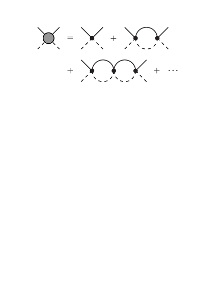
Figure 1: The geometric series of Feynman diagrams whose sum is the universal amplitude ${\cal A}(E)$.

The universal amplitude in Eq. (7) can be obtained from a local effective field theory for the two particles. The particles interact through an S-wave contact interaction with Feynman rule $-i(2\pi/\mu)a_{0}(\Lambda)$, where the parameter $a_{0}(\Lambda)$ is a bare scattering length that depends on the ultraviolet momentum cutoff $\Lambda$. The amplitude ${\cal A}(E)$ can be obtained by summing the geometric series of Feynman diagrams in Fig. 1:

$${\cal A}(E)=-{(2\pi/\mu)a_{0}(\Lambda)\over 1+(2\pi/\mu)a_{0}(\Lambda)L(\Lambda,E)},$$ (8)

where $L(\Lambda,E)$ is the amplitude for the propagation of the particles between successive contact interactions:

$$L(\Lambda,E)={\mu\over\pi^{2}}\left(\Lambda-{\pi\over 2}\sqrt{-2\mu E}\right).$$ (9)

Renormalization is accomplished by eliminating $a_{0}(\Lambda)$ in favor of the physical scattering length:

$$a={a_{0}(\Lambda)\over 1+(2/\pi)\Lambda a_{0}(\Lambda)}.$$ (10)

With this substitution, the expression for ${\cal A}(E)$ in Eq. (8) reduces without approximation to the universal result in Eq. (7). Note that the scattering length $a$ can be tuned to $\pm\infty$ by tuning the bare scattering length to a critical value of order $\Lambda^{-1}$:

$$a_{0}(\Lambda)\longrightarrow-{\pi\over 2}\Lambda^{-1}.$$ (11)

If the 2-body system has inelastic scattering channels, the large scattering length $a$ will have a negative imaginary part. It is convenient to express the complex scattering length in the form

$$\frac{1}{a}=\gamma_{\rm re}+i\gamma_{\rm im},$$ (12)

where $\gamma_{\rm re}$ and $\gamma_{\rm im}$ are real and $\gamma_{\rm im}\geq 0$. In the case $\gamma_{\rm re}>0$ where there is a weakly-bound state, it can decay into the inelastic channel. The expression for the binding energy on the right side of Eq. (4) is complex-valued. Its real part $E_{X,{\rm pole}}$ and its imaginary part $\Gamma_{X}/2$ are given by

$$E_{X,{\rm pole}} = (\gamma_{\rm re}^{2}-\gamma_{\rm im}^{2})/(2\mu),$$ (13a)

$$\Gamma_{X} = 2\gamma_{\rm re}\gamma_{\rm im}/\mu.$$ (13b)

These quantities specify that there is a pole in the S-matrix at the energy $E=-E_{X,{\rm pole}}-i\Gamma_{X}/2$. As we shall see in Section VI, $\Gamma_{X}$ can be interpreted as the full width at half-maximum of a resonance in the inelastic channel provided $\gamma_{\rm im}<\gamma_{\rm re}$. The peak of the resonance is below the threshold for the two particles by

$$E_{X} = \gamma_{\rm re}^{2}/(2\mu).$$ (14)

We therefore interpret $E_{X}$ as the binding energy rather than $E_{X,{\rm pole}}$.

II.2 Two-channel model

Cohen, Gelman, and van Kolck have constructed a renormalizable effective field theory that describes two scattering channels with S-wave contact interactions Cohen:2004kf . We will refer to this model as the two-channel scattering model. An essentially equivalent model has been used to describe the effects of $\Delta\Delta$ states on the two-nucleon system Savage:1996tb . The parameters of this model can be tuned to produce a large scattering length in the lower energy channel. It can therefore be used as a simple model for the effects on the $D^{0}\bar{D}^{*0}$/$D^{*0}\bar{D}^{0}$ system of other hadronic channels with nearby thresholds, such as $J/\psi\,\rho$, $J/\psi\,\omega$, and $D^{\pm}D^{*\mp}$.

The two-channel model of Ref. Cohen:2004kf describes two scattering channels with S-wave contact interactions only. We label the particles in the first channel $1a$ and $1b$ and those in the second channel $2a$ and $2b$. We denote the reduced masses in the two channels by $\mu_{1}$ and $\mu_{2}$. Renormalized observables in the 2-body sector are expressed in terms of 4 parameters: three interaction parameters $a_{11}$, $a_{12}$, and $a_{22}$ with dimensions of length and the energy gap $\Delta$ between the two scattering channels, which is determined by the masses of the particles:

$$\Delta = m_{2a}+m_{2b}-(m_{1a}+m_{1b}).$$ (15)

The scattering parameters in Ref. Cohen:2004kf were defined in such a way that $a_{11}$ and $a_{22}$ reduce in the limit $a_{12}\to\pm\infty$ to the scattering lengths for the two channels. The truncated connected transition amplitude ${\cal A}(E)$ for this coupled-channel system is a $2\times 2$ matrix that depends on the energy $E$ in the center-of-mass frame. If that energy is measured relative to the threshold $m_{1a}+m_{1b}$ for the first scattering channel, the inverse of the matrix ${\cal A}(E)$ is

$${\cal A}(E)^{-1}=\frac{1}{2\pi}\begin{pmatrix}\mu_{1}\big{[}-1/a_{11}+\sqrt{-2\mu_{1}E}\,\big{]}&\sqrt{\mu_{1}\mu_{2}}/a_{12}\\ \sqrt{\mu_{1}\mu_{2}}/a_{12}&\mu_{2}\big{[}-1/a_{22}+\sqrt{2\mu_{2}(\Delta-E)}\,\big{]}\end{pmatrix}.$$ (16)

The square roots are defined for negative real arguments by the prescription $E\to E+i\epsilon$ with $\epsilon\to 0^{+}$. The amplitudes defined by Eq. (16) are for transitions between states with the standard nonrelativistic normalizations. The transitions between states with the standard relativistic normalizations are obtained by multiplying by a factor $\sqrt{2m_{i}}$ for every particle in the initial and final state. We will need explicit expression for the $11$ and $12$ entries of this matrix:

$${\cal A}_{11}(E) = {2\pi\over\mu_{1}}\left(-{1\over a_{11}}+\sqrt{-2\mu_{1}E}-{1\over a_{12}^{2}}\Big{[}-1/a_{22}+\sqrt{2\mu_{2}(\Delta-E)}\,\Big{]}^{-1}\right)^{-1},$$ (17a)

$${\cal A}_{12}(E) = {2\pi\over\sqrt{\mu_{1}\mu_{2}}}\left({1\over a_{12}}-a_{12}\left[-{1\over a_{11}}+\sqrt{-2\mu_{1}E}\right]\left[-{1\over a_{22}}+\sqrt{2\mu_{2}(\Delta-E)}\right]\right)^{-1}.$$ (17b)

The T-matrix element for the elastic scattering of particles in the first channel with relative momentum $p$ is obtained by evaluating ${\cal A}_{11}(E)$ in Eq. (17a) at the energy $E=p^{2}/(2\mu_{1})$:

$${\cal T}_{11}(p)={2\pi\over\mu_{1}}\left(-{1\over a_{11}}-ip-{1\over a_{12}^{2}}\Big{[}-1/a_{22}+\sqrt{2\mu_{2}\Delta-(\mu_{2}/\mu_{1})p^{2}}\,\Big{]}^{-1}\right)^{-1}.$$ (18)

Setting ${\cal T}_{11}(0)=-2\pi/(\mu_{1}a)$, we can read off the inverse scattering length $1/a$:

$${1\over a} = \frac{1}{a_{11}}+\frac{1}{a_{12}^{2}}\Big{[}\sqrt{2\mu_{2}\Delta}-1/a_{22}\,\Big{]}^{-1}.$$ (19)

If there is a bound state with energy $-\kappa^{2}/(2\mu_{1})$ below the scattering threshold for the first channel, the matrix ${\cal A}(E)$ given by Eq. (16) has a pole at $E=-\kappa^{2}/(2\mu_{1})$. The binding momentum $\kappa$ satisfies

$$\kappa=\frac{1}{a_{11}}+\frac{1}{a_{12}^{2}}\Big{[}-1/a_{22}+\sqrt{2\mu_{2}\Delta+(\mu_{2}/\mu_{1})\kappa^{2}}\,\Big{]}^{-1}.$$ (20)

The behavior of the matrix ${\cal A}(E)$ as the energy $E$ approaches the pole associated with the bound state is

$${\cal A}(E)\longrightarrow-{1\over E+\kappa^{2}/(2\mu_{1})}\begin{pmatrix}{\cal A}_{X1}\\ {\cal A}_{X2}\end{pmatrix}\otimes\begin{pmatrix}{\cal A}_{X1}&{\cal A}_{X2}\end{pmatrix}.$$ (21)

The components ${\cal A}_{X1}$ and ${\cal A}_{X2}$ of the column vector are the amplitudes for transitions from the bound state to particles in the first and second channels, respectively. The column vector is an eigenvector of the matrix ${\cal A}(E)^{-1}$ in Eq. (16) with eigenvalue zero, so its components must satisfy

$$\mu_{1}[-1/a_{11}+\kappa]\,{\cal A}_{X1}+[\sqrt{\mu_{1}\mu_{2}}/a_{12}]\,{\cal A}_{X2}=0.$$ (22)

II.3 Two-channel model with large scattering length

The two-channel model of Ref. Cohen:2004kf can be used as a phenomenological model for a system with a large scattering length $a$ in the first channel. The large scattering length requires a fine-tuning of the parameters $a_{11}$, $a_{22}$, $a_{12}$, and $\Delta$. There are various ways to tune the parameters so that $a\to\pm\infty$. For example, if $a_{11}<a_{12}^{2}/a_{22}$, the energy gap $\Delta$ can be tuned to the critical value where the right side of Eq. (19) vanishes. Alternatively, the scattering parameter $a_{11}$ can be tuned to the critical value $-a_{12}^{2}[\sqrt{2\mu_{2}\Delta}-1/a_{22}]$. The coefficients in the low-energy expansion of ${\cal T}_{11}(p)^{-1}$ are proportional to various powers of $1/a_{11}$, $1/a_{12}$, and $\sqrt{2\mu_{2}\Delta}$. We assume that these momentum scales are comparable in magnitude. We refer to that common momentum scale as the natural low-energy scale and we denote it by $\Lambda$.

For $|a|\gg\Lambda^{-1}$ and $|E|\ll\Lambda^{2}/(2\mu_{1})$, the amplitude ${\cal A}_{11}(E)$ in Eq. (17a) approaches the universal amplitude ${\cal A}(E)$ in Eq. (7) with $\mu=\mu_{1}$. It follows that for $p\ll\Lambda$ the T-matrix element ${\cal T}_{11}(p)$ in Eq. (18) approaches the universal T-matrix element ${\cal T}(p)$ in Eq. (3). For $a\gg\Lambda^{-1}$, the solution to Eq. (20) for the binding momentum $\kappa$ approaches $1/a$, so $\kappa^{2}/(2\mu)$ approaches the universal binding energy $E_{X}$ in Eq. (4). Finally the amplitude ${\cal A}_{X1}$ for transitions from the bound state to particles in the first channel, which is defined in Eq. (21), approaches the universal amplitude ${\cal A}_{X}$ in Eq. (6).

There are also universal features associated with transitions to the second channel. If $|a|\gg\Lambda^{-1}$ and $|E|\ll\Lambda^{2}/\mu_{1}$, the leading term in the transition amplitude ${\cal A}_{12}(E)$ in Eq. (17b) reduces to

$${\cal A}_{12}(E)=-{\sqrt{\mu_{1}/\mu_{2}}\over a_{12}}\Big{[}\sqrt{2\mu_{2}\Delta}-1/a_{22}\,\Big{]}^{-1}{\cal A}(E),$$ (23)

where ${\cal A}(E)$ is the universal amplitude in Eq. (7) with $\mu$ replaced by $\mu_{1}$. For $a\gg\Lambda^{-1}$, the leading term in the amplitude ${\cal A}_{X2}$ for transitions of the weakly-bound state $X$ to particles in the second channel, which is defined in Eq. (21), reduces to

$${\cal A}_{X2}=-{\sqrt{\mu_{1}/\mu_{2}}\over a_{12}}\Big{[}\sqrt{2\mu_{2}\Delta}-1/a_{22}\,\Big{]}^{-1}{\cal A}_{X},$$ (24)

where ${\cal A}_{X}$ is the universal amplitude in Eq. (6). Note that the ratio ${\cal A}_{12}(E)/{\cal A}_{X2}$ of the amplitudes in Eqs. (23) and (24) is a universal function of $a$ and $E$ only.

The expressions for ${\cal A}_{12}(E)$ and ${\cal A}_{X2}$ in Eqs. (23) and (24) are examples of factorization formulas. They express the leading terms in the amplitudes as products of the same short-distance factor and different long-distance factors ${\cal A}(E)$ and ${\cal A}_{X}$. The long-distance factors involve the large scattering length $a$. The limit $|a|\to\infty$ has been taken in the short-distance factors. The conditions $|E|\ll\Lambda^{2}/(2\mu)$ or $E=-E_{X}$ require the particles in the second channel to be off the energy shell by approximately $\Delta$. In the short time $1/\Delta$ allowed by the uncertainty principle, those particles can propagate only over short distances of order $(2\mu_{2}\Delta)^{-1/2}$. This is small compared to the distance scales $(2\mu|E|)^{-1/2}$ or $|a|$ associated with the particles in the first channel. Thus as far as they are concerned, the particles in the second channel act only as a point source for particles in the first channel. The amplitudes for particles from such a point source to evolve into particles of energy $E$ and into the weakly-bound state are $L(\Lambda,E){\cal A}(E)$ and $L(\Lambda,-E_{X}){\cal A}_{X}$, respectively. By using the conditions $|E|,E_{X}\ll\Lambda^{2}/(2\mu)$, these amplitudes reduce to $(\mu\Lambda/\pi^{2}){\cal A}(E)$ and $(\mu\Lambda/\pi^{2}){\cal A}_{X}$, respectively. In these expressions, the short-distance factors are identical and the long-distance factors are the same as those in Eqs. (23) and (24).

II.4 Unstable particle in the second channel

Now let us suppose one of the scattering particles in the second channel has a nonzero width. We take that particle to be $2b$. We assume that its width $\Gamma_{2b}$ arises from its decay into particles with relativistic momenta that are much greater than the ultraviolet cutoff $\Lambda_{\rm UV}$ that defines the domain of validity of the two-channel model. The momenta of the decay products are therefore also much greater than $\sqrt{2\mu_{2}\Delta}$. We assume that $\Gamma_{2b}$ is small compared to the mass $m_{2b}$, but not necessarily small compared to the energy gap $\Delta$ between the two channels. This makes it necessary to take into account the contribution to the self-energy of particle $2b$ from the coupling to its decay products.

Taking into account the self-energy of particle $2b$ would modify the term $\sqrt{2\mu_{2}(\Delta-E)}$ in the inverse of the matrix of transition amplitudes given in Eq. (16). That term arises from the amplitude for the propagation of particles in the second channel between contact interactions, which is given by the integral

$$\int{d^{3}p\over(2\pi)^{3}}{-1\over E-\Delta-p^{2}/(2\mu_{2})+i\epsilon}={\mu_{2}\over\pi^{2}}\left(\Lambda_{\rm UV}-{\pi\over 2}\sqrt{2\mu_{2}(\Delta-E-i\epsilon)}\right).$$ (25)

The cutoff constrains the momentum to the region in which the nonrelativistic approximation for the energy of the particle $2b$ is valid. In this region, the self-energy $\Pi$ can be expressed as a function of $E^{\prime}=E-\Delta-p^{2}/(2\mu_{2})$. It can be taken into account by replacing $\Delta$ in the integral in Eq. (25) by $\Delta+\Pi(E^{\prime})$. The assumption that the decay products of particle $2b$ have relativistic momenta comparable to $m_{2b}$ implies that their contributions to $\Pi(E^{\prime})$ have significant dependence on $E^{\prime}$ only for variations in $E^{\prime}$ that are comparable to $m_{2b}$. For energies satisfying $|E|\ll\Lambda_{\rm UV}^{2}/(2\mu_{2})$ and loop momenta $p<\Lambda_{\rm UV}$, the dependence on $E^{\prime}$ can be neglected and the argument of $\Pi(E^{\prime})$ can be set to a constant, such as $-\Delta$. The prescription for taking into account the self-energy then reduces to replacing $\Delta$ in the integral in Eq. (25) by $\Delta+\Pi(-\Delta)$. The real part of $\Pi(-\Delta)$ can be absorbed into $\Delta$ so that it becomes the physical threshold. The imaginary part of $\Pi(-\Delta)$ is related to the width of particle $2b$: ${\rm Im}\Pi(-\Delta)=-\Gamma_{2b}/2$. Thus the leading effect of the self-energy can be taken into account by replacing $\Delta$ in Eq. (16) by the complex-valued energy gap

$$\Delta = m_{2a}+m_{2b}-(m_{1a}+m_{1b})-i\Gamma_{2b}/2.$$ (26)

If $\Delta$ is complex, the solution to Eq. (20) for the binding momentum $\kappa$ is complex. It determines the pole mass $m_{X,{\rm pole}}$ and the width $\Gamma_{X}$ of the weakly-bound state according to

$$m_{1a}+m_{1b}-\kappa^{2}/(2\mu_{1})=m_{X,{\rm pole}}-i\Gamma_{X}/2.$$ (27)

The imaginary part reflects the fact that the bound state can decay into particle 2a and decay products of particle 2b. The quantities $m_{X,{\rm pole}}$ and $\Gamma_{X}$ in Eq. (27) give the location of a pole in the S-matrix. They need not have the standard interpretations as the location of the peak and the full width at half maximum of a Breit-Wigner resonance.

II.5 The $\bm{D^{0}{\bar{D}^{*0}}}$/$\bm{D^{*0}{\bar{D}^{0}}}$ System

The energy difference between the mass of $X$ and the $D^{0}\bar{D}^{*0}$ threshold, which is given in Eq. (1), is small compared to the natural energy scale for binding by the pion exchange interaction: $m_{\pi}^{2}/2\mu\approx 10$ MeV, where $\mu$ is the reduced mass of $D^{0}$ and $\bar{D}^{*0}$. The unnaturally small value of the energy difference implies that if the $X$ couples to $D^{0}\bar{D}^{*0}$ and $D^{*0}\bar{D}^{0}$, the S-wave scattering lengths for those channels must be large compared to the natural length scale $1/m_{\pi}$ associated with the pion exchange interaction. We assume that there is a large scattering length $a$ in the channel $(DD^{*})^{0}_{+}$ with even charge conjugation defined by

$$|(DD^{*})^{0}_{+}\rangle={1\over\sqrt{2}}\left(|D^{0}\bar{D}^{*0}\rangle+|D^{*0}\bar{D}^{0}\rangle\right).$$ (28)

If the scattering length in the $C=-$ channel is negligible in comparison, the scattering lengths for elastic $D^{0}\bar{D}^{*0}$ scattering and elastic $D^{*0}\bar{D}^{0}$ scattering are both $a/2$. We identify the $X$ as a bound state in the $(DD^{*})^{0}_{+}$ channel.

The decays of the $X$ imply that the scattering length $a$ is complex-valued. It can be parameterized in terms of the real and imaginary parts of $1/a$ as in Eq. (12). Our interpretation of $X$ as a bound state requires $\gamma_{\rm re}>0$. The energy difference in Eq. (1) puts an upper bound on $\gamma_{\rm re}$:

$$\gamma_{\rm re}<40\ {\rm MeV}\hskip 28.45274pt({\rm 90\%\ C.L.}).$$ (29)

The upper bound on the width in Eq. (2) puts an upper bound on the product of $\gamma_{\rm re}$ and $\gamma_{\rm im}$:

$$\gamma_{\rm re}\gamma_{\rm im}<(33\ {\rm MeV})^{2}\hskip 28.45274pt({\rm 90\%\ C.L.}).$$ (30)

There is also a lower bound on the width of the $X$ from its decays into $D^{0}\bar{D}^{0}\pi^{0}$ and $D^{0}\bar{D}^{0}\gamma$, which both proceed through the decay of a constituent $D^{*}$. These decays involve interesting interference effects, but the decay rates have smooth limits as the binding energy is tuned to 0 Voloshin:2003nt . In this limit, the constructive interference increases the decay rate by a factor of 2: the partial width of $X$ reduces to $2\,\Gamma[D^{*0}]$. The width of $D^{*0}$ has not been measured, but it can be deduced from other information about the decays of $D^{*0}$ and $D^{*+}$. Using the total width of the $D^{*+}$, its branching fraction into $D^{+}\pi^{0}$, and isospin symmetry, we can deduce the partial width of $D^{*0}$ into $D^{0}\pi^{0}$: $\Gamma[D^{*0}\to D^{0}\pi^{0}]=42\pm 10$ keV. The total width of the $D^{*0}$ can then be obtained by dividing by its branching fraction into $D^{0}\pi^{0}$: $\Gamma[D^{*0}]=68\pm 16$ keV. The sum of the partial widths of $X$ into $D^{0}\bar{D}^{0}\pi^{0}$ and $D^{0}\bar{D}^{0}\gamma$ is therefore $136\pm 32$ keV. The resulting lower bound on the product of $\gamma_{\rm re}$ and $\gamma_{\rm im}$ is

$$\gamma_{\rm re}\gamma_{\rm im}>(7\ {\rm MeV})^{2}\hskip 28.45274pt({\rm 90\%\ C.L.}).$$ (31)

By combining this with the upper bound on $\gamma_{\rm re}$ in Eq. (29), we can infer that $\gamma_{\rm im}>1$ MeV.

III Short-distance decays of $X$

The decay modes of the $X(3872)$ can be classified into long-distance decays and short-distance decays. The long-distance decay modes are $D^{0}\bar{D}^{0}\pi^{0}$ and $D^{0}\bar{D}^{0}\gamma$, which proceed through the decay of a constituent $D^{*0}$ or $\bar{D}^{*0}$. These decays are dominated by a component of the wavefunction of the $X$ in which the separation of the $D$ and $D^{*}$ is of order $1/|a|$. These long-distance decays involve interesting interference effects between the $D^{0}\bar{D}^{*0}$ and $D^{*0}\bar{D}^{0}$ components of the wavefunction Voloshin:2003nt . The short-distance decays involve a component of the wavefunction in which the separation of the $D$ and $D^{*}$ is of order $1/m_{\pi}$ or smaller. Examples are the observed decay modes $J/\psi\,\pi^{+}\pi^{-}$, $J/\psi\,\pi^{+}\pi^{-}\pi^{0}$, and $J/\psi\,\gamma$.

Short-distance decays of the $X$ into a hadronic final state $H$ involve well-separated momentum scales. The $DD^{*}$ wavefunction of the $X$ involves the momentum scale $1/|a|$ set by the large scattering length. The transition of the $DD^{*}$ to $H$ involves momentum scales $m_{\pi}$ or larger. We will refer to momentum scales of order $1/|a|$ and smaller as long-distance scales and momentum scales of order $m_{\pi}$ and larger as short-distance scales. We denote the arbitrary boundary between these two momentum regions by $\Lambda$.

The separation of scales $|a|\gg 1/m_{\pi}$ in the decay process $X\to H$ can be exploited through a factorization formula for the T-matrix element:

$${\cal T}[X\to H]=\sqrt{2m_{X}}\,{\cal A}_{X}\times{\cal A}_{\rm short}[(DD^{*})^{0}_{+}\to H].$$ (32)

In the long-distance factor, ${\cal A}_{X}$ is the universal amplitude given in Eq. (6) and the factor of $\sqrt{2m_{X}}$ takes into account the difference between the standard nonrelativistic and relativistic normalizations of states. If the complex scattering length is parameterized as in Eq. (12), this factor is

$${\cal A}_{X}={\sqrt{2\pi}\over\mu}\left(\gamma_{\rm re}+i\gamma_{\rm im}\right)^{1/2}.$$ (33)

The short-distance factor ${\cal A}_{\rm short}$ in Eq. (32) is insensitive to $a$, and one can therefore take the limit $|a|\to\infty$ in this factor. The factorization formula in Eq. (32) can serve as a definition of the short-distance factor. The content of the factorization statement then resides in the fact that, up to corrections suppressed by powers of $1/(am_{\pi})$, the same short-distance factor appears in the factorization formula for the T-matrix element for the scattering process $D^{0}\bar{D}^{*0}\to H$ at energies $E$ near the $D^{0}\bar{D}^{*0}$ threshold:

$${\cal T}[D^{0}\bar{D}^{*0}\to H]={1\over\sqrt{2}}\,\sqrt{4m_{D^{0}}m_{D^{*0}}}\,{\cal A}(E)\times{\cal A}_{\rm short}[(DD^{*})^{0}_{+}\to H].$$ (34)

In the long-distance factor, the $1/\sqrt{2}$ is the amplitude for $D^{0}\bar{D}^{*0}$ to be in the channel $(DD^{*})^{0}_{+}$ with the large scattering length, the factor of $\sqrt{4m_{D^{0}}m_{D^{*0}}}$ takes into account the difference between the standard nonrelativistic and relativistic normalizations of states, and ${\cal A}(E)$ is the universal amplitude given in Eq. (7). If the complex scattering length is parameterized as in Eq. (12), this factor is

$${\cal A}(E)={2\pi/\mu\over-\gamma_{\rm re}-i(\gamma_{\rm im}+\sqrt{2\mu E})}.$$ (35)

The factorization formulas in Eqs. (34) and (32) are analogous to those in Eqs. (23) and (24) for the two-channel model with a large scattering length in the first channel.

The factorization formulas in Eqs. (32) and (34) can be motivated diagrammatically by separating virtual particles into soft particles and hard particles according to whether they are off their energy shells by less than or by more than $\Lambda^{2}/(2\mu)$, where $\Lambda$ is the arbitrary momentum separating the long-distance scale $1/|a|$ and the short-distance scale $m_{\pi}$. Any contribution from soft particles inside a subdiagram all of whose external legs are hard can be Taylor-expanded in the momentum of the soft particles, leading to suppression factors of $1/(a\Lambda)$. The diagrams with the fewest suppression factors will be ones that can be separated into a part for which all the internal lines are hard particles and a part that involves only soft particles. This separation leads to the factorization formula.

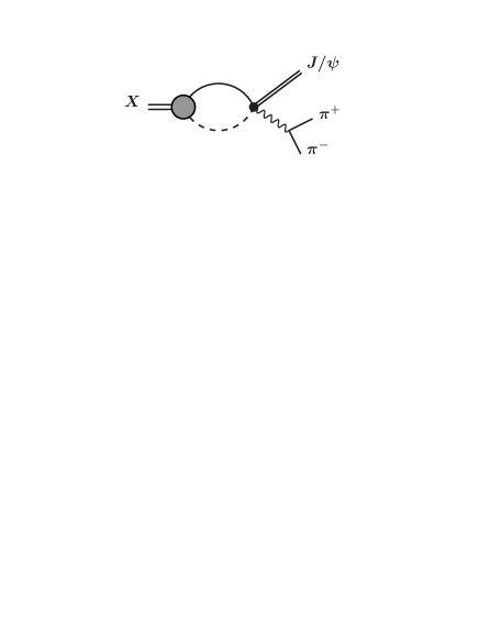
Figure 2: Feynman diagram for $X\to J/\psi\,\pi^{+}\pi^{-}$ that scale like $(am_{\pi})^{-1/2}$. The $(DD^{*})^{0}_{+}$ wavefunction of the $X$ is the integral over the loop energy of the product of the blob and the attached propagators.

The leading terms in the T-matrix element for $X\to H$ in the limit $|a|m_{\pi}\gg 1$ can be represented by the Feynman diagrams in Fig. 2 and can be expressed as

$${\cal T}[X\to H]=\sqrt{2m_{X}}\int{d^{3}p\over(2\pi)^{3}}\,\psi(p)\,{\cal A}^{(\Lambda)}[(DD^{*})^{0}_{+}\to H],$$ (36)

where $\psi(p)$ is the universal wavefunction in Eq. (5). The factor ${\cal A}^{(\Lambda)}$, which is represented by a dot in Fig. 2, is an amplitude for the transition $(DD^{*})^{0}_{+}\to H$ in which all virtual particles are off their energy shells by more than $\Lambda^{2}/(2\mu)$. It is therefore insensitive to the relative momentum $\bm{p}$ of the $D$ and $D^{*}$. If that momentum dependence is neglected and if the integral in Eq. (36) is regularized by a momentum cutoff $|\bm{p}|<\Lambda$, the wavefunction factor reduces in the limit $|a|\gg\Lambda^{-1}$ to

$$\int{d^{3}p\over(2\pi)^{3}}\psi(p)=\sqrt{2\over\pi^{3}}\Lambda a^{-1/2}.$$ (37)

The factorization formula in Eq. (32) is then obtained by absorbing a factor of $(\mu/\pi^{2})\Lambda$ into ${\cal A}^{(\Lambda)}$ to obtain the short-distance factor:

$${\cal A}_{\rm short}[(DD^{*})^{0}_{+}\to H]=\left({\mu\over\pi^{2}}\Lambda\right){\cal A}^{(\Lambda)}[(DD^{*})^{0}_{+}\to H].$$ (38)

Since the T-matrix element in Eq. (32) is independent of the arbitrary separation scale, the dependence on $\Lambda$ must cancel between the two factors on the right side of Eq. (38).

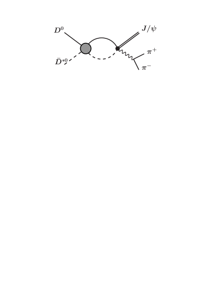
Figure 3: Feynman diagrams for $D^{0}\bar{D}^{*0}\to J/\psi\,\pi^{+}\pi^{-}$ that are enhanced near the $D^{0}\bar{D}^{*0}$ threshold by a factor of $am_{\pi}$. The blob represents the geometric series of Feynman diagrams in Fig. 1.

The leading term in the T-matrix element for $D^{0}\bar{D}^{*0}\to H$ in the limits $|a|\gg\Lambda^{-1}$ and $E\ll\Lambda^{2}/(2\mu)$ can be represented by the Feynman diagram in Fig. 3 and can be expressed as

$${\cal T}[D^{0}\bar{D}^{*0}\to H]={1\over\sqrt{2}}\,\sqrt{4m_{D^{0}}m_{D^{*0}}}\,{\cal A}(E)\,L(\Lambda,E)\,{\cal A}^{(\Lambda)}[(DD^{*})^{0}_{+}\to H].$$ (39)

The factor $L(\Lambda,E)$ is the amplitude for the propagation of the $D$ and $D^{*}$ between successive contact interactions, which is given in Eq. (9). The approximation $E\ll\Lambda^{2}/(2\mu)$ justifies neglecting the $\sqrt{2\mu E}$ term in $L(\Lambda,E)$. The factorization formula in Eq. (34) is then obtained by absorbing the remaining term $(\mu/\pi^{2})\Lambda$ into ${\cal A}^{(\Lambda)}$ to obtain the short-distance factor in Eq. (38).

The factorization formula for the T-matrix element in Eq. (32) implies a factorization formula for the decay rate for $X\to H$. The decay rate $\Gamma[X\to H]$ can be expressed as the product of a short-distance factor and the long-distance factor

$$|{\cal A}_{X}|^{2}={2\pi\over\mu^{2}}\sqrt{\gamma_{\rm re}^{2}+\gamma_{\rm im}^{2}}.$$ (40)

Using the expressions for the binding energy and the total width of the $X$ in Eqs. (14) and (13b), the long-distance factor in Eq. (40) can be expressed as

$$|{\cal A}_{X}|^{2}=\sqrt{8\pi^{2}\over\mu^{3}}[E_{X}+\Gamma_{X}^{2}/(16E_{X})]^{1/2}.$$ (41)

If the partial width for a short-distance decay mode of the $X$ has been calculated using a model with a specific binding energy, the factorization formula for the decay rate can be used to extrapolate the prediction to other values of the binding energy and to take into account the effect of the width of the $X$. This is useful because numerical calculations in models often become increasingly unstable as the binding energy is tuned to zero. Swanson has estimated the partial widths for various short-distance decays of $X$ using a potential model, but only for binding energies down to about 1 MeV and without taking into account the effect of the width of the $X$ Swanson:2003tb ; Swanson:2004pp . His predictions can be extrapolated to other values of the binding energy and the width of the $X$ can be taken into account by using the long-distance factor in Eq. (41).

IV Production of $\bm{X}$

The production of $X$ necessarily involves the long-distance momentum scale $1/|a|$ through the $(DD^{*})^{0}_{+}$ wavefunction of the $X$. The production also involves much larger momentum scales. Unless there are already hadrons in the initial state containing a $c$ and $\bar{c}$, the production process involves the scale $m_{c}$ associated with the creation of a $c\bar{c}$ pair. Even if the initial state includes hadrons that contain $c$ and $\bar{c}$, such as $J/\psi$ or $D^{+}$ and $D^{-}$, the production process involves the scale $m_{\pi}$ associated with the formation of the $D^{0}$ and $\bar{D}^{*0}$ that bind to form the $X$. We will define a short-distance production process to be one for which the initial state either does not include any of the charm mesons $D^{0}$, $\bar{D}^{*0}$, $D^{*0}$, or $\bar{D}^{0}$, or if it does, the momentum of the charm meson in the rest frame of the $X$ is of order $m_{\pi}$ or larger. All practical production mechanisms for $X$ in high energy physics are short-distance processes. Long-distance production mechanisms could arise in a hadronic medium that includes charm mesons, such as that produced by relativistic heavy-ion collisions.

In a short-distance production process, the separation between the long-distance scale $1/|a|$ and all the shorter-distance momentum scales can be exploited through a factorization formula that expresses the leading term in the production rate as the product of a long-distance factor that involves $a$ and a short-distance factor that is insensitive to $a$. To be definite, we will consider the specific production process $B\to XK$. The factorization for any other short-distance production process will have the same long-distance factor but a different short-distance factor.

There are many momentum scales that play an important role in the decay $B\to XK$, ranging from the extremely short-distance scales $m_{W}$ and $m_{b}$ associated with the quark decay process $b\to c\bar{c}s$ to the smaller short-distance scales $\Lambda_{\rm QCD}$ and $m_{\pi}$ involved in formation of the final-state hadrons to the long-distance scale $1/|a|$ associated with the $(DD^{*})^{0}_{+}$ wavefunction of the $X$. We denote the arbitrary boundary between the long-distance momentum region and the short-distance momentum region by $\Lambda$.

The separation between the long-distance scale $1/|a|$ and all the short-distance momentum scales in the decay $B\to XK$ can be exploited through a factorization formula for the T-matrix element:

$${\cal T}[B\to XK]={\cal A}_{\rm short}[B\to(DD^{*})^{0}_{+}K]\times{\cal A}_{X}\sqrt{2m_{X}}.$$ (42)

In the long-distance factor, ${\cal A}_{X}$ is the universal amplitude in Eq. (33). The short-distance factor in Eq. (42) is insensitive to $a$ and one can therefore take the limit $|a|\to\infty$ in that factor. The factorization formula in (42) can serve as the definition of the short-distance factor. The content of the factorization statement then resides in the fact that the same short-distance factor appears in the factorization formula for the T-matrix element for the decay $B\to D^{0}\bar{D}^{*0}K$ when the $DD^{*}$ invariant mass is near the $D^{0}\bar{D}^{*0}$ threshold. This factorization formula is discussed in Section V.

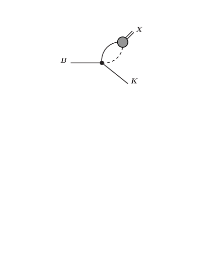
Figure 4: Feynman diagram for $B\to XK$ that scales like $(am_{\pi})^{-1/2}$. The $(DD^{*})^{0}_{+}$ wavefunction of the $X$ is the integral over the loop energy of the product of the blob and the attached propagators.

The factorization formula in Eq. (42) can be motivated diagrammatically by separating the loop integrals in the decay amplitude according to whether the virtual particles are off their energy shells by less than or by more than $\Lambda^{2}/(2\mu)$. The leading terms in the decay amplitude for $B\to XK$ are suppressed only by a factor of $(am_{\pi})^{-1/2}$. These terms can be represented by the Feynman diagram in Fig. 4 and can be expressed in the form

$${\cal T}[B\to XK]=\sqrt{2m_{X}}\int{d^{3}p\over(2\pi)^{3}}\psi(p)\,{\cal A}^{(\Lambda)}[B\to(DD^{*})^{0}_{+}K],$$ (43)

where $\psi(p)$ is the universal wavefunction in Eq. (5). The factor ${\cal A}^{(\Lambda)}$, which is represented by a dot in Fig. 4, is an amplitude for the decay $B\to(DD^{*})^{0}_{+}K$ in which all virtual particles are off their energy shells by more than $\Lambda^{2}/(2\mu)$. It is therefore insensitive to the relative momentum $\bm{p}$ of the $D$ and $D^{*}$. If that momentum dependence is neglected, the wavefunction factor in Eq. (43) reduces to Eq. (37). The factorization formula in Eq. (42) then requires the short-distance factor to be

$${\cal A}_{\rm short}[B\to(DD^{*})^{0}_{+}K]={\cal A}^{(\Lambda)}[B\to(DD^{*})^{0}_{+}K]\left({\mu\over\pi^{2}}\Lambda\right).$$ (44)

Since the T-matrix element in Eq. (42) is independent of the arbitrary separation scale, the dependence on $\Lambda$ must cancel between the two factors on the right side of Eq. (44).

We proceed to use the factored expression in Eq. (42) to evaluate the decay rate for $B^{+}\to XK^{+}$. Lorentz invariance constrains the short-distance amplitude ${\cal A}_{\rm short}$ at the $DD^{*}$ threshold to have the form

$${\cal A}_{\rm short}[B^{+}\to(DD^{*})^{0}_{+}K^{+}]=c_{+}\,P\cdot\epsilon_{D^{*}},$$ (45)

where $P$ is the 4-momentum of the $B^{+}$ and $\epsilon_{D^{*}}$ is the polarization 4-vector of the $D^{*}$. Heavy quark spin symmetry guarantees that the polarization vector $\epsilon_{D^{*}}$ can be identified with the polarization vector $\epsilon_{X}$ of the $X$. The decay rate is obtained by squaring the amplitude in Eq. (42), summing over the spin of the $X$, and integrating over phase space. The resulting expression for the decay rate is

$$\Gamma[B^{+}\to XK^{+}]=|c_{+}|^{2}{\lambda^{3/2}(m_{B},m_{X},m_{K})\over 32\pi m_{B}^{3}m_{X}}\big{|}{\cal A}_{X}|^{2},$$ (46)

where $\lambda(x,y,z)$ is the triangle function:

$$\lambda(x,y,z)=x^{4}+y^{4}+z^{4}-2(x^{2}y^{2}+y^{2}z^{2}+z^{2}x^{2}).$$ (47)

The long-distance factor $|{\cal A}_{X}|^{2}$ is given in Eq. (40). The result in Eq. (46) was obtained in Ref. Braaten:2004fk for the special case $\gamma_{\rm im}=0$ and used to estimate the order of magnitude of the decay rate for $B^{+}\to XK^{+}$. The estimate is consistent with the measurement of the product of the branching fractions for $B^{+}\to XK^{+}$ and $X\to J/\psi\,\pi^{+}\pi^{-}$ Choi:2003ue provided $J/\psi\pi^{+}\,\pi^{-}$ is one of the major decay modes of $X$.

The factorization formula for the decay rate for $B^{0}\to XK^{0}$ has the same form as in Eq. (46) except that the coefficient $c_{+}$ in the short-distance decay amplitude in Eq. (45) has a different value. In Ref. Braaten:2004ai , it was pointed out that the decay rate for $B^{0}\to XK^{0}$ should be suppressed compared to $B^{+}\to XK^{+}$. That suppression can be understood by considering the short-distance amplitude for $B\to DD^{*}K$. The dominant contributions to most decay amplitudes of the $B$ meson are believed to be factorizable into the product of matrix elements of currents. The factorizable contributions to the decay amplitude for $B^{+}\to(DD^{*})^{0}_{+}K^{+}$ have three terms: the product of $B^{+}\to\bar{D}^{*0}$ and $\emptyset\to D^{0}K^{+}$ matrix elements, where $\emptyset$ is the QCD vacuum, the product of $B^{+}\to\bar{D}^{0}$ and $\emptyset\to D^{*0}K^{+}$ matrix elements, and the product of $B^{+}\to K^{+}$ and $\emptyset\to(DD^{*})^{0}_{+}$ matrix elements. The factorizable contributions to the decay amplitude for $B^{0}\to(DD^{*})^{0}_{+}K^{0}$ have only one term: the product of $B^{0}\to K^{0}$ and $\emptyset\to(DD^{*})^{0}_{+}$ matrix elements. Heavy quark symmetry implies that the $\emptyset\to(DD^{*})^{0}_{+}$ matrix element vanishes at the $D^{0}\bar{D}^{*0}$ threshold. The decay $B^{0}\to(DD^{*})^{0}_{+}K^{0}$ near the $D^{0}\bar{D}^{*0}$ threshold must therefore proceed through nonfactorizable terms in the decay amplitude. The resulting suppression of the coefficient $c_{+}$ in the short-distance factor for $B^{0}\to(DD^{*})^{0}_{+}K^{0}$ results in a suppression of the rate for $B^{0}\to XK^{0}$ relative to the rate for $B^{+}\to XK^{+}$. In Ref. Braaten:2004ai , a quantitative analysis of Babar data on the branching fractions for $B\to D^{(*)}D^{(*)}K$ Aubert:2003jq was used to estimate the suppression factor to be an order of magnitude or more.

V Production of $\bm{D^{0}{\bar{D}^{*0}}}$ Near Threshold

It was pointed out in Ref. Braaten:2004fk that the identification of $X$ as a $DD^{*}$ molecule could be confirmed by observing a peak in the invariant mass distribution for $D^{0}\bar{D}^{*0}$ (or $D^{*0}\bar{D}^{0}$) near the $DD^{*}$ threshold in the decay $B\to DD^{*}K$. The shape of that invariant mass distribution was given for a real scattering length $a$. The shape would be the same for any other short-distance production process. In this section, we consider the effect of an imaginary part of the scattering length on the $DD^{*}$ invariant mass distribution for a short-distance production process. To be specific, we consider the short-distance production process $B\to D^{0}\bar{D}^{*0}K$.

The separation between the long-distance scale $1/|a|$ and all the short-distance momentum scales in the decay $B\to D^{0}\bar{D}^{*0}K$ can be exploited through a factorization formula for the T-matrix element:

$${\cal T}[B\to D^{0}\bar{D}^{*0}K]={\cal A}_{\rm short}[B\to(DD^{*})^{0}_{+}K]\times{\cal A}(E)\,\sqrt{4m_{D^{0}}m_{D^{*0}}}\,{1\over\sqrt{2}}.$$ (48)

In the long-distance factor, ${\cal A}(E)$ is the universal amplitude in Eq. (35) and the factor $1/\sqrt{2}$ is the amplitude for $D^{0}\bar{D}^{*0}$ to be in the channel $(DD^{*})^{0}_{+}$ with the large scattering length. The short-distance factor ${\cal A}_{\rm short}$ is the same as in the factorization formula for $B\to XK$ in Eq. (42).

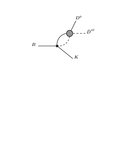
Figure 5: Feynman diagrams for $B\to D^{0}\bar{D}^{*0}K$ that are enhanced near the $D^{0}\bar{D}^{*0}$ threshold by a factor of $am_{\pi}$. The blob represents the geometric series of diagrams shown in Fig. 1.

The factorization formula in Eq. (48) can be motivated diagrammatically by separating the loop integrals in the decay amplitude according to whether the virtual particles are off their energy shells by less than or by more than $\Lambda^{2}/(2\mu)$. There are terms in the T-matrix element for the decay $B\to D^{0}\bar{D}^{*0}K$ that are enhanced near the $DD^{*}$ threshold by a factor of $am_{\pi}$. These terms can be represented by the Feynman diagrams in Fig. 5 and can be expressed in the form

$${\cal T}[B\to D^{0}\bar{D}^{*0}K]={\cal A}^{(\Lambda)}[B\to(DD^{*})^{0}_{+}K]\,L(\Lambda,E)\,{\cal A}(E)\,\sqrt{4m_{D^{0}}m_{D^{*0}}}\,{1\over\sqrt{2}}.$$ (49)

The first factor ${\cal A}^{(\Lambda)}$, which is represented by the dot in Fig. 5, is an amplitude for the decay into $(DD^{*})^{0}_{+}K$ in which all virtual particles are off their energy shells by more than $\Lambda^{2}/(2\mu)$. It is therefore insensitive to the relative momentum $\bm{p}$. The second factor $L(\Lambda,E)$ is the amplitude for the propagation of the $D$ and $D^{*}$ between contact interactions, which is given in Eq. (9). The condition $|E|\ll\Lambda^{2}/(2\mu)$ implies that the $\sqrt{-2\mu E}$ term in $L(\Lambda,E)$ can be neglected. The resulting expression for the T-matrix element is the factorization formula in Eq. (48), with the short-distance factor ${\cal A}_{\rm short}$ given in Eq. (44).

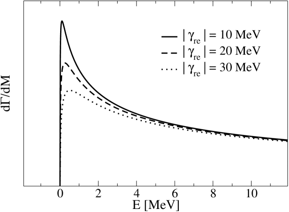
Figure 6: The $DD^{*}$ invariant mass distribution in $B\to D^{0}\bar{D}^{*0}K$ for $\gamma_{\rm im}=10$ MeV and various values of $|\gamma_{\rm re}|/\gamma_{\rm im}$. The horizontal axis is the difference $E=M-(m_{D^{0}}+m_{D^{*0}})$ between the invariant mass $M$ and the $D^{0}\bar{D}^{*0}$ threshold.

We proceed to use the factorized expression for the decay amplitude in Eq. (48) to calculate the $DD^{*}$ invariant mass distribution near the $D^{0}\bar{D}^{*0}$ threshold in the decay $B^{+}\to D^{0}\bar{D}^{*0}K^{+}$. Lorentz invariance constrains the short-distance amplitude ${\cal A}_{\rm short}$ at the $DD^{*}$ threshold to have the form in Eq. (45). The decay rate is obtained by squaring the amplitude in Eq. (48), summing over the spins of the $\bar{D}^{*0}$, and integrating over phase space. The resulting expression for the differential decay rate with respect to the $DD^{*}$ invariant mass $M$ near the $D^{0}\bar{D}^{*0}$ threshold is

$${d\Gamma\over dM}[B^{+}\to D^{0}\bar{D}^{*0}K^{+}]=|c_{+}|^{2}{\mu\,\lambda^{3/2}(m_{B},M,m_{K})\over 256\pi^{3}m_{B}^{3}M^{2}}\,\lambda^{1/2}(M,m_{D^{0}},m_{D^{*0}})\,|{\cal A}(E)|^{2},$$ (50)

where $E$ is the energy of the $D^{0}\bar{D}^{*0}$ in its rest frame relative to the $D^{0}\bar{D}^{*0}$ threshold:

$$E=M-(m_{D^{0}}+m_{D^{*0}}).$$ (51)

We have used the fact that $M$ is near the $D^{0}\bar{D}^{*0}$ threshold to replace a factor of $m_{D^{0}}m_{D^{*0}}$ in Eq. (50) by $\mu M$. The result in Eq. (50) was obtained previously in Ref. Braaten:2004fk for the special case $\gamma_{\rm im}=0$. For $M$ near the $D^{0}\bar{D}^{*0}$ threshold, the only significant variation with $M$ is through the long-distance factor $|{\cal A}(E)|^{2}$ and the threshold factor

$$\lambda^{1/2}(M,m_{D^{0}},m_{D^{*0}})\approx 2M\sqrt{2\mu E}.$$ (52)

If the complex scattering length is parameterized as in Eq. (12), the long-distance factor is

$$|{\cal A}(E)|^{2}={4\pi^{2}/\mu^{2}\over((2\mu E)^{1/2}+\gamma_{\rm im})^{2}+\gamma_{\rm re}^{2}}.$$ (53)

The shape of the $D^{0}\bar{D}^{*0}$ invariant mass distribution in Eq. (50) is given by the factor $\sqrt{2\mu E}\,|{\cal A}(E)|^{2}$. Note that it depends on $\gamma_{\rm re}$ and $\gamma_{\rm im}$ but not on the sign of $\gamma_{\rm re}$. The invariant mass distribution is shown in Fig. 6 for $\gamma_{\rm im}=10$ MeV and three values of $|\gamma_{\rm re}|$: 10, 20, and 30 MeV. The peak in the invariant mass distribution occurs at $E=|\gamma|^{2}/(2\mu)$, where $|\gamma|=\sqrt{\gamma_{\rm re}^{2}+\gamma_{\rm im}^{2}}$. The value at the peak is proportional to $(|\gamma|+\gamma_{\rm im})^{-1}$. The full width at half maximum is $2(2|\gamma|+\gamma_{\rm im})[(|\gamma|+\gamma_{\rm im})(3|\gamma|+\gamma_{\rm im})]^{1/2}/\mu$.

VI The $\bm{X}$ Line Shape

The $X$ is observed as a peak in the invariant mass distribution of its decay products, such as $J/\psi\,\pi^{+}\pi^{-}$. Its mass and width are extracted from that invariant mass distribution. For instance, the Belle collaboration obtained their value for the mass and the upper bound on the width by fitting the $J/\psi\,\pi^{+}\pi^{-}$ invariant mass distribution in $B^{+}\to J/\psi\,\pi^{+}\pi^{-}\,K^{+}$ near the $D^{0}\bar{D}^{*0}$ threshold to a resolution-broadened Breit-Wigner function on top of a polynomial background. The shape of the invariant mass distribution of the decay products of the $X$ is called the line shape. The resonant interactions in the $D^{0}\bar{D}^{*0}/D^{*0}\bar{D}^{0}$ system can significantly modify the line shape, so it need not have the conventional Breit-Wigner form. In this section, we compute the line shape of the $X$ in short-distance decays of the $X$. To be definite, we consider the production process $B\to HK$, where $H$ is the hadronic system consisting of $J/\psi\,\pi^{+}\pi^{-}$ with invariant mass near the $D^{0}\bar{D}^{*0}$ threshold. However our results on the line shape will apply more generally to any short-distance production process for $X$ and any short-distance decay mode of $X$.

The separation between the long-distance scale $1/|a|$ and all the short-distance momentum scales in the decay $B\to HK$ can be exploited through a factorization formula for the T-matrix element:

$${\cal T}[B\to HK]={\cal A}_{\rm short}[B\to(DD^{*})^{0}_{+}K]\times{\cal A}(E)\times{\cal A}_{\rm short}[(DD^{*})^{0}_{+}\to H].$$ (54)

There is an implied sum over the spin states of the $D^{*}$. The long-distance factor ${\cal A}(E)$ depends on the complex-valued scattering length $a$ and is given in Eq. (35). Its argument $E$ is the difference between the invariant mass $M$ of the hadronic system $H$ and the $D^{0}\bar{D}^{*0}$ threshold, as given in Eq. (51). The short-distance factor ${\cal A}_{\rm short}$ associated with the initial state is the same one that appears in the factorization formulas for $B\to XK$ in Eq. (42) and for $B\to D^{0}\bar{D}^{*0}K$ in Eq. (48). The short-distance factor ${\cal A}_{\rm short}$ associated with the final state is the same one that appears in the factorization formulas for $X\to H$ in Eq. (32) and for $D^{0}\bar{D}^{*0}\to H$ in Eq. (34).

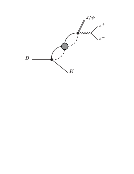
Figure 7: Feynman diagrams for $B\to J/\psi\,\pi^{+}\pi^{-}\,K$ that are enhanced near the $D^{0}\bar{D}^{*0}$ threshold by a factor of $am_{\pi}$. The blob represents the geometric series of diagrams given in Fig. 1.

The factorization formula in Eq. (54) can be motivated diagrammatically by separating the loop integrals in the decay amplitude according to whether the virtual particles are off their energy shells by less than or by more than $\Lambda^{2}/(2\mu)$. There are terms in the decay amplitude for $B\to HK$ that are enhanced by a factor of $am_{\pi}$ when the invariant mass of $H$ is near the $D^{0}\bar{D}^{*0}$ threshold. These terms can be represented by the Feynman diagrams in Fig. 7 and can be expressed in the form

$${\cal T}[B\to HK] = {\cal A}^{(\Lambda)}[B\to(DD^{*})^{0}_{+}K]\,L(\Lambda,E)\,{\cal A}(E)\,L(\Lambda,E)\,{\cal A}^{(\Lambda)}[(DD^{*})^{0}_{+}\to H].$$ (55)

The factors ${\cal A}^{(\Lambda)}$, which are represented by dots in Fig. 7, are amplitudes in which all virtual particles are off their energy shells by more than $\Lambda^{2}/(2\mu)$. The factors of $L(\Lambda,E)$, which is given in Eq. (9), are the amplitudes for the propagation of the $D$ and $D^{*}$ between contact interactions. The condition $|E|\ll\Lambda^{2}/(2\mu)$ implies that the $\sqrt{-2\mu E}$ term in $L(\Lambda,E)$ can be neglected. The resulting expression for the T-matrix element is the factorization formula in Eq. (54), with the short-distance factors ${\cal A}_{\rm short}$ given in Eqs. (44) and (38).

The factorization formula for the T-matrix element in (54) implies a factorization formula for the invariant mass distribution for the hadronic system $H$ near the $D^{0}\bar{D}^{*0}$ threshold. If the hadronic system consists of particles with momenta $p_{i}$ and invariant mass $M$, the factorization formula is

$$\frac{d\Gamma}{dM}[B^{+}\to K^{+}H]$$ (56)

$$= {M\over 2\pi m_{B}}\int\big{|}{\cal A}_{\rm short}[B\to(DD^{*})^{0}_{+}K]\big{|}^{2}(2\pi)^{4}\delta^{4}(P_{B}-P_{H}-P_{K}){d^{3}P_{H}\over(2\pi)^{3}2E_{H}}{d^{3}P_{K}\over(2\pi)^{3}2E_{K}}$$

$$\times|{\cal A}(E)|^{2}\times\int\big{|}{\cal A}_{\rm short}[(DD^{*})^{0}_{+}\to H]\big{|}^{2}(2\pi)^{4}\delta^{4}(P_{H}-\mbox{$\sum$}_{i}p_{i})\prod_{i}{d^{3}p_{i}\over(2\pi)^{3}2E_{i}}.$$

For $M$ near the $D^{0}\bar{D}^{*0}$ threshold, the only significant variation with $M$ is through the long-distance factor $|{\cal A}(E)|^{2}$, where $E$ is the energy defined in Eq. (51). If the complex scattering length is parameterized as in Eq. (12), the long-distance factor is

$$\bigl{|}{\cal A}(E)\bigr{|}^{2} = \frac{4\pi^{2}/\mu^{2}}{(|2\mu E|^{1/2}-\gamma_{\rm re})^{2}+\gamma_{\rm im}^{2}}\hskip 59.75095pt\;E\leq 0,$$ (57a)

$$= \frac{4\pi^{2}/\mu^{2}}{((2\mu E)^{1/2}+\gamma_{\rm im})^{2}+\gamma_{\rm re}^{2}}\hskip 56.9055pt\;E\geq 0.$$ (57b)

This factor gives the line shape of the $X$. Note that for $E>0$, the line shape does not depend on the sign of $\gamma_{\rm re}$. However for $E<0$, the line shape is completely different for $\gamma_{\rm re}>0$ and $\gamma_{\rm re}<0$.

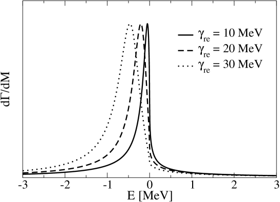
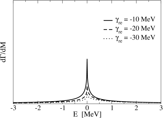
Figure 8: The $X$ line shape in a short-distance decay channel, such as $J/\psi\,\pi^{+}\pi^{-}$, for $\gamma_{\rm im}=10$ MeV and for various positive values (upper panel) and various negative values (lower panel) of $\gamma_{\rm re}/\gamma_{\rm im}$. The horizontal axis is the difference $E=M-(m_{D^{0}}+m_{D^{*0}})$ between the invariant mass $M$ and the $D^{0}\bar{D}^{*0}$ threshold.

In the case $\gamma_{\rm re}>0$, the peak in the invariant mass distribution occurs below the $D^{0}\bar{D}^{*0}$ threshold by the amount $\gamma_{\rm re}^{2}/(2\mu)$. The $X$ line shape is illustrated in the upper panel of Fig. 8 for $\gamma_{\rm im}=10$ MeV and for three positive values of $\gamma_{\rm re}$: 10, 20, and 30 MeV. If $\gamma_{\rm im}<\gamma_{\rm re}$, the full width of the peak at half maximum is $2\gamma_{\rm re}\gamma_{\rm im}/\mu$. The line shape for $E<0$ is symmetric about the peak as a function of $|E|^{1/2}$ but not as a function of $E$. If $\gamma_{\rm im}\ll\gamma_{\rm re}$, the line shape in Eq. (57) is sharply peaked at $E=-\gamma_{\rm re}^{2}/(2\mu)$ and it can be approximated by a delta function:

$$|{\cal A}(E)|^{2}\approx{4\pi^{3}\gamma_{\rm re}\over\mu^{3}\gamma_{\rm im}}\delta\big{(}E+\gamma_{\rm re}^{2}/(2\mu)\big{)}.$$ (58)

Note that the condition $\gamma_{\rm im}\ll\gamma_{\rm re}$ is equivalent to $\Gamma_{X}\ll E_{X}/4$.

In the case $\gamma_{\rm re}<0$, the peak in the invariant mass distribution occurs at the $D^{0}\bar{D}^{*0}$ threshold. The $X$ line shape is illustrated in the lower panel of Fig. 8 for $\gamma_{\rm im}=10$ MeV and for three negative values of $\gamma_{\rm re}$: $-10$, $-20$, and $-30$ MeV. The line shape has a cusp at $E=0$. Bugg has proposed that the $X$ can be identified with this cusp at the $D^{0}\bar{D}^{*0}$ threshold Bugg:2004rk . The normalization is the same in the upper and lower panels of Fig. 8. Note that the area under the cusp in the lower panel of Fig. 8 is much smaller than the area under the resonance in the upper panel for the same values of $\gamma_{\rm im}$ and $|\gamma_{\rm re}|$. Thus a cusp seems less likely as an interpretation for the $X(3872)$ than a resonance, although a quantitative analysis would be required to rule out that possibility.

The integral over all energies of the line shape of a conventional Breit-Wigner resonance is convergent. In contrast, the integral of the line shape in Eq. (57) diverges logarithmically as the endpoints $E_{\rm min}$ and $E_{\rm max}$ of the integral increase in magnitude. This follows from the fact that the line shape in Eq. (57) decreases as $1/|E|$ for $(2\mu|E|)^{1/2}\gg|\gamma_{\rm re}|,\gamma_{\rm im}$. That expression for the line shape is of course only accurate for $|E|$ lower than $\Lambda^{2}/(2\mu)\sim 10$ MeV, where $\Lambda\sim m_{\pi}$ is the natural momentum scale for low-energy $DD^{*}$ scattering. Thus the logarithmic dependence on $E_{\rm min}$ and $E_{\rm max}$ holds only for $|E_{\rm min}|,E_{\rm max}<\Lambda^{2}/(2\mu)$. It is convenient to define $p_{\rm min}$ and $p_{\rm max}$ by $E_{\rm min}=-p_{\rm min}^{2}/(2\mu)$ and $E_{\rm max}=+p_{\rm max}^{2}/(2\mu)$. The integral of the factor in Eq. (57) reduces in the limit $p_{\rm min},p_{\rm max}\gg|\gamma_{\rm re}|,\gamma_{\rm im}$ to

$$\int_{E_{\rm min}}^{E_{\rm max}}|{\cal A}(E)|^{2}dE\approx{4\pi^{2}\over\mu^{3}}\left(\log{p_{\rm min}p_{\rm max}\over\gamma_{\rm re}^{2}+\gamma_{\rm im}^{2}}+{\pi\gamma_{\rm re}\over\gamma_{\rm im}}\,\theta(\gamma_{\rm re})-f(\gamma_{\rm re}/\gamma_{\rm im})\right),$$ (59)

where $f(x)$ is the function

$$f(x)=x\arctan(1/x)+(1/x)\arctan(x).$$ (60)

This function has a limited range, varying from 1 at $x=0$ and $x=\pm\infty$ to $\pi/2$ at $x=\pm 1$.

The factorization formula for the invariant mass distribution of $H$ in the case $\gamma_{\rm re}>0$ has important implications for measurements of the branching fractions of $X$. Since the two short-distance factors in Eq. (56) are insensitive to $E$, we can set $M$ to $m_{D^{0}}+m_{D^{*0}}$ or to $m_{X}$ in those factors. The short-distance factor associated with the decay of the $B^{+}$ reduces to $\Gamma[B\to XK]/(2\pi|{\cal A}_{X}|^{2})$. If $\gamma_{\rm re}>0$, the short-distance factor associated with the formation of $H$ reduces to $\Gamma[X\to H]/|{\cal A}_{X}|^{2}$. Thus the differential decay rate in Eq. (56) reduces to

$${d\Gamma\over dM}[B\to HK]=\Gamma[B\to XK]\,{\rm Br}[X\to H]\;{\Gamma_{X}\,|{\cal A}(E)|^{2}\over 2\pi\,|{\cal A}_{X}|^{4}}.$$ (61)

If the product of $\Gamma[B\to XK]$ and ${\rm Br}[X\to H]$ is measured by integrating $d\Gamma/dM$ over the energy interval from $E_{\rm min}$ to $E_{\rm max}$ with $|E_{\rm min}|,E_{\rm max}\gg E_{X},\Gamma_{X}$, it will be in error by the factor

$${\Gamma_{X}\over 2\pi|{\cal A}_{X}|^{4}}\int_{E_{\rm min}}^{E_{\rm max}}|{\cal A}(E)|^{2}dE \approx \left[1+{\Gamma_{X}^{2}\over 16E_{X}^{2}}\right]^{-1}$$ (62)

$$\times\left[1+\left(\log{|E_{\rm min}|^{1/2}E_{\rm max}^{1/2}\over E_{X}+\Gamma_{X}^{2}/(16E_{X})}-f(4E_{X}/\Gamma_{X})\right){\Gamma_{X}\over 4\pi E_{X}}\right].$$

The error would cancel in the ratio of the branching fractions for any two short-distance decay modes of $X$. The error would not cancel in the ratio of the branching fractions for a short-distance decay mode of $X$ and one of the long-distance decay modes $D^{0}\bar{D}^{0}\pi^{0}$ and $D^{0}\bar{D}^{0}\gamma$. This effect should be taken into account in analyzing the decays of the $X(3872)$.

VII Summary

If the $X(3872)$ is a loosely-bound S-wave molecule corresponding to a $C=+$ superposition of $D^{0}\bar{D}^{*0}$ and $D^{*0}\bar{D}^{0}$, the scattering length $a$ in the $(DD^{*})_{+}^{0}$ channel is large compared to all other length scales of QCD. The decays of the $X$ implies that the large scattering length has an imaginary part. It can be conveniently parameterized in terms of the real and imaginary parts of $1/a$ as in Eq. (12). The binding energy $E_{X}$ and the width $\Gamma_{X}$ are expressed in terms of those parameters in Eqs. (14) and (13b).

The large scattering length can be exploited through factorization formulas for decay rates of $X$. For short-distance decay modes that do not proceed through the decay of a constituent $D^{*}$ of the $X$, the long-distance factor in the factorization formula is proportional to $1/|a|$ and is given in Eq. (41). If a partial width of the $X$ is calculated using some model with a specific binding energy for the $X$, the factorization formulas can be used to extrapolate the prediction to other values of the binding energy and to take into account the width of the $X$.

The large scattering length can also be exploited through factorization formulas for production rates of $X$, $D^{0}\bar{D}^{*0}$ near threshold, $D^{*0}\bar{D}^{0}$ near threshold, and decay products of $X$ with invariant mass near the $D^{0}\bar{D}^{*0}$ threshold. The long-distance factor in the factorization formula for production rates of $X$ is proportional to $1/|a|$. For production of $D^{0}\bar{D}^{*0}$ and $D^{*0}\bar{D}^{0}$ near threshold, the factorization formula implies that the dependence on the invariant mass is through the factor $\sqrt{2\mu E}|{\cal A}(E)|^{2}$, where $E$ is the invariant mass relative to the $D^{0}\bar{D}^{*0}$ threshold and $|{\cal A}(E)|^{2}$ is given in Eq. (53). The peak in the invariant mass distribution is above the threshold by the amount $E_{X}+\Gamma_{X}^{2}/(16E_{X})$. The line shape of the $X$ can be measured through the invariant mass distribution of its decay products. In the case of short-distance decay modes, the factorization formulas imply that near the $D^{0}\bar{D}^{*0}$ threshold, the shape of the invariant mass distribution is given by the factor $|{\cal A}(E)|^{2}$ in Eq. (57). If Re$(a)<0$, the distribution has a cusp at $E=0$, as shown in the lower panel of Fig. 8. If Re$(a)>0$, the distribution has a peak at $E=-E_{X}$, as shown in the upper panel of Fig. 8. In contrast to a Breit-Wigner resonance, the integral over the line shape is logarithmically sensitive to the endpoints of the integration region. This effect should be taken into account in analyzing the production and decay of the $X$.

- (1) S. K. Choi et al. [Belle Collaboration], Phys. Rev. Lett. 91, 262001 (2003). [arXiv:hep-ex/0309032].
- (2) B. Aubert et al. [BABAR Collaboration], Phys. Rev. D 71, 071103 (2005) [arXiv:hep-ex/0406022].
- (3) D. Acosta et al. [CDF II Collaboration], Phys. Rev. Lett. 93, 072001 (2004). [arXiv:hep-ex/0312021].
- (4) V. M. Abazov et al. [D0 Collaboration], Phys. Rev. Lett. 93, 162002 (2004) [arXiv:hep-ex/0405004].
- (5) S. L. Olsen [Belle Collaboration], Int. J. Mod. Phys. A 20, 240 (2005) [arXiv:hep-ex/0407033].
- (6) K. Abe, arXiv:hep-ex/0505037.
- (7) K. Abe et al. [Belle Collaboration], Phys. Rev. Lett. 93, 051803 (2004). [arXiv:hep-ex/0307061].
- (8) C. Z. Yuan, X. H. Mo and P. Wang, Phys. Lett. B 579, 74 (2004). [arXiv:hep-ph/0310261].
- (9) B. Aubert et al. [BABAR Collaboration], Phys. Rev. Lett. 93, 041801 (2004). [arXiv:hep-ex/0402025].
- (10) Z. Metreveli et al. [CLEO Collaboration], arXiv:hep-ex/0408057.
- (11) K. Abe et al. [Belle Collaboration], arXiv:hep-ex/0408116.
- (12) T. Barnes and S. Godfrey, Phys. Rev. D 69, 054008 (2004). [arXiv:hep-ph/0311162].
- (13) E. J. Eichten, K. Lane and C. Quigg, Phys. Rev. D 69, 094019 (2004). [arXiv:hep-ph/0401210].
- (14) C. Quigg, arXiv:hep-ph/0403187.
- (15) N.A. Tornqvist, arXiv:hep-ph/0308277.
- (16) N. A. Tornqvist, Phys. Lett. B 590, 209 (2004). [arXiv:hep-ph/0402237].
- (17) M. B. Voloshin, Phys. Lett. B 579, 316 (2004). [arXiv:hep-ph/0309307].
- (18) C. Y. Wong, Phys. Rev. C 69, 055202 (2004). [arXiv:hep-ph/0311088].
- (19) E. Braaten and M. Kusunoki, Phys. Rev. D 69, 074005 (2004). [arXiv:hep-ph/0311147].
- (20) E. S. Swanson, Phys. Lett. B 588, 189 (2004). [arXiv:hep-ph/0311229].
- (21) E. S. Swanson, Phys. Lett. B 598, 197 (2004) [arXiv:hep-ph/0406080].
- (22) D. V. Bugg, Phys. Lett. B 598, 8 (2004). [arXiv:hep-ph/0406293].
- (23) D. V. Bugg, Phys. Rev. D 71, 016006 (2005) [arXiv:hep-ph/0410168].
- (24) J. Vijande, F. Fernandez and A. Valcarce, Int. J. Mod. Phys. A 20, 702 (2005) [arXiv:hep-ph/0407136].
- (25) F. E. Close and S. Godfrey, Phys. Lett. B 574, 210 (2003) [arXiv:hep-ph/0305285].
- (26) B. A. Li, Phys. Lett. B 605, 306 (2005) [arXiv:hep-ph/0410264].
- (27) K. K. Seth, Phys. Lett. B 612, 1 (2005) [arXiv:hep-ph/0411122].
- (28) L. Maiani, F. Piccinini, A. D. Polosa and V. Riquer, Phys. Rev. D 71, 014028 (2005) [arXiv:hep-ph/0412098].
- (29) F. E. Close and P. R. Page, Phys. Lett. B 578, 119 (2004). [arXiv:hep-ph/0309253].
- (30) S. Pakvasa and M. Suzuki, Phys. Lett. B 579, 67 (2004). [arXiv:hep-ph/0309294].
- (31) J. L. Rosner, Phys. Rev. D 70, 094023 (2004) [arXiv:hep-ph/0408334].
- (32) T. Kim and P. Ko, Phys. Rev. D 71, 034025 (2005) [arXiv:hep-ph/0405265].
- (33) K. Abe, arXiv:hep-ex/0505038.
- (34) C. Quigg, Nucl. Phys. Proc. Suppl. 142, 87 (2005) [arXiv:hep-ph/0407124].
- (35) M. Bander, G. L. Shaw, P. Thomas and S. Meshkov, Phys. Rev. Lett. 36, 695 (1976).
- (36) M. B. Voloshin and L. B. Okun, JETP Lett. 23, 333 (1976).
- (37) A. De Rujula, H. Georgi and S. L. Glashow, Phys. Rev. Lett. 38, 317 (1977).
- (38) S. Nussinov and D. P. Sidhu, Nuovo Cim. A 44, 230 (1978).
- (39) N. A. Tornqvist, Z. Phys. C 61, 525 (1994). [arXiv:hep-ph/9310247].
- (40) E. Braaten and M. Kusunoki, Phys. Rev. D 69, 114012 (2004) [arXiv:hep-ph/0402177].
- (41) E. Braaten, M. Kusunoki and S. Nussinov, Phys. Rev. Lett. 93, 162001 (2004). [arXiv:hep-ph/0404161].
- (42) E. Braaten and M. Kusunoki, Phys. Rev. D 71, 074005 (2005) [arXiv:hep-ph/0412268].
- (43) E. Braaten, arXiv:hep-ph/0408230.
- (44) M. B. Voloshin, Phys. Lett. B 604, 69 (2004) [arXiv:hep-ph/0408321].
- (45) E. Braaten and H. W. Hammer, arXiv:cond-mat/0410417.
- (46) T. D. Cohen, B. A. Gelman and U. van Kolck, Phys. Lett. B 588, 57 (2004). [arXiv:nucl-th/0402054].
- (47) M. J. Savage, Phys. Rev. C 55, 2185 (1997) [arXiv:nucl-th/9611022].
- (48) B. Aubert et al. [Babar Collaboration], Phys. Rev. D 68, 092001 (2003). [arXiv:hep-ex/0305003].