The Meaning of Higgs:
$\tau^{+}\tau^{-}$ and $\gamma\gamma$
at the Tevatron and the LHC

In this paper we discuss how to extract information about physics beyond the Standard Model (SM) from searches for a light SM Higgs at Tevatron Run II and CERN LHC. We demonstrate that new (pseudo)scalar states predicted in both supersymmetric and dynamical models can have enhanced visibility in standard Higgs search channels, making them potentially discoverable at Tevatron Run II and CERN LHC. We discuss the likely sizes of the enhancements in the various search channels for each model and identify the model features having the largest influence on the degree of enhancement. We compare the key signals for the non-standard scalars across models and also with expectations in the SM, to show how one could start to identify which state has actually been found. In particular, we suggest the likely mass reach of the Higgs search in $p\bar{p}/pp\to{\cal H}\to\tau^{+}\tau^{-}$ for each kind of non-standard scalar state and we demonstrate that $p\bar{p}/pp\to{\cal H}\to\gamma\gamma$ may cleanly distinguish the scalars of supersymmetric models from those of dynamical models.

1 Introduction

The origin of electroweak symmetry breaking remains unknown. While the Standard Model (SM) of particle physics is consistent with existing data, theoretical considerations suggest that this theory is only a low-energy effective theory and must be supplanted by a more complete description of the underlying physics at energies above those reached so far by experiment.

The CDF and DØ experiments at the Fermilab Tevatron are currently searching for the Higgs boson of the Standard Model. The production cross-section and decay branching fractions for this state have been predicted in great detail for the mass range accessible to Tevatron Run II. Search strategies have been carefully planned and optimized.

However, if the Tevatron does find evidence for a new scalar state, it may not necessarily be the Standard Higgs. Many alternative models of electroweak symmetry breaking have spectra that include new scalar or pseudoscalar states whose masses could easily lie in the range to which Run II is sensitive. The new scalars tend to have cross-sections and branching fractions that differ from those of the SM Higgs. The potential exists for one of these scalars to be more visible in a standard search than the SM Higgs would be.

In this paper we discuss how to extract information about non-Standard theories of electroweak symmetry breaking from searches for a light SM Higgs at Tevatron Run II and CERN LHC.

The idea of using standard Higgs searches to place limits on new scalar states associated with electroweak symmetry breaking beyond the Standard Model has been applied to LEP results (see e.g. Refs. [1, 2, 3, 4, 5, 6, 7, 8]). The Tevatron and LHC can potentially access significantly heavier scalars than those to which LEP was sensitive, particularly in models of dynamical symmetry breaking. Ref. [9] studied the potential of Tevatron Run II to augment its search for the SM Higgs boson by considering the process $gg\to h_{SM}\to\tau^{+}\tau^{-}$. While this channel would not suffice as a sole discovery mode, the authors found that it could usefully be combined with other channels such as $h_{SM}\to W^{+}W^{-}$ or associated Higgs production to enhance the overall visibility of the Higgs. At the same time, the authors determined what additional enhancement of scalar production and branching rate, such as might be provided in a non-standard model like the MSSM, would enable a scalar to become visible in the $\tau^{+}\tau^{-}$ channel alone at Tevatron Run II. Similar work has been done for $gg\to h_{MSSM}\to\tau^{+}\tau^{-}$ at the LHC  [10] and for $gg\to h_{SM}\to\gamma\gamma$ at the Tevatron [11] and LHC [12].

Our work builds on these results, considering an additional production mechanism (b-quark annihilation), more decay channels ($b\bar{b}$, $W^{+}W^{-}$, $ZZ$, and $\gamma\gamma$), and a wider range of non-standard physics (supersymmetry and dynamical electroweak symmetry breaking) from which rate enhancement may derive. We discuss the possible sizes of the enhancements in the various search channels for each model and pinpoint the model features having the largest influence on the degree of enhancement. We suggest the mass reach of the standard Higgs searches for each kind of non-standard scalar state. We also compare the key signals for the non-standard scalars across models and also with expectations in the SM, to show how one could start to identify which state has actually been found.

Much of our discussion will focus on the degree to which certain standard Higgs search channels are enhanced in non-standard models due to changes in the production rate or branching fractions of the non-standard scalar $({\cal H})$ relative to the values for the standard Higgs boson $(h_{SM})$. We define the enhancement factor for the process $yy\to{\cal H}\to xx$ as the ratio of the products of the width of the (exclusive) production mechanism and the branching ratio of the decay:

$$\kappa_{yy/xx}^{\cal H}=\frac{\Gamma({\cal H}\to yy)\times BR({\cal H}\to xx)}{\Gamma(h_{SM}\to yy)\times BR(h_{SM}\to xx)}.$$ (1)

Analytic formulas for the decay widths of the SM Higgs boson are taken from [13], [14] and numerical values are calculated using the HDECAY program [15].

In Section 2, we introduce supersymmetric and dynamical models of electroweak symmetry breaking and indicate which model features will be particularly relevant to our analysis. In Section 3, we discuss the production and decay of the scalar states of the various models at the Tevatron and LHC and present our results for the enhancement factors. In Section 4, we compare the different models to one another and to the SM. Section 5 holds our conclusions.

2 Models of Electroweak Symmetry Breaking

2.1 General Remarks

The Standard Higgs Model of particle physics, based on the gauge group $SU(3)_{c}\times SU(2)_{W}\times U(1)_{Y}$, accommodates electroweak symmetry breaking by including a fundamental weak doublet of scalar (“Higgs”) bosons ${\phi={\phi^{+}\choose\phi^{0}}}$ with potential function $V(\phi)=\lambda\left({\phi^{\dagger}\phi-\frac{1}{2}v^{2}}\right)^{2}$. However the SM does not explain the dynamics responsible for the generation of mass. Furthermore, the scalar sector suffers from two serious problems. The scalar mass is unnaturally sensitive to the presence of physics at any higher scale (e.g. the Planck scale), through contributions of loops of SM particles to the Higgs self-energy. This is known as the gauge hierarchy problem [16, 17, 18]. In addition, if the scalar must provide a good description of physics up to arbitrarily high scale (i.e., be fundamental), the scalar’s self-coupling ($\lambda$) is driven to zero at finite energy scales. That is, the scalar field theory is free (or “trivial”) [19, 20] . Then the scalar cannot fill its intended role: if $\lambda=0$, the electroweak symmetry is not spontaneously broken. The scalars involved in electroweak symmetry breaking must therefore be a party to new physics at some finite energy scale – e.g., they may be composite or may be part of a larger theory with a UV fixed point. The SM is merely a low-energy effective field theory, and the dynamics responsible for generating mass must lie in physics outside the SM.

In this section, we briefly introduce two classes of physics beyond the standard model that may carry the answer to the puzzle of electroweak symmetry breaking. For a review of supersymmetric models, see [21],[22]; for an introduction to dynamical electroweak symmetry breaking, see [24]. In the meantime, we will summarize the aspects of these models which are most germane to our analysis.

2.2 Supersymmetry

One interesting possibility for addressing the hierarchy and triviality problems is to introduce supersymmetry. The gauge structure of the minimal supersymmetric SM (MSSM) is identical to that of the SM, but each ordinary fermion (boson) is paired with a new boson (fermion), called its “superpartner,” and two Higgs doublets provide mass to all the ordinary fermions. Each loop of ordinary particles contributing to the Higgs boson’s mass is now countered by a loop of superpartners. If the masses of the ordinary particles and superpartners are close enough, the gauge hierarchy can be stabilized [17, 18, 25, 26]. Supersymmetry relates the scalar self-coupling to gauge couplings, so that triviality is not a concern.

In order to provide masses to both up-type and down-type quarks, and to ensure anomaly cancellation, the minimal supersymmetric Standard Model (MSSM) contains two Higgs complex-doublet superfields: $\Phi_{d}=(\Phi_{d}^{0},\Phi_{d}^{-})$ and $\Phi_{u}=(\Phi_{u}^{+},\Phi_{u}^{0})$. When electroweak symmetry breaking occurs, the neutral components of the Higgs doublets acquire independent vacuum expectation values (vevs):

$$\langle{\Phi_{d}}\rangle={1\over\sqrt{2}}\left(\begin{array}[]{c}v_{d}\\ 0\end{array}\right),\ \ \langle{\Phi_{u}}\rangle={1\over\sqrt{2}}\left(\begin{array}[]{c}0\\ v_{u}\end{array}\right),$$ (2)

where $\sqrt{v_{d}^{2}+v_{u}^{2}}=2M_{W}/g=246$ GeV. Out of the original 8 degrees of freedom, 3 serve as Goldstone bosons, absorbed into longitudinal components of the $W^{\pm}$ and $Z$, making them massive. The other 5 degrees of freedom remain in the spectrum as distinct scalar states, namely two neutral, CP-even states

$$h = -(\sqrt{2}\mbox{\rm Re }\Phi_{d}^{0}-v_{d})\sin\alpha+(\sqrt{2}\mbox{\rm Re }\Phi_{u}^{0}-v_{u})\cos\alpha~{},$$ (3)

$$H = (\sqrt{2}\mbox{\rm Re }\Phi_{d}^{0}-v_{d})\cos\alpha+(\sqrt{2}\mbox{\rm Re }\Phi_{u}^{0}-v_{u})\sin\alpha~{},$$ (4)

one neutral, CP-odd state

$$A=\sqrt{2}(\mbox{\rm Im }\Phi_{d}^{0}\sin\beta+\mbox{\rm Im }\Phi_{u}^{0}\cos\beta)~{},$$ (5)

and a charged pair

$$H^{\pm}=\Phi_{d}^{\pm}\sin\beta+\Phi_{u}^{\pm}\cos\beta~{}.$$ (6)

Here $\alpha$ is the mixing angle between $h$ and $H$ which diagonalizes the neutral boson mass-squared matrix:

$${\cal M}_{0}^{2}=\left(\matrix{M_{A}^{2}\sin^{2}\beta+M^{2}_{Z}\cos^{2}\beta&-(M_{A}^{2}+M^{2}_{Z})\sin\beta\cos\beta\cr-(M_{A}^{2}+M^{2}_{Z})\sin\beta\cos\beta&M_{A}^{2}\cos^{2}\beta+M^{2}_{Z}\sin^{2}\beta}\right)\ ,$$ (7)

and $\beta$ is defined through the ratio $v_{u}/v_{d}$ (sometimes denoted as $v_{2}/v_{1}$ )

$$\tan\beta=v_{u}/v_{d}\ .$$ (8)

It is conventional to choose $\tan\beta$ and

$$M_{A}=\sqrt{M_{H^{\pm}}^{2}-M_{W}^{2}}~{}$$ (9)

to define the SUSY Higgs sector. From the above equations one may derive the relations

$$M^{2}_{h,H}={1\over 2}\left[(M^{2}_{A}+M^{2}_{Z})\mp\sqrt{(M^{2}_{A}+M^{2}_{Z})^{2}-4M^{2}_{A}M^{2}_{Z}\cos^{2}2\beta}\right]~{},$$ (10)

$$\cos^{2}(\beta-\alpha)={M_{h}^{2}(M_{Z}^{2}-M_{h}^{2})~{},\over M_{A}^{2}(M_{H}^{2}-M_{h}^{2})}$$ (11)

which will be useful for determining when Higgs boson interactions with fermions are enhanced.

The Yukawa interactions of the Higgs fields with the quarks and leptons are given by:

$$-{\cal L}_{\rm Yukawa}= h_{u}\left[\bar{u}P_{L}u\Phi^{0}_{u}-\bar{u}P_{L}d\Phi^{+}_{u}\right]+h_{d}\left[\bar{d}P_{L}d\Phi^{0}_{d}-\bar{d}P_{L}u\Phi^{-}_{d}\right]$$ (12)

$$+h_{\ell}\left[\bar{\ell}P_{L}\ell\Phi^{0}_{d}-\bar{\ell}P_{L}\nu\Phi^{-}_{d}\right]+{\rm h.c.}\$$

Using Eq. (2) and Eq. (12) we find, for example, for the 3rd generation:

$$h_{t}= {\sqrt{2}\,m_{t}\over v_{u}}={\sqrt{2}\,m_{t}\over v\sin\beta},$$ (13)

$$h_{b,\,\tau}= {\sqrt{2}\,m_{b,\,\tau}\over v_{d}}={\sqrt{2}\,m_{b,\,\tau}\over v\cos\beta}\ .$$ (14)

To display this in terms of the interactions of the mass eigenstate Higgs bosons with the fermions ($Y_{{\cal H}f\bar{f}}$) we may write

$$Y_{ht\bar{t}}/Y^{SM}_{ht\bar{t}} = {\cos\alpha/\sin\beta}\qquad\qquad Y_{hb\bar{b}}/Y^{SM}_{hb\bar{b}}={-\sin\alpha/\cos\beta}$$

$$Y_{Ht\bar{t}}/Y^{SM}_{ht\bar{t}} = {\sin\alpha/\sin\beta}\qquad\qquad Y_{Hb\bar{b}}/Y^{SM}_{hb\bar{b}}={\ \cos\alpha/\cos\beta}$$ (15)

$$Y_{At\bar{t}}/Y^{SM}_{ht\bar{t}} = {\cot\beta}\qquad\qquad\qquad Y_{Ab\bar{b}}/Y^{SM}_{hb\bar{b}}={\tan\beta}$$

relative to the Yukawa couplings of the Standard Model ($Y^{SM}_{hf\bar{f}}=m_{f}/v)$. Once again, the same pattern holds for the tau lepton’s Yukawa couplings as for those of the $b$ quark.

There are several circumstances under which various Yukawa couplings are enhanced relative to Standard Model values. For high $\tan\beta$ (small $\cos\beta$), eqns. (15) show that the interactions of all neutral Higgs bosons with the down-type fermions are enhanced by a factor of $1/\cos\beta$. In the decoupling limit, where $M_{A}\to\infty$, applying eqns. (10) and (11) to eqns. (15) shows that the $H$ and $A$ Yukawa couplings to down-type fermions are enhanced by a factor of $\tan\beta$

$$Y_{Hb\bar{b}}/Y^{SM}_{hb\bar{b}}=Y_{H\tau\bar{\tau}}/Y^{SM}_{h\tau\bar{\tau}}\simeq\tan\beta,$$ (16)

Conversely, for low $m_{A}\simeq m_{h}$, one can check that

$$Y_{hb\bar{b}}/Y^{SM}_{hb\bar{b}}=Y_{h\tau\bar{\tau}}/Y^{SM}_{h\tau\bar{\tau}}\simeq\tan\beta$$ (17)

that $h$ and $A$ Yukawas are enhanced instead. For further details we refer to Ref. [23] where issues of mass-degenerate Higgs bosons in MSSM at large $\tan\beta$ have been studied in great detail.

2.3 Technicolor

Another intriguing class of theories, dynamical electroweak symmetry breaking (DEWSB), supposes that the scalar states involved in electroweak symmetry breaking could be manifestly composite at scales not much above the electroweak scale $v\sim 250$ GeV. In these theories, a new asymptotically free strong gauge interaction (technicolor [27, 28, 29]) breaks the chiral symmetries of massless fermions $f$ at a scale $\Lambda\sim 1$ TeV. If the fermions carry appropriate electroweak quantum numbers (e.g. left-hand (LH) weak doublets and right-hand (RH) weak singlets), the resulting condensate $\langle\bar{f}_{L}f_{R}\rangle\neq 0$ breaks the electroweak symmetry as desired. Three of the Nambu-Goldstone Bosons (technipions) of the chiral symmetry breaking become the longitudinal modes of the $W$ and $Z$. The logarithmic running of the strong gauge coupling renders the low value of the electroweak scale natural. The absence of fundamental scalars obviates concerns about triviality.

Many models of DEWSB have additional light neutral pseudo Nambu-Goldstone bosons which could potentially be accessible to a standard Higgs search; these are called “technipions” in technicolor models. There is not one particular DEWSB model that has been singled out as a benchmark, in the manner of the MSSM among supersymmetric theories. Rather, several different classes of models have been proposed to address various challenges within the DEWSB paradigm of the origins of mass. In this paper, we look at several representative technicolor models. We both evaluate the potential of standard Higgs searches to discover the lightest Pseudo Nambu-Goldstone Boson (PNGB) of each of these models, and also draw some inferences about the characteristics of technicolor models that have the greatest impact on this search potential.

Our analysis will assume, for simplicity, that the lightest PNGB state is significantly lighter than other neutral (pseudo) scalar technipions, so as to heighten the comparison to the SM Higgs boson. The precise spectrum of any technicolor model generally depends on a number of parameters, particularly those related to whatever “extended technicolor” [30, 31] interaction transmits electroweak symmetry breaking to the ordinary quarks and leptons. Models in which several light neutral PNGBs were nearly degenerate would produce even larger signals than those discussed here.

The specific models we examine are: 1) the traditional one-family model [32] with a full family of techniquarks and technileptons, 2) a variant on the one-family model [33] in which the lightest technipion contains only down-type technifermions and is significantly lighter than the other pseudo Nambu-Goldstone bosons, 3) a multiscale walking technicolor model [34] designed to reduce flavor-changing neutral currents, and 4) a low-scale technciolor model (the Technicolor Straw Man model) [35] with many weak doublets of technifermions, in which the second-lightest technipion $P^{\prime}$ is the state relevant for our study (the lightest, being composed of technileptons, lacks the anomalous coupling to gluons required for $gg\to P$ production). For simplicity the lightest relevant neutral technipion of each model will be generically denoted $P$; where a specific model is meant, a superscript will be used.

One of the key differences among these models is the value of the technipion decay constant $F_{P}$, which is related to the number $N_{D}$ of weak doublets of technifermions that contribute to electroweak symmetry breaking. In a theory like model 2, in which only a single technifermion condensate breaks the electroweak symmetry, the value of $F_{P}$ is simply the weak scale: $F_{P}^{(2)}=v=246$ GeV. In models where more than one technifermion condensate breaks the EW symmetry, one finds $v^{2}=f_{P}^{2}+f_{2}^{2}+f_{3}^{2}+...$ For example, in the one-family model (model 1), all four technidoublets corresponding to a technifermion “generation” condense, so that the decay constant is fixed to be $F_{P}^{(1)}=\frac{v}{2}.$ In the lowscale model (model 4), the number of condensing technidoublets is much higher, of order 10; setting $N_{D}=10$ yields $F_{P}^{(4)}=\frac{v}{\sqrt{10}}$. In the multiscale model (model 3), the scales at which various technicondensates form are assumed to be significantly different, so that the lowest scale is simply bounded from above. In keeping with [34] and to ensure that the technipion mass will be in the range to which the standard Tevatron Higgs searches are sensitive, we set $F_{P}^{(3)}$ = $\frac{v}{4}$.

In section 3, we study the enhancement factors for several production and decay modes of the lightest PNGBs of each technicolor model. Then in section 4, we compare the signatures of these PNGBs to those of a SM Higgs and the Higgs bosons of the MSSM in order to determine how the standard search modes (or additional channels) can help tell these states apart.

3 Results For Each Model

In this section, we examine the single production of SUSY Higgses and technicolor PNGBs via the two dominant methods at the Tevatron and LHC: gluon fusion and $b\bar{b}$ annihilation. We determine the degree to which these production channels are enhanced relative to production of a SM Higgs, and find which channel dominates for each scalar state. We likewise study the major decay modes: $b\bar{b}$, $\tau^{+}\tau^{-}$, $\gamma\gamma$, and $W^{+}W^{-}$ in order to determine the branching fractions relative to those of an SM Higgs. We then combine this information to obtain the overall enhancement factor in each channel and the estimated cross-section at each collider.

3.1 Supersymmetry

3.1.1 Factors affecting signal strength

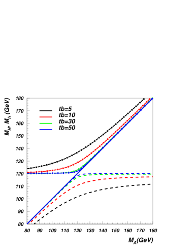
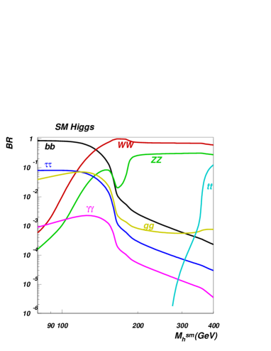
Figure 1: Left frame: Higgs spectrum in the MSSM. Lower curves indicate $M_{h}\ vs.\ M_{A}$ for indicated values of $\tan\beta$. Upper curves do likewise for $M_{H}\ vs.\ M_{A}$. Note the potential for degenerate Higgs masses near 120 GeV. Right frame: Branching ratios of the dominant decay modes of the SM Higgs boson. Results have been obtained with the program HDECAY [15] for $\alpha_{s}(M_{Z}^{2})=0.120$, $\overline{m}_{b}(m_{b})=4.22$ GeV, $m_{t}=178$ GeV.

Let us consider how the signal of a light Higgs boson could be changed in the MSSM, compared to expectations in the SM. There are several important sources of alterations in the predicted signal, some of which are interconnected.

First, the MSSM includes three neutral Higgs bosons ${\cal H}=(h,H,A)$ states. The apparent signal of a single light Higgs could be enhanced if two or three neutral Higgs species are nearly degenerate so that more than one Higgs is actually contributing to the final state being studied. The left-hand frame of Figure 1 illustrates that for Higgs masses around 120 GeV it is possible for several Higgs states to be close in mass. We take advantage of this near-degeneracy by combining the signals of the different neutral Higgs bosons when their masses are closer than the experimental resolution. Specifically, when combining the signal from $A$, $h$, and $H$, we require $|M_{A}-M_{h}|$ and/or $|M_{A}-M_{H}|$ to be less than 0.3$\sqrt{M_{A}/GeV}$ GeV, as compared to the approximate experimental resolution for the Higgs mass of $\sqrt{M_{A}/GeV}$ GeV for $\tau^{+}\tau^{-}$ or $b\bar{b}$ channels. For the Higgs mass range studied here, 0.3$\sqrt{M_{A}/GeV}$ would correspond to a fairly small mass gap of order $\sim 3-5$ GeV. For the $\gamma\gamma$ channel we do not combine the $(h,H,A)$ states but use just one, the $A\to\gamma\gamma$ process, since the experimental mass resolution for this final state could be of the order of one GeV.

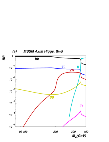
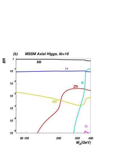
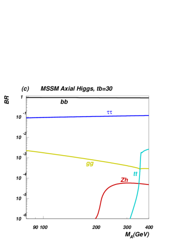
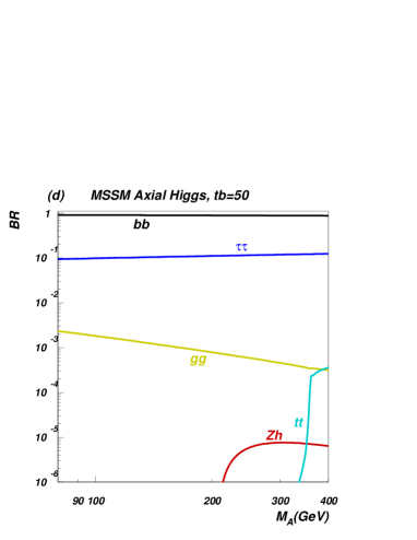
Figure 2: Branching ratios of the dominant decay modes of the MSSM CP-odd Higgs boson. Results have been obtained with the program HDECAY [15] for $\alpha_{s}(M_{Z}^{2})=0.120$, $\overline{m}_{b}(m_{b})=4.22$ GeV, $m_{t}=178$ GeV. Frames (a), (b), (c), and (d) correspond to $\tan\beta=5,10,30$ and 50, respectively.

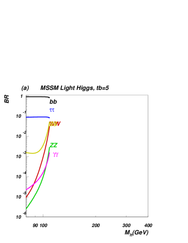
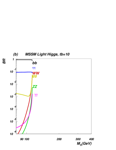
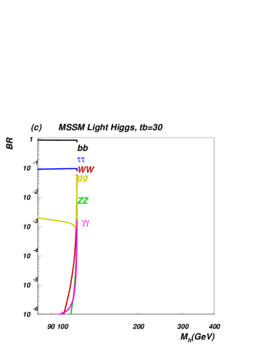
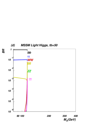
Figure 3: Branching ratios of the dominant decay modes of the MSSM Light Higgs boson. Results have been obtained with the program HDECAY [15] for $\alpha_{s}(M_{Z}^{2})=0.120$, $\overline{m}_{b}(m_{b})=4.22$ GeV, $m_{t}=178$ GeV. Frames (a), (b), (c), and (d) correspond to $\tan\beta=5,10,30$ and 50, respectively.

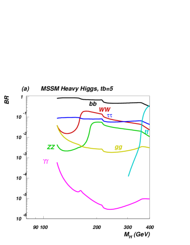
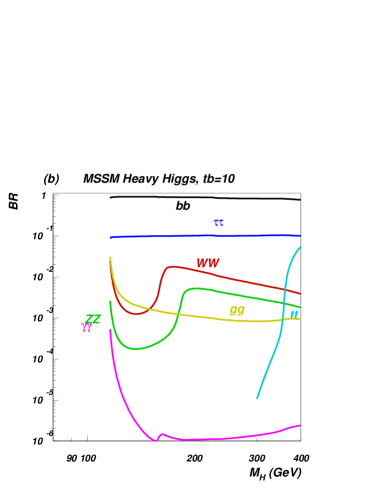
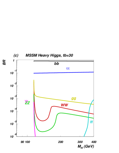
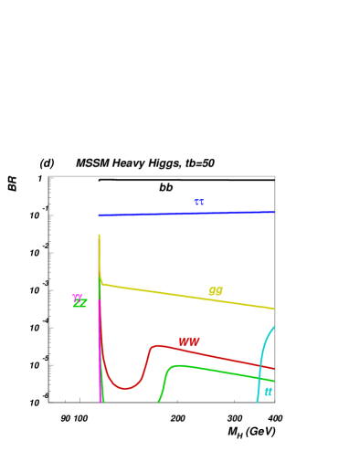
Figure 4: Branching ratios of the dominant decay modes of the MSSM Heavy Higgs boson. Results have been obtained with the program HDECAY [15] for $\alpha_{s}(M_{Z}^{2})=0.120$, $\overline{m}_{b}(m_{b})=4.22$ GeV, $m_{t}=178$ GeV. Frames (a), (b), (c), and (d) correspond to $\tan\beta=5,10,30$ and 50, respectively.

Second, the alterations of the couplings between Higgs bosons and ordinary fermions in the MSSM, which were discussed in section 2.2, can change the Higgs decay widths and branching ratios relative to those in the SM. The SM branching fractions are pictured in the right-hand frame of Figure 1 and those in the MSSM (as calculated with the HDECAY program [15]) are in Figures 2, 3, 4, and the relevant branching ratios for a 130 GeV CP-odd Higgs are given for various $\tan\beta$ in Table 1. These changes directly effect the enhancement factor for a given process, as in equation (1). When radiative effects on the masses and couplings are included, the Higgs boson production rate as well as the decay branching fractions can be substantially altered, in a non-universal way. For instance, $B(h\to\tau^{+}\tau^{-})$ could be enhanced by up to an order of magnitude due to the suppression of $B(h\to b\bar{b})$ in certain regions of parameter space [36, 37]. However, this gain in branching fraction would be offset to some degree by a reduction in Higgs production through channels involving $Y_{{\cal H}b\bar{b}}$.

Table 1: Branching ratios for a CP-odd MSSM Higgs of mass 130 GeV.

Decay	$\tan\beta=5$	$\tan\beta=10$	$\tan\beta=30$	$\tan\beta=50$
Channel
$b\overline{b}$	0.90	0.90	0.90	0.89
$c\overline{c}$	$6.5\times 10^{-5}$	$4.1\times 10^{-6}$	$5.2\times 10^{-8}$	$6.9\times 10^{-9}$
$\tau^{+}\tau^{-}$	0.095	0.096	0.099	0.10
$gg$	$7.5\times 10^{-4}$	$1.0\times 10^{-3}$	$1.3\times 10^{-3}$	$1.3\times 10^{-3}$
$\gamma\gamma$	$2.7\times 10^{-7}$	$5.4\times 10^{-7}$	$5.9\times 10^{-7}$	$5.9\times 10^{-7}$
$W^{+}W^{-}$	0	0	0	0

Third, recall that SM production of the light Higgs via gluon fusion is dominated by a top-quark loop; the large top quark mass both increases the top-Higgs coupling and suppresses the loop. In the MSSM, a large value of $\tan\beta$ enhances the bottom-Higgs coupling (eqns. (16) and (17)), making gluon fusion through a $b$-quark loop significant, and possibly even dominant over the top-quark loop contribution.

Fourth, the presence of superpartners in the MSSM gives rise to new squark-loop contributions to Higgs boson production through gluon fusion. Light squarks with masses of order 100 GeV have been argued to lead to a considerable universal enhancement (as much as a factor of five) [38, 39, 40, 41] for MSSM Higgs production compared to the SM.

Finally, enhancement of the $Y_{{\cal H}b\bar{b}}$ coupling at moderate to large $\tan\beta$ makes $b\bar{b}\to{\cal H}$ a significant means of Higgs production in the MSSM – in contrast to the SM where it is negligible. To include both production channels when looking for a Higgs decaying as ${\cal H}\to xx$, we define a combined enhancement factor

$$\kappa_{total/xx}^{\cal H} = \sigma(gg\to{\cal H}\to xx)+\sigma(bb\to{\cal H}\to xx)\over{\sigma(gg\to h_{SM}\to xx)+\sigma(bb\to h_{SM}\to xx)}$$ (18)

$$= \kappa_{gg/xx}^{\cal H}+\sigma(bb\to{\cal H}\to xx)/\sigma(gg\to h_{SM}\to xx)\over{1+\sigma(bb\to h_{SM}\to xx)/\sigma(gg\to h_{SM}\to xx)}$$

$$= \kappa_{gg/xx}^{\cal H}+\kappa_{bb/xx}^{\cal H}\sigma(bb\to h_{SM}\to xx)/\sigma(gg\to h_{SM}\to xx)\over{1+\sigma(bb\to h_{SM}\to xx)/\sigma(gg\to h_{SM}\to xx)}$$

$$\equiv [\kappa_{gg/xx}^{\cal H}+\kappa_{bb/xx}^{\cal H}R_{bb:gg}]/[{1+R_{bb:gg}}].$$

Here $R_{bb:gg}$ is the ratio of $b\bar{b}$ and $gg$ initiated Higgs boson production in the Standard Model, which can be calculated using HDECAY.

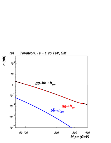
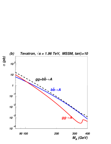
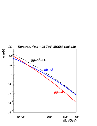
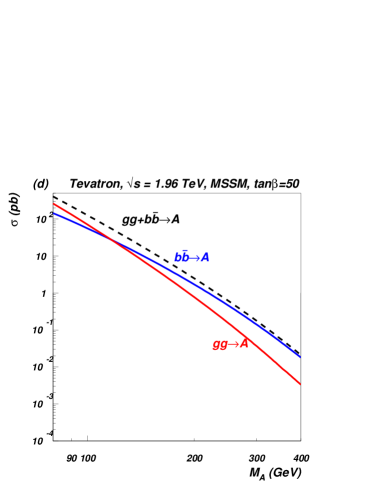
Figure 5: NLO cross sections for Higgs production via the $b\bar{b}\to{\cal H}$ and $gg\to{\cal H}$ processes (as well as their sum) for (a) the SM Higgs, and (b)-(d) the Supersymmetric axial Higgs boson with $\tan\beta=10,30$ and 50, respectively, at the Tevatron.

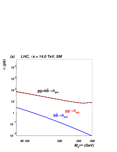
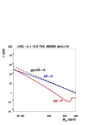
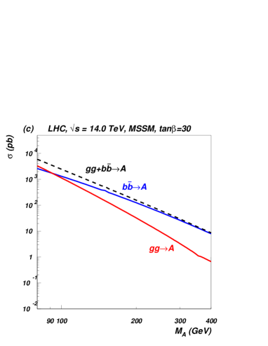
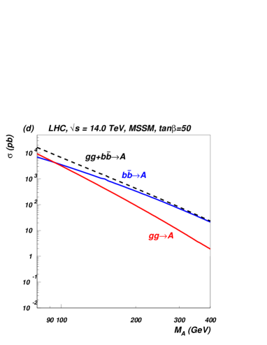
Figure 6: NLO cross sections for Higgs production via the $b\bar{b}\to{\cal H}$ and $gg\to{\cal H}$ processes (as well as their sum) for (a) the SM Higgs, and (b)-(d) the Supersymmetric axial Higgs boson with $\tan\beta=10,30$ and 50, respectively, at the LHC.

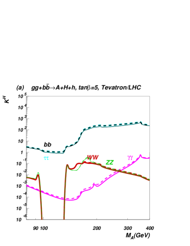
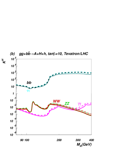
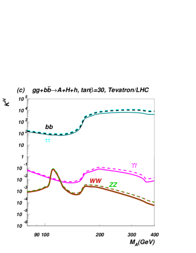
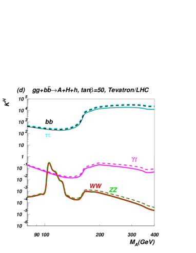
Figure 7: Enhancement factor $\kappa^{\cal H}_{tot/xx}$ for final states $xx=b\bar{b},\ \tau^{+}\tau^{-},\ WW,\ ZZ,\ \gamma\gamma$ when both $gg\to{\cal H}$ and $b\bar{b}\to{\cal H}$ are included and the signals of all three MSSM Higgs states are combined. Frames (a), (b), (c), and (d) correspond to $\tan\beta=5,10,30$ and 50, respectively, at the Tevatron (solid lines) and at the LHC (dashed lines).

3.1.2 Enhancement Factors and Cross-sections

Figure 5 (6) presents NLO cross sections at the Tevatron (LHC). For $b\bar{b}\to{\cal H}$ we are using the code of Ref. [42], while for $gg\to{\cal H}$ we use HIGLU [44] and HDECAY [15] . Frame (a) shows production of $h_{SM}$; frames (b)-(d) show production of the MSSM axial Higgs for several values of $\tan\beta$. One can see that in the MSSM the contribution from $b\bar{b}\to{\cal H}$ becomes important even for moderate values of $\tan\beta\sim 10$. For $M_{\cal H}<110-115$ GeV the contribution from $gg\to{\cal H}$ process is a bit bigger than that from $b\bar{b}\to{\cal H}$, while for $M_{\cal H}>115$ GeV $b$-quark-initiated production begins to outweigh gluon-initiated production.

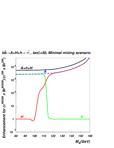
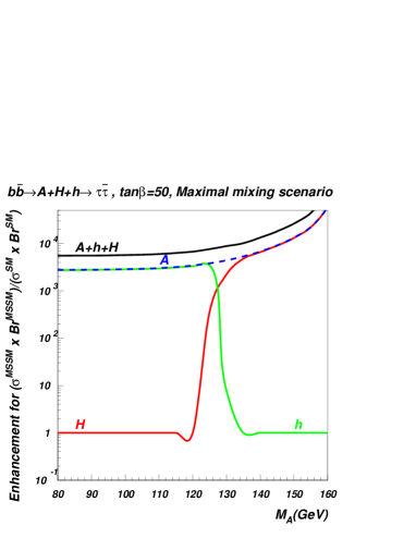
Figure 8: Enhancement factor $\kappa^{\cal H}_{bb/\tau\tau}$ (for $b\bar{b}\to H+h+A\to\tau^{+}{\tau^{-}}$) for the minimal (left) and maximal (right) mixing scenarios. In both scenarios $\kappa^{\cal H}_{bb/\tau\tau}$ is the same (within at most a few percent) for fixed $M_{A}$, $\mu$ and $M_{SUSY}$ parameters: $\kappa^{\cal H}_{bb/\tau\tau}$ is independent of the collider energy and essentially independent of the $X_{t}$ variable which describes top squark mixing.

Table 2: Enhancement factors for a 130 GeV MSSM CP-odd Higgs at the Tevatron and LHC, compared to production and decay of a SM Higgs Boson of the same mass. The $b$-quark annihilation channel has been combined with the gluon fusion channel, as described in the text. The rightmost column shows the cross-section (pb) for NLO $p\bar{p}/pp\to{\cal H}\to xx$ at Tevatron Run II/LHC; for $b\bar{b}$ and $\tau^{+}\tau^{-}$ channels the production of the $A$ is summed with that of the $h$ or $H$ if the mass gap $\Delta M_{A}=|M_{A}-M_{h}(M_{H})|$ is less than $0.3\sqrt{M_{A}}$.

Tevatron
Model	Decay mode	$\kappa^{\cal H}_{prod}$	$\kappa^{A}_{dec}$	$\kappa^{\cal H}_{tot/xx}$	Cross Section
	$b\overline{b}$	0.5	1.72	0.88	0.23 pb
$\tan\beta=5$	$\tau^{+}\tau^{-}$	0.5	1.75	0.89	0.025 pb
	$\gamma\gamma$	0.5	$1.2\times 10^{-4}$	$6.2\times 10^{-5}$	$7.0\times 10^{-8}$ pb
	$b\overline{b}$	4.9	1.72	8.5	2.3 pb
$\tan\beta=10$	$\tau^{+}\tau^{-}$	4.9	1.76	8.8	0.24 pb
	$\gamma\gamma$	4.9	$2.4\times 10^{-4}$	$5.0\times 10^{-3}$	$5.7\times 10^{-6}$
	$b\overline{b}$	42.	1.71	72	19 pb
$\tan\beta=30$	$\tau^{+}\tau^{-}$	42.	1.82	77	2.1 pb
	$\gamma\gamma$	42.	$2.7\times 10^{-4}$	$8.4\times 10^{-3}$	$9.6\times 10^{-6}$
	$b\overline{b}$	115	1.70	196	52 pb
$\tan\beta=50$	$\tau^{+}\tau^{-}$	115	1.88	217	6.0 pb
	$\gamma\gamma$	115	$2.6\times 10^{-4}$	$2.6\times 10^{-2}$	$3.0\times 10^{-5}$
LHC
Model	Decay mode	$\kappa^{\cal H}_{prod}$	$\kappa^{A}_{dec}$	$\kappa^{\cal H}_{tot/xx}$	Cross Section
	$b\overline{b}$	0.67	1.72	1.15	19.1 pb
$\tan\beta=5$	$\tau^{+}\tau^{-}$	0.67	1.75	1.17	2.01 pb
	$\gamma\gamma$	0.67	$1.2\times 10^{-4}$	$8.1\times 10^{-5}$	$5.7\times 10^{-6}$ pb
	$b\overline{b}$	6.1	1.72	10.5	173 pb
$\tan\beta=10$	$\tau^{+}\tau^{-}$	6.1	1.76	10.8	18.6 pb
	$\gamma\gamma$	6.1	$2.4\times 10^{-4}$	$5.9\times 10^{-3}$	$4.2\times 10^{-4}$
	$b\overline{b}$	52.9	1.71	90	1500 pb
$\tan\beta=30$	$\tau^{+}\tau^{-}$	52.9	1.82	96	166 pb
	$\gamma\gamma$	52.9	$2.7\times 10^{-4}$	$1.1\times 10^{-2}$	$7.5\times 10^{-4}$
	$b\overline{b}$	144	1.70	246	4078 pb
$\tan\beta=50$	$\tau^{+}\tau^{-}$	144	1.88	272	467 pb
	$\gamma\gamma$	144	$2.6\times 10^{-4}$	$3.2\times 10^{-2}$	$2.3\times 10^{-3}$

Using the Higgs branching fractions from above with these NLO cross sections for $gg\to H$ and $b\bar{b}\to H$ allows us to derive $\kappa_{total/xx}^{\cal H}$, as presented in Fig. 7 for the Tevatron and LHC. Several comments are in order. In Fig. 7(a) one can see a gap in enhancement factor for $WW$ and $ZZ$ final states at $\tan\beta=5$ for $M_{A}$ between 90-130 GeV. This is related to our procedure of combining signals from $(A,h,H)$ bosons. The $A$-boson does not couple to $WW$ or $ZZ$, while the mass gap between $h$ and $H$ is too big at low values of $\tan\beta$ to satisfy our combination criterion ($|M_{A}-M_{H,h}|<0.3\sqrt{M_{A}/GeV}$), so one cannot define an enhancement factor for this parameter region. At higher values of $\tan\beta$ there is no corresponding gap for $WW$ and $ZZ$ final states for $M_{A}$ between 90-130 GeV, however one can observe artificial peaks for $M_{A}$ between 90-130 GeV which are again related to our combination procedure. In addition, there are several “physical” kinks and peaks in the enhancement factor for various Higgs boson final states related to $WW$, $ZZ$ and top-quark thresholds which can be seen for the respective values of $M_{A}$. At very large values of $\tan\beta$ the top-quark threshold effect for the $\gamma\gamma$ enhancement factor is almost gone because the b-quark contribution dominates in the loop.

The enhancement factors and cross sections for a 130 GeV CP-odd Higgs are listed, for various values of $\tan\beta$, in Table 2. From Table 2 one can see that the enhancement factors at the Tevatron and LHC are very similar. On the other hand, the values of the total rates at the LHC are about two orders of magnitude higher than the corresponding rates at the Tevatron. One should also notice that enhancements of the $b\bar{b}$ and $\tau^{+}\tau^{-}$ signatures are very similar and they rise swiftly by a factor of 200 as $\tan\beta$ increases from 5 to 50. In contrast, the $\gamma\gamma$ signature is always strongly suppressed! This particular feature of SUSY models, as we will see below, may be important for distinguishing supersymmetric models from models with dynamical symmetry breaking.

It is important to note that combining the signal from the neutral Higgs bosons $h,A,H$ in the MSSM turns out to make our results more broadly applicable across SUSY parameter space. As discussed earlier, Figure 1(left) reveals that at moderate-to-high values of $\tan\beta$ at least two of the neutral Higgs bosons are degenerate in mass . The value of the light Higgs mass $M_{h}$ also depends on the degree of mixing between the scalar partners of the top quark; this is parameterized by the variable $A_{t}$. For a given SUSY scale, $M_{S}$, the mass $M_{h}$ takes its maximum value for $X_{t}\equiv A_{t}-\mu\cot\beta=\sqrt{6}M_{S}$ which corresponds to the “maximal mixing case” while for $X_{t}\equiv A_{t}-\mu\cot\beta=0$ we have the “minimal mixing case” and $M_{h}$ takes on its minimum value. What is interesting is that although the value of $M_{h}$ can differ significantly in the minimal and maximal mixing cases, the combined signal from all 3 Higgses at high $\tan\beta$ leads to the nearly the same (within at most few percent) enhancement factor, as shown in Figure 8. Combining the signals from $A,h,H$ has the virtue of making the enhancement factor independent of the degree of top squark mixing (for fixed $M_{A}$, $\mu$ and $M_{S}$ and medium to high values of $\tan\beta$), which greatly reduces the parameter-dependence of our results.

3.2 Technicolor

3.2.1 PNGB Production via Gluon Fusion

Single production of a technipion can occur through the axial-vector anomaly which couples the technipion to pairs of gauge bosons. For an $SU(N_{TC})$ technicolor group with technipion decay constant $F_{P}$, the anomalous coupling between the technipion and a pair of gauge bosons is given, in direct analogy with the coupling of a QCD pion to photons, by [45, 46, 47]

$$N_{TC}{\cal A}_{V_{1}V_{2}}{g_{1}g_{2}\over 8\pi^{2}F_{P}}\epsilon_{\mu\nu\lambda\sigma}k_{1}^{\mu}k_{2}^{\nu}\epsilon_{1}^{\lambda}\epsilon_{2}^{\sigma}$$ (19)

where ${\cal A}_{V_{1}V_{2}}$ is the anomaly factor, $g_{i}$ are the gauge boson couplings, and the $k_{i}$ and $\epsilon_{i}$ are the four-momenta and polarizations of the gauge bosons. The values of the anomaly factors for the lightest PNGB coupling to gluons are given in Table 3 for each model.

Table 3: Anomaly Factors for the technicolor models under study [2, 3, 33, 35, 48]

	1) one-family	2) variant one-family	3) multiscale	4) low-scale
${\cal A}_{gg}$	$\frac{1}{\sqrt{3}}$	$\frac{1}{\sqrt{6}}$	$\sqrt{2}$	$\frac{1}{\sqrt{3}}$
${\cal A}_{\gamma\gamma}$	$-\frac{4}{3\sqrt{3}}$	$\frac{16}{3\sqrt{6}}$	$\frac{4\sqrt{2}}{3}$	$\frac{34}{9}$

The rate of single technipion production in this channel is proportional to the decay width to gluons. In the technicolor models, we have

$${\Gamma(P\rightarrow gg)}={m_{P}^{3}\over 8\pi}\left(\frac{\alpha_{s}N_{TC}{\cal A}_{gg}}{2\pi F_{P}}\right)^{2}\ .$$ (20)

while in the SM, the expression looks like [13]

$${\Gamma(h\rightarrow gg)}={m_{h}^{3}\over 8\pi}\left(\frac{\alpha_{s}}{3\pi v}\right)^{2}~{},$$ (21)

in the heavy top-quark approximation. Comparing a PNGB to a SM Higgs boson of the same mass, we find the enhancement in the gluon fusion production rate is

$$\kappa_{gg\ prod}=\frac{\Gamma(P\rightarrow gg)}{\Gamma(h\rightarrow gg)}=\frac{9}{4}N_{TC}^{2}{\cal A}_{gg}^{2}\frac{v^{2}}{F_{P}^{2}}$$ (22)

The main factors influencing $\kappa_{gg\ prod}$ for a fixed value of $N_{TC}$ are the anomalous coupling to gluons and the technipion decay constant. The value of $\kappa_{gg\ prod}$ for each model (taking $N_{TC}=4$) is given in Table 4.

Table 4: Calculated enhancement factors for production at the Tevatron and LHC of a 130 GeV technipion via $gg$ alone, via $b\bar{b}$ alone, and combined. Note that the small enhancement in the $b\bar{b}$ process slightly reduces the total enhancement relative to that of $gg$ alone. In all cases, $N_{TC}=4$.

	1) one family	2) variant one-family	3) multiscale	4) low scale
$\kappa^{P}_{gg\ prod}$	48	6	1200	120
$\kappa^{P}_{bb\ prod}$	4	0.67	16	10
$\kappa^{P}_{prod}$	47	5.9	1100	120

3.2.2 Production via $b\bar{b}$ annihilation

The PNGBs couple to b-quarks courtesy of the extended technicolor interactions [30, 31] responsible for producing masses for the ordinary quarks and leptons. The extended technicolor group (of which $SU(N_{TC})$ is an unbroken subgroup) includes gauge bosons that couple to both ordinary and technicolored fermions so that the ordinary fermions can interact with the technicondensates that break the electroweak symmetry.

The rate of technipion production via $b\bar{b}$ annihilation is proportional to $\Gamma(P\to b\bar{b})$. In general, the expression for the decay of a technipion to fermions is

$${\Gamma(P\rightarrow f\overline{f})}={N_{C}\,\lambda^{2}_{f}\,m^{2}_{f}\,m_{P}\over 8\pi\,F^{2}_{P}}\,\left(1-\frac{4m_{f}^{2}}{m_{P}^{2}}\right)^{\frac{s}{2}}$$ (23)

where $N_{C}$ is 3 for quarks and 1 for leptons. The phase space exponent, $s$, is 3 for scalars and 1 for pseudoscalars; the lightest PNGB in models 1 and 4 is a scalar, while in models 2 and 3 it is assumed to be a pseudoscalar. For the technipion masses considered here, the value of the phase space factor in (23) is so close to one that the value of $s$ makes no practical difference. The factor $\lambda_{f}$ is a non-standard Yukawa coupling distinguishing leptons from quarks. Model 2 has $\lambda_{quark}=\sqrt{\frac{2}{3}}$ and $\lambda_{lepton}=\sqrt{6}$; model 3 also includes a similar factor, but with average value 1; $\lambda_{f}=1$ in models 1 and 4. Finally, it should be noted that model 2 assumes that the lightest technipion is composed only of down-type fermions and cannot decay to $c\bar{c}$; since this decay would usually have a small branching ratio and $c\bar{c}$ is not a preferred final state for Higgs searches, this has little impact.

For comparison, the decay width of the SM Higgs into b-quarks is:

$${\Gamma(h\rightarrow b\overline{b})}={3\,m^{2}_{b}\,m_{h}\over 8\pi\,v^{2}}\left(1-\frac{4m_{b}^{2}}{m_{h}^{2}}\right)^{\frac{3}{2}}$$ (24)

The production enhancement for $b\bar{b}$ annihilation is (again assuming Higgs and technipion have the same mass):

$$\kappa_{bb\ prod}=\frac{\Gamma(P\rightarrow b\overline{b})}{\Gamma(h\rightarrow b\overline{b})}={\lambda^{2}_{b}\,v^{2}\over F^{2}_{P}}\left(1-\frac{4m_{b}^{2}}{m_{h}^{2}}\right)^{\frac{s-3}{2}}$$ (25)

The value of $\kappa_{bb\ prod}$ (shown in Table 4) is controlled by the size of the technipion decay constant.

We see from Table 4 that $\kappa_{bb\ prod}$ is at least one order of magnitude smaller than $\kappa_{gg\ prod}$ in each model. Taking the ratio of equations (22) and (25)

$$\frac{\kappa_{gg\ prod}}{\kappa_{bb\ prod}}=\frac{9}{4}N_{TC}^{2}{\cal A}_{gg}^{2}\lambda_{b}^{-2}\left(1-\frac{4m_{b}^{2}}{m_{h}^{2}}\right)^{\frac{3-s}{2}}$$ (26)

we see that the larger size of $\kappa_{gg\ prod}$ is due to the factor of $N_{TC}^{2}$ coming from the fact that gluons couple to a technipion via a techniquark loop. The extended technicolor (ETC) interactions coupling $b$-quarks to a technipion have no such enhancement.

In addition, the production cross-section for a SM Higgs boson via $b\bar{b}$ annihilation is 2 to 3 orders of magnitude smaller than that for gluon fusion at the Tevatron [49] and LHC [44]. With a smaller SM cross-section and a smaller enhancement factor, it is clear that technipion production via $b\bar{b}$ annihilation is essentially negligible at these hadron colliders. Nonetheless, to be conservative, we include the $b\bar{b}$ production channel because it tends to slightly reduce the production enhancement factor.

Using the combined enhancement factor definition of eqn. (18), and recalling that $\kappa_{dec}$ is the same for both colliders, we find that the small differences due to the values of $R_{bb:gg}$ do not give a noticable difference between the values of $\kappa^{P}_{total/xx}$ at the Tevatron and LHC; the production enhancement factors quoted in Table 4 apply to both colliders.

3.2.3 Decays

The decay width of a light technipion into gluons or fermion/anti-fermion pairs has been discussed above. Since the technipions we are studying do not decay to $W$ bosons and their decay to $Z$ bosons through the axial vector anomaly is negligible in the interesting mass range, the remaining possibility is a decay to photons. Again, this proceeds through the axial vector anomaly (cf. eqn. (19)) and the anomaly factors ${\cal A}_{\gamma\gamma}$ are shown in Table 3.

We now calculate the technipion branching ratios from the above information, taking $N_{TC}=4$. The values are essentially independent of the size of $M_{P}$ within the range 120 GeV - 160 GeV; the branching fractions for $M_{P}=130$ GeV are shown in Table 5. The branching ratios for the SM Higgs at NLO are given for comparison; they were calculated using HDECAY [15]. Note that, in contrast to the technipions, a SM Higgs in this mass range already has a noticeable decay rate to off-shell vector bosons.

Table 5: Branching ratios of Technipions/Higgs of mass 130 GeV

Decay	1) one family	2) variant	3) multiscale	4) low scale	SM Higgs
Channel		one family
$b\overline{b}$	0.60	0.53	0.23	0.60	0.53
$c\overline{c}$	0.05	0	0.03	0.05	0.02
$\tau^{+}\tau^{-}$	0.03	0.25	0.01	0.03	0.05
$gg$	0.32	0.21	0.73	0.32	0.07
$\gamma\gamma$	$2.7\times 10^{-4}$	$2.9\times 10^{-3}$	$6.1\times 10^{-4}$	$6.4\times 10^{-3}$	$2.2\times 10^{-3}$
$W^{+}W^{-}$	0	0	0	0	0.29

Comparing the technicolor and SM branching ratios in Table 5, we see immediately that all decay enhancements, except to the $gg$ mode, are generally of order one and therefore much smaller than the production enhancements. Decays to $b\bar{b}$ are slightly enhanced, if at all. Decays to $c\bar{c}$ are enhanced in our tree-level calculations – but note that it is higher-order corrections that suppress this mode for the SM Higgs; in any case, this is not a primary discovery channel. Decays to $\tau$ leptons are slightly suppressed in general; again, the comparison of tree-level technicolor and loop-level SM Higgs calculations may be a factor here. Model 2 is an exception; its unusual Yukawa couplings yield a decay enhancement in the $\tau^{+}\tau^{-}$ channel of order the technipion’s (low) production enhancement. In the $\gamma\gamma$ channel, the decay enhancement strongly depends on the group-theoretical structure of the model, through the anomaly factor. Table 6 includes the decay enhancements $\kappa^{P}_{dec}$ for the most experimentally promising search channels.

Table 6: Enhancement Factors for 130 GeV technipions produced at the Tevatron and LHC, compared to production and decay of a SM Higgs Boson of the same mass. The slight suppression of $\kappa^{P}_{prod}$ due to the b-quark annihilation channel has been included. The rightmost column shows the cross-section (pb) for $p\bar{p}/pp\to P\to xx$ at Tevatron Run II/LHC.

Tevatron
Model	Decay mode	$\kappa^{P}_{prod}$	$\kappa^{P}_{dec}$	$\kappa^{P}_{tot/xx}$	Cross Section
	$b\overline{b}$	47	1.1	52	14 pb
1) one family	$\tau^{+}\tau^{-}$	47	0.6	28	0.77 pb
	$\gamma\gamma$	47	0.12	5.6	$6.4\times 10^{-3}$ pb
	$b\overline{b}$	5.9	1	5.9	1.8 pb
2) variant	$\tau^{+}\tau^{-}$	5.9	5	30	0.84 pb
one family	$\gamma\gamma$	5.9	1.3	7.7	$8.7\times 10^{-3}$ pb
	$b\overline{b}$	1100	0.43	470	130 pb
3) multiscale	$\tau^{+}\tau^{-}$	1100	0.2	220	6.1 pb
	$\gamma\gamma$	1100	0.27	300	0.34 pb
	$b\overline{b}$	120	1.1	130	36 pb
4) low scale	$\tau^{+}\tau^{-}$	120	0.6	72	2 pb
	$\gamma\gamma$	120	2.9	350	0.4 pb
LHC
Model	Decay mode	$\kappa^{P}_{prod}$	$\kappa^{P}_{dec}$	$\kappa^{P}_{tot/xx}$	Cross Section
	$b\overline{b}$	47	1.1	52	890 pb
1) one family	$\tau^{+}\tau^{-}$	47	0.6	28	48 pb
	$\gamma\gamma$	47	0.12	5.6	0.4 pb
	$b\overline{b}$	5.9	1	5.9	100 pb
2) variant	$\tau^{+}\tau^{-}$	5.9	5	30	52 pb
one family	$\gamma\gamma$	5.9	1.3	7.7	0.55 pb
	$b\overline{b}$	1100	0.43	473	8000 pb
3) multiscale	$\tau^{+}\tau^{-}$	1100	0.2	220	380 pb
	$\gamma\gamma$	1100	0.27	300	22 pb
	$b\overline{b}$	120	1.1	130	2200 pb
4) low scale	$\tau^{+}\tau^{-}$	120	0.6	72	120 pb
	$\gamma\gamma$	120	2.9	350	25 pb

3.2.4 Enhancement Factors and Cross-Sections

Our results for the Tevatron Run II and LHC production enhancements (including both $gg$ fusion and $b\bar{b}$ annihilation), decay enhancements, and overall enhancements of each technicolor model relative to the SM are shown in Table 6 for a technipion or Higgs mass of 130 GeV. Multiplying $\kappa^{P}_{tot/xx}$ by the cross-section for SM Higgs production via gluon fusion [44] yields an approximate technipion production cross-section, as shown in the right-most column of Table 6.

In each technicolor model, the main enhancement of the possible technipion signal relative to that of an SM Higgs arises at production, making the size of the technipion decay constant the most critical factor in determining the degree of enhancement for fixed $N_{TC}$.

Each decay enhancement is in general of order 1, making it significantly smaller than the typical production enhancement. In model 3 where the decay “enhancement” is actually a suppression, the decay factor is 3 orders of magnitude smaller than the production enhancement. We find that $P\to b\bar{b}$ is very similar to $h_{SM}\to b\bar{b}$. The decay $P\to\tau^{+}\tau^{-}$ generally has a suppressed rate relative to SM expectations; again, this may relate to comparing leading technicolor and NLO SM results. An exception is model 2, where the special structure of the Yukawa coupling leads to a $\tau^{+}\tau^{-}$ decay enhancement of the same order as the production enhancement. The $P\to\gamma\gamma$ decay enhancement factor depends strongly on the group-theoretic structure of the model through the anomaly factor, ranging from a distinct enhancement in model 4 to a factor-of-10 suppression in model 1.

4 Interpretation

We are ready to put our results in context. The large QCD background for $q\bar{q}$ states of any flavor makes the tau-lepton-pair and di-photon final states the most promising for exclusion or discovery of the Higgs-like states of the MSSM or technicolor. We now illustrate how the size of the enhancement factors for these two final states vary over the parameter spaces of these theories at the Tevatron and LHC. We use this information to display the likely reach of each experiment in each of these standard Higgs search channels. Then, we compare the signatures of the MSSM Higgs bosons and the various technipions to see how one might tell these states apart from one another.

4.1 Visibility of MSSM Higgs Bosons

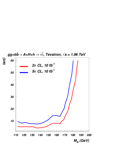
Figure 9: Results for $gg+b\bar{b}\to h+H+A\to\tau^{+}\tau^{-}$ at Tevatron Run II. Left frame: Selected contours of given enhancement factor values $\kappa^{\cal H}_{total/\tau\tau}$ in the MSSM. Right frame: Predicted Tevatron reach, based on the $h_{SM}\to\tau^{+}\tau^{-}$ studies of [9], in the MSSM parameter space. Lower contour is a $2\sigma$ exclusion contour; upper contour is a $5\sigma$ discovery contour.

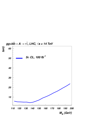
Figure 10: Results for $gg+b\bar{b}\to h+H+A\to\tau^{+}\tau^{-}$ at LHC. Left frame: Selected contours of given enhancement factor values $\kappa^{\cal H}_{total/\tau\tau}$ in the MSSM. Right frame: Predicted LHC reach, based on the $h_{SM}\to\tau^{+}\tau^{-}$ studies of [10], in the MSSM parameter space.

The left-hand frame of Figure 9 displays contours of enhancement factors of 2, 10, 100 and 1000 for the process $gg+b\bar{b}\to h+A+H\to\tau^{+}\tau^{-}$ in the MSSM at the Tevatron. We see that the enhancement factors grow dramatically as either $\tan\beta$ or $M_{A}$ becomes large. These results are consistent with those of [9]. The large increase in the enhancement factor for large values of $M_{A}$ takes place because the Standard Model $Br[H\to\tau\tau(b\bar{b})]$ decreases sharply when the $WW$ and $ZZ$ decay channels open, while in the MSSM the $Br[A\to\tau\tau(b\bar{b})]$ in the high $\tan\beta$ regime hardly changes.

In the right-hand frame of the same figure, we summarize the Tevatron’s ability to explore the MSSM parameter space (in terms of both a $2\sigma$ exclusion curve and a $5\sigma$ discovery curve) using the process $gg+b\bar{b}\to h+A+H\to\tau^{+}\tau^{-}$. Translating the enhancement factors above into this reach plot draws on the results of [9]. As the $M_{A}$ mass increases up to about 140 GeV, the opening of the $W^{+}W^{-}$ decay channel drives the $\tau^{+}\tau^{-}$ branching fraction down, and increases the $\tan\beta$ value required to make Higgses visible in the $\tau^{+}\tau^{-}$ channel. At still larger $M_{A}$, a very steep drop in the gluon luminosity (and the related $b$-quark luminosity) at large $x$ reduces the phase space for ${\cal H}$ production. Therefore for $M_{A}>$170 GeV, Higgs bosons would only be visible at very high values of $\tan\beta$.

Figure 10 presents a qualitatively similar picture for LHC, based on the studies of $h_{SM}\to\tau^{+}\tau^{-}$ of [10]. The main differences compared to the Tevatron are that the required value of $\tan\beta$ at the LHC is lower for a given $M_{A}$ and it does not climb steeply for $M_{A}>$170 GeV because there is much less phase space suppression.

It is important to notice that both, Tevatron and LHC, could observe MSSM Higgs bosons in the $\tau^{+}\tau^{-}$ channel even for moderate values of $\tan\beta$ for $M_{A}\lesssim 200$ GeV, because of significant enhancement of this channel. However the $\gamma\gamma$ channel is so suppressed that even the LHC will not be able to observe it in any point of the $M_{A}<200$ GeV parameter space studied in this paper!

4.2 Visibility of Technipions

In Section 3.2 we found a distinct enhancement of the $P$ signal in both the $\tau^{+}\tau^{-}$ and $\gamma\gamma$ search channels for each of the technicolor models studied. As illustrated in the left frame of Figure 11, the available enhancement is well above what is required to render the $P$ of any of these models visible in the $\tau^{+}\tau^{-}$ channel at the Tevatron. Likewise, the right frame of that figure shows that in the $\gamma\gamma$ channel at the Tevatron the technipions of models 3 and 4 will be observable at the $5\sigma$ level while model 2 is subject to exclusion at the $2\sigma$ level. The situation at the LHC is even more promising: Figure 12 shows that all four models could be observable at the $5\sigma$ level in both the $\tau^{+}\tau^{-}$ (left frame) and $\gamma\gamma$ (right frame) channels.

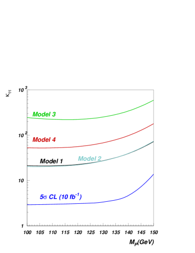
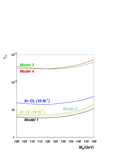
Figure 11: Total enhancement factor for each technicolor model as a function of technipion mass and assuming the final state is a tau pair (left frame) or photon pair (right frame). The $5\sigma$ discovery and $2\sigma$ exclusion curves indicate the required enhancement factor for a Higgs-like particle at Tevatron Run II when the final state is $\tau^{+}\tau^{-}$ [9] (left frame) or $\gamma\gamma$ [11](right frame).

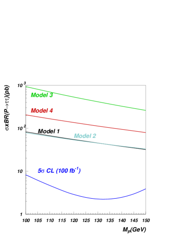
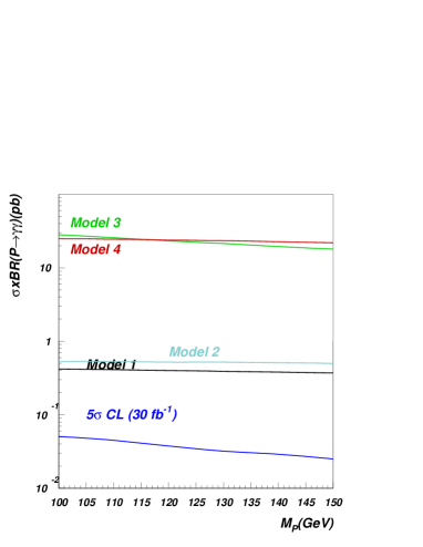
Figure 12: $\sigma\times Br$ for each technicolor model plotted as a function of technipion mass and assuming the final state is a tau($\gamma$) pair – left(right) at LHC. The lowest curve is the $\sigma\times Br$ required to make a Higgs-like particle visible ($5\sigma$ discovery) in $\tau^{+}\tau^{-}$ [10] or in $\gamma\gamma$ [12] at LHC.

4.3 Distinguishing the MSSM from Technicolor

In the previous section we have shown that that the Tevatron and LHC have the potential to observe the light (pseudo) scalar states characteristic of both supersymmetry and models of dynamical symmetry breaking. For both classes of models, the $\tau^{+}\tau^{-}$ channel is enhanced and could be used for discovery of the light Higgs-like states.

Once a supposed light “Higgs boson” is observed in a collider experiment, an immediate important task will be to identify the new state more precisely, i.e. to discern “the meaning of Higgs” in this context. Comparison of the enhancement factors for different channels will aid in this task. Our study has shown that comparison of the $\tau^{+}\tau^{-}$ and $\gamma\gamma$ channels can be particularly informative in distinguishing supersymmetric from dynamical models. In the case of supersymmetry, when the $\tau^{+}\tau^{-}$ channel is enhanced, the $\gamma\gamma$ channel is suppressed, and this suppression is strong enough that even the LHC would not observe the $\gamma\gamma$ signature. In contrast, for the dynamical symmetry breaking models studied we expect simultaneous enhancement of both the $\tau^{+}\tau^{-}$ and $\gamma\gamma$ channels. The enhancement of the $\gamma\gamma$ channel is so significant, that even at the Tevatron we may observe technipions via this signature at the $5\sigma$ level for Models 3 and 4, while Model 2 could be excluded at 95% CL at the Tevatron. The LHC collider, which will have better sensitivity to the signatures under study, will be able to observe all four models of dynamical symmetry breaking studied here in the $\gamma\gamma$ channel, and can therefore distinguish more conclusively between the supersymmetric and dynamical models.

We also would like to stress an important difference between two class of models in their production mechanisms. In supersymmetry the $b\bar{b}$ fusion process is likely to be as important as the $gg$ fusion mechanism (see Figure 6) in contributing to the total production cross section. In technicolor models, however, the $b\bar{b}$ fusion contribution to technipion production is likely to be negligible. This difference could be revealed, in principle, by looking at other (exclusive or semi-exclusive) processes: in case of supersymmetry, for example, one would expect significant enhancement of Higgs boson production associated with $b$-quarks.

5 Conclusions

In this paper we have shown that searches for a light Standard Model Higgs boson at Tevatron Run II and CERN LHC have the power to provide significant information about important classes of physics beyond the Standard Model. We demonstrated that the new scalar and pseudo-scalar states predicted in both supersymmetric and dynamical models can have enhanced visibility in standard $\tau^{+}\tau^{-}$ and $\gamma\gamma$ search channels, making them potentially discoverable at both the Tevatron Run II and the CERN LHC. The enhancement arises largely from increases in the production rate; we showed that the model parameters exerting the largest influence on the enhancement size are $\tan\beta$ in the case of the MSSM and $N_{TC}$ and $F_{P}$ in the case of dynamical symmetry breaking. At the same time, the ${\cal H}\to W^{+}W^{-}$ decay pathway is suppressed in the models studied here by at least an order of magnitude, compared to Standard Model expectations. In comparing the key signals for the non-standard scalars across models, we were able to show how one could start to identify which state has actually been found by a standard Higgs search. In particular, we investigated the likely mass reach of the Higgs search in $pp/p\bar{p}\to{\cal H}\to\tau^{+}\tau^{-}$ for each kind of non-standard scalar state, and we demonstrated that $pp\,\ \,p\bar{p}\to{\cal H}\to\gamma\gamma$ may cleanly distinguish the scalars of supersymmetric models from those of dynamical models.

6 Acknowledgments

We thank M. Spira and R. Harlander for discussions, C.-P. Yuan for providing the code from Ref. [42], and a very thorough referee for a close reading of the manuscript. This work was supported in part by the U.S. National Science Foundation under awards PHY-0354838 (A. Belyaev) and PHY-0354226 (R. S. Chivukula and E. H. Simmons). A. Blum is supported in part by a scholarship from the German National Academic Foundation (Studienstiftung des deutschen Volkes).

References

- [1] G. Rupak and E. H. Simmons, Phys. Lett. B 362, 155 (1995) [arXiv:hep-ph/9507438].
- [2] V. Lubicz and P. Santorelli, Nucl. Phys. B 460, 3 (1996) [arXiv:hep-ph/9505336].
- [3] K. R. Lynch and E. H. Simmons, Phys. Rev. D 64, 035008 (2001) [arXiv:hep-ph/0012256].
- [4] R. Barate et al. [ALEPH Collaboration], Phys. Lett. B 565, 61 (2003) [arXiv:hep-ex/0306033].
- [5] P. Bechtle [LEP Collaboration], Eur. Phys. J. C 33 (2004) S723 [arXiv:hep-ex/0401007].
- [6] G. L. Kane, T. T. Wang, B. D. Nelson and L. T. Wang, Phys. Rev. D 71, 035006 (2005) [arXiv:hep-ph/0407001].
- [7] G. Abbiendi et al. [OPAL Collaboration], Eur. Phys. J. C 40, 317 (2005) [arXiv:hep-ex/0408097].
- [8] G. Sguazzoni, Acta Phys. Slov. 55, 93 (2005) [arXiv:hep-ph/0411096].
- [9] A. Belyaev, T. Han and R. Rosenfeld, JHEP 0307, 021 (2003) [arXiv:hep-ph/0204210].
- [10] D. Cavalli et al., arXiv:hep-ph/0203056.
- [11] S. Mrenna and J. D. Wells, Phys. Rev. D 63 (2001) 015006 [arXiv:hep-ph/0001226].
- [12] R. Kinnunen, S. Lehti, A. Nikitenko and P. Salmi, J. Phys. G 31, 71 (2005) [arXiv:hep-ph/0503067].
- [13] J. F. Gunion, H. E. Haber, G. L. Kane and S. Dawson, SCIPP-89/13
- [14] J. F. Gunion, H. E. Haber, G. L. Kane and S. Dawson, arXiv:hep-ph/9302272.
- [15] A. Djouadi, J. Kalinowski and M. Spira, Comput. Phys. Commun. 108, 56 (1998) [arXiv:hep-ph/9704448].
- [16] G.. ’t Hooft in G.’t Hooft, et. al., “Recent Developments In Gauge Theories. Proceedings, Nato Advanced Study Institute, Cargese, France, August 26 - September 8, 1979,” New York, USA Plenum (1980).
- [17] E. Witten, Nucl. Phys. B 188, 513 (1981).
- [18] S. Dimopoulos and H. Georgi, Nucl. Phys. B 193, 150 (1981).
- [19] K. G. Wilson, Phys. Rev. B 4, 3174 (1971).
- [20] K. G. Wilson and J. B. Kogut, Phys. Rept. 12, 75 (1974).
- [21] S. Dawson, arXiv:hep-ph/9612229.
- [22] H. Murayama, Prepared for Theoretical Advanced Study Institute in Elementary Particle Physics (TASI 2000): Flavor Physics for the Millennium, Boulder, Colorado, 4-30 Jun 2000
- [23] E. Boos, A. Djouadi, M. Muhlleitner and A. Vologdin, Phys. Rev. D 66, 055004 (2002) [arXiv:hep-ph/0205160].
- [24] C. T. Hill and E. H. Simmons, Phys. Rept. 381, 235 (2003) [Erratum-ibid. 390, 553 (2004)] [arXiv:hep-ph/0203079].
- [25] G. W. Anderson, D. J. Castano and A. Riotto, Phys. Rev. D 55, 2950 (1997) [arXiv:hep-ph/9609463].
- [26] H. Murayama and M. E. Peskin, Ann. Rev. Nucl. Part. Sci. 46, 533 (1996) [arXiv:hep-ex/9606003].
- [27] L. Susskind, Phys. Rev. D 20, 2619 (1979).
- [28] S. Weinberg, Phys. Rev. D 13, 974 (1976).
- [29] S. Weinberg, Phys. Rev. D 19, 1277 (1979).
- [30] S. Dimopoulos and L. Susskind, Nucl. Phys. B 155, 237 (1979).
- [31] E. Eichten and K. D. Lane, Phys. Lett. B 90, 125 (1980).
- [32] E. Farhi and L. Susskind, Phys. Rept. 74, 277 (1981).
- [33] R. Casalbuoni, A. Deandrea, S. De Curtis, D. Dominici, R. Gatto and J. F. Gunion, Nucl. Phys. B 555, 3 (1999) [arXiv:hep-ph/9809523].
- [34] K. D. Lane and M. V. Ramana, Phys. Rev. D 44, 2678 (1991).
- [35] K. D. Lane, Phys. Rev. D 60, 075007 (1999) [arXiv:hep-ph/9903369].
- [36] M. Carena, S. Mrenna and C. E. M. Wagner, Phys. Rev. D 60, 075010 (1999) [arXiv:hep-ph/9808312].
- [37] M. Carena, S. Mrenna and C. E. M. Wagner, Phys. Rev. D 62, 055008 (2000) [arXiv:hep-ph/9907422].
- [38] S. Dawson, A. Djouadi and M. Spira, Phys. Rev. Lett. 77, 16 (1996) [arXiv:hep-ph/9603423].
- [39] R. V. Harlander and M. Steinhauser, next-to-leading Phys. Lett. B 574, 258 (2003) [arXiv:hep-ph/0307346].
- [40] R. Harlander and M. Steinhauser, Phys. Rev. D 68, 111701 (2003) [arXiv:hep-ph/0308210].
- [41] R. V. Harlander and M. Steinhauser, JHEP 0409, 066 (2004) [arXiv:hep-ph/0409010].
- [42] C. Balazs, H. J. He and C. P. Yuan, Phys. Rev. D 60, 114001 (1999) [arXiv:hep-ph/9812263].
- [43] R. V. Harlander and W. B. Kilgore, Phys. Rev. D 68, 013001 (2003) [arXiv:hep-ph/0304035].
- [44] M. Spira, Nucl. Instrum. Meth. A 389, 357 (1997) [arXiv:hep-ph/9610350].
- [45] S. Dimopoulos, S. Raby and G. L. Kane, Nucl. Phys. B 182, 77 (1981).
- [46] J. R. Ellis, M. K. Gaillard, D. V. Nanopoulos and P. Sikivie, Nucl. Phys. B 182, 529 (1981).
- [47] B. Holdom, Phys. Rev. D 24, 157 (1981).
- [48] R. S. Chivukula, R. Rosenfeld, E. H. Simmons and J. Terning, arXiv:hep-ph/9503202.
- [49] M. Carena et al. [Higgs Working Group Collaboration], arXiv:hep-ph/0010338.
- [50] A. Djouadi, arXiv:hep-ph/0412238.
- [51] M. Spira, arXiv:hep-ph/9810289.