Global analysis of three-flavor neutrino masses and mixings

Abstract

We present a comprehensive phenomenological analysis of a vast amount of data from neutrino flavor oscillation and non-oscillation searches, performed within the standard scenario with three massive and mixed neutrinos, and with particular attention to subleading effects. The detailed results discussed in this review represent a state-of-the-art, accurate and up-to-date (as of August 2005) estimate of the three-neutrino mass-mixing parameters.

1 Introduction

Neutrinos provide, on a macroscopic scale, the realization of two key concepts of quantum mechanics: linear superposition of states and noncommuting operators. In fact, there is compelling experimental evidence [1] that the three known neutrino states with definite flavor ($\nu_{e}$, $\nu_{\mu}$ and $\nu_{\tau}$) are linear combinations of states with definite mass $\nu_{i}$ ($i=1,2,3$), and that the Hamiltonian of neutrino propagation in vacuum [2] and matter [3, 4, 5] does not commute with flavor. The effects of flavor nonconservation (“oscillations”) take place on macroscopic distances, for typical ultrarelativistic neutrinos. The evidence for such effects comes from a series of experiments performed during about four decades of research with very different neutrino beams and detection techniques: the solar neutrino [6] experiments Homestake [7], Kamiokande [8], SAGE [9], GALLEX-GNO [10, 11, 12], Super-Kamiokande (SK) [13, 14] and Sudbury Neutrino Observatory (SNO) [15, 16, 17]; the long-baseline reactor neutrino [18] experiment KamLAND [19, 20, 21]; the atmospheric neutrino [22] experiments Kamiokande [23], Super-Kamiokande [24, 25, 26], MACRO [27], and Soudan-2 [28]; and the long-baseline accelerator neutrino [29] experiment KEK-to-Kamioka (K2K) [30, 31].

Together with the null results from the CHOOZ [32] (and Palo Verde [33]) short-baseline reactor experiments, the above oscillation data provide stringent constraints on the basic parameters governing the quantum aspects of neutrino propagation, namely, the superposition coefficients between flavor and mass states (i.e., the neutrino mixing matrix), the energy levels of the Hamiltonian in vacuum (i.e., the splittings between squared neutrino masses), and the analogous levels in matter (i.e., the neutrino interaction energies). The energy levels at rest (i.e., the absolute neutrino masses) are being probed by different, non-oscillation searches: beta decay experiments [34, 35, 36], neutrinoless double beta decay searches ($0\nu 2\beta$) [37, 38, 39], and precision cosmology [40, 41, 42, 43, 44]. Current non-oscillation data provide only upper limits on neutrino masses, except for the claim by part of the Heidelberg-Moscow experimental collaboration [45, 46, 47], whose possible $0\nu 2\beta$ signal would imply a lower bound on neutrino masses.

A highly nontrivial result emerging from these different neutrino data sample is their consistency, at a very detailed level, with the simplest extension of the standard electroweak model needed to accommodate nonzero neutrino masses and mixings, namely, with a scenario where the three known flavor states $\nu_{e,\mu,\tau}$ are mixed with only three mass states $\nu_{1,2,3}$, no other states or new neutrino interactions being needed. This “standard three-neutrino framework” (as recently reviewed, e.g., in [48, 49, 50, 51, 52, 53, 54, 55, 56, 57]) appears thus as a new paradigm of particle and astroparticle physics, which will be tested, refined, and possibly challenged by a series of new, more sensitive experiments planned for the next few years or even for the next decades [58, 59]. The first challenge might actually come very soon from the running MiniBooNE experiment [60], which is probing the only piece of data at variance with the standard three-neutrino framework, namely, the controversial result of the Liquid Scintillator Neutrino Experiment (LSND) [61].

In this review we focus on the current status of the standard three-neutrino framework and on the neutrino mass and mixing parameters which characterize it, as derived from a comprehensive, state-of-the-art analysis of a large amount of oscillation and nonoscillation neutrino data (as available in August 2005). All the results and figures shown in the review are either new or updated or improved in various ways, with respect to our previous publications in the field of neutrino phenomenology. In this sense we have tried to be as complete as possible, so as to present a self-consistent overview of the current status of the three-neutrino mass-mixing parameters. While we aimed at obtaining technically accurate and complete results, we have not aimed at being bibliographically complete; we refer the reader to [18, 22, 38, 50, 53, 62, 63, 64, 65, 66, 67, 68, 69, 70, 71, 72, 73, 74, 75, 76, 77, 78, 79] for an incomplete list of excellent reviews with rich bibliographies of old and recent neutrino papers.

2 Notation

While for quark mixing a standard notation and parametrization has emerged [1], this is not (yet) the case for (some) neutrino mass and mixing parameters. In this section we define and motivate the conventions used hereafter.

2.1 Mixing angles and CP-violating phase

At the lagrangian level, the left-handed neutrino fields with definite flavors $\nu_{\alpha L}$ $(\alpha=e,\mu,\tau)$ are assumed to be linear superpositions of the neutrino fields with definite masses $\nu_{iL}$ $(i=1,2,3)$, through a unitary complex matrix $U_{\alpha i}$:

$$\nu_{\alpha L}=\sum_{i=1}^{3}U_{\alpha i}\,\nu_{iL}\ .$$ (1)

This convention implies [62, 80] that one-particle neutrino states $|\nu\rangle$ are instead related by $U^{*}$ (see, e.g., [1, 81]),

$$|\nu_{\alpha}\rangle=\sum_{i=1}^{3}U_{\alpha i}^{*}|\nu_{i}\rangle\ .$$ (2)

A common parameterization [81] for the matrix $U$ is:

$$U=O_{23}\Gamma_{\delta}O_{13}\Gamma_{\delta}^{\dagger}O_{12}\ ,$$ (3)

where the $O_{ij}$’s are real Euler rotations with angles $\theta_{ij}\in[0,\pi/2]$ [82], while $\Gamma_{\delta}$ embeds a CP-violating phase $\delta\in[0,2\pi]$,

$$\Gamma_{\delta}=\mathrm{diag}(1,1,e^{+i\delta})\ .$$ (4)

Notice that the above definitions imply $\mathrm{det}(U)=+1$, which may be a useful property in some theoretical contexts [83].

By considering $\Gamma_{\delta}O_{13}\Gamma_{\delta}^{\dagger}$ as a single (complex) rotation, this parametrization coincides with the one recommended (together with Eq. (2)) in the Review of Particle Properties [1],

$$U=\left(\begin{array}[]{ccc}1&0&0\\ 0&c_{23}&s_{23}\\ 0&-s_{23}&c_{23}\end{array}\right)\left(\begin{array}[]{ccc}c_{13}&0&s_{13}e^{-i\delta}\\ 0&1&0\\ -s_{13}e^{i\delta}&0&c_{13}\end{array}\right)\left(\begin{array}[]{ccc}c_{12}&s_{12}&0\\ -s_{12}&c_{12}&0\\ 0&0&1\end{array}\right)$$ (5)

where $c_{ij}=\cos\theta_{ij}$ and $s_{ij}=\sin\theta_{ij}$.

Other conventions sometimes used in the literature involve $U$ instead of $U^{*}$ in Eq. (2), or $-\delta$ instead of $+\delta$ in Eq. (4), or only one CP-violating factor (either $\Gamma_{\delta}$ or $\Gamma_{\delta}^{\dagger}$, not both) in Eq. (3), or a combination of the above. In our opinion such alternatives, although legitimate, do not bring particular advantages over the above convention.

For the sake of simplicity, the phase $\delta$ will not be considered in full generality in this work. Numerical examples will refer, when needed, only to the two inequivalent CP-conserving cases, namely, $e^{i\delta}=\pm 1$. In these two cases, the mixing matrix takes a real form $U_{\mathrm{CP}}$,

$$U_{\mathrm{CP}}=\left(\begin{array}[]{ccc}c_{13}c_{12}&s_{12}c_{13}&\pm s_{13}\\ -s_{12}c_{23}\mp s_{23}s_{13}c_{12}&c_{23}c_{12}\mp s_{23}s_{13}s_{12}&s_{23}c_{13}\\ s_{23}s_{12}\mp s_{13}c_{23}c_{12}&-s_{23}c_{12}\mp s_{13}s_{12}c_{23}&c_{23}c_{13}\end{array}\right)\ ,$$ (6)

where the upper (lower) sign refers to $\delta=0$ ($\delta=\pi$). The two cases are formally related by the replacement $s_{13}\to-s_{13}$. In any case, CP violation effects do not affect at all solar and reactor oscillation searches, where the indistinguishability of $\nu_{\mu}$ and $\nu_{\tau}$ in the final state allows to rotate away both the angle $\theta_{23}$ and the CP phase $\delta$ from the parameter space, even in the presence of matter effects (see, e.g., [84]).

2.2 Masses, splittings and hierarchies

The current neutrino phenomenology implies that the three-neutrino mass spectrum $\{m_{i}\}_{i=1,2,3}$ is formed by a “doublet” of relatively close states and by a third “lone” neutrino state, which may be either heavier than the doublet (“normal hierarchy,” NH) or lighter (“inverted hierarchy,” IH). In the most frequently adopted labeling of such states, the lightest (heaviest) neutrino in the doublet is called $\nu_{1}$ ($\nu_{2}$), so that their squared mass difference is

$$\delta m^{2}=m^{2}_{2}-m^{2}_{1}>0$$ (7)

by convention. The lone state is then labeled as $\nu_{3}$, and the physical sign of $m^{2}_{3}-m^{2}_{1,2}$ distinguishes NH from IH.

Very often, the second independent squared mass difference $\Delta m^{2}$ is taken to be either $m^{2}_{3}-m^{2}_{1}$ or $m^{2}_{3}-m^{2}_{2}$. However, these two definitions may not be completely satisfactory in both hierarchies. In fact, in passing from NH to IH, the difference $m^{2}_{3}-m^{2}_{1}$ not only changes its sign, but also changes from being the largest squared mass gap to being the next-to-largest gap (while the opposite happens for $m^{2}_{3}-m^{2}_{2}$). Whenever terms of O($\delta m^{2}/\Delta m^{2}$) are relevant, this fact makes somewhat tricky the comparison of results obtained in different hierarchies. For such reason, we prefer to define $\Delta m^{2}$ as [85, 86]

$$\Delta m^{2}=\left|m^{2}_{3}-\frac{m^{2}_{1}+m^{2}_{2}}{2}\right|\ ,$$ (8)

so that the two hierarchies are simply related by the transformation $+\Delta m^{2}\to-\Delta m^{2}$. The largest and next-to-largest squared mass gaps are given $\Delta m^{2}\pm\delta m^{2}/2$ in both cases.

More precisely, the squared mass matrix

$$M^{2}=\mathrm{diag}(m^{2}_{1},m^{2}_{2},m^{2}_{3})$$ (9)

reads, in our conventions,

$$M^{2}=\frac{m^{2}_{1}+m^{2}_{2}}{2}\,\mathbf{1}+\mathrm{diag}\left(-\frac{\delta m^{2}}{2},+\frac{\delta m^{2}}{2},\pm\Delta m^{2}\right)\ ,$$ (10)

where the upper (lower) sign refers to normal (inverted) hierarchy.

In the previous equation, the term proportional to the unit matrix $\mathbf{1}$ is irrelevant in neutrino oscillations, while it matters in observables sensitive to the absolute neutrino mass scale, such as in $\beta$-decay and precision cosmology. In particular, we remind that $\beta$-decay experiments are sensitive to the so-called effective electron neutrino mass $m_{\beta}$,

$$m_{\beta}=\left[\sum_{i}|U_{ei}|^{2}m^{2}_{i}\right]^{\frac{1}{2}}=\left[c^{2}_{13}c^{2}_{12}m^{2}_{1}+c^{2}_{13}s^{2}_{12}m^{2}_{2}+s^{2}_{13}m^{2}_{3}\right]^{\frac{1}{2}}\ ,$$ (11)

as far as the single $\nu_{i}$ mass states are not experimentally resolvable [87]. On the other hand, precision cosmology is sensitive, to a good approximation (up to small hierarchy-dependent effects which may become important in next-generation precision measurements [88]) to the sum of neutrino masses $\Sigma$ [44, 89],

$$\Sigma=m_{1}+m_{2}+m_{3}\ .$$ (12)

2.3 Majorana phases

If neutrinos are indistinguishable from their antiparticles (i.e., if they are Majorana rather than Dirac neutrinos), the mixing matrix $U$ acquires a (diagonal) extra factor [62, 90, 91]

$$U\to U\cdot U_{M}\ ,$$ (13)

which is parametrized in various ways in the literature. In particular, within the Review of Particle Properties, two different conventions are used [53, 92]. We adopt the one in [92], which—after a slight change in notation—reads:

$$U_{M}=\mathrm{diag\left(1,e^{\frac{i}{2}\phi_{2}},e^{\frac{i}{2}(\phi_{3}+2\delta)}\right)}\ ,$$ (14)

$\phi_{2}$ and $\phi_{3}$ being unknown Majorana phases. The “advantage” of this convention is that, in the expression of the effective Majorana mass $m_{\beta\beta}$ probed in neutrinoless double beta decay $(0\nu 2\beta)$ experiments [53, 92], the CP-violating phase $\delta$ is formally absent:

$$m_{\beta\beta}=\left|\sum_{i}U_{ei}^{2}m_{i}\right|=\left|c^{2}_{13}c^{2}_{12}m_{1}+c^{2}_{13}s^{2}_{12}m_{2}e^{i\phi_{2}}+s^{2}_{13}m_{3}e^{i\phi_{3}}\right|\ .$$ (15)

2.4 Matter effects

In the flavor basis, the hamiltonian of ultrarelativistic ($m_{i}\ll p$) neutrino propagation in matter reads [3, 5]

$$H=\frac{1}{2E}UM^{2}U^{\dagger}+V_{\mathrm{MSW}}\ ,$$ (16)

up to an irrelevant momentum term $p\mathbf{1}$ which, acting as a zero-point energy, produces only an unobservable overall phase in flavor oscillation phenomena. In the above equation, $V_{\mathrm{MSW}}=\mathrm{diag}(V,0,0)$ is the Mikheyev-Smirnov-Wolfenstein (MSW) term [3] embedding the interaction energy difference (or “neutrino potential”),

$$V(x)=\sqrt{2}\,G_{F}\,N_{e}(x)\ ,$$ (17)

$E$ being the neutrino energy, and $N_{e}$ the electron density at the position $x$. For antineutrinos, one has to replace $U\to U^{*}$ and $V\to-V$. We shall also use an auxiliary variable with the dimensions of a squared mass [63],

$$A(x)=2EV=2\sqrt{2}\,G_{F}\,N_{e}(x)\,E\ .$$ (18)

Matter effects are definitely important when one squared mass difference (either $\delta m^{2}$ or $\Delta m^{2}$) is of the same order of magnitude as $A(x)$.

When needed, the eigenvalues of $H$ in matter will be denoted as $\tilde{m}^{2}_{i}/2E$, and the diagonalizing matrix as $\tilde{U}$ (with rotation angles $\tilde{\theta}_{ij}$):

$$H=\frac{1}{2E}\tilde{U}\tilde{M}^{2}\tilde{U}^{\dagger}\ .$$ (19)

The eigenvalue labeling is fixed by the condition $\tilde{m}^{2}_{i}\to m^{2}_{i}$ for $A(x)\to 0$. The parameters $\tilde{m}_{i}$ and $\tilde{\theta}_{ij}$ are often called “effective” neutrino masses and mixing angles in matter.

We remind that, in the absence of matter effect, and within the two CP-conserving cases $(e^{i\delta}=\pm 1\to U=U^{*})$, the (vacuum) flavor oscillation probability $P_{\alpha\beta}=P(\nu_{\alpha}\to\nu_{\beta})$ takes the form [63]

$$P^{\mathrm{vac}}_{\alpha\beta}=\delta_{\alpha\beta}-4\sum_{i<j}U_{\alpha i}U_{\alpha j}U_{\beta i}U_{\beta j}\sin^{2}\left(\frac{m^{2}_{i}-m^{2}_{j}}{4E}\,L\right)\ ,$$ (20)

where $L$ is the neutrino pathlength. The same functional form is retained in matter with constant density, but with mass-mixing parameters $(\theta_{ij},m^{2}_{i}-m^{2}_{j})$ replaced by their effective values in matter $(\tilde{\theta}_{ij},\tilde{m}^{2}_{i}-\tilde{m}^{2}_{j})$ [63]:

$$P^{\mathrm{mat}}_{\alpha\beta}=\delta_{\alpha\beta}-4\sum_{i<j}\tilde{U}_{\alpha i}\tilde{U}_{\alpha j}\tilde{U}_{\beta i}\tilde{U}_{\beta j}\sin^{2}\left(\frac{\tilde{m}^{2}_{i}-\tilde{m}^{2}_{j}}{4E}\,L\right)\ .$$ (21)

For non-constant matter density, $P_{\alpha\beta}$ cannot be generally cast in compact form and may require numerical evaluation, although a number of analytical approximations can be found in the literature for specific classes of density profiles.

2.5 Conventions on confidence level contours

In this work, the constraints on the neutrino oscillation parameters have been obtained by fitting accurate theoretical predictions to a large set of experimental data, through either least-square or maximum-likelihood methods. In both cases, parameter estimations reduce to finding the minimum of a $\chi^{2}$ function (see the Appendix) and to tracing iso-$\Delta\chi^{2}$ contours around it.

Hereafter, we adopt the convention used in [1] and call “region allowed at $n\sigma$” the subset of the parameter space obeying the inequality

$$\Delta\chi^{2}\leq n^{2}\ .$$ (22)

The projection of such allowed region onto each single parameter provides the $n\sigma$ bound on such parameter. In particular, we shall also directly use the relation $\sqrt{\Delta\chi^{2}}=n$ to derive allowed parameter ranges at $n$ standard deviations.

3 Solar neutrinos and KamLAND

In this section we present an updated analysis of the constraints on the mass-mixing parameters placed by oscillation searches with solar neutrino detectors and long-baseline reactors (KamLAND) in the parameter space $(\delta m^{2},\sin^{2}\theta_{12},\sin^{2}\theta_{13})$. We start with the limiting case $\theta_{13}\to 0$, and discuss in detail the bounds on $(\delta m^{2},\theta_{12})$. We also discuss the current evidence for the occurrence of matter effects in the Sun, and then describe some details of the statistical analysis. We conclude the section by discussing the more general case with $\theta_{13}$ unconstrained.

Some technical remarks are in order. The latest KamLAND results [20, 21] are analyzed through a maximum-likelihood approach including the event-by-event energy spectrum [93]. Here we do not include the additional time information available in [21] which, as discussed in [93], does not improve significantly the bounds on the oscillation parameters. Solar neutrino data are analyzed through the pull method discussed in [94]. With respect to [94], Chlorine [7] and Super-Kamiokande data [13] are unchanged, while Gallium results have been updated [9, 11, 12]. In addition to the SNO-I (no salt) results [15] already discussed in [94], we include in this work the complete SNO-II data (with salt) [17], namely, day and night charged-current (CC) spectra (17+17 bins), and global day and night neutral-current (NC) and elastic-scattering (ES) event rates (2+2 bins), together with 16 new sources of correlated systematic errors affecting the theoretical predictions [17]. Correlations of statistical errors (treated as in [95]) in SNO-II data [17] are also included. Some of the SNO systematics are highly asymmetrical and even one-sided [17], and their statistical treatment is not obvious. We have chosen to apply the prescription proposed in [96] to deal with combinations of asymmetric errors: for each $i$-th pair of asymmetric errors $(\sigma^{+}_{i},\sigma_{i}^{-})$ affecting a theoretical quantity $R$, we apply the pull method [94] to the shifted theoretical quantity $R+\Delta R_{i}$ with symmetric errors $\pm\sigma_{i}$, where $2\Delta R_{i}=\sigma^{+}_{i}-\sigma^{-}_{i}$ and $2\sigma_{i}=\sigma_{i}^{+}+\sigma_{i}^{-}$ [96]. Care must be taken to account for relative bin-to-bin error signs. We understand that the SNO approach to asymmetric errors (not explicitly described in [17]) is different from ours [97]; this fact might account for some differences in our allowed regions, which appear to be somewhat more conservative at high-$\delta m^{2}$ values, as compared with those in [17]. Finally, the input standard solar model (SSM) used in this work is the one developed by Bahcall and Serenelli (BS) in [98, 99, 100] by using a new input (Opacity Project, OP) for the opacity tables and older heavy-element abundances consistent with helioseismology [100]. In this SSM (denoted as “BS05 (OP)” in [100]), the “metallicity” systematics, previously lumped into a single uncertainty, are now split into 9 element components. In total, our solar neutrino data analysis accounts for 119 observables [1 Chlorine + 2 Gallium (total rate and winter-summer asymmetry) + 44 SK + 34 SNO-I + 38 SNO-II] and 55 (partly correlated) systematic error sources. Further technical details can be found in the Appendix.

3.1 Solar and KamLAND constraints ($\theta_{13}=0$)

For $\theta_{13}=0$, electron neutrinos are a mixture of $\nu_{1}$ and $\nu_{2}$ only. So, the parameter space relevant for solar $\nu_{e}$’s and KamLAND $\bar{\nu}_{e}$’s reduces to the two variables governing the $(\nu_{1},\nu_{2})$ oscillations, namely, $\delta m^{2}$ and $\theta_{12}$. Trigonometric functions useful to plot $\theta_{12}$ are either $\tan^{2}\theta_{12}$ in logarithmic scale or $\sin^{2}\theta_{12}$ in linear scale; these choices graphically preserve octant symmetry ($\theta_{12}\to\pi/2-\theta_{12}$) when applicable (e.g., in the limit of vacuum oscillations).

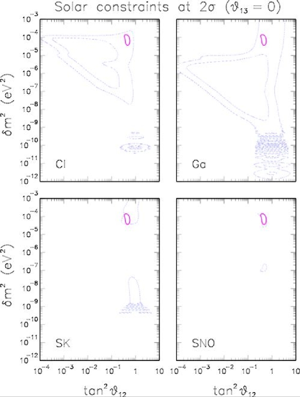
Figure 1: Regions separately allowed by the Chlorine (Cl), Gallium (Ga), Super-Kamiokande (SK) and Sudbury Neutrino Observatory (SNO) experiments at the $2\sigma$ level ($\Delta\chi^{2}=4$) in the $(\delta m^{2},\tan^{2}\theta_{12})$ plane, for $\theta_{13}=0$. The LMA region allowed at $2\sigma$ by the Cl+Ga+SK+SNO combination is superposed in each panel.

Figure 1 shows the current solar neutrino constraints from separate data sets (Chlorine, Gallium, SK, SNO) at the $2\sigma$ level, using the BS05 (OP) SSM input [100]. In each panel, we also superpose the small region allowed at $2\sigma$ around $\delta m^{2}\sim\mathrm{few}\times 10^{-5}$ eV² and $\tan^{2}\theta_{12}\sim\mathrm{few}\times 10^{-1}$, which provides the solution to the solar neutrino problem [14] at large mixing angle (LMA). In Fig. 1 one can appreciate that the global LMA solution completely overlaps with each of the regions separately allowed by the different experimental data (at $2\sigma$), i.e., there is a strong consistency between different observations. The shape of the global solar LMA solution appears to be dominated by SNO and (to a lesser extent) by the SK experiment. Since both SK and SNO are sensitive to the high-energy tail of the solar neutrino spectrum (i.e., to the ⁸B neutrino flux [100]), and since the SNO determination of the ⁸B flux is already a factor of two more accurate than the corresponding prediction in the BS05 (OP) standard solar model (see next Sec. 3.2), the shape of the global LMA solution in Fig. 1 is rather robust with respect to possible variations in the standard solar model input (including those related to the recent chemical controversy about the solar photospheric metallicity [98, 99, 100]).

Notice that current solar neutrino data, by themselves, identify a unique (LMA) solution in Fig. 1; this was not the case only a few years ago (see, e.g., [101, 102]), when at least another region at low $\delta m^{2}$ (“LOW” solution) was allowed [94]. From a test of hypothesis, we get that the current probability of the LOW solution is only $P_{\mathrm{LOW}}=1.2\times 10^{-3}$. Former solutions in the vacuum oscillation regime (VAC) or at small mixing angle (SMA) (with acronyms taken, e.g., from [101, 102]) are now characterized by exceedingly low probabilities ($P_{\mathrm{VAC}}=4.8\times 10^{-6}$ and $P_{\mathrm{SMA}}=4.0\times 10^{-8}$ from current solar neutrino data).

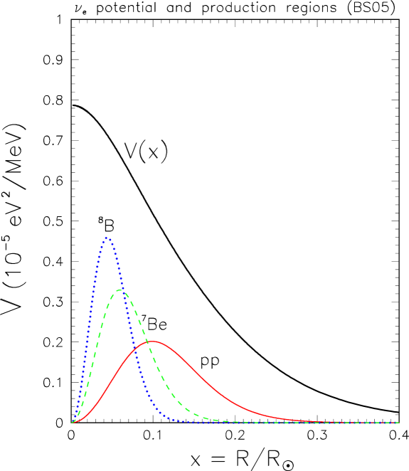
Figure 2: Neutrino potential $V=\sqrt{2}\,G_{F}N_{e}$ as a function of the normalized radius in the Sun. Also shown are the radial production regions for ⁸B, ⁷Be, and pp solar neutrinos (in arbitrary vertical scale). The curves refer to the Bahcall-Serenelli 2005 standard solar model.

The LMA solution is heavily affected by solar matter (MSW) effects (see, e.g., [103, 104] for a recent review of the LMA-MSW properties). Figure 2 shows the neutrino potential $V(x)$ as a function of the normalized Sun radius $x=R/R_{\odot}$, together with typical solar $\nu_{e}$ production regions (in arbitrary vertical scale), as taken from the BS05 (OP) model [99, 100]. From this figure one can easily derive that, for $\delta m^{2}$ values in the LMA region, matter effects are definitely important ($\delta m^{2}\sim A(x)$) for neutrinos with $E\sim\mathrm{few}$ MeV. More precisely, the LMA solar $\nu_{e}$ survival probability at the Earth [$P_{ee}=P(\nu_{e}\to\nu_{e})$] reads [4, 103]

$$P_{ee}=\frac{1}{2}+\frac{1}{2}\cos 2\tilde{\theta}_{12}(x)\cos 2\theta_{12}\ ,$$ (23)

where

$$\cos 2\tilde{\theta}_{12}=\frac{\cos 2\theta_{12}-A(x)/\delta m^{2}}{\sqrt{(\cos 2\theta_{12}-A(x)/\delta m^{2})^{2}+\sin^{2}2\theta_{12}}}\ ,$$ (24)

with $\cos 2\tilde{\theta}_{12}$ slowly changing from its vacuum value $(\cos 2\theta_{12})$ to its matter-dominated values (close to $-1$) as $E$ increases from sub-MeV to multi-MeV values.

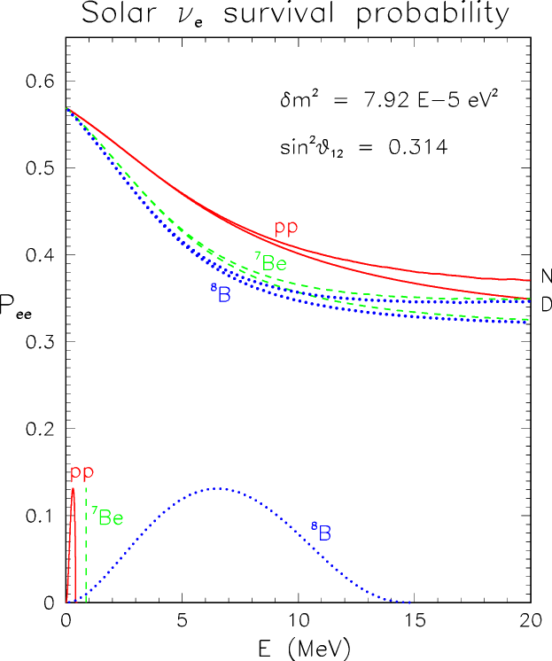
Figure 3: The energy profile of the solar $\nu_{e}$ survival probability $P_{ee}$ for best-fit LMA values and $\theta_{13}=0$. The function $P_{ee}(E)$ shows a smooth transition from vacuum to matter-dominated regime as $E$ increases, with some differences induced by averaging over different production regions (for ⁸B, ⁷Be and pp neutrinos) and, to a smaller extent, by nighttime (N) Earth effects with respect to daytime (D). Also shown are the corresponding solar neutrino energy spectra (in arbitrary vertical scale).

Figure 3 shows the energy profile of $P_{ee}$, averaged over the production regions relevant to pp, ⁷Be, and ⁸B solar neutrinos, for representative LMA oscillation parameters. Also shown are the energy profiles of corresponding solar $\nu_{e}$ fluxes (in arbitrary vertical scale). The value of $P_{ee}$ decreases from its vacuum value ($1-0.5\sin^{2}2\theta_{12}$) to its matter-dominated value $(\sim\sin^{2}\theta_{12})$ as the energy increases. The vacuum-matter transition is faster for neutrinos produced in the inner regions of the Sun. In Fig. 3 we also show the small difference between day (D) and night (N) curves, due to matter effects in the Earth (calculated, for definiteness, at the SNO latitude). The vacuum-matter transition is slightly slower during the night, due to the Earth regeneration effect (see [106] and references therein). Within current energy thresholds and experimental uncertainties, the vacuum-matter transition and the Earth regeneration effects have not been yet observed in the SK [14] and SNO [17] time-energy spectra. Nevertheless, as we shall see later, matter effects in the Sun must definitely occur to explain the data.

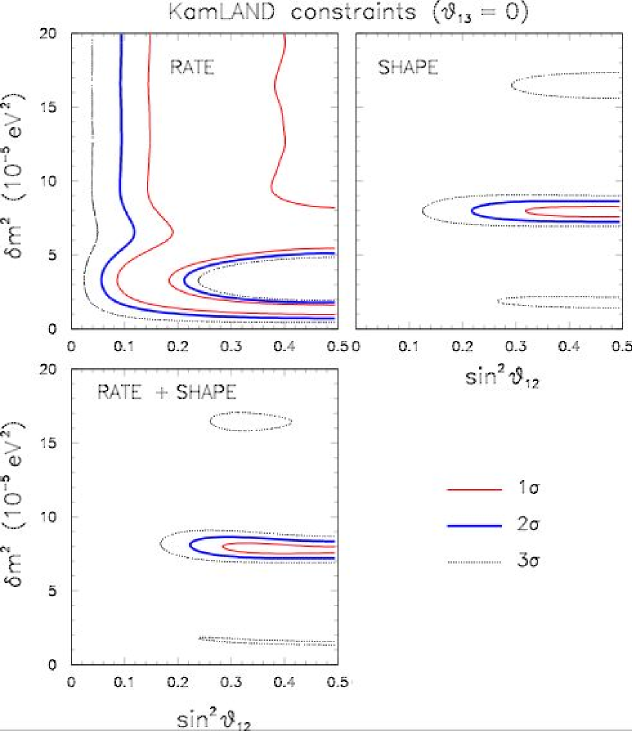
Figure 4: KamLAND constraints in the mass-mixing plane $(\delta m^{2},\sin^{2}\theta_{12})$ and for $\theta_{13}=0$, as derived by an unbinned maximum-likelihood analysis of the total rate, spectrum shape, and rate+shape information. Contours are shown at 1, 2, and $3\sigma$ level.

Let us consider now the impact of KamLAND data. For typical LMA parameters, reactor $\bar{\nu}_{e}$ are expected to have a relatively large oscillation amplitude ($\sin^{2}2\theta_{12}$), as well as a sizable oscillation phase [$\delta m^{2}L/4E\sim O(1)$] over long baselines ($L\sim O(10^{2})\mathrm{\ km}$). The $\bar{\nu}_{e}$ disappearance signal observed in KamLAND [19, 20] has not only confirmed the solar LMA solution but has greatly reduced its $\delta m^{2}$ range [20, 17], by observing a strong distortion in the energy spectrum [20]. Figure 4 shows the mass-mixing parameter regions separately allowed by the KamLAND total rate, by the energy spectrum shape, and by their combination, at the 1, 2, and $3\sigma$ level, as obtained by our unbinned maximum-likelihood analysis [93] of the latest energy spectrum data [21]. The overall reactor neutrino disappearance (rate information) and its energy distribution (shape information) are highly consistent, the latter being dominant in the combination. At the $2\sigma$ level, both the shape-only and the rate+shape analyses identify a single solution at $\delta m^{2}\sim 8\times 10^{-5}$ eV² and large mixing; only at the $3\sigma$ level two disconnected solutions appear at higher and lower values of $\delta m^{2}$. Notice the linear scale on both axes, and the reduction of the parameter space, as compared with Fig. 1.

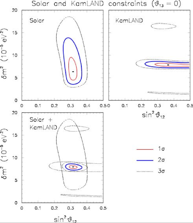
Figure 5: Solar and KamLAND constraints in the mass-mixing plane $(\delta m^{2},\sin^{2}\theta_{12})$ and for $\theta_{13}=0$, shown both separately and in combination, at 1, 2, and $3\sigma$ level.

Figure 5 shows the regions separately allowed by all solar neutrino data and by KamLAND, both separately and in combination, at the 1, 2, and 3$\sigma$ level. The current solar LMA solution, as compared with results prior to complete SNO-II data (see, e.g., [16, 20, 107], is slightly shifted toward larger values of $\sin^{2}\theta_{12}$ and allows higher values of $\delta m^{2}$. This trend is substantially due to the larger value of the CC/NC ratio measured in the complete SNO II phase (0.34 [17]) with respect to the previous central value (0.31 [16]). We also find that the SNO-II CC spectral data [17] contribute to allow slightly higher values of $\delta m^{2}$ with respect to older results. The consistency of solar and reactor allowed regions is impressive, with a large overlap even at the $1\sigma$ level, and with very close best-fit points. The solar+KamLAND combination eliminates the extra (KamLAND-only) solutions at high and low $\delta m^{2}$, and identifies a single allowed region characterized by the following $2\sigma$ ranges:

$$\delta m^{2}=7.92\times 10^{-5}\mathrm{\ eV}^{2}\,(1\pm 0.09)\ \mathrm{\ at\ }\pm 2\sigma\ ,$$ (25)

$$\sin^{2}\theta_{12}=0.314\,(1^{+0.18}_{-0.15})\ \mathrm{\ at\ }\pm 2\sigma\ .$$ (26)

The determination of these two parameters at $O(10\%)$ level represents one of the most remarkable successes of the last few years in neutrino physics.

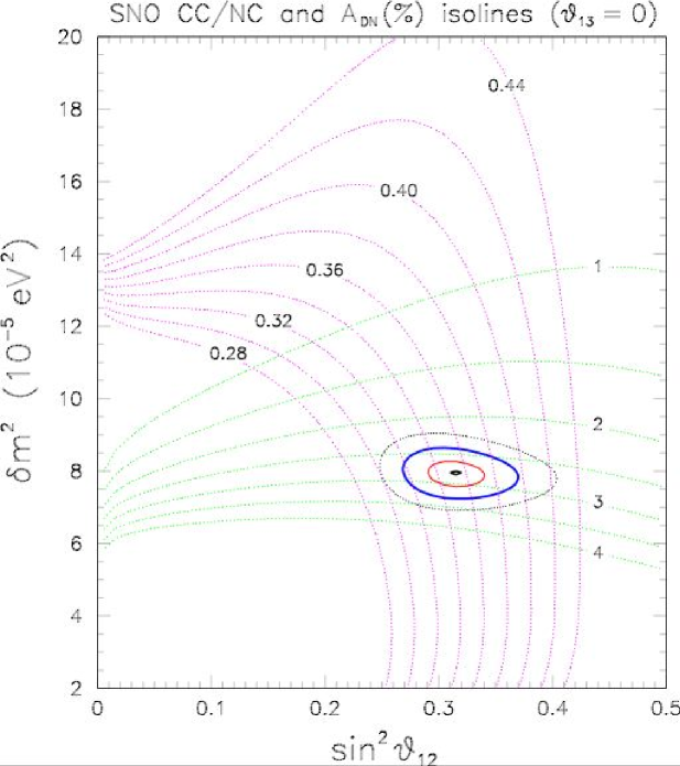
Figure 6: Isolines of the charged-to-neutral current flux ratio and of the day-night asymmetry in SNO, superposed to the global (solar+KamLAND) LMA allowed region.

The $\delta m^{2}$ uncertainty is currently dominated by the KamLAND observation of half-period of oscillations [20] and can be improved with higher statistics [108]. The $\sin^{2}\theta_{12}$ uncertainty is instead dominated by the SNO ratio of CC to NC events, which is a direct measurement of $P_{ee}$ at high energy: $R_{\mathrm{CC}}/R_{\mathrm{NC}}\simeq P_{ee}\simeq\sin^{2}\theta_{12}$. Figure 6 shows isolines of this ratio in the mass-mixing parameter space, which can be used as a guidance [109, 110] to understand the effect of prospective SNO measurements on the $\sin^{2}\theta_{12}$ range. In the same figure we show isolines of the day-night asymmetry ($A_{\mathrm{DN}}$) of CC events in SNO, whose measurement could, in principle, help to reduce the $\delta m^{2}$ uncertainty [109, 110]; however, it is unlikely that the SNO errors can be reduced enough ($<1\%$) to clearly observe a day-night effect (see, e.g., [111]).

3.2 Evidence for matter effects in the Sun

As shown in Fig. 3, solar matter effects make $P_{ee}$ decrease from its vacuum value ($>1/2$) to a matter-dominated value ($<1/2$), for typical LMA parameters around the current best fit. Model-independent tests of the presence of matter effects are derived in the following, first by showing that SK and SNO data consistently indicate that $P_{ee}<1/2$ in their energy range, and secondly by showing that all solar+reactor data consistently indicate that the neutrino potential $V(x)$ must be nonzero.

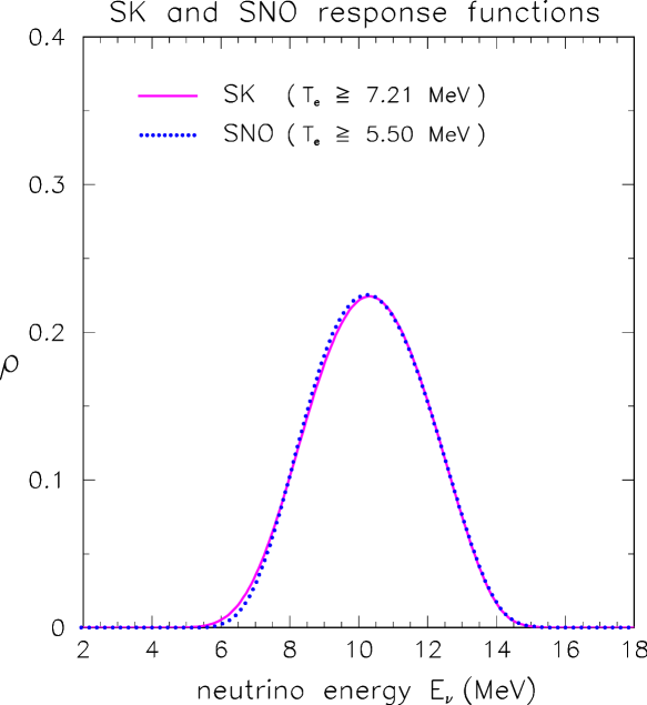
Figure 7: SNO response function for electron kinetic energy threshold $T_{e}\geq 5.5$ MeV, and equalized SK response function at $T_{e}\geq 7.21$ MeV. For such threshold, the SNO (CC) and SK (ES) solar $\nu$ measurements are sensitive to the same parent neutrino energy spectrum, up to the negligible differences between the two curves in the figure.

As discussed in [112, 113], the normalized energy spectra of neutrinos which do interact in SK and in SNO (i.e., the SK and SNO “response functions” to the incoming ⁸B neutrinos) can be equalized, to a good approximation, by choosing a proper SK energy threshold, for any given SNO threshold. The current best “equalization” of SK and SNO response functions is shown in Fig. 7. In this case, both SK and SNO are sensitive to the same energy-averaged survival probability, $\langle P_{ee}\rangle$. Moreover, the CC and NC event rates in SNO, together with the ES event rate in SK, overconstrain $\langle P_{ee}\rangle$ and the unoscillated ⁸B solar neutrino flux $\Phi_{B}$ in a completely model-independent way (i.e., independently of the mass-mixing parameters and of the standard solar model) through the equations [112, 113]

$$\Phi_{\mathrm{ES}}^{\mathrm{SK}} = \Phi_{B}[\langle P_{ee}\rangle+r_{\sigma}(1-\langle P_{ee}\rangle)]\ ,$$ (27)

$$\Phi_{\mathrm{CC}}^{\mathrm{SNO}} = \Phi_{B}\langle P_{ee}\rangle\ ,$$ (28)

$$\Phi_{\mathrm{NC}}^{\mathrm{SNO}} = \Phi_{B}\ ,$$ (29)

where $r_{\sigma}\simeq 0.154$ is the ratio of the energy-averaged ES cross-sections of $\nu_{\mu,\tau}$ and $\nu_{e}$ in SK.

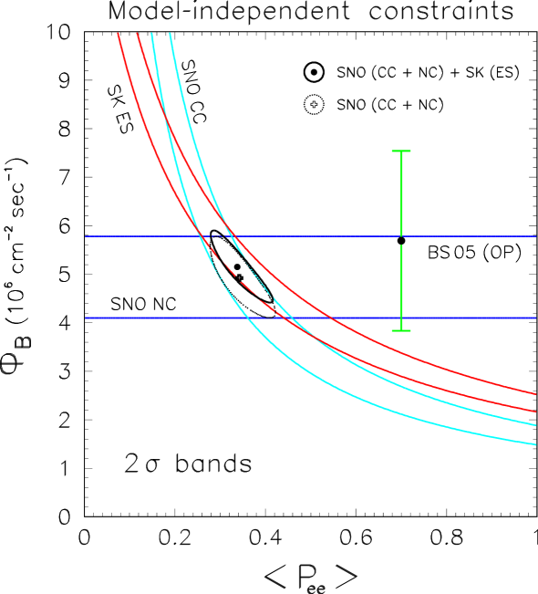
Figure 8: Model-independent SK+SNO constraints on the flux $\Phi_{B}$ of solar ⁸B neutrinos and on their survival probability $P_{ee}$ (at $2\sigma$), averaged over the common response function in Fig. 7. Also shown is the $\pm 2\sigma$ range of $\Phi_{B}$ from the BS05 (OP) standard solar model.

Figure 8 shows the current bounds at $2\sigma$ on $\Phi_{B}$ and $\langle P_{ee}\rangle$, as obtained by using the latest SNO CC and NC [17] and SK ES [13, 14] event rates, both separately (bands) and in combination ($2\sigma$ elliptical regions). The dotted ellipse represent the combination of SNO NC and CC data; the addition of SK ES data—which are consistent with SNO NC and CC data—slightly increases the preferred value of $\Phi_{B}$ (solid ellipse). In particular, the SNO+SK combination (dominated by SNO) provides the following ranges:

$$\Phi_{B}=5.2^{+0.7}_{-0.8}\times 10^{6}\mathrm{cm}^{-2}\mathrm{s}^{-1}\ \ (\pm 2\sigma)\ ,$$ (30)

$$\langle P_{ee}\rangle=0.34^{+0.08}_{-0.06}\ \ (\pm 2\sigma)\ .$$ (31)

The above SNO+SK range for $\Phi_{B}$ is consistent with the $\pm 2\sigma$ prediction of the BS05(OP) standard solar model [100], $\Phi_{B}^{\mathrm{SSM}}=5.7(1\pm 0.32)\times 10^{6}\mathrm{cm}^{-2}\mathrm{s}^{-1}$, the difference in the central values ($\sim 10\%$) being not statistically significant, as also evident in Fig. 8. Notice that the SK+SNO data determine $\Phi_{B}$ with an error a factor of 2 smaller than the SSM prediction. At the same time, the SK+SNO data constrain $\langle P_{ee}\rangle$ to be definitely less than $1/2$ [114, 115], and in particular close to $\sim 1/3$, as predicted for high-energy ⁸B neutrinos and LMA parameters (see Fig. 3). The model-independent SNO+SK analysis is thus fully consistent with the LMA-MSW expectations; removal of the MSW effect in the LMA region would give a prediction $\langle P_{ee}\rangle=1-0.5\sin^{2}2\theta_{12}>1/2$, inconsistently with the results in Fig. 8.

One can perform, however, a more powerful test of the presence of the neutrino potential $V(x)$, by artificially altering its magnitude through a free parameter $a_{\mathrm{MSW}}$ [114, 115, 116],

$$V(x)\to a_{\mathrm{MSW}}\,V(x)\ ,$$ (32)

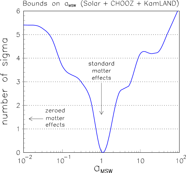
Figure 9: Bounds on the amplitude of matter effects, taken as a free parameter $a_{\mathrm{MSW}}$. The cases $a_{\mathrm{MSW}}=1$ and $a_{\mathrm{MSW}}=0$ correspond to standard and no matter effects, respectively. The vertical axis represents the number of standard deviations (i.e., $\sqrt{\Delta\chi^{2}}$) from the best-fit, as obtained by an analysis of all solar and reactor (KamLAND+CHOOZ) data with marginalized $(\delta m^{2},\sin^{2}\theta_{2})$ parameters. Standard matter effects are confirmed within a factor of $\sim 2$ uncertainty at $2\sigma$.

both in the Sun (relevant for solar neutrino oscillations) and in the Earth (relevant for both solar and reactor neutrino oscillations), and by renalyzing solar and KamLAND data with $a_{\mathrm{MSW}}$ free. Testing matter effects amounts then to reject the case $a_{\mathrm{MSW}}=0$ (no effect) and to prove that $a_{\mathrm{MSW}}=1$ (standard effect) is favored. In the analysis, we add CHOOZ reactor data, which help to exclude the appearance of spurious high-$\delta m^{2}$ solutions for $a_{\mathrm{MSW}}\gg 1$ [114, 115, 116]. Figure 9 shows the results of a fit to all the current solar and reactor data in the parameter space $(\delta m^{2},\sin^{2}\theta_{12},a_{\mathrm{MSW}})$, marginalized with respect to the first two parameters, in terms of the function $(\Delta\chi^{2})^{1/2}=n\sigma$. The preference for standard matter effects $(a_{\mathrm{MSW}}=1)$ is really impressive, and is currently even more pronounced then with previous data [116]. The hypothetical case of no matter effects $(a_{\mathrm{MSW}}=0)$ is rejected at $>5\sigma$. Since $V\propto G_{F}$, the results in Fig. 9 can not only be seen as a confirmation of matter effects, but can also be interpreted as an alternative “measurement” of the Fermi constant $G_{F}$ through neutrino oscillations in matter, within a factor of $\sim 2$ uncertainty at $2\sigma$.

3.3 Statistical checks

We have seen that, globally, solar neutrino experiments agree with each other and with the KamLAND observation of reactor neutrino disappearance, that solar+KamLAND data identify a restricted range of LMA mass-mixing parameters, and that there is solid evidence for the associated matter effects in such range. However, it makes sense to look at the statistical consistency of the LMA best-fit solution in more detail, for at least two reasons: (1) the analysis involves a large number of observables and of systematics, some of which might deviate from the predictions without really altering the global fit; (2) the preferred shifts of some quantities might reveal something interesting.

We remind that the solar neutrino analysis is performed through the so-called pull approach [94], namely, by allowing shifts of each $n$-th theoretical prediction $R_{n}$ through independent systematic uncertainties $c_{nk}$,

$$R_{n}\to\overline{R}_{n}=R_{n}+\sum_{k}\xi_{k}\,c_{nk}\ ,$$ (33)

whose amplitudes $\xi_{k}$ are constrained through a quadratic penalty term. The shifted predictions $\overline{R}_{n}$’s are then compared to the experimental values $R_{n}^{\mathrm{exp}}$ via the uncorrelated (mainly statistical) error components. The method can be generalized to include correlation of statistical [95] and systematic [117] errors. The global $\chi^{2}$ function is then given by two terms, $\chi^{2}=\chi^{2}_{\mathrm{obs}}$ + $\chi^{2}_{\mathrm{sys}}$, embedding the quadratic pulls of the observables (i.e., the deviations of theory vs experiment) and of the systematics (i.e., their offset with respect to zero). This method allow a detailed check of possible pathological deviations (pulls) of some quantities. (See also the Appendix.)

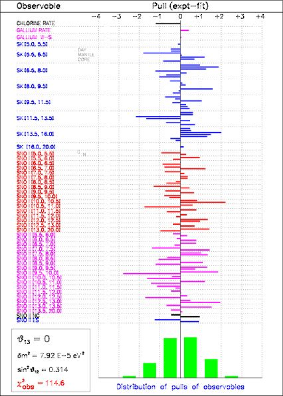
Figure 10: Pulls (at the global best-fit point for $\theta_{13}=0$) of all the observables included in the solar neutrino data analysis.

Figure 10 shows the pulls of the 119 observables at the global (solar+KamLAND) best-fit point. From top to bottom, the observables include the Chlorine rate, the Gallium rate and its winter-summer asymmetry [118, 12], the SK distribution in energy and zenith angle (44 bins) [13, 14], the SNO-I (no-salt) CC spectrum in 17+17 day-night bins [15], the SNO-II (with salt added) CC spectrum in 17+17 day-night bins and the day-night values of the NC and ES rate [17]. The SNO-II data and their correlations are treated as prescribed in [17]; for all the other observables we refer the reader to [94]. None of the pulls in Fig. 10 exceeds $3\sigma$, and their distribution, which is roughly gaussian, reveals nothing pathological. We conclude that none of the solar neutrino observables shows an anomalous or suspect deviation from the LMA best-fit predictions.

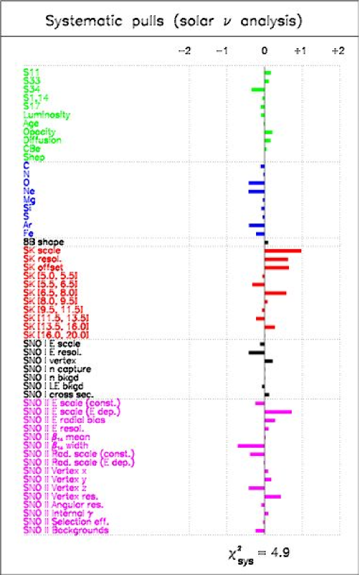
Figure 11: Pulls (at the global best-fit point) of the systematics included in the solar neutrino data analysis.

Figure 11 shows the pulls of the 55 systematic errors which enter in the analysis. From top to bottom, they include 11 “old” standard solar systematics as in [94], 9 “new” SSM metallicity systematics [98], the ⁸B spectrum shape uncertainty [119], 11 SK and 7 SNO-I systematics as in [94], and 16 “new” SNO-II systematics [17]. All the offsets are small $(<1\sigma)$, indicating that the allowance to shift the theoretical predictions $R_{n}$ through systematic uncertainties is only moderately exploited in the fit; in other words, there is no need to stretch the systematics beyond their stated $1\sigma$ range to achieve a good fit.

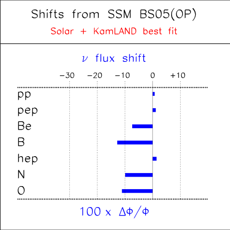
Figure 12: Preferred shifts of the solar neutrino fluxes (at the global best-fit point) with respect to the central values of the BS 2005 (OP) standard solar model.

Finally, Fig. 12 shows a by-product of the pull approach, namely, the preferred shifts of the solar neutrino fluxes with respect to their central SSM values [94]. The $\sim 10\%$ downward shift of $\Phi_{B}$ is consistent with the results in Fig. 8. The global fit also prefers a $\sim 10\%$ reduction of beryllium (Be) and CNO solar neutrino fluxes with respect to the BS05 (OP) prediction—an indication which may be of interest for future experiments directly sensitive to such fluxes [120, 121]. Such preferred reductions are well within SSM uncertainties [100].

In conclusion, the detailed analysis of the LMA best-fit solution reveals a very good agreement between all single pieces of experimental and theoretical information in the solar neutrino analysis. No statistically alarming deviation is found.

Concerning the statistical analysis of KamLAND data, the adopted maximum-likelihood approach [93] involves only three systematic uncertainties, namely, two free background normalization factors $\alpha^{\prime}$ and $\alpha^{\prime\prime}$ plus one constrained pull $\alpha$ for the energy scale offset (the overall rate normalization error being incorporated in the likelihood rate factor, see the Appendix and [93]). Therefore, our pull analysis for KamLAND involves a single parameter ($\alpha$), which we find to be very small ($\alpha\simeq 0.15\sigma_{\alpha}$) at the LMA best fit. In addition, as discussed in [93], the statistical analysis of KamLAND data shows no hints for anomalous effects beyond the standard scenario involving known reactor sources and neutrino flavor disappearance.

3.4 Solar and KamLAND constraints ($\theta_{13}$ free)

For $\theta_{13}>0$, electron neutrino mixing includes also $\nu_{3}$ (besides $\nu_{1}$ and $\nu_{2}$), and $\Delta m^{2}$-driven oscillations can take place, with amplitude governed by $\theta_{13}$. Therefore, the $\nu_{e}$ survival probability for $\theta_{13}>0$ ($P_{3\nu}$) generally differs from the one for $\theta_{13}=0$ ($P_{2\nu}$).

In KamLAND, $\Delta m^{2}$-driven oscillations are so fast to be smeared away by the finite energy resolution, leaving only the average ($\theta_{13}$ mixing) effect,

$$P_{3\nu}=c^{4}_{13}P_{2\nu}+s^{4}_{13}\ .$$ (34)

In first approximation, a similar formula holds for solar neutrinos, provided that the neutrino potential $V$ is multiplied everywhere by $\cos^{2}\theta_{13}$ (see [81, 122] and refs. therein):

$$P_{3\nu}\simeq c^{4}_{13}P_{2\nu}^{\prime}+s^{4}_{13}\ ,$$ (35)

$$P_{2\nu}\to P_{2\nu}^{\prime}=P_{2\nu}\big{|}_{V\to c^{2}_{13}V}\ .$$ (36)

This replacement generates a mild energy-dependence of the correction, which is absent in Eq. (34).

In second approximation, solar neutrinos develop a subleading dependence of $P_{3\nu}$ on $\Delta m^{2}$ [63] and on its sign (i.e., on the hierarchy, see [85]; such dependence disappears for $\Delta m^{2}\to\infty$, where one recovers the above equations. Accurate analytic expressions for the subleading $\Delta m^{2}$ effects on $P_{3\nu}$ as a function of energy can be found in [85].

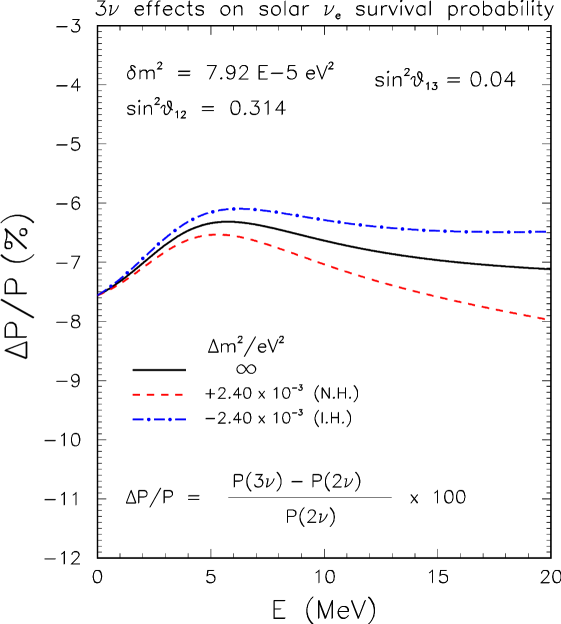
Figure 13: Representative estimate of leading and subleading effects which modify the solar neutrino survival probability from $P_{2\nu}$ ($\theta_{13}=0$) to $P_{3\nu}$ ($\theta_{13}>0$). See the text for details.

Figure 13 shows the size of leading ($\theta_{13}$-driven) and subleading ($\pm\Delta m^{2}$-driven) effects, through the fractional difference between $P_{2\nu}$ and $P_{3\nu}$, calculated for the representative value $s^{2}_{13}=0.04$ and for best-fit LMA parameters (and averaged over the ⁸B solar neutrino production region, for definiteness). The solid curve is calculated for $\Delta m^{2}=\infty$, i.e., no subleading effect; the leading effect (about $-7\%$) is almost entirely due to the factor $c^{4}_{13}$ in front of $P_{2\nu}$, plus a mild energy dependence. The dashed and dot-dashed curves are instead calculated for $\Delta m^{2}=+2.4$ and $-2.4$ ($\times 10^{-3}$ eV²), respectively; their difference from the solid curve quantifies the size of $\Delta m^{2}$ subleading effects. Although the dependence of $P_{3\nu}$ on $\Delta m^{2}$ and on the hierarchy is theoretically interesting (see, e.g., [122]), such subleading effect is an order of magnitude smaller than the “leading” $\theta_{13}$-effect in Fig. 13, and its inclusion would not change in any appreciable way the analysis of solar neutrino data (as we have explicitly checked). Therefore, in the following, we can safely assume the approximations in Eqs. (35) and (36), i.e., neglect the effect of $\Delta m^{2}$ and its sign in the solar(+KamLAND) data analysis, as it was the case for older data [123].

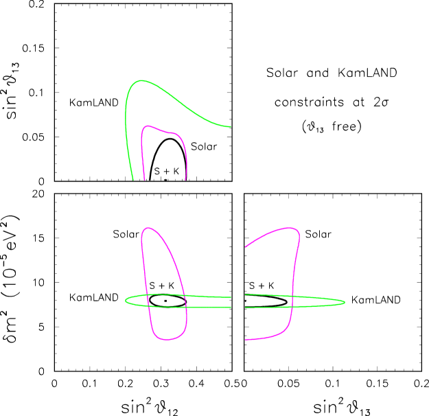
Figure 14: Three flavor analysis of solar and KamLAND data (both separately and in combination) in the parameter space $(\delta m^{2},\sin^{2}\theta_{12},\sin^{2}\theta_{13})$. The contours represent projections of the region allowed at $2\sigma$ ($\Delta\chi^{2}=4$).

Figure 14 shows the results of our analysis of solar and KamLAND data (both separately and in combination) for unconstrained values of $\theta_{13}$, in terms of the $2\sigma$ projections of the $(\delta m^{2},\sin^{2}\theta_{12},\sin^{2}\theta_{13})$ allowed region onto each of the three coordinate planes. There is no statistically significant preference for $\theta_{13}\neq 0$, and upper bounds are placed by both solar and KamLAND data separately.

Concerning KamLAND data only, there is a slight anticorrelation between $\sin^{2}\theta_{13}$ and $\sin^{2}\theta_{12}$ (upper left panel in Fig. 14), since the total rate information constrains both parameters [124], and a higher $\sin^{2}\theta_{13}$ can be traded for a lower $\sin^{2}\theta_{12}$. However, $\sin^{2}\theta_{12}$ cannot decrease indefinitely—since it would suppress the amplitude of the observed shape distortions [20]—and thus an upper bound on $\sin^{2}\theta_{13}$ emerges in KamLAND.

We remind that the solar $\nu$ sensitivity to $\sin^{2}\theta_{13}$ (Fig. 14) comes from the combination of all solar neutrino experiments, in contrast with the bounds on $(\delta m^{2},\sin^{2}\theta_{12})$, which are dominated by the “high energy” ⁸B neutrino experiments (SNO and SK). As discussed, e.g., in [122], for increasing values of $\theta_{13}$ a tension arises among different data sets and, in particular, between SNO and Gallium data. Such two experiments, probing respectively the high and low energy part of the solar neutrino spectrum, exhibit different correlation properties between the two mixing parameters $\theta_{12}$ and $\theta_{13}$. In particular, for increasing values of $\theta_{13}$, the SNO and Gallium experiments tend to prefer higher and lower values of $\sin^{2}\theta_{12}$, respectively [122], worsening the good agreement currently reached at $\theta_{13}\simeq 0$. Therefore, a “collective” effect of different experiments is responsible for the solar neutrino constraints on $\sin^{2}\theta_{13}$. (See also [50] for a discussion of bounds on $\theta_{13}$ with earlier data.)

Very interestingly, the combination of solar and KamLAND data in Fig. 14 is now powerful enough to place a combined upper bound on $\sin^{2}\theta_{13}$ at the 5% level at $2\sigma$, not much weaker than the bound coming from the CHOOZ plus atmospheric data discussed below in Sec. 4.3 (see also [125] for an earlier discussion of solar+KamLAND constraints on $\theta_{13}$). Notice also that, in the combined (solar+KamLAND) regions of Fig. 14, there are negligible correlations among the three parameters; this fact implies that the bounds in Eqs. (25) and (26), derived for $\theta_{13}=0$, hold without significant changes also for $\theta_{13}$ unconstrained. It also justifies (a posteriori) our choice to discuss in detail the case $\theta_{13}=0$, which embeds most of the relevant information on the leading parameters $(\delta m^{2},\sin^{2}\theta_{12})$.

4 SK atmospheric neutrinos, K2K, and CHOOZ

In this Section we discuss the constraints on the mass-mixing parameters $(\Delta m^{2},\theta_{23},\theta_{13})$ coming from the SK atmospheric neutrino detector [26], from the K2K long-baseline accelerator neutrino experiment [30, 31], and from the short-baseline CHOOZ reactor neutrino experiment [32].

Our SK atmospheric neutrino analysis is performed by using the same event classification (binning) and systematic error treatment as in [117]. In particular, we consider (in order of increasing average energy) the zenith angle distributions of the so-called Sub-GeV (SG) electron and muon samples (SG$e$ and SG$\mu$) in 10 zenith angle $(\theta_{z})$ bins; Multi-GeV (MG) electron and muon samples (MG$e$ and MG$\mu$) in 10 zenith angle $(\theta_{z})$ bins; Upward Stopping muons (US$\mu$) in 5 bins; and Upward Through-going muons (UT$\mu$) in 10 bins, for a total of 55 accurately computed observables. We include 11 sources of systematic errors [117] with the pull method [94] which allows a better understanding of systematic shifts. With respect to our previous SK analysis [117], we use updated results [26] and—unless otherwise stated—atmospheric neutrino input fluxes from the three-dimensional (3D) simulation of [126] (see also [127, 128] for other 3D results).

Concerning the K2K experiment, we use the latest spectrum data from [31], but regrouped in the same 6 bins as in [117] (by using information from [129]); this choice is motivated by the fact that information about K2K correlated systematics has been made publicly available only for 6 bins (see [117] and references therein). Finally, the CHOOZ spectral data [32] are analyzed as in [85]. Further technical details are given in the Appendix.

In the following, we discuss first the impact of the SK+K2K data on the neutrino parameters $(\Delta m^{2},\sin^{2}\theta_{23})$ for $\theta_{13}=0$. This allows to appreciate the subleading effect induced by nonzero values of $(\delta m^{2},\sin^{2}\theta_{12})$, especially on atmospheric neutrinos. Then we consider the more general case $\theta_{13}\neq 0$, and discuss in some detail the related subleading effects in SK, as well as the constraints from the SK+K2K+CHOOZ analysis.

A final remark is in order. The MACRO [27] and Soudan-2 [28] atmospheric neutrino experiments provide $(\Delta m^{2},\sin^{2}\theta_{23})$ constraints which are consistent with those from SK [26], but are also affected by larger uncertainties (due to the lower statistics and narrower $L/E$ range); they are not included in this work. Similarly, the negative results of the Palo Verde reactor experiment [33] and of the K2K searches in $\nu_{\mu}\to\nu_{e}$ appearance mode [130] (consistent with, but less constraining than CHOOZ [32]) are not included here. Future improved global analyses might take into account these additional data, finer SK and K2K spectral binning, and the covariance of the SK and K2K common systematics (interaction cross section, detector fiducial volume, and event reconstruction errors).

4.1 SK and K2K constraints for $\theta_{13}=0$ and statistical checks

While for $\theta_{13}=0$ the solar+KamLAND parameter space reduces to $(\delta m^{2},\sin^{2}\theta_{12})$ exactly, the atmospheric+K2K parameter space reduces to $(\Delta m^{2},\sin^{2}\theta_{23})$ only to a first approximation. Indeed, while the assumption $\theta_{13}=0$ forbids solar and reactor $\nu_{e}\to\nu_{\mu,\tau}$ transitions involving $\nu_{3}$ and its associated parameters ($\Delta m^{2},\sin^{2}\theta_{23}$), it does not forbid, e.g., atmospheric $\nu_{\mu}\to\nu_{\tau}$ transitions involving the pair $(\nu_{1},\nu_{2})$, which depend on the $\delta m^{2}$ parameter. This is most easily seen in the vacuum case, where Eq. (20) implies that, for $i,j=1,2$ and even for $\theta_{13}=0$, the $P_{\mu\tau}$ transition probability contains the following nonzero $(\nu_{1},\nu_{2})$-induced term,

$$-4U_{\mu 1}U_{\mu 2}U_{\tau 1}U_{\tau 2}\sin^{2}\left(\frac{m^{2}_{2}-m^{2}_{1}}{4E}\,L\right)\stackrel{{\scriptstyle\theta_{13}=0}}{{=}}-4s^{2}_{12}c^{2}_{12}s^{2}_{23}c^{2}_{23}\sin^{2}\left(\frac{\delta m^{2}}{4E}\,L\right)\ .$$ (37)

The small effect of nonzero (LMA) values of $(\delta m^{2},\sin^{2}\theta_{12})$ in the atmospheric neutrino data analysis, phenomenologically noted in [123] for any $\theta_{13}$, has often been legitimately neglected (except occasionally, see the bibliography in [131]), being basically hidden by large statistical and systematic uncertainties. The full implementation of such effect is nontrivial (it requires a numerical $3\nu$ evolution in the Earth matter layers), and its main theoretical aspects have been elucidated only recently [131, 132], in connection with the progressive confirmation and determination of the LMA parameters by solar and KamLAND data, and with the increasing accuracy of atmospheric neutrino data. Although still small, the effect is definitely not smaller than others which are usually taken care of, and deserves to be included in state-of-the-art analyses [132, 133, 134].

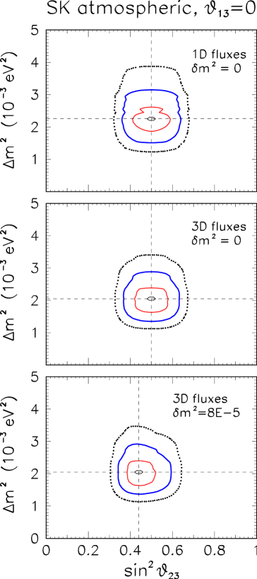
Figure 15: Analysis of SK atmospheric neutrino data in the plane $(\Delta m^{2},\sin^{2}\theta_{23})$ at $\theta_{13}=0$, for increasingly accurate inputs. The curves represent bounds at 1, 2 and $3\sigma$ level. Upper panel: one-dimensional input fluxes and $\delta m^{2}=0$. Middle panel: three-dimensional input fluxes and $\delta m^{2}=0$. Lower panel: three-dimensional input fluxes and $(\delta m^{2},\sin^{2}\theta_{12})$ fixed at their best-fit LMA values.

For instance, Fig. 15 shows the results of our analysis of the latest SK data in the plane $(\Delta m^{2},\sin^{2}\theta_{23})$ at $\theta_{13}=0$, for three increasingly accurate inputs: Atmospheric neutrino fluxes from one-dimensional (1D) simulations and $\delta m^{2}=0$ (top panel); atmospheric neutrino fluxes from full three-dimensional (3D) simulations [126] and $\delta m^{2}=0$ (middle panel); and finally, 3D fluxes and LMA best-fit values for $(\delta m^{2},\sin^{2}\theta_{12})$. In all panels, the three curves refers to 1, 2, and $3\sigma$ contours, and the best-fit point is marked by horizontal and vertical lines to guide the eye. One can appreciate that the (now customarily included) 3D flux input shifts $\Delta m^{2}$ downward by $\sim 0.5\sigma$ with respect to the 1D flux input; on the other hand, the inclusion of subleading LMA effects shifts $\sin^{2}\theta_{23}$ by $\sim 0.5\sigma$ [133] with respect to the hypothetical case $\delta m^{2}=0$. As expected, both effects are small, but there is no reason to keep the first and to neglect the second. Moreover, the LMA effect intriguingly breaks the $\theta_{23}$ octant sysmmetry, which is in principle an important indication for model building (see, e.g., [135]). Hereafter, the analysis of the SK atmospheric data will explicitly include nonzero values of $(\delta m^{2},\sin^{2}\theta_{12})$, fixed at their best-fit values in Eqs. (25, 26) but with no uncertainty (whose effect is really negligible). For the sake of completeness, LMA-induced and matter effects will also be included in the calculation of the K2K oscillation probabilities, where, however, such effects are even smaller than in SK, as discussed in Sec. 4.2.

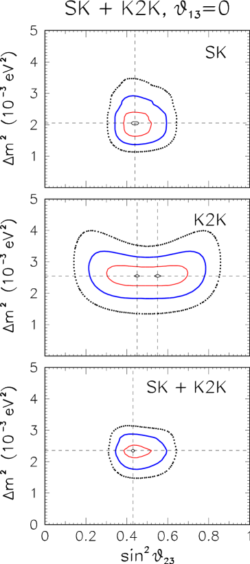
Figure 16: Analysis of SK and K2K data (both separately and in combination) in the plane $(\Delta m^{2},\sin^{2}\theta_{23})$ at $\theta_{13}=0$. The parameters $(\delta m^{2},\sin^{2}\theta_{12})$ have been fixed at their best-fit LMA values.

Figure 16 shows, for $\theta_{13}=0$, the results of our analysis of SK and K2K data, both separately and in combination. Notice that the top panel in Fig. 16 is the same as the bottom panel in Fig. 15. The K2K constraints are octant-symmetric and relatively weak in $\sin^{2}\theta_{23}$, while they contribute appreciably to reduce the overall $\Delta m^{2}$ uncertainty. Therefore, not only K2K confirms the neutrino oscillation solution to the atmospheric neutrino anomaly with accelerator neutrinos [31], but it also helps in reducing the oscillation parameter space. Moreover, there is still room for improvements in K2K. Figure 17 shows our both unoscillated and oscillated K2K spectrum of events (at the SK+K2K best-fit in Fig. 16) in terms of the reconstructed neutrino energy, as used in this work. The oscillated spectrum is shown both with and without the systematic shifts in our pull approach; such shifts are modest as compared with the large statistical errors. Therefore, one can reasonably expect that, with higher statistics, the final K2K data sample can further contribute to reduce the $\Delta m^{2}$ uncertainty.

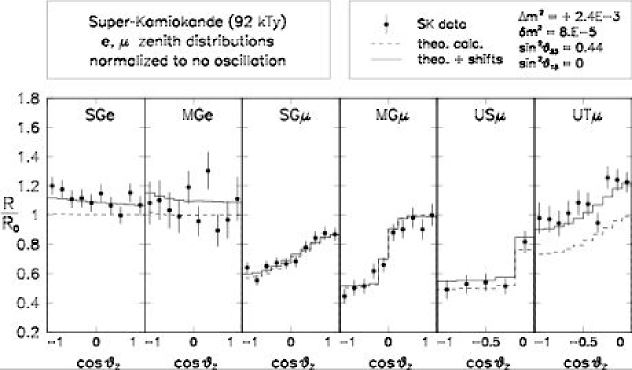
Figure 18: SK distributions of leptonic events as a function of the cosine of the lepton zenith angle $\theta_{Z}$, normalized to no-oscillation expectations in each bin. From left to right, the data samples refer to sub-GeV electrons (SG$e$), multi-GeV electrons (MG$e$), sub-GeV muons (SG$\mu$), multi-GeV muons (MG$\mu$), upward stopping muons (UP$\mu$), upward through-going muons (UT$\mu$). Data are shown by dots with $\pm 1\sigma$ statistical error bars. The histograms represent our calculations at the SK+K2K best fit in Fig. 16 (dashed: with no systematic shifts; solid: with systematic shifts allowed).

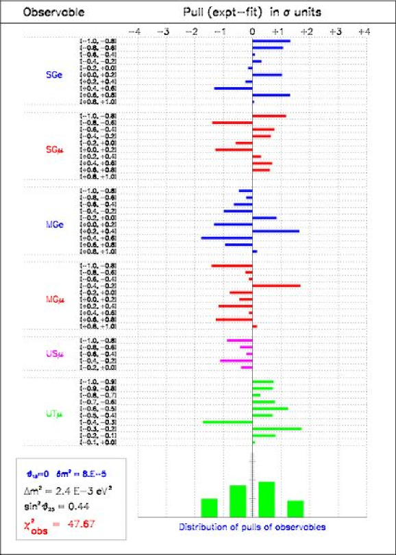
Figure 19: Pull analysis (bin-by-bin) of the SK observables in Fig. 18.

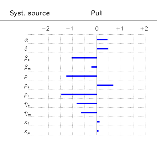
Figure 20: Pull analysis of the eleven systematic error sources included in the SK analysis. From top to bottom, systematic pulls refer to: overall normalization $(\alpha)$; energy spectrum slope $(\delta)$; $\mu/e$ flavor ratio for sub-GeV $(\beta_{s})$ and multi-GeV $(\beta_{m})$ events; relative normalization of partially and fully contained events $(\rho)$; normalization of all upgoing muon events $(\rho_{s})$ and of through-going muon events alone $(\rho_{t})$; up-down asymmetry error of sub-GeV $(\eta_{s})$ and multi-GeV $(\eta_{m})$ events; horizontal/vertical error of low-energy $(\kappa_{f})$ and high-energy $(\kappa_{\mu})$ events.

Systematic effects are instead quite important in the SK atmospheric neutrino analysis. Fig. 18 shows the ratio of experimental data [26] and of best-fit theoretical predictions (with and without systematic pulls) with respect to no oscillations, as a function of the zenith angle of the scattered lepton ($e$ or $\mu$), for the five samples used in the analysis. In particular, in terms of Eq. (33), the dashed histograms represent the unshifted theoretical predictions (central values $R_{n}$), while the dashed histograms represent the systematically shifted predictions ($\overline{R}_{n}$) for the given mass-mixing parameters (which correspond to the SK+K2K best-fit point in Fig. 16). Vertical error bars represent the $1\sigma$ statistical uncertainties of the data. The electron data (SG$e$ and MG$e$) show some excess with respect to the unshifted predictions (dashed lines), which tends to be reduced when systematic shifts are allowed (solid lines). Notice that the dashed lines slightly differ from unity for upward $(\cos\theta_{z}\sim-1)$ events in the SG$e$ and MG$e$ sample, as a result of subleading LMA effects ($\delta m^{2}\neq 0$). A systematic, upward shift of the predictions is also preferred in the high-energy muon samples, US$\mu$ and UT$\mu$, and especially in the latter, where it amounts to $\sim 20\%$. The pull analysis of the observables in Fig. 19 tells us that such shifts are not necessarily alarming from a statistical viewpoint, since they are all smaller than two standard deviations. However, their distribution is definitely not random: within each of the six data samples, most of the pulls in Fig. 19 are one-sided, indicating that there seems to be some normalization offset. This is confirmed by the pull analysis of the systematics in Fig. 20, where the two largest pulls ($\sim 1.5\sigma$) refer to normalization parameters ($\rho$ and $\rho_{t}$) which govern the relative normalization of muon samples with increasing energy (fully-contained, partially-contained, and upward-stopping muons) [117]. Also the sub-GeV muon-to-electron flavor ratio error ($\beta_{s}$) is stretched beyond $1\sigma$ in Fig. 20. Although there is no alarming “$3\sigma$” offset anywhere, it is clear that a better understanding and reduction of the systematic error sources (i.e., atmospheric neutrino fluxes, interaction cross sections, detector uncertainties) is needed [134] if one wants to observe in the future small subleading effects, as those induced by $\delta m^{2}\neq 0$ and $\theta_{13}\neq 0$ and discussed in more detail in the next section.

4.2 Discussion of subleading effects

Our calculations of atmospheric neutrino oscillations are based on a full three-flavor numerical evolution of the Hamiltonian along the neutrino path in the atmosphere and (below horizon) in the known Earth layers [123, 136, 137, 138]. Semianalytical approximations to the full numerical evolution (although not used in the final results) can, however, be useful to understand the behavior of the oscillation probability and of some atmospheric neutrino observables. A particularly important observable is the excess of expected electron events ($N_{e}$) as compared to no oscillations ($N_{e}^{0}$):

$$\frac{N_{e}}{N_{e}^{0}}-1=(P_{ee}-1)+r\,P_{e\mu}\ ,$$ (38)

where $P_{\alpha\beta}=P(\nu_{\alpha}\to\nu_{\beta})$, and $r$ is the ratio of atmospheric $\nu_{\mu}$ and $\nu_{e}$ fluxes ($r\sim 2$ and $\sim 3.5$ at sub-GeV and multi-GeV energies, respectively). In fact, this quantity is zero when both $\theta_{13}=0$ and $\delta m^{2}=0$, and is thus well suited to study the associated subleading effects (which may carry a dependence on the matter density) in cases when $\delta m^{2}$ and $\theta_{13}$ are different from zero [131].

We remind that matter effects are governed by $A(x)=2\sqrt{2}G_{F}N_{e}(x)E$, with $N_{e}\sim 2$ mol/cm³ in the Earth mantle and $\sim 5$ mol/cm³ in the core. It can be easily derived that

$$\frac{A}{\Delta m^{2}}\simeq 1.3\left(\frac{2.4\times 10^{-3}\mathrm{\ eV}^{2}}{\Delta m^{2}}\right)\left(\frac{E}{10\mathrm{\ GeV}}\right)\left(\frac{N_{e}}{2\mathrm{\ mol/cm}^{3}}\right)\ ,$$ (39)

implying that Earth matter can substantially affect $\Delta m^{2}$-driven oscillations [i.e., $A/\Delta m^{2}\sim O(1)$] for $E\sim O(10)$ GeV, i.e., in multi-GeV and upward-stopping events. Similarly,

$$\frac{A}{\delta m^{2}}\simeq 3.8\left(\frac{8\times 10^{-5}\mathrm{\ eV}^{2}}{\delta m^{2}}\right)\left(\frac{E}{1\mathrm{\ GeV}}\right)\left(\frac{N_{e}}{2\mathrm{\ mol/cm}^{3}}\right)\ ,$$ (40)

implying that $A/\delta m^{2}\sim O(1)$ for sub-GeV SK events (and, in principle, for accelerator K2K neutrinos as well). In the constant-density approximation $A(x)=\mathrm{const}$ (i.e., by neglecting mantle-core interference effects [138] to keep the following discussion simple), the oscillation probabilities $P_{ee}$ and $P_{e\mu}$ can be evaluated through Eq. (21), in terms of the effective mass-mixing parameters in matter $(\tilde{\theta}_{ij},\tilde{m}^{2}_{i}-\tilde{m}^{2}_{j})$.

Suitable approximations for such parameters have been reported in many papers. If we use, e.g., those reported in the classic review [63], after some algebra we get from Eqs. (38) and (21) that the electron excess at sub- or multi-GeV energies can be written as a sum of three terms,

$$\frac{N_{e}}{N_{e}^{0}}-1\simeq\Delta_{1}+\Delta_{2}+\Delta_{3}\ ,$$ (41)

where

$$\Delta_{1} \simeq \sin^{2}2\tilde{\theta}_{13}\sin^{2}\left(\Delta m^{2}\frac{\sin 2\theta_{13}}{\sin 2\tilde{\theta}_{13}}\frac{L}{4E}\right)\cdot(rs^{2}_{23}-1)$$ (42)

$$\Delta_{2} \simeq \sin^{2}2\tilde{\theta}_{12}\sin^{2}\left(\delta m^{2}\frac{\sin 2\theta_{12}}{\sin 2\tilde{\theta}_{12}}\frac{L}{4E}\right)\cdot(rc^{2}_{23}-1)$$ (43)

$$\Delta_{3} \simeq \sin^{2}2\tilde{\theta}_{12}\sin^{2}\left(\delta m^{2}\frac{\sin 2\theta_{12}}{\sin 2\tilde{\theta}_{12}}\frac{L}{4E}\right)\cdot rs_{13}c^{2}_{13}\sin 2\theta_{23}(\tan 2\tilde{\theta}_{12})^{-1}$$ (44)

with [63]

$$\frac{\sin 2\theta_{13}}{\sin 2\tilde{\theta}_{13}} \simeq \sqrt{\left(\frac{A}{\Delta m^{2}+\frac{\delta m^{2}}{2}\cos 2\theta_{12}}-\cos 2\theta_{13}\right)^{2}+\sin^{2}2\theta_{13}}\ ,$$ (45)

$$\frac{\sin 2\theta_{12}}{\sin 2\tilde{\theta}_{12}} \simeq \sqrt{\left(\frac{Ac^{2}_{13}}{\delta m^{2}}-\cos 2\theta_{12}\right)^{2}+\sin^{2}2\theta_{12}}\ .$$ (46)

The above expressions for $\Delta_{i}$, which hold for neutrinos with normal hierarchy and $\delta=0$, coincide with those reported in [131] (up to higher-order terms or CP-violating terms, not included here). The corresponding expressions for antineutrinos, for inverted hierarchy, and for $\delta=\pi$, can be obtained, respectively, through the replacements:

$$+A\to-A\ (\mathrm{swaps\ (anti)neutrinos})\ ,$$ (47)

$$+\Delta m^{2}\to-\Delta m^{2}\ (\mathrm{swaps\ hierarchy})\ ,$$ (48)

$$+s_{13}\to-s_{13}\ (\mathrm{swaps\ CP\ parity})\ ,$$ (49)

where by “CP parity” we mean $\cos\delta=\pm 1$. Under such transformations, the terms $\Delta_{i}$ behave as follows: (1) all $\Delta_{i}$’s are affected by $A\to-A$ through $\tilde{\theta}_{12}$ or $\tilde{\theta}_{13}$; (2) only $\Delta_{1}$ is sensitive to $\Delta m^{2}\to-\Delta m^{2}$; (3) only $\Delta_{3}$ is sensitive to $+s_{13}\to-s_{13}$.

Concerning the dependence on the oscillation parameters, one has that: (1) all $\Delta_{i}$’s depend on $\theta_{23}$; (2) $\Delta_{1}$ arises for $\theta_{13}>0$, and is independent of $\delta m^{2}$; (3) $\Delta_{2}$ arises for $\delta m^{2}>0$, and is independent of $\theta_{13}$; only $\Delta_{3}$ (“interference term” [131]) depends on both $\theta_{13}$ and $\delta m^{2}$.

Concerning the dependence on energy, in the sub-GeV range one has that: (1) $\tilde{\theta}_{13}\simeq\theta_{13}$, so that for large $L$ the first term is simply $\Delta_{1}\simeq 2s^{2}_{13}c^{2}_{13}(rs^{2}_{23}-1)$; (2) since $r\simeq 2$, the term $\Delta_{1}$ flips sign as $s^{2}_{23}$ crosses the maximal mixing value 1/2 [139], and similarly for $\Delta_{2}$ (with opposite sign) [131]; (3) for neutrinos, which give the largest contribution to atmospheric events, it turns out that $\tan 2\tilde{\theta}_{12}<0$, and thus typically $\Delta_{3}<0$ for $\delta=0$ ($\Delta_{3}>0$ for $\delta=\pi$). In the multi-GeV range one has that $\tilde{\theta}_{12}\simeq\pi/2$, so that only $\Delta_{1}$ dominates, with typically positive values (being $r\simeq 3.5$ and $s^{2}_{23}$ not too different from $1/2$).

Figure 21 shows exact numerical examples (extracted from our SK data analysis) where, from top to bottom, the dominant term is $\Delta_{1}$, $\Delta_{2}$, and $\Delta_{3}$. Here, as in Fig. 18, the dashed histograms represent the unshifted theoretical predictions, while the solid histograms represent the systematically shifted predictions, i.e., $R_{n}$ and $\overline{R}_{n}$ respectively [in terms of Eq. (33)]. Let us focus on subleading effects in the dashed histograms of Fig. 21, which refer to the sub-GeV (left) and multi-GeV (right) electron samples. In the figure, we have taken $\Delta m^{2}=+2.4\times\times 10^{-3}$ eV² (normal hierarchy); other relevant parameters are indicated at the right of each panel. In the upper panel, we have set $\delta m^{2}=0$, so as to switch off $\Delta_{2}$ and $\Delta_{3}$. We have also taken $s^{2}_{23}=0.4<0.5$, so that $\Delta_{1}<0$ in the sub-GeV sample; it is instead $\Delta_{1}>0$ in the multi-GeV sample. In the middle panel, we have set $(\delta m^{2},\sin^{2}\theta_{12})$ at their best-fit LMA values, but have taken $\sin^{2}\theta_{13}=0$, so that only $\Delta_{2}$ survives. In particular, while there is no observable effect of $\Delta_{2}$ in the multi-GeV sample (where the energy is relatively high and $\sin 2\tilde{\theta}_{12}\simeq 0$), the effect is positive for sub-GeV neutrinos, where $s^{2}_{23}=0.4<1/2$. Notice that the upper and middle panel results are insensitive to $\delta=0$ or $\pi$, since $\Delta_{3}\simeq 0$ in both cases. Finally, in the bottom plot we have taken $s^{2}_{23}=1/2$, so as to suppress $\Delta_{1}$ and $\Delta_{2}$ is the sub-GeV sample, where $\Delta_{3}>0$ for our choice $\delta=\pi$. In the multi-GeV sample, however, $\Delta_{1}$ is still operative.

The subleading dependence of atmospheric electron neutrino events on the hierarchy, $\delta m^{2}$, $\theta_{13}$, and CP-parity is intriguing and is thus attracting increasing interest [140]. However, Fig. 21 clearly shows that such dependence is currently well hidden, not only by statistical uncertainties (vertical error bars) but, more dangerously, by allowed systematic shifts of the theoretical predictions (solid histograms). For instance, in the upper panel, systematics can “undo” the negative effect of $\Delta_{1}$ in the SG$e$ sample and make it appear positive. In all cases, they tend to magnify the zenith spectrum distortion; this is particularly evident in the right middle panel, where the unshifted theoretical prediction is flat.

We think it useful to quantify at which level one has to reduce systematic uncertainties, in order to appreciate subleading effects in future, larger SK-like atmospheric neutrino experiments such as those proposed in [141, 142, 143] (see also [144]). Since normalization systematics are large (as discussed in the previous section) and a significant reduction may be difficult, we prefer to focus on a normalization-independent quantity, namely, the fractional deviation of the up-down asymmetry of electron events from their no-oscillation value,

$$A_{e}=\frac{U/D}{U_{0}/D_{0}}-1\ ,$$ (50)

where “up” ($U$) and “down” ($D$) refer to the zenith angle ranges $\cos\theta_{z}\in[-1,-0.4]$ and $[0.4,1]$, respectively. We perform a full numerical calculation of this quantity for both SG$e$ and MG$e$ events, assuming the SK experimental setting for definiteness. Notice that the up-down asymmetry involves the first and last three bins of the SG$e$ and MG$e$ samples in Fig. 18.

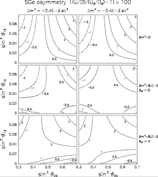
Figure 22: Isolines of the up-down electron asymmetry in the sub-GeV atmospheric neutrino sample, normalized to no-oscillation expectations. Left and right panels refer to normal and inverted hierarchy, respectively. Upper panels: $\delta m^{2}=0$; middle panel: $(\delta m^{2},\sin^{2}\theta_{12})$ fixed at their best-fit values and $\delta=0$; lower panel: as for the middle panel but with $\delta=\pi$.

Fig. 22 shows isolines of $100\times A_{e}$ for the SG$e$ sample, plotted in the $(\sin^{2}\theta_{23},\sin^{2}\theta_{13})$ plane at fixed $\Delta m^{2}=2.4\times 10^{-3}$ eV², for both normal hierarchy ($+\Delta m^{2}$, left panels) and inverse hierarchy ($-\Delta m^{2}$, right panels). In both hierarchies, we consider first the “academic” case $\delta m^{2}=0$ (top panels), then we switch on the LMA parameters $(\delta m^{2},\sin^{2}\theta_{12})$ at their best-fit values, for the the two CP-conserving cases $\delta=0$ (middle panels) and $\delta=\pi$ (bottom panels). The isolines in the upper panels reflect the behavior of the $\Delta_{1}$ term, which is positive (negative) for $s^{2}_{23}>1/r$ ($<1/r$), and vanishes for $\theta_{13}\to 0$, with a weak dependence on the hierarchy through $\tilde{\theta}_{13}$. In the middle panel, subleading LMA effects are operative through $\Delta_{2}$ and $\Delta_{3}$. The variation of $A_{e}$ in sign and magnitude is now more modest as $s_{23}^{2}$ increases, since the variation of the $\Delta_{1}$ term is now partially compensated by the opposite variation of the $\Delta_{2}$ term. In particular, the term $\Delta_{2}$ is responsible for nonzero values of $A_{e}$ at $\theta_{13}=0$, which break the $\theta_{23}$ octant symmetry [133], as also phenomenologically observed in Fig. 15. The difference between the middle and bottom panels is due to the interference term $\Delta_{3}$, which is typically negative (positive) for $\delta=0$ ($\delta=\pi$), and thus either adds or subtracts to $\Delta_{1}$ and $\Delta_{2}$ in the two cases. However, for $\theta_{13}=0$ the values of $A_{e}$ basically coincide in all middle and bottom panels, since the only surviving term ($\Delta_{2}$) carries no dependence on the hierarchy or the CP parity. From the results in Fig. 22 we learn that: (1) subleading $\delta m^{2}$-induced effects are of the same size of $\theta_{13}$-induced effects in the SG sample, so none can be neglected in a precise $3\nu$ oscillation analysis; (2) for nonzero values of both $\delta m^{2}$ and $\theta_{13}$, the sub-GeV electron asymmetry is typically more pronounced (and positive) for $\delta=\pi$, as compared with the case $\delta=0$; one can thus expect the latter case to be slightly disfavored in a global fit (since the SG$e$ data show a slight asymmetry, see Fig. 18); (3) in any case, the electron asymmetry is typically at the percent or sub-percent level for $\sin^{2}\theta_{13}<\mathrm{few}\%$; therefore, statistical and systematic uncertainties need to be reduced at this extraordinary small level in order to really “observe” the effects in future atmospheric neutrino experiments [134].

Fig. 23 shows our numerical calculation of the up-down electron asymmetry for the SK multi-GeV sample. The six panels refer to the same cases as in Fig. 22. In the MG$e$ sample, the terms $\Delta_{2}$ and $\Delta_{3}$ are small, and there is little dependence on $\delta m^{2}$ and on the CP parity (top, middle and bottom panels being quite similar). The dominant $\Delta_{1}$ term makes the asymmetry generally positive, and with significant dependence on the hierarchy (left vs right panels) through $\tilde{\theta}_{13}$. The MG$e$ asymmetry can be of $O(10\%)$ and thus relatively large; with some luck, such asymmetry might be seen in future large Cherenkov detectors if $\theta_{13}$ is not too small (see, e.g., [145] and refs. therein). In any case, one can expect some dependence of the current SK fit on the hierarchy through multi-GeV events (see also [137] for older data); it is difficult, however, to “predict” which of the two hierarchies (normal or inverted) is currently preferred, since large statistical fluctuations make the zenith-angle pattern of SK MG$e$ data somewhat erratical (see Fig. 18).

We conclude this Section with a brief note on subleading effects in K2K (which have been numerically included throughout this work). For $\theta_{13}=0$, it is easy to derive that, in vacuum,

$$P_{\mu\mu}^{\mathrm{K2K}}\simeq 1-\sin^{2}2\theta_{23}\sin^{2}\left(\frac{\Delta m^{2}-\frac{\delta m^{2}}{2}\cos\theta_{12}}{4E}\,L\right)\ ,$$ (51)

at first order in $\delta m^{2}/\Delta m^{2}$. It is also not difficult to check that this formula is not significantly affected by matter effects, as far as $A\gg\delta m^{2}$, which is true for most of the K2K event spectrum. The $\theta_{23}$ octant-symmetry of the above equation is responsible for the appearance of two degenerate best-fits in the K2K analysis of Fig. 16. The above equation is not invariant under a change of hierarchy [146] ($+\Delta m^{2}\to-\Delta m^{2}$), which leads to a (really tiny) relative change of the oscillation phase equal to $\pm(\delta m^{2}/2)\cos\theta_{12}/\Delta m^{2}\simeq 0.6\%$; this change does not produce graphically observable effects in Fig. 16. Although very small, these and other subleading K2K effects (e.g., those arising for both $\theta_{13}$ and $\delta m^{2}$ nonzero) have been kept in the analysis, in order to be consistent with the atmospheric neutrino data analysis (where such effects have also been included, as already discussed), and in order to show explicitly their impact on the global SK+K2K+CHOOZ analysis presented in the next section.

4.3 SK, K2K and CHOOZ constraints ($\theta_{13}$ free)

In this section we present the results of our analysis of SK+K2K+CHOOZ data for unconstrained values of $(\Delta m^{2},\sin^{2}\theta_{23},\sin^{2}\theta_{13})$, and for fixed values $(\delta m^{2},\sin^{2}\theta_{12})=(8\times 10^{-5}\mathrm{\ eV^{2}},0.314)$ in all the three data samples. There are four discrete subcases in our analysis, corresponding to a change in hierarchy or CP parity:

$$[\mathrm{sign}(\Delta m^{2})=\pm 1]\otimes[\cos\delta=\pm 1]\ .$$ (52)

In particular we remind that, in this work, we do not consider generic values of $\delta$, but only the two inequivalent CP-conserving cases ($\delta=0$ and $\delta=\pi$). They are related by the transformation $+s_{13}\to-s_{13}$ which, of course, does not mean that $s_{13}$ can be negative, but just that $\cos\delta s_{13}$ can change sign. Since the two cases smoothly merge for $s_{13}\to 0$, we think it useful to show the results of our analysis also in terms of the variable $\cos\delta\,\sin\theta_{13}$, i.e., of $\pm\sin\theta_{13}$, for both normal and inverted hierarchy.

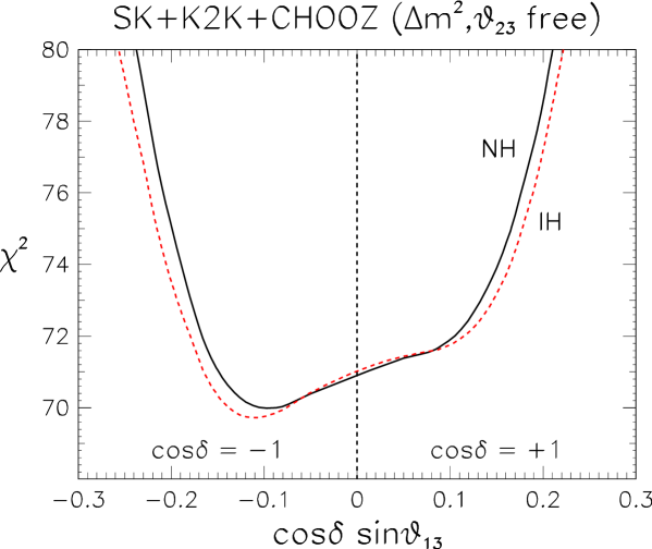
Figure 24: Three-neutrino analysis of SK+K2K+CHOOZ data, including subleading LMA effects. The results, marginalized with respect to $(\Delta m^{2},s^{2}_{23})$ and shown in terms of the $\chi^{2}(s_{13})$ function for both $\cos\delta=-1$ (left half of the panel) and $\cos\delta=+1$ (right part of the panel). The two CP-conserving cases $\cos\delta=\pm 1$ smoothly merge at $s_{13}=0$ (vertical dotted line). The solid and dashed curves refer to normal and inverted hierarchy, respectively.

Figure 24 shows the $\chi^{2}$ function from the SK+K2K+CHOOZ fit, in terms of $\cos\delta\,\sin\theta_{13}$, for marginalized $(\Delta m^{2},\sin^{2}\theta_{23})$ parameters. The solid and dashed curves correspond to normal and inverted hierarchy, respectively, while their left and right parts correspond to $\delta=\pi$ and $\delta=0$, respectively. Notice that the solid and dashed curves do not exactly coincide at $\theta_{13}=0$, since for $\delta m^{2}>0$ there is a very weak dependence on the hierarchy even at $\theta_{13}=0$ in reactor [85, 147], accelerator [146], and atmospheric [148] neutrino oscillations. The difference is, however, really tiny within the current global analysis ($\Delta\chi^{2}\simeq 0.2$ at $s_{13}=0$). The absolute $\chi^{2}$ minimum is reached in the left half of the figure ($\delta=\pi$) for $\sin\theta_{13}\simeq 0.1$; the minimum in the right half ($\delta=0$), which is reached for $\theta_{13}=0$, is only slight higher $(\Delta\chi^{2}<1)$. The slight difference between these two CP-conserving cases is mainly due to sub-GeV SK events, as discussed in the comments to Fig. 22. Finally, normal and inverted hierarchies give basically the same results for small values of $s_{13}$ (say, $<0.1$), while the latter hierarchy is slightly preferred for higher values of $s_{13}$. The fit becomes rapidly worse for $s_{13}\sim 0.2$ or higher. Figure 24 nicely summarizes our current (unfortunately weak) sensitivity to the neutrino mass hierarchy and to the extremal (CP-conserving) cases $\delta=0$ and $\delta=\pi$.

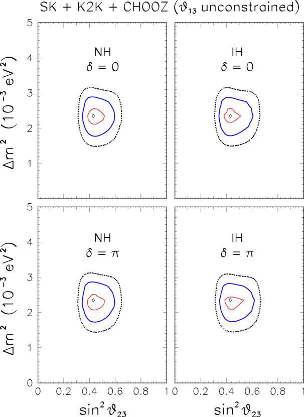
Figure 25: Three-neutrino analysis of SK+K2K+CHOOZ data, including subleading LMA effects. The results, marginalized with respect to $s^{2}_{13}$, are shown in the $(\Delta m^{2},s^{2}_{23})$ plane for the two hierarchies (left and right) and the two CP-conserving cases (top and bottom).

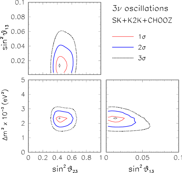
Figure 26: Three-neutrino analysis of SK+K2K+CHOOZ data, including subleading LMA effects. The results are shown as projections of the $(\Delta m^{2},s^{2}_{23},s^{2}_{13})$ allowed regions (at 1, 2, and $3\sigma$), marginalized with respect to the four cases $[\cos\delta=\pm 1]\otimes[\mathrm{sign}(\pm\Delta m^{2})=\pm 1]$.

Figure 25 shows the parameter space orthogonal to the one in Fig. 24, i.e., the bounds on $(\Delta m^{2},\sin^{2}\theta_{23})$ for marginalized $\theta_{13}$, in each of the four cases in Eq. (52). The differences between such cases are very small. Figure 24 and 25 confirm that our current sensitivity to the subleading effects—which distinguish the four subcases in Eq. (52)—is not statistically appreciable yet. Therefore, it makes sense to make a further marginalization over the four subcases, by minimizing the SK+K2K+CHOOZ function with respect to hierarchy and CP parity. The results are shown in Fig. 26, in terms of the projections of the $(\Delta m^{2},\sin^{2}\theta_{23},\sin^{2}\theta_{13})$ region allowed at 1, 2, and $3\sigma$ onto each of the coordinate planes. The best fit is reached for nonzero $\theta_{13}$ (as expected from Fig. 24), but $\theta_{13}=0$ is allowed within less than $1\sigma$. The preferred value of $\sin^{2}\theta_{23}$ remains slightly below maximal mixing. The best-fit value of $\Delta m^{2}$ is $2.4\times 10^{-3}$ eV². Notice that the correlations among the three parameters in Fig. 26 are very weak.

5 Global analysis of oscillation data

The results of the global analysis of solar and KamLAND data (Sec. 3.4) and of SK+K2K+CHOOZ data (Sec. 4.3) can now be merged to provide our best estimates of the five parameters $(\delta m^{2},\Delta m^{2},\theta_{12},\theta_{13},\theta_{23})$, marginalized over the four cases in Eq. (52). The bounds will be directly shown in terms of the “number of sigmas”, corresponding to the function $(\Delta\chi^{2})^{1/2}$ for each parameter.

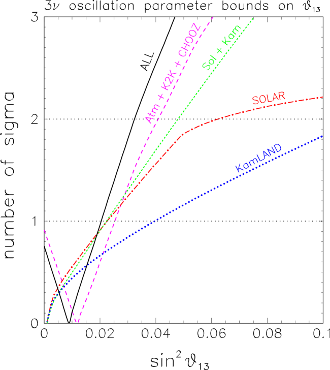
Figure 27: Global three-neutrino analysis of oscillation data. Bounds on $s^{2}_{13}$ are shown in terms of $n\sigma=\sqrt{\Delta\chi^{2}}$ for KamLAND (dotted curve), solar (dot-dashed curve), solar+KamLAND (short-dashed curve), SK+K2K+CHOOZ (long-dashed curve) and all data combined (solid curve). In each case, the continuous parameters $(\Delta m^{2},s^{2}_{23},s^{2}_{13})$ and—if applicable—the discrete parameters $[\cos\delta=\pm 1]\otimes[\mathrm{sign}(\pm\Delta m^{2})=\pm 1]$ are marginalized away.

Figure 27 shows our global bounds on $\sin^{2}\theta_{13}$, as coming from all data (solid line) and from the following partial data sets: KamLAND (dotted), solar (dot-dashed), solar+KamLAND (short-dashed) and SK+K2K+CHOOZ (long-dashed). Only the latter set, as observed before, gives a weak indication for nonzero $\theta_{13}$. Interestingly, solar+KamLAND data are now sufficiently accurate to provide bounds which are not much weaker than the dominant SK+K2K+CHOOZ ones, also because the latter slightly prefer $\theta_{13}>0$ as best fit, while the former do not.

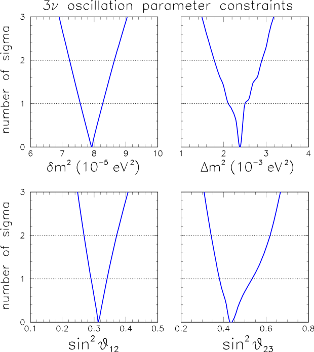
Figure 28: Global three-neutrino analysis of oscillation data. Bounds on each of the parameters $\delta m^{2}$, $\Delta m^{2}$, $\sin^{2}\theta_{12}$, and $\sin^{2}\theta_{23}$ are shown in terms of $n\sigma=\sqrt{\Delta\chi^{2}}$. In each plot, all parameters but the one in abscissa are marginalized away.

Figure 28 shows our global bounds on the four mass-mixing parameters which present both upper and lower limits with high statistical significance. Notice that the accuracy of the parameter estimate is already good enough to lead to almost “linear” errors, especially for $\delta m^{2}$ and $\sin^{2}\theta_{12}$. For $\Delta m^{2}$ and $\sin^{2}\theta_{23}$, such “linearity” is somewhat worse in the region close to the best fit (say, within $\pm 1\sigma$), and thus $2\sigma$ (or $3\sigma$) errors should be taken as reference.

We summarize our results through the following $\pm 2\sigma$ ranges (95% C.L.) for each parameter:

$$\sin^{2}\theta_{13} = 0.9^{+2.3}_{-0.9}\times 10^{-2}\ ,$$ (53)

$$\delta m^{2} = 7.92\,(1\pm 0.09)\times 10^{-5}\mathrm{\ eV}^{2}\ ,$$ (54)

$$\sin^{2}\theta_{12} = 0.314\,(1^{+0.18}_{-0.15})\ ,$$ (55)

$$\Delta m^{2} = 2.4\,(1^{+0.21}_{-0.26})\times 10^{-3}\mathrm{\ eV}^{2}\ ,$$ (56)

$$\sin^{2}\theta_{23} = 0.44\,(1^{+0.41}_{-0.22})\ .$$ (57)

Notice that the lower uncertainty on $\sin^{2}\theta_{13}$ is purely formal, corresponding to the positivity constraint $\sin^{2}\theta_{13}\geq 0$. Correlations among parameters are not quoted, being currently small (as already observed).

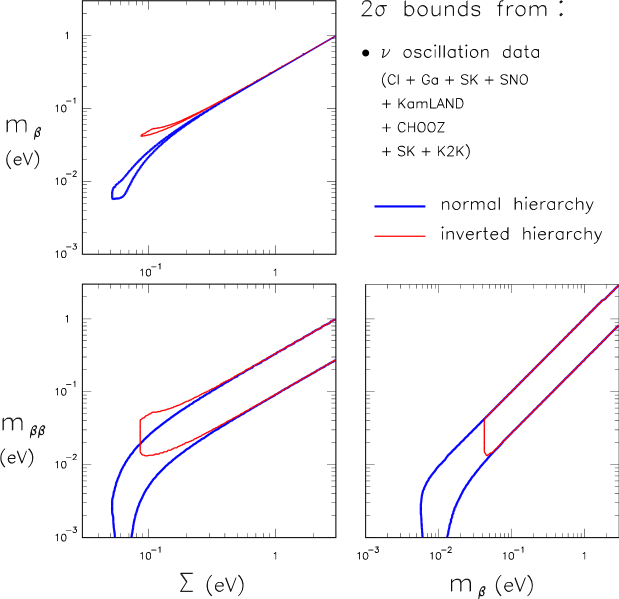
Figure 29: Regions allowed at $2\sigma$ by the global analysis of neutrino oscillation data in the parameter space of non-oscillatory observables $(m_{\beta},m_{\beta\beta},\Sigma)$. The regions are projected onto the three coordinate planes for both normal hierarchy (thick curves) and inverted hierarchy (thin curves).

The above bounds have been obtained from a global analysis of oscillation data (for $U=U^{*}$). They have, however, an impact also on non-oscillation observables. In particular, the smallness of the squared mass splittings induces significant correlations on the three parameters $(m_{\beta},m_{\beta\beta},\Sigma)$ which are sensitive to absolute neutrino masses (see [55] and references therein). Figure 29 shows the updated $2\sigma$ allowed bands in each of the three corresponding coordinate planes, for both normal and inverted hierarchy. There is an evident positive correlation, especially between $m_{\beta}$ and $\Sigma$; the correlation is less pronounced when it involves $m_{\beta\beta}$, due to our ignorance of the Majorana phases $\phi_{2}$ and $\phi_{3}$ (that we take as free parameters). The two hierarchies split up only at very low values of the observables, where mass splittings start to be of the order of the absolute masses (non-degenerate cases). Non-oscillation data on $m_{\beta}$, $m_{\beta\beta}$ and $\Sigma$ can reduce the allowed parameter space in Fig. 29, hopefully leading to a single solution and thus to the determination of the absolute neutrino masses. Such data are discussed in the next Section.

6 Global analysis of oscillation and non-oscillation data

In this Section we discuss first non-oscillation data on the three observables $(m_{\beta},m_{\beta\beta},\Sigma)$, and then show how these data further constrain and reduce the allowed regions in Fig. 29. As we shall see, when all the data are taken at face value, no combination is possible: a strong tension arises, indicating that either some experimental information or their theoretical interpretation is wrong or biased. In particular, it appears difficult to reconcile [55] the claimed $0\nu 2\beta$ signal [47] and the most recent upper bounds on $\Sigma$ from precision cosmology [41, 42, 43]. However, relaxing one of either pieces of data reduces the tension and allows a global combination, which can be valuable for prospective studies [55].

Needless to say, the relations between the variables $(m_{\beta},m_{\beta\beta},\Sigma)$ have been subject to intensive studies, which form a large specialized literature on absolute neutrino mass observables. We refer the reader to the review papers [38, 39, 53, 67, 69, 149] for extensive bibliographies, and to the articles [55, 57, 150] for recent up-to-date discussions.

6.1 Bounds on $m_{\beta}$

Experimental constraints on the effective electron neutrino mass $m_{\beta}$ have been recently presented [36] for the Mainz and Troitsk tritium $\beta$-decay experiments. The experimental values are consistent with zero within errors. Their combined upper bound at $2\sigma$ has been estimated in [55] as:

$$m_{\beta}<1.8~{}\mathrm{eV}\ (\mathrm{Mainz}+\mathrm{Troitsk})\ ,$$ (58)

which is less conservative than the $3$ eV upper limit recommended in [1]. It should be mentioned that the Troitsk results are to be taken with some caution, being affected by an unexplained anomaly (namely, a fluctuating excess of counts near the endpoint) [36]. However, as we will see, upper limits on $m_{\beta}$ in the 2–3 eV range are, in any case, too weak to contribute significantly to the current global fit in the $(m_{\beta},m_{\beta\beta},\Sigma)$ parameter space, so that “conservativeness” is not (yet) an issue in this context.

6.2 Bounds on $m_{\beta\beta}$

Neutrinoless double beta decay processes of the kind $(Z,A)\to(Z+2,A)+2e^{-}$ have been searched in many experiments with different isotopes, yielding negative results (see [39, 149] for reviews). Recently, members of the Heidelberg-Moscow experiment have claimed the detection of a $0\nu 2\beta$ signal from the ⁷⁶Ge isotope [46, 47]. If this signal is entirely due to light Majorana neutrino masses, the $0\nu 2\beta$ half-life $T$ is related to the $m_{\beta\beta}$ parameter by the relation

$$m^{2}_{\beta\beta}=\frac{m^{2}_{e}}{C_{mm}T}\ ,$$ (59)

where $m_{e}$ is the electron mass and $C_{mm}$ is the nuclear matrix element for the considered isotope [39].

Unfortunately, theoretical uncertainties on $C_{mm}$ are rather large (see e.g. [39]), and their—somewhat arbitrary—estimate is matter of debate (see [151, 152, 153] and refs. therein). In [55] we adopted a naive but very conservative estimate, by defining the range spanned by “extremal” published values of $C_{mm}$ as an “effective $3\sigma$ range,” thus obtaining $\log_{10}(C_{mm}/\mathrm{y}^{-1})=-13.36\pm 0.97$ (at $\pm 3\sigma$). Here we prefer to adopt the results of a recent detailed discussion of the nuclear model uncertainties for $C_{mm}$, performed within the (Renormalized) Quasiparticle Random Phase Approximation, and calibrated to known $2\nu\beta\beta$ decay rates [154]. For our purposes, we cast the results of such promising approach [154] in the form $\log_{10}(C_{mm}/\mathrm{y}^{-1})=-13.36\pm 0.15$ (at $\pm 3\sigma$), where systematic coupling constant uncertainties ($g_{A}=1$–1.25, see [154]) have been included. This “new” range for $C_{mm}$ has (accidentally) the same central value as before, but with significantly reduced errors. Under the assumption of a positive $0\nu 2\beta$ signal [47], we then derive that

$$\log_{10}(m_{\beta\beta}/\mathrm{eV})=-0.23\pm 0.14\ (2\sigma)\ ,$$ (60)

i.e., $0.43<m_{\beta\beta}<0.81$ (at $2\sigma$, in eV). See also [55] for our previous (more conservative) estimated range.

The claim in [46, 47] has been subject to strong criticism, especially after the first publication [45] (see [39, 149] and refs. therein). Therefore, we will also consider the possibility that $T=\infty$ is allowed (i.e., that there is no $0\nu 2\beta$ signal), in which case the experimental lower bound on $m_{\beta\beta}$ disappears, and only the upper bound remains. In conclusion, we adopt the following two possible $0\nu 2\beta$ inputs for our global analysis:

$$\log_{10}(m_{\beta\beta}/\mathrm{eV}) = -0.23\pm 0.14\ (0\nu 2\beta\mathrm{\ signal\ assumed})\ ,$$ (61)

$$\log_{10}(m_{\beta\beta}/\mathrm{eV}) = -0.23^{+0.14}_{-\infty}\ (0\nu 2\beta\mathrm{\ signal\ not\ assumed})\ ,$$ (62)

where errors are at $2\sigma$ level. Concerning the unknown Majorana phases $\phi_{2}$ and $\phi_{3}$ in Eq. (15), we simply assume that they are independent and uniformly distributed in the range $[0,\pi]$, which covers all physically different cases in $m_{\beta\beta}$.

6.3 Bounds on $\Sigma$

The neutrino contribution to the overall energy density of the universe can play a relevant role in large scale structure formation, leaving key signatures in several cosmological data sets. More specifically, neutrinos suppress the growth of fluctuations on scales below the horizon when they become non relativistic. Massive neutrinos of a fraction of eV would therefore produce a significant suppression in the clustering on small cosmological scales. Data on large scale structures, combined with Cosmic Microwave Background (CMB) and other precision astrophysical data, can thus constrain the sum of neutrino masses $\Sigma$ (see [44, 89, 155, 156, 157] for recent reviews).

In this work we use the bounds on $\Sigma$ previously obtained in collaboration with other authors in [55], to which we refer the reader for technical details. We briefly remind that the experimental input used in [55] included CMB data from the Wilkinson Microwave Anisotropy Probe (WMAP) [41], large scale structure data [42] from the 2 degrees Fiels (2dF) Galaxy Redshift Survey [158] and, optionally, constraints on mall scales from the recent Lyman $\alpha$ (Ly$\alpha$) forest data of the Sloan Digital Sky Survey (SDSS) [159]. The latter data have a strong impact on the current upper bounds on $\Sigma$ [43], but are also affected by large systematics, which deserve further study [43, 159]. As in [55], we conservatively quote (and use) upper bounds on $\Sigma$ both with and without such Ly$\alpha$ forest data; in particular, the $2\sigma$ upper bounds from [55] read:

$$\Sigma < 0.5\mathrm{\ eV\ (with\ Ly}\alpha\mathrm{\ data)}\ ,$$ (63)

$$\Sigma < 1.4\mathrm{\ eV\ (without\ Ly}\alpha\mathrm{\ data)}\ .$$ (64)

6.4 Impact of non-oscillation observables

The experimental limits on the non-oscillation observables $(m_{\beta},m_{\beta\beta},\Sigma)$, previously reported in terms of $2\sigma$ ranges, are appropriately combined with oscillation data through $\Delta\chi^{2}$ functions [55]. Although such combination can provide allowed regions at any confidence level, in the following we shall continue to show only $2\sigma$ bounds for simplicity.

Figure 30 shows the impact of all the available non-oscillation data, taken at face value, in the parameter space $(m_{\beta\beta},\Sigma)$. Bounds on the third observable $m_{\beta}$ are projected away, being too weak to alter the discussion of the results in this figure. The horizontal band is allowed by the positive $0\nu 2\beta$ experimental claim [47] equipped with the nuclear uncertainties of [154] through Eq. (61). The slanted bands (for normal and inverted hierarchy) are allowed by all other neutrino data, i.e., by the combination of neutrino oscillation constraints (as in Fig. 29) and of astrophysical CMB+2dF+Ly$\alpha$ constraints through Eq. (63). The tight cosmological upper bound on $\Sigma$ prevents the overlap between the slanted and horizontal bands at $2\sigma$, indicating that no global combination of oscillation and non-oscillation data is possible in the sub-eV range. The “discrepancy” is even stronger than it was found in [55], due to the adoption of smaller $0\nu 2\beta$ nuclear uncertainties [154]. It is premature, however, to derive any definite conclusion as to which piece of the data or of the $3\nu$ scenario is “wrong” in this conflicting picture. Further experimental and theoretical research is needed to clarify absolute neutrino observables in the sub-eV range.

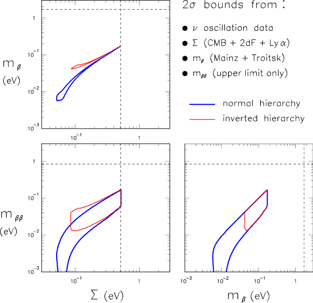
Figure 31: Analysis of oscillatory and non-oscillatory observables in the parameter space $(m_{\beta},m_{\beta\beta},\Sigma)$, including all data but the claimed lower bound from $0\nu 2\beta$ searches.

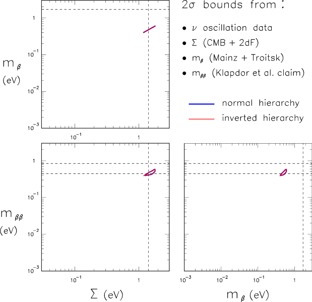
Figure 32: Analysis of oscillatory and non-oscillatory observables in the parameter space $(m_{\beta},m_{\beta\beta},\Sigma)$, including the claimed $0\nu 2\beta$ signal but excluding the recent Ly$\alpha$ forest data. The contours of the allowed regions for normal and inverted spectrum hierarchy overlap (regime of degenerate spectrum).

It is tempting, however, to see if the removal of some pieces of data can relax the tension in Fig. 30. The effect of removing only the lower bound on $m_{\beta\beta}$ through Eq. (62) is shown in Fig. 31. Of the three remaining upper bounds on $m_{\beta}$, on $m_{\beta\beta}$, and on $\Sigma$, the latter is definitely dominant, and implies that future beta and double-beta decay searches should push their sensitivity below 0.2 eV, irrespective of the hierarchy. Conversely, the effect of removing only the Ly$\alpha$ forest data through Eq. (64) is shown in Fig. 32. In this case, the combination of the claimed $0\nu 2\beta$ signal with oscillation data dominates the global fit, and “predicts” the observation of $\Sigma\simeq 1.5$ eV and $m_{\beta}\simeq 0.5$ eV within formally small uncertainties (about $\pm 20\%$ at $2\sigma$). These predictions would really be “around the corner” from the observational viewpoint, both for $\Sigma$ [89] and for $m_{\beta}$ [36]. Future searches are expected to clarify the—currently controversial—situation about absolute mass observables in the sub-eV range, as depicted in Figs. 30–32.

7 Conclusions

We have performed a comprehensive phenomenological analysis of a vast amount of data from neutrino flavor oscillation and non-oscillation searches, including solar, atmospheric, reactor, accelerator, beta-decay, double-beta decay, and precision astrophysical observations. In the analysis, performed within the standard scenario with three massive and mixed neutrinos (for both mass hierarchies and for the two inequivalent CP-conserving cases), we have paid particular attention to implement subleading oscillation effects in numerical calculations, and to carefully include all known sources of uncertainties in the statistical comparison of theoretical predictions and experimental data. We have discussed the impact of solar and reactor data on the parameters $(\delta m^{2},\sin^{2}\theta_{12},\sin^{2}\theta_{13})$, as well as the impact of atmospheric and reactor data on $(\Delta m^{2},\sin^{2}\theta_{23},\sin^{2}\theta_{13})$. The bounds from the global analysis of oscillation data have been summarized, and several subleading effects have been discussed. Finally, we have analyzed the interplay between the oscillation parameters $(\delta m^{2},\Delta m^{2},\sin^{2}\theta_{12},\sin^{2}\theta_{23},\sin^{2}\theta_{13})$ and the non-oscillation observables sensitive to absolute neutrino masses ($m_{\beta},m_{\beta\beta},\Sigma$), both with and without controversial data, which may or may not allow a reasonable global combination of all data. The detailed results discussed in this review article represent a state-of-the-art, accurate and up-to-date (as of August 2005) overview of the neutrino mass and mixing parameters within the standard three-generation framework.

Appendix

In this Appendix we report—for more expert readers—additional technical information about the $\chi^{2}$ analysis of each data sample, which has been used to derive partial and global parameter bounds in this work. In particular, global constraints have been obtained by adding up all $\chi^{2}$ contributions and by scanning the (CP-conserving) $3\nu$ mass-mixing parameter space

$$\mathbf{p}=\{\pm\Delta m^{2},\delta m^{2},s^{2}_{23},s^{2}_{13},s^{2}_{12},\cos\delta=\pm 1\}\ ,$$ (65)

with allowed regions being derived through $\Delta\chi^{2}$ cuts with respect to the best-fit point. As discussed in the preceding Sections of this review, some data samples are actually not sensitive to all of the above parameters; the relevant variables in $\mathbf{p}$ will be explicitly emphasized in the following subsections.

7.1 CHOOZ

The CHOOZ experiment [32] has measured the positron energy spectra induced by $\overline{\nu}_{e}$’s produced by two nuclear reactors located at $L_{1}=1114.6$ km and $L_{2}=997.9$ km from the detector. Each of the two spectra is divided in 7 energy bins, for a total of 14 event rate bins. In our analysis, such data are included through the following $\chi^{2}$ function:

$$\chi^{2}_{\mathrm{CHOOZ}}(\mathbf{p})=\min_{\alpha}\left\{\sum_{i,j=1}^{14}[R_{i}^{\mathrm{expt}}-\alpha R_{i}^{\mathrm{theo}}(\mathbf{p})]\,[\sigma^{2}_{ij}]^{-1}[R_{j}^{\mathrm{expt}}-\alpha R_{j}^{\mathrm{theo}}(\mathbf{p})]+\left(\frac{\alpha-1}{\sigma_{\alpha}}\right)^{2}\right\}\ ,$$ (66)

where $R_{i}^{\mathrm{expt}}$ and $R_{i}^{\mathrm{theo}}$ are the observed and predicted rates in each bin, respectively, and $\alpha$ is an overall normalization factor with uncertainty $\sigma_{\alpha}=2.7\times 10^{-2}$. The squared error matrix is defined as [32]:

$$\sigma^{2}_{ij}=\delta_{ij}(s^{2}_{i}+u^{2}_{i})+(\delta_{i,j-7}+\delta_{i,j+7})c^{2}_{i}\ ,$$ (67)

where $s_{i}$ and $u_{i}$ represent statistical errors and uncorrelated systematic errors, respectively, while the $c_{i}$’s represent fully correlated systematic errors between equal-energy bins in the two reactor spectra. The theoretical rate in each bin is estimated as

$$R_{i}^{\mathrm{theo}}=R_{i}^{0}\cdot\langle P_{ee}(\mathbf{p})\rangle_{i}\ ,$$ (68)

where $R_{i}^{0}$ is the no-oscillation rate, and $\langle P_{ee}(\mathbf{p})\rangle_{i}$ is the $\overline{\nu}_{e}$ survival probability, averaged over the appropriate energy range for the i-$th$ bin, taking into account the detector energy resolution and the reactor core size. Numerical values for the rates $R_{i}^{0}$ and the errors $s_{i}$, $u_{i}$, and $c_{i}$, can be found in [32].

We have checked that, through the above $\chi^{2}$ function, we can accurately reproduce the published CHOOZ limits (analysis A of [32]) in the parameter space $\mathbf{p}=\{\Delta m^{2},s^{2}_{13}\}$. For the sake of precision, in this work we have used the most general $3\nu$ parameter space for CHOOZ [85]

$$\mathbf{p}=\{\pm\Delta m^{2},\delta m^{2},s^{2}_{13},s^{2}_{12}\}\ .$$ (69)

The effect of the subdominant parameters $[\delta m^{2},s^{2}_{12},\mathrm{sign}(\pm\Delta m^{2})]$ is, however, rather small in the current data analysis.

7.2 KamLAND

The published KamLAND energy spectrum [20, 21] contains 258 events (background+signal), which we analyze through a maximum-likelihood approach [20], described in detail in [93]. In particular, the KamLAND (KL) $\chi^{2}$ function is defined as

$$\chi^{2}_{\mathrm{KL}}({\mathbf{p}})=-2\ln\,\max_{(\alpha,\alpha^{\prime},\alpha^{\prime\prime})}\mathcal{L}_{\mathrm{KL}}(\mathbf{p},\alpha,\alpha^{\prime},\alpha^{\prime\prime})\ ,$$ (70)

where $\alpha$ parametrizes a systematic energy-scale offset, while $\alpha^{\prime}$ and $\alpha^{\prime\prime}$ represent free normalization factors for two (poorly constrained) background components [93]. The above likelihood function is factorized as

$$\mathcal{L}_{\mathrm{KL}}(\mathbf{p},\alpha,\alpha^{\prime},\alpha^{\prime\prime})=\mathcal{L}_{\mathrm{rate}}(\mathbf{p},\alpha,\alpha^{\prime},\alpha^{\prime\prime})\times\mathcal{L}_{\mathrm{shape}}(\mathbf{p},\alpha,\alpha^{\prime},\alpha^{\prime\prime})\times\mathcal{L}_{\mathrm{syst}}(\alpha)\ ,$$ (71)

where the first, second, and third term embed the probability distribution for the total rate, for the spectrum shape, and for the systematic offset $\alpha$, respectively; explicit expressions are reported in [93]. In particular, the spectrum shape term is further factorized into the probability distributions $D(E_{i})$ for finding the 258 KamLAND events with observed energies $\{E_{i}\}_{i=1,\dots,258}$:

$$\mathcal{L}_{\mathrm{shape}}=\prod_{i=1}^{258}D(E_{i})\ .$$ (72)

A final remark is in order. In [93] the KamLAND analysis was performed in the $2\nu$ parameter space $\mathbf{p}=\{\delta m^{2},s_{12}\}$, where the published bounds [20, 21] have been accurately reproduced. In this work we have instead used the full $3\nu$ parameter space relevant for KamLAND,

$$\mathbf{p}=\{\delta m^{2},s^{2}_{12},s^{2}_{13}\}\ .$$ (73)

We have checked, for a number of representative points in the $3\nu$ parameter space, that the addition of KamLAND time-variation information [93] does not alter in any appreciable way the KamLAND constraints in such $3\nu$ space.

7.3 SK atmospheric data

Our SK data analysis includes the zenith angle distributions of leptons induced by atmospheric neutrinos, for a total of 55 bins, as discussed in [117]. With respect to [117], we have updated the experimental event rates and their statistical errors $\{R^{\mathrm{expt}}_{n}\pm\sigma_{n}^{\mathrm{stat}}\}$ from [26]. We also use three-dimensional neutrino fluxes [126] for the calculation of the theoretical rates $R_{n}^{\mathrm{theo}}(\mathbf{p})$. For convenience, we normalize both the experimental and theoretical rates to their no-oscillation value in each bin, as shown in Fig. 18. We consider eleven sources of systematic errors, which can produce a shift of the theoretical predictions through a set of “pulls” $\{\xi_{k}\}_{k=1,\dots,11}$ [117],

$$\overline{R}_{n}^{\mathrm{theo}}(\mathbf{p})=R_{n}^{\mathrm{theo}}(\mathbf{p})+\sum_{k=1}^{11}\xi_{k}c_{n}^{k}\ ,$$ (74)

where the response $c_{n}^{k}$ of the $n$-th bin to the $k$-th systematic source is numerically given in [117]. The $\chi^{2}$ function is then obtained by minimization over the $\xi_{k}$’s (which are partly correlated through a matrix $\rho^{\mathrm{syst}}_{hk}$ [117]),

$$\chi^{2}_{\mathrm{SK}}(\mathbf{p})=\min_{\{\xi_{k}\}}\left[\sum_{n=1}^{55}\left(\frac{\overline{R}_{n}^{\mathrm{theo}}(\mathbf{p})-R_{n}^{\mathrm{expt}}}{\sigma_{n}^{\mathrm{stat}}}\right)^{2}+\sum_{k,h=1}^{11}\xi_{k}[\rho^{-1}_{\mathrm{syst}}]_{hk}\xi_{h}\right]\ .$$ (75)

Minimization leads to a set of linear equations in the $\xi_{k}$’s, which are solved numerically. The solution ${\overline{\xi}_{k}}$ can provide useful statistical information about the preferred systematic offsets and theoretical rate shifts, as discussed in Sec. 4.1.

Finally, the $3\nu$ parameter space used for the SK data analysis in this work is

$$\mathbf{p}=\{\pm\Delta m^{2},s^{2}_{23},s^{2}_{13},\cos\delta=\pm 1,\delta m^{2*},s^{2*}_{12}\}\ ,$$ (76)

where $\delta m^{2*}$ and $s^{2*}_{12}$ are the (fixed) best-fit values from the solar+KamLAND data analysis in Sec. 3.1. We have verified, in a number of representative points, that variations of these two parameters within their $\pm 2\sigma$ limits do not alter the SK atmospheric data analysis in any appreciable way.

7.4 K2K

In this work, the K2K analysis is based on a 6-bin energy spectrum as in [117], but including updated data [31, 129] as shown in Fig. 17. We cannot perform a K2K spectral analysis with finer binning (as the official one [31]) for lack of published information about bin-to-bin systematic errors and their correlations in the last data release. The $\chi^{2}$ definition is based on a pull approach (with 7 systematic error sources [117]), but the small number $N$ of events in each bin requires a Poisson statistics, implemented through [117]

$$\chi^{2}_{\mathrm{K2K}}(\mathbf{p})=\min_{\{\xi_{k}\}}\left[2\sum_{n=1}^{6}\left(\overline{N}_{n}^{\mathrm{theo}}-N_{n}^{\mathrm{expt}}-N_{n}^{\mathrm{expt}}\ln\frac{\overline{N}_{n}^{\mathrm{theo}}}{N_{n}^{\mathrm{expt}}}\right)+\sum_{k,h=1}^{7}\xi_{k}[\rho^{-1}_{\mathrm{syst}}]_{hk}\xi_{h}\ \right]\ ,$$ (77)

with shifted predictions

$$\overline{N}_{n}^{\mathrm{theo}}(\mathbf{p})=N_{n}^{\mathrm{theo}}(\mathbf{p})+\sum_{k=1}^{7}\xi_{k}c_{n}^{k}\ .$$ (78)

Numerical values for the K2K response functions $c_{n}^{k}$ and for the correlation matrix $\rho_{hk}^{\mathrm{syst}}$ are given in [117].

For the sake of precision, and for consistency in the SK+K2K(+CHOOZ) combination, we have used for K2K the same $3\nu$ parameter as for SK

$$\mathbf{p}=\{\pm\Delta m^{2},s^{2}_{23},s^{2}_{13},\cos\delta=\pm 1,\delta m^{2*},s^{2*}_{12}\}\ ,$$ (79)

although the subleading effects of the last two parameters are rather small in the K2K data analysis.

7.5 Solar neutrinos

The definition of the solar neutrino $\chi^{2}$ is rather complex, both because it includes 119 observables and 55 sources of systematics, and because it currently involves also correlations of statistical errors in the SNO salt data [17] and of systematic error sources in the BS05 (OP) solar model [98, 99, 100]. Here we will mainly highlight the differences of the new $\chi^{2}$ inputs, with respect to our previous discussion in [94].

The formal $\chi^{2}$ definition is based on a pull approach,

$$\chi^{2}_{\mathrm{sol}}(\mathbf{p})=\min_{\{\xi_{k}\}}\left[\sum_{n,m}^{119}x_{n}[\rho^{-1}]_{nm}x_{m}+\sum_{h,k}^{55}\xi_{h}[\rho^{-1}_{\mathrm{syst}}]_{hk}\xi_{k}\right]\ ,$$ (80)

where

$$x_{n}=\frac{\overline{R}_{n}^{\mathrm{theo}}(\mathbf{p})-R_{n}^{\mathrm{expt}}}{\sigma_{n}}\ ,$$ (81)

and

$$\overline{R}_{n}^{\mathrm{theo}}=R_{n}^{\mathrm{theo}}+\sum_{k=1}^{55}\xi_{k}c_{n}^{k}\ .$$ (82)

The presence of statistical error correlations ($\rho_{nm}\neq\delta_{nm}$) in the latest SNO data [17] does not spoil [95] the advantages of the pull approach discussed in [94] (where $\rho_{nm}=\delta_{nm}$). We remind that the parameter space used in the solar neutrino data analysis is

$$\mathbf{p}=\{\delta m^{2},s^{2}_{12},s^{2}_{13}\}\ ,$$ (83)

except for Fig. 13 and related comments, where the very weak sensitivity to $\pm\Delta m^{2}$ has been discussed.

In the following we briefly describe, in ascending order, the $n=1\dots 119$ observables and the $k=1\dots 55$ systematic error sources of the solar neutrino analysis.

7.5.1 Observables

$n=1$ (Chlorine rate). The Chlorine rate input [7, 12] is $R_{1}^{\mathrm{expt}}\pm\sigma^{\prime}_{1}=2.56\pm 0.23$ SNU. A $\mathbf{p}$-dependent cross-section error is added in quadrature to $\sigma^{\prime}_{1}$ (as described in [94]) to obtain the total uncorrelated error $\sigma_{1}$.

$n=2,3$ (Gallium total rate and winter-summer asymmetry). The Gallium (GALLEX/GNO+SAGE) input for the total rate is $R_{2}^{\mathrm{expt}}\pm\sigma^{\prime}_{2}=68.1\pm 3.75$ SNU [9, 11, 12]. A $\mathbf{p}$-dependent cross-section error is added in quadrature to $\sigma^{\prime}_{2}$ (as described in [94]) to obtain the total uncorrelated error $\sigma_{2}$. The combined (GALLEX/GNO+SAGE) input for the winter-summer asymmetry (corrected for geometrical eccentricity effects [118]) is $R_{3}\pm\sigma_{3}=-0.6\pm 7$ SNU [12].

$n=4,\dots,47$ (SK solar neutrino spectrum in energy and nadir angle). The analysis of the SK 44-bin spectrum [13] uses the same experimental input as described in appendix C of [94], but all the theoretically computed quantities have been updated (in each point of the parameter space $p$) to account for the new hep and ⁸B solar neutrino input in the BS05 (OP) model [98, 100].

${n=48,\dots,81}$ (SNO spectrum, pure D₂O phase). In this data set [15], events from NC, CC and ES scattering (and from various backgrounds) are not separated, and the global NC+CC+ES energy spectrum is analyzed. The spectrum information includes 34 bins (17 day + 17 night [15]) and is treated as described in appendix D of [94]. As for the above (SK) data set, the only update concerns theoretical calculations, in order to account for BS05 (OP) solar model hep and ⁸B input.

${n=82,\dots,119}$ (SNO CC spectrum and ES+NC rates, salt phase). In this recent SNO data set [17], the addition of salt has allowed a statistical separation of CC, NC and ES events. The CC spectrum includes 34 bins (17 day and 17 night, $n=82,\dots 115$). Four more data points concern the total NC rate (day and night, $n=116,117$) and ES rate (day and night, $n=118,119$). The experimental values for the rates and their statistical errors $(R_{n}^{\mathrm{expt}}\pm\sigma_{n})$ are taken from Table XXX (CC) and XXIV (NC+ES) of [17]. These are the only data where the (statistical) errors are correlated, namely, $\rho_{n,m>82}\neq\delta_{nm}$. The two ($19\times 19$) statistical correlation matrices for day and night data are taken from Tables XXXII and XXXIII of [17], respectively.

7.5.2 Systematics

${k=1,\dots,20}$ (Standard Solar Model systematics). In [94] 12 sources $X_{k}$ of systematic errors were considered in the input solar model, individually denoted as $S_{11}$, $S_{33}$, $S_{34}$, $S_{1,14}$, $S_{17}$, Lum, Opa, Diff, $C_{\mathrm{Be}}$, $S_{\mathrm{hep}}$, and $Z/X$, each source being affected by a relative error $\Delta X_{k}/X_{k}$ (see also [160] and refs. therein). With respect to [94], the first 11 systematic uncertainties are unchanged, except for the updated value of $\Delta X/X$ for $S_{17}$, currently set to 0.038 [161] (it was 0.106 in [94, 160]). The former systematic error source $Z/X$ (solar metallicity) is now separated [98] into 9 elemental uncertainties related to C, N, O, Ne, Mg, Si, S, Ar, and Fe, whose $\Delta X_{k}/X_{k}$ values are taken from the conservative estimate in Table 4 of [98]. Three among these new error sources (O, Ne, Ar) are fully correlated [98], and make the matrix $\rho^{\mathrm{syst}}_{hk}$ different from unity for (and only for) $h,k=14,15,19$. The 11+9=20 SSM systematic error sources $X_{k}$ affect the neutrino fluxes through log-derivatives $\alpha_{ik}$ (see [94, 160, 98]). For $k=1,\dots,11$, such derivatives are unchanged with respect to [94, 160]. For the new metallicity uncertainties ($k=12,\dots,20$), we take the log-derivatives from Table 1 of [98]. Finally, all SSM systematic uncertainties are propagated to the final $c_{n}^{k}$ values in each point of the parameter space, as described in [94].

$k=21$ (⁸B spectrum shape uncertainty). The treatment of this systematic error [119] (which affect all solar neutrino observables) is unchanged from [94].

${k=22,\dots,32}$ (SK spectrum) and ${k=33,\dots,39}$ (SNO no-salt spectrum). The SK spectrum data $\{R_{n}\}_{n=4\dots,47}$ are affected by 11 systematics $k=22,\dots,32$. Analogously, the SNO (pure D₂O phase, $\{R_{n}\}_{n=48,\dots,81}$) data are affected by 7 systematics. They are treated as described in [94].

${k=40,\dots,55}$ (SNO salt-phase systematics). The recent SNO data in the salt phase $\{R_{n}\}_{n=82,\dots,119}$ are affected (in equal way during day and night) by 16 sources of systematic errors [17]. The response function $c_{n}^{k}$ is numerically given in Table XXXIV of [17], in terms of (generally asymmetrical) upper and lower values $c_{n}^{k+}$ and $c_{n}^{k-}$. Such values cannot be incorporated at face value in a $\chi^{2}$ function, which postulates symmetrical uncertainties. As mentioned in Sec. 3, in the pull approach we solve this problem through the prescription suggested in [96], namely, by shifting the central values of the observables (through the error half-difference) and by attaching symmetrized (half-sum) systematic errors as

$$\overline{R}_{n}=R_{n}+\sum_{k=40}^{55}\frac{c_{n}^{k+}-c_{n}^{k-}}{2}+\sum_{k=40}^{55}\xi_{k}\frac{c_{n}^{k+}+c_{n}^{k-}}{2}\ \ \ (n=82,\dots,119)\ .$$ (84)

7.6 Observables sensitive to absolute neutrino masses

For the $\chi^{2}$ functions related to $m_{\beta}$, $m_{\beta\beta}$, and $\Sigma$, we refer the reader to the thorough discussion given in [55]. With respect to [55], in this work we have only reduced the theoretical nuclear uncertainty affecting $m_{\beta\beta}$, according to the recent results reported in [154] (see Sec. 6.2).

Figure 17: K2K event spectrum as a function of reconstructed neutrino energy. Data (as used in this work) are shown by dots with $\pm 1\sigma$ statistical error bars. The histograms represent our calculations for no oscillation (dotted), and for oscillations at the SK+K2K best fit in Fig. 16 (dashed: with no systematic shifts; solid: with systematic shifts allowed).

Figure 21: Representative examples of subleading three-neutrino effects in the SG$e$ and MG$e$ samples. See the text for details.

Figure 23: As in Fig. 22, but for multi-GeV neutrinos.

Figure 30: Analysis of oscillatory and non-oscillatory observables in the plane $(m_{\beta\beta},\Sigma)$. The $2\sigma$ horizontal band is preferred by the positive $0\nu 2\beta$ claim, while the slanted $2\sigma$ regions below are preferred by all other data (oscillation and cosmological data). The absence of overlap indicates tension among the data in the sub-eV range.

References

- [1] Review of Particle Physics, S. Eidelman et al., Phys. Lett. B 592, 1 (2004).
- [2] Z. Maki, M. Nakagawa, and S. Sakata, Prog. Theor. Phys. 28, 870 (1962); B. Pontecorvo, Zh. Eksp. Teor. Fiz. 53, 1717 (1968) [Sov. Phys. JETP 26, 984 (1968)].
- [3] L. Wolfenstein, Phys. Rev. D 17, 2369 (1978); S. P. Mikheev and A. Yu. Smirnov, Yad. Fiz. 42, 1441 (1985) [Sov. J. Nucl. Phys. 42, 913 (1985)].
- [4] L. Wolfenstein, in Neutrino ’78, 8th International Conference on Neutrino Physics and Astrophysics (Purdue U., West Lafayette, Indiana, 1978), ed. by E.C. Fowler (Purdue U. Press, 1978), p. C3.
- [5] V. D. Barger, K. Whisnant, S. Pakvasa, and R. J. Phillips, Phys. Rev. D 22, 2718 (1980).
- [6] J. N. Bahcall, Neutrino Astrophysics (Cambridge University Press, Cambridge, 1989).
- [7] Homestake Collaboration, B.T. Cleveland, T. Daily, R. Davis Jr., J.R. Distel, K. Lande, C.K. Lee, P.S. Wildenhain, and J. Ullman, Astrophys. J. 496, 505 (1998).
- [8] Kamiokande Collaboration, Y. Fukuda et al., Phys. Rev. Lett. 77, 168, 3 (1996).
- [9] SAGE Collaboration, J.N. Abdurashitov et al., J. Exp. Theor. Phys. 95, 181 (2002) [Zh. Eksp. Teor. Fiz. 95, 211 (2002)].
- [10] GALLEX Collaboration, W. Hampel et al., Phys. Lett. B 447, 127 (1999).
- [11] Gallium Neutrino Observatory (GNO) Collaboration, M. Altmann et al., Phys. Lett. B 616, 174 (2005).
- [12] C. Cattadori, N. Ferrari, and L. Pandola, in the Proceedings of Neutrino 2004, 21st International Conference on Neutrino Physics and Astrophysics (Paris, France, 2004), edited by J. Dumarchez, Th. Patzak, and F. Vannucci, Nucl. Phys. B (Proc. Suppl.) 143, 3 (2005).
- [13] SK Collaboration, S. Fukuda et al., Phys. Rev. Lett. 86, 5651 (2001); Phys. Rev. Lett. 86, 5656 (2001); Phys. Lett. B 539, 179 (2002).
- [14] SK Collaboration, M.B. Smy et al., Phys. Rev. D 69, 011104 (2004).
- [15] SNO Collaboration, Q.R. Ahmad et al., Phys. Rev. Lett. 87, 071301 (2001); Phys. Rev. Lett. 89, 011301 (2002); Phys. Rev. Lett. 89, 011302 (2002).
- [16] SNO Collaboration, S.N. Ahmed et al., Phys. Rev. Lett. 92, 181301 (2004).
- [17] SNO Collaboration, B. Aharmim et al., nucl-ex/0502021.
- [18] C. Bemporad, G. Gratta, and P. Vogel, Rev. Mod. Phys. 74, 297 (2002).
- [19] KamLAND Collaboration, K. Eguchi et al., Phys. Rev. Lett. 90, 021802 (2003).
- [20] KamLAND Collaboration, T. Araki et al., Phys. Rev. Lett. 94, 081801 (2005).
- [21] KamLAND 2nd data release, www.awa.tohoku.ac.jp/KamLAND/datarelease/2ndresult.html.
- [22] T. Kajita and Y. Totsuka, Rev. Mod. Phys. 73, 85 (2001).
- [23] Kamiokande Collaboration, Y. Fukuda et al., Phys. Lett. B 335, 237 (1994); S. Hatakeyama et al., Phys. Rev. Lett. 81, 2016 (1998).
- [24] Super-Kamiokande Collaboration, Y. Fukuda et al., Phys. Rev. Lett. 81, 1562 (1998).
- [25] Super-Kamiokande Collaboration, Y. Ashie et al., Phys. Rev. Lett. 93, 101801 (2004).
- [26] Super-Kamiokande Collaboration, Y. Ashie et al., hep-ex/0501064.
- [27] MACRO Collaboration, M. Ambrosio et al., Phys. Lett. B 566, 35 (2003); Eur. Phys. J. C 36, 323 (2004).
- [28] Soudan 2 Collaboration, M. Sanchez et al., Phys. Rev. D 68, 113004 (2003).
- [29] A. K. Mann and H. Primakoff, Phys. Rev. D 15, 655 (1977).
- [30] K2K Collaboration, M.H. Ahn et al., Phys. Rev. Lett. 90, 041801 (2003).
- [31] K2K Collaboration, E. Aliu et al., Phys. Rev. Lett. 94, 081802 (2005).
- [32] CHOOZ Collaboration, M. Apollonio et al., Phys. Lett. B 466, 415 (1999); Eur. Phys. J. C 27, 331 (2003).
- [33] Palo Verde Collaboration, F. Boehm et al., Phys. Rev. D 64, 112001 (2001).
- [34] E. Holzschuh, Rept. Prog. Phys. 55, 1035 (1992).
- [35] C. Weinheimer, in the Proceedings of the International School of Physics Enrico Fermi, Course 152: Neutrino Physics (Varenna, Lake Como, Italy, 2002), hep-ex/0210050.
- [36] K. Eitel, in Neutrino 2004 [12], p. 197.
- [37] M. Doi, T. Kotani and E. Takasugi, Prog. Theor. Phys. Suppl. 83, 1 (1985).
- [38] S.R. Elliott and P. Vogel, Ann. Rev. Nucl. Part. Sci. 52, 115 (2002).
- [39] S.R. Elliott and J. Engel, J. Phys. G 30, R183 (2004).
- [40] W. Hu, D.J. Eisenstein, and M. Tegmark, Phys. Rev. Lett. 80, 5255 (1998).
- [41] WMAP Collaboration, C.L. Bennett et al., Astrophys. J. Suppl. 148, 1 (2003).
- [42] SDSS Collaboration, M. Tegmark et al., Phys. Rev. D 69, 103501 (2004).
- [43] U. Seljak et al., Phys. Rev. D 71, 103505 (2005).
- [44] O. Lahav and Ø. Elgarøy, in Neutrino 2004 [12], p. 439; Ø. Elgarøy and O. Lahav, New J. Phys. 7, 61 (2005).
- [45] H.V. Klapdor-Kleingrothaus, A. Dietz, H.L. Harney, and I.V. Krivosheina, Mod. Phys. Lett. A 16, 2409 (2001).
- [46] H.V. Klapdor-Kleingrothaus, A. Dietz, I.V. Krivosheina, and O. Chkvorets, Nucl. Instrum. Meth. A 522, 371 (2004).
- [47] H.V. Klapdor-Kleingrothaus, I.V. Krivosheina, A. Dietz, and O. Chkvorets, Phys. Lett. B 586, 198 (2004).
- [48] G.L. Fogli, E. Lisi, A. Marrone, D. Montanino, A. Palazzo, and A.M. Rotunno, in the electronic Proceedings of PIC 2003, 23rd International Conference on Physics in Collision (Zeuthen, Germany, 2003), eConf C030626: THAT05, 2003 [hep-ph/0310012].
- [49] A.Yu. Smirnov, in the Proceedings of the 2nd International Workshop on Neutrino Oscillations in Venice (Venice, Italy, 2003), ed. by M. Baldo Ceolin (U. of Padua publication, Padua, 2004); hep-ph/0402264.
- [50] M. Maltoni, T. Schwetz, M.A. Tortola, and J.W.F. Valle, New J. Phys. 6, 122 (2004).
- [51] S. Goswami, in Neutrino 2004 [12], p. 121.
- [52] S.T. Petcov, in Neutrino 2004 [12], p. 159.
- [53] B. Kayser, “Neutrino mass, mixing, and flavor change,” in [1].
- [54] P. Langacker, hep-ph/0411116.
- [55] G. L. Fogli, E. Lisi, A. Marrone, A. Melchiorri, A. Palazzo, P. Serra and J. Silk, Phys. Rev. D 70, 113003 (2004).
- [56] M.C. Gonzalez-Garcia, in the Proceedings of the 2004 Nobel Symposium on Neutrino Physics (Haga Slott, Enköping, Sweden, 2004) ed. by L. Bergström, O. Botner, P. Carlson, P.O. Hulth, and T. Ohlsson, to appear in Physica Scripta (2005); hep-ph/0410030.
- [57] A. Strumia and F. Vissani, hep-ph/0503246.
- [58] See the contributions on future neutrino experiments in Neutrino 2004 [12].
- [59] M. Lindner, in the Proceedings of the 2004 Nobel Symposium on Neutrino Physics [56]; hep-ph/0503101.
- [60] MiniBooNE Collaboration, S.J. Brice et al., in Neutrino 2004 [12].
- [61] LSND Collaboration, A. Aguilar et al. Phys. Rev. D 64, 112007 (2001).
- [62] S. M. Bilenky and S. T. Petcov, Rev. Mod. Phys. 59, 671 (1987) [Erratum-ibid. 61, 169 (1989)].
- [63] T. K. Kuo and J. T. Pantaleone, Rev. Mod. Phys. 61, 937 (1989).
- [64] S. M. Bilenky, C. Giunti, and W. Grimus, Prog. Part. Nucl. Phys. 43, 1 (1999).
- [65] A.D. Dolgov, Phys. Rept. 370, 333 (2002).
- [66] L. Miramonti and F. Reseghetti, Riv. Nuovo Cim. 25 N7, 1 (2002).
- [67] S.M. Bilenky, C. Giunti, J.A. Grifols and E. Masso, Phys. Rept. 379, 69 (2003).
- [68] M.C. Gonzalez-Garcia and Y. Nir, Rev. Mod. Phys. 75, 345 (2003).
- [69] V. Barger, D. Marfatia and K. Whisnant, Int. J. Mod. Phys. E 12, 569 (2003).
- [70] R.D. McKeown and P. Vogel, Phys. Rept. 394, 315 (2004).
- [71] A.B. McDonald, C. Spiering, S. Schönert, E. T. Kearns, and T. Kajita, Rev. Sci. Instrum. 75, 293 (2004).
- [72] M. Fukugita and T. Yanagida, Physics of Neutrinos (Springer, Berlin, 2003).
- [73] K. Zuber, Neutrino Physics (Institute of Physics Publishing, 2003).
- [74] R.N. Mohapatra and P.B. Pal, Massive Neutrinos in Physics and Astrophysics (World Scientific, 2004).
- [75] S. Pakvasa and J. W. F. Valle, Proc. Indian Natl. Sci. Acad. 70A, 189 (2004).
- [76] G. Altarelli and K. Winter Eds., Neutrino Mass, Springer Tracts in Modern Physics Vol. 190 (Springer-Verlag, 2003).
- [77] New Journal of Physics 6 (2004), “Focus on Neutrino Physics,” special issue edited by F. Halzen, M. Lindner, and A. Suzuki.
- [78] American Physical Society (APS) Multi-Divisional Study of the Physics of Neutrinos, www.aps.org/neutrino.
- [79] See also the “Neutrino Unbound” website: www.nu.to.infn.it, maintained by C. Giunti and M. Laveder.
- [80] C. Giunti and M. Laveder, “Neutrino Mixing,” in Developments in Quantum Physics 2004, edited by F. Columbus and V. Krasnoholovets (Nova Science Publisher, 2004); hep-ph/0310238.
- [81] E.Kh. Akhmedov, in the Proceedings of the 2004 Nobel Symposium on Neutrino Physics [56]; hep-ph/0412029.
- [82] J. Gluza and M. Zralek, Phys. Lett. B 517, 158 (2001).
- [83] T.K. Kuo and T.-H. Lee, Phys. Rev. D 71, 093011 (2005).
- [84] H. Minakata and S. Watanabe, Phys. Lett. B 468, 256 (1999).
- [85] G. L. Fogli, E. Lisi and A. Palazzo, Phys. Rev. D 65, 073019 (2002).
- [86] G. L. Fogli, E. Lisi, D. Montanino and A. Palazzo, Phys. Rev. D 65, 073008 (2002) [Erratum-ibid. D 66, 039901 (2002)].
- [87] B.H.J. McKellar, Phys. Lett. B 97, 93 (1980); F. Vissani, in the Proceedings of NOW 2000, Europhysics Neutrino Oscillation Workshop (Conca Specchiulla, Otranto, Italy, 2000), ed. by G.L. Fogli, Nucl. Phys. B (Proc. Suppl.) 100, 273 (2001); J. Studnik and M. Zralek, hep-ph/0110232. See also the discussion in Y. Farzan and A.Yu. Smirnov, Phys. Lett. B 557, 224 (2003).
- [88] J. Lesgourgues, S. Pastor and L. Perotto, Phys. Rev. D 70, 045016 (2004).
- [89] M. Tegmark, in the Proceedings of the 2004 Nobel Symposium on Neutrino Physics [56]; hep-ph/0503257.
- [90] L. Wolfenstein, Phys. Lett. B 107, 77 (1981).
- [91] S.M. Bilenky, J. Hosek, and S.T. Petcov, Phys. Lett. B 94, 495 (1980); J. Schechter and J.W.F. Valle, Phys. Rev. D 22, 2227 (1980).
- [92] P. Vogel and A. Piepke, “Limits from neutrinoless double- decay,” in [1].
- [93] G. L. Fogli, E. Lisi, A. Palazzo and A. M. Rotunno, hep-ph/0505081, to appear in Phys. Lett. B (2005).
- [94] G. L. Fogli, E. Lisi, A. Marrone, D. Montanino and A. Palazzo, Phys. Rev. D 66, 053010 (2002).
- [95] A. B. Balantekin and H. Yuksel, Phys. Rev. D 68, 113002 (2003).
- [96] G. D’Agostini, physics/0403086.
- [97] M. Chen, private communication (2005).
- [98] J. N. Bahcall and A. M. Serenelli, Astrophys. J. 626, 530 (2005).
- [99] J.N. Bahcall website, www.sns.ias.edu/∼jnb.
- [100] J. N. Bahcall, A. M. Serenelli and S. Basu, Astrophys. J. 621, L85 (2005).
- [101] J. N. Bahcall, P. I. Krastev and A. Yu. Smirnov, JHEP 0105, 015 (2001).
- [102] A. de Gouvea, A. Friedland and H. Murayama, Phys. Lett. B 490, 125 (2000) .
- [103] P. C. de Holanda, W. Liao and A. Yu. Smirnov, Nucl. Phys. B 702, 307 (2004).
- [104] A.Yu. Smirnov, in the Proceedings of the 2004 Nobel Symposium on Neutrino Physics [56]; hep-ph/0412391.
- [105] E. Lisi and D. Montanino, Phys. Rev. D 56, 1792 (1997).
- [106] A. N. Ioannisian, N. A. Kazarian, A. Y. Smirnov and D. Wyler, Phys. Rev. D 71, 033006 (2005).
- [107] J. N. Bahcall, M. C. Gonzalez-Garcia and C. Pena-Garay, JHEP 0408, 016 (2004).
- [108] B. Berger, in the 40th Rencontres de Moriond, Electroweak Interactions and Unified Theories (La Thuile, Italy, 2005). Slides available at: moriond.in2p3.fr/EW/2005.
- [109] P. C. de Holanda and A. Y. Smirnov, Astropart. Phys. 21, 287 (2004).
- [110] A. Bandyopadhyay, S. Choubey, S. Goswami, S. T. Petcov and D. P. Roy, Phys. Lett. B 608, 115 (2005).
- [111] E. Lisi, A. Palazzo and A. M. Rotunno, Astropart. Phys. 21, 511 (2004).
- [112] F. L. Villante, G. Fiorentini and E. Lisi, Phys. Rev. D 59, 013006 (1999).
- [113] G. L. Fogli, E. Lisi, A. Palazzo and F. L. Villante, Phys. Rev. D 63, 113016 (2001).
- [114] G. L. Fogli, E. Lisi, A. Palazzo and A. M. Rotunno, Phys. Rev. D 67, 073001 (2003).
- [115] G. L. Fogli, E. Lisi, A. Marrone and A. Palazzo, Phys. Lett. B 583, 149 (2004).
- [116] G. Fogli and E. Lisi, New J. Phys. 6, 139 (2004).
- [117] G. L. Fogli, E. Lisi, A. Marrone and D. Montanino, Phys. Rev. D 67, 093006 (2003).
- [118] G. L. Fogli, E. Lisi, D. Montanino and A. Palazzo, Phys. Rev. D 61, 073009 (2000).
- [119] J. N. Bahcall, E. Lisi, D. E. Alburger, L. De Braeckeleer, S. J. Freedman and J. Napolitano, Phys. Rev. C 54, 411 (1996).
- [120] M. Nakahata, in the Proceedings of NOW 2004, International Neutrino Oscillation Workshop (Conca Specchiulla, Otranto, 2004), edited by P. Bernardini, G.L. Fogli, and E. Lisi, Nucl. Phys. B (Proc. Suppl.) 145, 23.
- [121] Borexino Collaboration, D. Franco et al., in NOW 2004 [120], p. 29.
- [122] S. Goswami and A. Yu. Smirnov, hep-ph/0411359.
- [123] G. L. Fogli, E. Lisi and D. Montanino, Astropart. Phys. 4, 177 (1995).
- [124] M. C. Gonzalez-Garcia and C. Pena-Garay, Phys. Lett. B 527, 199 (2002).
- [125] A. B. Balantekin and H. Yuksel, J. Phys. G 29, 665 (2003).
- [126] M. Honda, T. Kajita, K. Kasahara and S. Midorikawa, Phys. Rev. D 70, 043008 (2004). See also the website www.icrr.u-tokyo.ac.jp/∼mhonda.
- [127] G. D. Barr, T. K. Gaisser, P. Lipari, S. Robbins and T. Stanev, Phys. Rev. D 70, 023006 (2004).
- [128] G. Battistoni, A. Ferrari, T. Montaruli and P. R. Sala, Astropart. Phys. 19, 269 (2003) [Erratum-ibid. 19, 291 (2003)].
- [129] H. Yokoyama PhD Thesis (Tokyo U. of Science, Tokyo, Japan, 2004). Available at www.hiromiyokoyama.com
- [130] K2K Collaboration, M. H. Ahn et al. Phys. Rev. Lett. 93, 051801 (2004).
- [131] O. L. G. Peres and A. Yu. Smirnov, Phys. Lett. B 456, 204 (1999); O. L. G. Peres and A. Yu. Smirnov, Nucl. Phys. B 680, 479 (2004).
- [132] M. C. Gonzalez-Garcia and M. Maltoni, Eur. Phys. J. C 26, 417 (2003).
- [133] M. C. Gonzalez-Garcia, M. Maltoni and A. Yu. Smirnov, Phys. Rev. D 70, 093005 (2004).
- [134] See the contributions at the International Workshop on “Sub-dominant oscillation effects in atmospheric neutrino experiments,” (Research Center for Cosmic Neutrino, Kashiwa, Japan, 2004); webpage: www-rccn.icrr.u-tokyo.ac.jp/rccnws04
- [135] See, e.g., G. Altarelli and F. Feruglio, in [77], p. 106.
- [136] G. L. Fogli, E. Lisi, D. Montanino and G. Scioscia, Phys. Rev. D 55, 4385 (1997).
- [137] G. L. Fogli, E. Lisi, A. Marrone and G. Scioscia, Phys. Rev. D 59, 033001 (1999).
- [138] For the importance of including Earth layers (most notably the mantle and the core) see, e.g., S. T. Petcov, Phys. Lett. B 434, 321 (1998); E. K. Akhmedov, Nucl. Phys. B 538, 25 (1999); J. Bernabeu, S. Palomares-Ruiz, A. Perez and S. T. Petcov, Phys. Lett. B 531, 90 (2002); and references therein.
- [139] E. K. Akhmedov, A. Dighe, P. Lipari and A. Y. Smirnov, Nucl. Phys. B 542, 3 (1999).
- [140] See the Report of the Solar and Atmospheric Neutrino Experiments Working Group in [78], and references therein.
- [141] UNO proposal, C.K. Jung, hep-ex/0005046. See the webpage: ale.physics.sunysb.edu
- [142] Hyper-Kamiokande proposal, see K. Nakamura, Int. J. Mod. Phys. A 18, 4053 (2003).
- [143] MEMPHYS proposal, see L. Mosca, talk at the Villars CERN/SPSC Meeting (Villars, Switzerland, 2004), available at nuspp.in2p3.fr/Frejus.
- [144] P. Huber, M. Maltoni, and T. Schwetz, Phys. Rev. D 71, 053006 (2005).
- [145] J. Bernabeu, S. Palomares Ruiz and S. T. Petcov, Nucl. Phys. B 669, 255 (2003).
- [146] A. de Gouvea, J. Jenkins and B. Kayser, hep-ph/0503079.
- [147] S. T. Petcov and M. Piai, Phys. Lett. B 533, 94 (2002).
- [148] H. Nunokawa, S. Parke and R. Z. Funchal, Phys. Rev. D 72, 013009 (2005).
- [149] See the Report of the Neutrinoless Double Beta Decay and Direct Searches for Neutrino Mass Working Group in [78], and references therein.
- [150] S. Pascoli, S. T. Petcov and T. Schwetz, hep-ph/0505226.
- [151] S.M. Bilenky, A. Faessler, and F. Simkovic, Phys. Rev. D 70, 033003 (2004).
- [152] O. Civitarese and J. Suhonen, Nucl. Phys. A 729, 867 (2003).
- [153] J.N. Bahcall, H. Murayama, and C. Peña-Garay, Phys. Rev. D 70, 033012 (2004).
- [154] V. A. Rodin, A. Faessler, F. Simkovic and P. Vogel, nucl-th/0503063.
- [155] S. Pastor, in Moriond 2005 [108], hep-ph/0505148.
- [156] See the Report of the Neutrino Astrophysics and Cosmology Working Group in [78], and references therein.
- [157] S. Hannestad, in NOW 2004 [120], p. 313; hep-ph/0412181.
- [158] 2dF GRS Collaboration, W.J. Percival et al., Mon. Not. Roy. Astron. Soc. 327, 1297 (2001).
- [159] SDSS Collaboration, P. McDonald et al., astro-ph/0405013.
- [160] G.L. Fogli, E. Lisi, D. Montanino, and A. Palazzo, Phys. Rev. D 62, 013002 (2000).
- [161] J.N. Bahcall and M.H. Pinsonneault, Phys. Rev. Lett. 92, 121301 (2004); A.R. Junghans et al., Phys. Rev. C 68, 065803 (2003).