Some Applications of Thermal Field Theory to Quark-Gluon Plasma

Abstract

The lecture provides a brief introduction of thermal field theory within imaginary time formalism, the Hard Thermal Loop perturbation theory and some of its application to the physics of the quark-gluon plasma, possibly created in relativistic heavy ion collisions.

1. Introduction

The principle goal of the relativistic heavy-ion collision experiments is the discovery of new state of matter, the so called quark gluon plasma (QGP). The various measurements taken at CERN SPS and at BNL RHIC do lead to strong $`$circumstantial evidence’ for the formation of the QGP  [?,?]. Evidence is circumstantial as any direct formation of the QGP cannot be identified. Only by some noble indirect diagnostic probes like the suppression of the $J/\Psi$ particle, the jet quenching, the enhanced production of strange particles, specially strange antibaryons, excess production of photons and dileptons, etc. the discovery can be achieved.

In order to understand the properties of a QGP and to make unambiguous predictions about signature of QGP formation, one needs a profound description of QGP. For this purpose we have to use QCD at finite temperature and chemical potential. There are two different approaches: 1) Lattice QCD is a non-perturbative method for solving the QCD equations numerically on a 4-dimensional space-time lattice  [?]. In this way all temperatures from below to above the phase transition are accessible. 2) Perturbative QCD at finite temperature  [?,?] is based on the fact that the temperature dependent running coupling constant is small at high temperatures due to asymptotic freedom, $T\rightarrow\infty\Rightarrow\alpha_{s}(T)=g^{2}/4\pi\rightarrow 0$. At a typical temperature of $T=250$ MeV we expect $\alpha_{s}=0.3$ – 0.5. This suggests that perturbation theory could work at least qualitatively. This corresponds to an expansion in $\alpha_{s}$, which can be performed conveniently by using Feynman diagrams for partonic scatterings.

2. Thermal Field Theory

Thermal field theory is a combination of three basic branches of modern physics, viz., quantum mechanics, theory of relativity and statistical physics. Our aim is to derive Feynman diagrams and rules at $T>0\,(\mu\neq 0)$. We start by repeating some of the basic facts in equilibrium statistical mechanics. The statistical behaviour of a quantum system, in thermal equilibrium, is studied through an appropriate ensemble and is defined as

$$\rho(\beta)=e^{-\beta{\cal H}}\,\,,$$ (1)

where $\beta=1/T$ (the Boltzmann constant $k_{B}\equiv 1$) and $\cal H$ is appropriate Hamiltonian for a given choice of ensemble. Given the density matrix, the finite temperature behaviour of any theory is specified by the partition function

$${\cal Z}(\beta)={\rm{Tr}}\rho(\beta)={\rm{Tr}}e^{-\beta{\cal H}}\,\,.$$ (2)

The thermal expectation value of any physical observable can be written as

$$\langle{\cal A}\rangle_{\beta}={\cal Z}^{-1}(\beta){\rm{Tr}}\left[\rho(\beta){\cal A}\right]={\cal Z}^{-1}(\beta){\rm{Tr}}\left[e^{-\beta{\cal H}}{\cal A}\right]\,\,,$$ (3)

and that of correlation function of any two observables is given as

$$\langle{\cal A}{\cal B}\rangle_{\beta}={\cal Z}^{-1}(\beta){\rm{Tr}}\left[\rho(\beta){\cal A}{\cal B}\right]={\cal Z}^{-1}(\beta){\rm{Tr}}\left[e^{-\beta{\cal H}}{\cal A}{\cal B}\right]\,\,,$$ (4)

For a given Schrödinger operator, ${\cal A}$, the Heisenberg operator, ${\cal A}_{H}(t)$ can be written as

$${\cal A}_{H}(t)=e^{i{\cal H}t}\,{\cal A}\,e^{-i{\cal H}t}\,\,.$$ (5)

The thermal correlation function of two operators can also be written as

$$\langle{\cal A}_{H}(t){\cal B}_{H}(t^{\prime})\rangle_{\beta} = {\cal Z}^{-1}(\beta){\rm{Tr}}\left[e^{-\beta{\cal H}}{\cal A}_{H}(t){\cal B}_{H}(t^{\prime})\right]=\langle{\cal B}_{H}(t^{\prime}){\cal A}_{H}(t+i\beta)\rangle_{\beta}\,\,,$$ (6)

which holds irrespective of Grassmann parities of the operators. Eq.(6) is known as the Kubo-Martin-Schwinger (KMS) relations and will lead to (anti)periodicity in various 2-points functions at finite temperature.

We would like to note that in (2) $``$Tr” indicates the sum over expectation values in all possible states in the Hilbert space and there is an infinite number of such basis in quantum field theory  [?,?]. The partition function of a statistical system cannot be computed exactly even if one makes a perturbative expansion into a power series in coupling constant, $g$. The Matsubara formalism, known as also imaginary time formalism, provides a diagrammatic way of computing the partition function and other relevant physical quantities perturbatively.

2.1 Matsubara formalism

The Hamiltonian of a system can be decomposed as

$${\cal H}={\cal H}_{0}+{\cal H}^{\prime}\,\,,$$ (7)

where ${\cal H}_{0}$ and ${\cal H}^{\prime}$ are the free and interaction parts, respectively. The density matrix in (1) becomes

$$\rho(\beta)=\rho_{0}(\beta){\cal S}(\beta)\,\,\,\,{\rm{with}}\,\,\rho_{0}(\beta)\equiv e^{-\beta{\cal H}_{0}}\,\,\,;\,\,\,{\cal S}(\beta)=e^{\beta{\cal H}_{0}}\ e^{-\beta{\cal H}}.$$ (8)

The density matrix can have evolution equation with $0\leq\tau\leq\beta$:

$$\frac{\partial\rho_{0}(\tau)}{\partial\tau} = -{\cal H}_{0}\rho_{0}(\tau)\,\,\,{\rm{and}}\,\,\,\frac{\partial\rho(\tau)}{\partial\tau}=-{\cal H}\rho(\tau)=-\left({\cal H}_{0}+{\cal H}^{\prime}\right)\rho(\tau)\,.$$ (9)

Now ${\cal S}(\tau)$ satisfies the evolution equation, following (8) and (9), as

$$\frac{\partial{\cal S}(\tau)}{\partial\tau} = \frac{\partial\rho_{0}^{-1}(\tau)}{\partial\tau}\rho(\tau)+\rho_{0}^{-1}\frac{\partial\rho(\tau)}{\partial\tau}=-{\cal H}^{\prime}_{I}(\tau){\cal S}(\tau)\,\,,$$ (10)

with ${\cal H}^{\prime}_{I}(\tau)=\rho_{0}^{-1}(\tau){\cal H}^{\prime}\rho_{0}(\tau)=e^{\tau{\cal H}_{0}}{\cal H}^{\prime}e^{-\tau{\cal H}_{0}}$ in a modified interaction picture which is similar to zero temperature field theory. Note that for a real $\tau$ such transformation may not be necessarily unitary but for imaginary values of $\tau=it$ it will be so. This makes Matsubara formalism a imaginary time formalism. It is also to be noted that under such rotation to imaginary time the field remains hermitian with the appropriate definition of hermiticity for complex coordinates  [?], viz., $\phi^{\dagger}(z)=\phi(z^{*})$. Integrating (10) one can obtain   [?]

$${\cal S}(\beta)=T_{\tau}\left(e^{-\int_{0}^{\beta}{\rm d}\tau{\cal H}_{I}^{\prime}(\tau)}\right)\,\,,$$ (11)

where $T_{\tau}$ is the ordering of $\tau$ variable. The following points to be noted: 1) Eq.(11) resembles the $\cal S$-matrix in zero temperature field theory with the exception that the time integration becomes now finite. 2) Now one can expand the exponential in (11) into a power series of the coupling constant and each term would then correspond to a Feynman diagram. 3) In this formalism Wick’s theorem can easily be generalized to finite temperature.

2.2 Matsubara frequency

The 2-point Greens functions can be defined in Heisenberg picture as

$${\cal G}_{\beta}(\tau,\tau^{\prime}) = \left\langle T_{\tau}\left(\phi_{H}(\tau)\phi_{H}^{\dagger}(\tau^{\prime})\right)\right\rangle_{\beta}={\cal Z}^{-1}(\beta){\rm{Tr}}e^{-\beta{\cal H}}T_{\tau}\left(\phi_{H}(\tau)\phi_{H}^{\dagger}(\tau^{\prime})\right)\,\,,$$ (12)

with $\phi$ is a complex field and the $\tau$ ordering is defined as

$$T_{\tau}\left(\phi_{H}(\tau)\phi_{H}^{\dagger}(\tau^{\prime})\right) = \theta(\tau-\tau^{\prime})\phi_{H}(\tau)\phi_{H}^{\dagger}(\tau^{\prime})\mp\theta(\tau^{\prime}-\tau)\phi_{H}^{\dagger}(\tau^{\prime})\phi_{H}(\tau)\,,$$ (13)

where negative sign in the second term is for fermionic field as the $\tau$ ordering is sensitive to the Grassmann parity of the fields. The spatial dependence and spinorial indices are omitted for the time being as they are similar to the zero temperature field theory.

Exploiting the cyclicity properties of the trace and (13), one can show that for $\tau>0$ (12) satisfies (anti)periodic conditions

$${\cal G}(0,\tau)=\mp\left\langle\phi_{H}^{\dagger}(\tau)\phi_{H}(0)\right\rangle_{\beta}=\mp{\cal G}_{\beta}(\beta,\tau)\,\,,$$ (14)

for (fermion)boson which restrict the time in finite interval $[0,\beta]$. The (14) is equivalent to KMS relation defined in (6) with a suitable rotation to imaginary times.

The Fourier transform of 2-point functions would involve the discrete frequencies as those are defined in finite time interval and in general can be written as

$${\cal G}_{\beta}(\tau) = \frac{1}{\beta}\sum_{n}e^{-i\omega_{n}\tau}{\cal G}_{\beta}(\omega_{n})\,\,,$$ (15)

$${\cal G}_{\beta}(\omega_{n}) = \frac{1}{2}\int_{-\beta}^{\beta}{\rm d}\tau e^{i\omega_{n}\tau}{\cal G}_{\beta}(\tau)\,\,,$$ (16)

where $\omega_{n}=n\pi/\beta$ with $n=0,\ \pm 1,\ \pm 2,\cdots$. The (anti)periodicity conditions in (14) restricts (16) as

$${\cal G}_{\beta}(\omega_{n}) = \frac{1}{2}\int_{-\beta}^{0}{\rm d}\tau e^{i\omega_{n}\tau}{\cal G}_{\beta}(\tau)+\frac{1}{2}\int_{0}^{\beta}{\rm d}\tau e^{i\omega_{n}\tau}{\cal G}_{\beta}(\tau)$$ (17)

$$= \frac{1}{2}\left(1\mp(-1)^{n}\right)\int_{0}^{\beta}{\rm d}\tau e^{i\omega_{n}\tau}{\cal G}_{\beta}(\tau)\,\,,$$ (18)

yielding discrete frequencies $\omega_{n}=\left\{\begin{array}[]{ll}{2n\pi T}&\mbox{{for bosons}}\\ {(2n+1)\pi T}&\mbox{{for fermions}}\end{array}\right.$ , also known as Matsubara frequencies.

Two important consequences of imaginary time formalism: 1) The time $\tau$ is restricted to the finite interval $[0,\beta]$ due to (anti)periodic conditions for (fermion)boson. 2) The finite time interval changes the integral over the time component of momentum at zero temperature to a Fourier series over Matsubara frequencies.

2.3 Propagator for any theory

Since the spacial dependencies of 2-point functions are continuous like zero temperature field theory, therefore, putting all the coordinates together one can write

$${\cal G}_{\beta}({\vec{x}},\tau) = \frac{1}{\beta}\sum_{n}\int\frac{{\rm d}^{3}k}{(2\pi)^{3}}e^{-i(\omega_{n}\tau-{\vec{k}\cdot\vec{x})}}{\cal G}_{\beta}({\vec{k}},\omega_{n})\,\,,$$ (19)

$${\cal G}_{\beta}({\vec{k}},\omega_{n}) = \int_{0}^{\beta}{\rm d}\tau\int{{\rm d}^{3}x}e^{i(\omega_{n}\tau-{\vec{k}\cdot\vec{x}})}{\cal G}_{\beta}({\vec{x}},\tau)\,.$$ (20)

The zero temperature Greens function satisfies the bosonic Klein Gordon equation as

$$\left(\partial_{\mu}\partial^{\mu}+m^{2})\right){\cal G}(x)=\delta^{4}(x)\,,$$ (21)

with the choice of metric in Minkowski space is $(+,-,-,-)$. While rotating to the imaginary time ($t\rightarrow-i\tau\,\,\Rightarrow\,\,{\cal G}\rightarrow-{\cal G}_{\beta}$) the finite temperature Greens function satisfies the equation

$$\left(\frac{\partial^{2}}{\partial\tau^{2}}+\nabla^{2}-m^{2}\right){\cal G}_{\beta}({\vec{x}},\tau)=-\delta^{3}({\vec{x}})\delta(\tau)\,\,.$$ (22)

On substituting (19) in (22), the momentum space propagator is obtained as

$${\cal G}_{\beta}({\vec{k}},\omega_{n})=\frac{1}{\omega_{n}^{2}+{\vec{k}}^{2}+m^{2}}\,\,.$$ (23)

Now substituting (23) in (19) and performing the frequency sum  [?], one can obtain

$${\cal G}_{\beta}({\vec{x}},\tau) = \ \int\frac{{\rm d}^{3}k}{(2\pi)^{3}}\frac{e^{\vec{k}\cdot\vec{x}}}{2\omega_{k}}\left[\left(1+n_{B}(\omega_{k})\right)e^{-\omega_{k}\tau}+n_{B}(\omega_{k})e^{\omega_{k}\tau}\right]\,\,,$$ (24)

where $\omega_{k}=\sqrt{k^{2}+m^{2}}$ and $n_{B}(\omega_{k})=(e^{\beta\omega_{k}}-1)^{-1}$ is distribution function for boson. Now putting $\tau=it$ and $n_{B}(\omega_{k})=0$, one can recover the zero temperature 2-point Greens function for this case. Similarly, one can also obtain 2-point Greens function for fermion from Dirac equation.

2.4 Feynman rules for finite temperature field theory

1. Replace $T=0$ propagator by $T\neq 0$ propagator as obtained which carry $T$ dependence through Matsubara frequency.

2. The vertex is same as $T=0$ case.

3. Replace loop integrals by $\int d^{4}K/(2\pi)^{4}\rightarrow T\sum_{n}\int d^{3}k/(2\pi)^{3}\,\,$ .

4. Symmetry factors are same as $T=0$ case.

3. Hard Thermal Loop (HTL) Approximation

Restricting only to bare propagators and vertices perturbative QCD can lead to serious problems, i.e., infrared divergent and gauge dependent results for physical quantities, e.g., in the case of the damping rate of a long wave, collective gluon mode in the QGP. The sign and magnitude of the gluon damping rate was found to be strongly gauge dependent  [?,?]. The reason for such behaviour is the fact that bare perturbative QCD at finite temperature is incomplete, i.e., higher order diagrams missing in bare perturbation theory can contribute to lower order in coupling constant. In order to overcome these problems, the HTL resummation technique, an improved perturbation theory, has been suggested by Braaten and Pisarski  [?] and also by Frenkel and Taylor  [?], in which those diagrams can be taken into account by resummation. The starting point is the separation of scales in the weak coupling limit, $g<<1$, since there are two momentum scales in a plasma of massless particles: (i) hard, where the momentum $\sim$ temperature, $T$ and (ii) soft, where the momentum $\sim$ thermal mass ($\sim\ gT$, $g<<1$).

3.1 HTL perturbation theory (HTLpt)

The HTL resummation technique allows a systematic gauge invariant treatment of gauge theories at finite temperature and chemical potential taking into account medium effects such as Debye screening, effective quark masses, and Landau damping  [?]. The generating functional which generates the HTL Green functions between a quark pair and any number of gauge bosons can be written  [?,?] as

$$\delta{\cal L}=m_{q}^{2}{\bar{\psi}}\left\langle\frac{K\!\!\!\!/}{K\cdot D}\right\rangle\psi\ \ ,$$ (25)

where $K^{\mu}$ is a light like four-vector, $D_{\mu}$ is the covariant derivative, $m_{q}$ is thermal quark mass, and $\langle\ \ \rangle$ is the average over all possible directions over loop momenta. This functional is gauge symmetric and nonlocal and leads to the following Dirac equation

$$D\!\!\!\!/\psi=\Sigma\psi+\Gamma_{\mu}A^{\mu}\psi+A^{\mu}\Gamma_{\mu\nu}A^{\nu}\psi+\cdots\ \ \ ,$$ (26)

where we have suppressed the color index. In the HTL approximation the 2-point function, $\Sigma\sim gT$, (quark self-energy) is of the same order as the tree level one, $S^{-1}_{0}(K)\sim K\!\!\!\!/\sim gT$ (in the weak coupling limit $g\ll 1$), if the external momenta are soft, i.e. of the order $gT$. The 3-point function, $i.e.,$ the effective quark-gauge boson vertex, is given by $g\Gamma_{\mu}=g(\gamma_{\mu}+\delta\Gamma_{\mu})$, where $\delta\Gamma_{\mu}$ is the HTL correction. The 4-point function, $g^{2}\Gamma_{\mu\nu}$, does not exist at the tree level and only appears within the HTL approximation  [?]. These $N$-point functions, which are complicated functions of momenta and energies, are interrelated by Ward identities. The HTLpt  [?] is an extension of the screened perturbation theory  [?] in such a way that it amounts to a reorganization of the usual perturbation theory by adding and subtracting the nonlocal HTL term (25) in the action  [?,?]. The added term together with the original QCD action is treated nonperturbatively as zeroth order whereas the subtracted one as perturbation. Equivalently, for calculating physical quantities this amounts to replace the bare propagators and vertices by resummed HTL Green functions  [?]. However, HTLpt suffers from the fact that one uses HTL resummed Green functions also for hard momenta of the order $T$. A systematic description of physical quantities requires an explicit separation of hard ($\sim T$) and soft ($\sim gT$) scales  [?]. Following this approach, a number of relevant physical quantities, such as signatures of the QGP, has consistently been calculated  [?,?,?,?,?,?].

3.2 Quark self energy in HTL-approximation

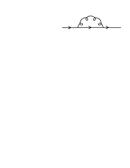
Figure  1.: Quark self energy having quark momentum $K$.

The most general ansatz for the fermionic self energy in rest frame of the plasma is given by  [?]

$$\Sigma(K)=-a(k_{0},k)K\!\!\!\!/\,-b(k_{0},k)\gamma_{0}\ ,$$ (27)

where $K=(k_{0},{\bf k})$, $k=|{\bf k}|$ and the quark mass is neglected assuming that the temperature is much larger than the quark mass, which holds at least for $u$ and $d$ quarks. The scalar quantities $a$ and $b$ are given by the traces over self energies within HTL approximations in figure 1 as, respectively,

$$a(k_{0},k) = \frac{1}{4k^{2}}\>\left[{\rm{tr}}\,(K\!\!\!\!/\,\Sigma)-k_{0}\>{\rm{tr}}\,(\gamma_{0}\Sigma)\right]=\frac{m_{q}^{2}}{k^{2}}\>\left(1-\frac{k_{0}}{2k}\>\ln\frac{k_{0}+k}{k_{0}-k}\right)\ \ ,$$ (28)

$$b(k_{0},k) = \frac{1}{4k^{2}}\>\left[K^{2}\>{\rm{tr}}\,(\gamma_{0}\Sigma)-k_{0}\>{\rm{tr}}\,(K\!\!\!\!/\,\Sigma)\right]=\frac{m_{q}^{2}}{k^{2}}\>\left(-k_{0}+\frac{k_{0}^{2}-k^{2}}{2k}\>\ln\frac{k_{0}+k}{k_{0}-k}\right),$$ (29)

where $m_{q}^{2}={g^{2}T^{2}}/{6}$, is the effective quark mass. The quark self energy in (27) has an imaginary part below the light cone, $k_{0}^{2}-k^{2}<0$, representing Landau damping (LD) for space like quark momenta. Furthermore, the general ansatz in (27) is also chirally invariant in spite of the appearance of an effective quark mass.

3.3 Effective propagators and vertices in HTL-approximation

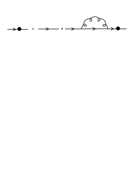
Figure  2.: Effective quark propagator in HTL-approximation

Resumming the quark self-energy by using the Dyson-Schwinger equation, the effective quark propagator in figure 2 can be written as

$$S(K)=[K\!\!\!\!/\,-\Sigma(K)]^{-1}=\frac{\gamma_{0}-\hat{\bf k}\cdot{\vec{\gamma}}}{2D_{+}(K)}+\frac{\gamma_{0}+\hat{\bf k}\cdot{\vec{\gamma}}}{2D_{-}(K)}\ \ ,$$ (30)

for massless quarks with a decomposition into helicity eigenstates, where

$$D_{\pm}(k_{0},k)=(1+a(k_{0},k))\>(-k_{0}\pm k)+b(k_{0},k)\ \ \ .$$ (31)

Figure  3.: Quark dispersion relation in HTL-approximation along with the free ($\omega=k$) one.

The relevant QED like HTL-vertex is related to this propagator through the Ward identity  [?,?]

$$K_{\mu}\Gamma^{\mu}(K_{1},K_{2};K)=S^{-1}(K_{1})-S^{-1}(K_{2})\ \ .$$ (32)

Now, the zeros of $D_{\pm}(K)$ give the in-medium propagation or quasiparticle (QP) dispersion relation. As shown in figure 3 the upper curve $\omega_{+}(k)$ corresponds to the solution of $D_{+}(K)=0$, whereas the lower curve $\omega_{-}(k)$ represents the solution of $D_{-}(K)=0$. Both branches start from a common effective mass, $m_{q}$, obtained in the $k\rightarrow 0$ limit  [?]. The $\omega_{+}(k)$ branch describes the propagation of an ordinary quark with thermal mass, and the ratio of its chirality to helicity is $+1$. On the other hand, the $\omega_{-}(k)$ branch corresponds to the propagation of a quark mode with a negative chirality to helicity ratio. This branch represents the plasmino mode which is absent in the vacuum but appears as consequence of the medium due to the broken Lorentz invariance, and has a shallow minimum. This corresponds to a purely collective long wave-length mode, whose spectral strength decreases exponentially at high momenta. For high momenta, however, both branches approach the free dispersion relation.

The spectral representation  [?,?] of HTL propagator in (30) can now be written as

$$\rho_{\pm} = \frac{1}{\pi}{\rm{Im}}f_{\pm}(x+i\epsilon)={\mathrm{Pole}}(k_{0}^{2}>k^{2})+{\mathrm{Cut}}(k_{0}^{2}<k^{2})\,\,.$$ (33)

4. Thermal Hadronic Correlation Function

While lattice calculations of hadron properties in vacuum have reached quite satisfactory precision, little is known from such first principle calculations about basic hadronic properties in a thermal medium. We want to analyse  [?] its behaviour in the high temperature limit through the thermal correlation functions in terms of quark fields.

4.1 Definition

Meson correlators are constructed from meson currents $J_{M}(\tau,\vec{x})=\bar{q}(\tau,\vec{x})\Gamma_{M}q(\tau,\vec{x})$, where $\Gamma_{M}=1$, $\gamma_{5}$, $\gamma_{\mu}$, $\gamma_{\mu}\gamma_{5}$ for scalar, pseudo-scalar, vector and pseudo-vector channels, respectively. The thermal two-point functions in coordinate space, $G_{M}(\tau,\vec{x})$, are defined as

$$G_{M}(\tau,\vec{x}) = \langle J_{M}(\tau,\vec{x})J_{M}^{\dagger}(0,\vec{0})\rangle=T\sum_{n=-\infty}^{\infty}\int{{\rm d}^{3}p\over(2\pi)^{3}}\;{\rm e}^{-i(\omega_{n}\tau-\vec{p}\vec{x})}\;\chi_{M}(\omega_{n},\vec{p})~{}~{},$$ (34)

where $\tau\in[0,1/T]$, and the Fourier transformed correlation function $\chi_{M}(\omega_{n},\vec{p})$ is given at the discrete Matsubara modes, $\omega_{n}=2n\pi T$. The imaginary part of the momentum space correlator gives the spectral function $\sigma_{M}(\omega,\vec{p})$,

$$\chi_{M}(\omega_{n},\vec{p})=-\int_{-\infty}^{\infty}{\rm d}\omega{\sigma_{M}(\omega,\vec{p})\over i\omega_{n}-\omega+i\epsilon}\Rightarrow\sigma_{M}(\omega,\vec{p})={1\over\pi}{\rm Im}\;\chi_{M}(\omega,\vec{p}).$$ (35)

Using (34) and (35) we obtain the spectral representation of the thermal correlation function in coordinate space at fixed momentum ($\beta=1/T$),

$$G_{M}(\tau,\vec{p})=\int_{0}^{\infty}{\rm d}\omega\;\sigma_{M}(\omega,\vec{p})\;{{\rm cosh}(\omega(\tau-\beta/2))\over{\rm sinh}(\omega\beta/2)}~{}~{}.$$ (36)

4.2 Hadronic spectral and correlation function in HTL-approximation

Figure  4.: Self-energy diagram involving quarks loop in HTL-approximation.

The hadronic spectral functions, $\sigma_{M}(\omega,p)$ in (35), of the temporal correlators are proportional to the imaginary part of the quark loop diagram. The meson spectral function  [?], constructed from two quark propagators, will have pole-pole, pole-cut and cut-cut contributions, $\sigma_{M}(\omega)=\sigma^{\rm{pp}}(\omega)+\sigma^{\rm{pc}}(\omega)+\sigma^{\rm{cc}}(\omega)$. Free meson spectral functions are also obtained using bare propagators and vertices in figure 4 as  [?,?] $\sigma^{{\rm free}}_{M}\left(\omega\right)=\frac{N_{C}}{4\pi^{2}}\omega^{2}\tanh\left(\frac{\omega}{4T}\right)a_{M}$ where $a_{M}=(+)-1$ for (pseudo)scalar and $(-)+2$ for (pseudo)vector.

Figure  5.: (a) Pseudoscalar and (b) vector meson spectral functions in HTL approximation for $m_{q}/T=1$. The free one is represented by crosses.

In figure 5 we show the different contributions for pseudoscalar and vector mesons  [?] for $m_{q}/T=1$, i.e., $g=\sqrt{6}$. Generically the pole-pole term of the meson spectral function in HTL-approximation describes three physical processes: (1) the annihilation of collective quarks, (2) the annihilation of two plasminos, and (3) the transition from upper to lower branch. The transition process starts at zero energy and continues until the maximum difference $\omega=0.47\>m_{q}$ between the two branches at $k=1.18\>m_{q}$. At this point a Van Hove singularity is encountered due to a diverging density of states for the third process as noted above. The plasmino annihilation starts at $\omega=1.86\>m_{q}$ with another Van Hove singularity corresponding to the minimum of the plasmino branch at $k=0.41\>m_{q}$, where again the density of states diverges corresponding to second process. This contribution falls off rapidly due to the exponentially suppressed spectral strength of the plasmino mode for large energies, where only the first process, quark-antiquark annihilation starting at $\omega=2m_{q}$, contributes. For large energies this dominates and approaches the free results (crosses) for $\omega>>m_{q}$. The pole-cut and cut-cut contributions, which involve external gluons as can be seen by cutting the HTL quark self energy in figure 4, lead to a smooth contribution to the spectral function. The pole-pole and pole-cut contributions in both channels are of similar magnitude, while the cut-cut contribution at small $\omega$ vanishes in the pseudoscalar channel but diverges in the vector channel. This has its origin in the structure of HTL quark-meson vertex  [?,?], which is required for the vector channel containing a collinear singularity, whereas bare vertices are sufficient for the (pseudo)scalar channel. In a very recent calculation  [?] using next to leading order HTL approximation, the pseudoscalar spectral function is found to remain almost same as the leading order results.

4.3 Dilepton production rate in HTL-approximation

The static dilepton production rate (${\vec{p}}=0$)  [?] is related to the vector meson channel as

$$\sigma_{V}(\omega)=\frac{1}{\pi}{\rm{Im}}\ \chi_{V}(\omega)=\frac{18\pi^{2}N_{C}}{5\alpha^{2}}\left(e^{\beta\omega}-1\right)\omega^{2}\frac{dR}{d^{4}xd\omega d^{3}p}({\vec{p}}=0).$$ (37)

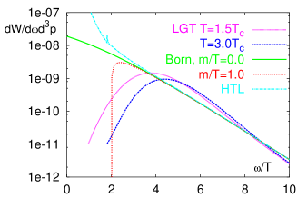
Figure  6.: The dilepton production rate in HTL-approximation for $m_{q}/T=2$ is compared with Lattice data.

In figure 6 we show the dilepton rates calculated from (37) in HTL and also in Born approximations, which are compared with the first dilepton rate obtained in lattice  [?]. The comparison of lattice rate with HTL and Born rate shows that for all energies $\omega/T\geq 4$ the difference is very small. For energies $\omega/T\leq 3$, the lattice dilepton rate drops rapidly and reflects sharp cut-off found in reconstructed spectral function  [?] and differs from that of HTL rate.

4.4 Meson correlation functions in HTL-approximation

Figure  7.: The pseudoscalar meson correlation functions in HTL-approximation (left) for $m_{q}/T=1$ and compared with lattice results.

The temporal correlators for pseudoscalar and vector mesons can be obtained from their spectral functions according to (36) in order to take into account of medium effects from the quark propagator. At larger temperatures it seems that the pseudoscalar correlator only slowly approaches the free correlation function and still differs from the lattice results  [?]. In other words, the HTL medium effects may not be sufficient to explain the deviation from free one. Details of the vector meson correlation function can be found in Ref.  [?].

5. Susceptibilities

Dynamical properties of a many particle system can be investigated by employing an external probe, which disturbs the system only slightly in its equilibrium state, and by measuring the response of the system to this external perturbation. Usually one probes the dynamical behavior of the spontaneous fluctuations in the equilibrium state. In general, spontaneous fluctuations are related to correlation functions. They reflect the symmetries of the system, which provide important inputs for quantitative calculations of complicated many-body systems. Recently, screening and fluctuations of conserved quantities have been proposed as a probe of the quark-gluon plasma (QGP) formation in ultrarelativistic heavy-ion collisions.

5.1 Definition

Let ${\cal O}_{\alpha}$ be a Heisenberg operator. In a static and uniform external field ${\cal F}_{\alpha}$, the (induced) expectation value of the operator ${\cal O}_{\alpha}\left(0,\overrightarrow{x}\right)$ is written as

$$\phi_{\alpha} \equiv \left\langle{\cal O}_{\alpha}\left(0,\overrightarrow{x}\right)\right\rangle_{F}=\frac{{\rm Tr}\left[{\cal O}_{\alpha}\left(0,\overrightarrow{x}\right)e^{-\beta\left({\cal H}+{\cal H}_{ex}\right)}\right]}{{\rm Tr}\left[e^{-\beta\left({\cal H}+{\cal H}_{ex}\right)}\right]}=\frac{1}{V}\int d^{3}x\,\left\langle{\cal O}_{\alpha}\left(0,\overrightarrow{x}\right)\right\rangle\>,$$ (38)

where the translational invariance is assumed and ${\cal H}_{ex}$ is given by ${\cal H}_{ex}=-\sum_{\alpha}\int d^{3}x\,{\cal O}_{\alpha}\left(0,\overrightarrow{x}\right){\cal F}_{\alpha}$ . The (static) susceptibility $\chi_{\alpha\beta}$ is defined as

$$\chi_{\alpha\sigma}(T) = \left.\frac{\partial\phi_{\alpha}}{\partial{\cal F}_{\sigma}}\right|_{{\cal F}=0}=\beta\int d^{3}x\,\left\langle{\cal O}_{\alpha}\left(0,\overrightarrow{x}\right){\cal O}_{\sigma}\left(0,\overrightarrow{0}\right)\right\rangle\>,$$ (39)

assuming no broken symmetry $\left\langle{\cal O}_{\alpha}\left(0,\overrightarrow{x}\right)\right\rangle=\left\langle{\cal O}_{\sigma}\left(0,\overrightarrow{0}\right)\right\rangle=0$. $\langle{\cal O}_{\alpha}(0,{\vec{x}}){\cal O}_{\sigma}(0,{\vec{0}})\rangle$ is the two point correlation function with operators evaluated at equal times.

5.2 Quark number susceptibility:

The quark number susceptibility is the measure of the response of the quark number density with infinitesimal changes in the quark chemical potential $\mu_{q}+\delta\mu_{q}$ and can be written as

$$\chi_{q}(T)=\left.\frac{\partial\rho_{q}}{\partial\mu_{q}}\right|_{\mu_{q}=0}=\beta\int\ d^{3}x\ \langle j_{0}(0,{\vec{x}})j_{0}(0,\vec{0})\rangle=\beta\int\ d^{3}x\ S_{00}(0,{\vec{x}})\,\,,$$ (40)

where $S_{00}(0,{\vec{x}})$ is the time-time component of vector meson correlator $S_{\mu\nu}(t,{\vec{x}})=\,\langle j_{\mu}(t,{\vec{x}})j_{\nu}(0,{\vec{0}})\rangle$. With the Fourier transform of $S_{00}(0,\vec{x})$ the (40) becomes

$$\chi_{q}\left(T\right) = \beta\int_{-\infty}^{+\infty}\frac{d\omega}{2\pi}\,S_{00}(\omega,0)\,\,\,\,{\rm{with}}\,\,\,S_{00}(\omega,p)=\frac{-2}{1-e^{-\beta\omega}}\,\rm{Im}\,\Pi_{00}\left(\omega,{\vec{p}}\right).$$ (41)

Using the imaginary part of the 1-loop vector meson self-energy within the HTL-approximation given in figure 8 the quark number susceptibility  [?] is computed through (41). It is found to contain  [?] only the quasiparticle (QP) contributions following from the QP dispersion relation $D_{\pm}=0$, given in (31). Note that the transversality condition in figure 8 eliminates the Landau damping (LD) contributions originating from the space like region.

Figure  8.: The 1-loop vector meson self energy diagram.

Figure  9.: The quark number susceptibility in HTL approximation scaled with free susceptibility is plotted as a function of $T/T_{C}$ with $T_{C}/\Lambda_{\bar{MS}}=0.69$. In each band the lower curve corresponds to the choice of the renormalization scale ${\bar{\mu}}=2\pi T$ and the upper one to ${\bar{\mu}}=2\pi T$. The squares represent recent lattice data.

The quark number susceptibility is plotted in figure 9 and compared with the lattice results. The result (band between the solid line denoted by QP) agrees well with recent lattice data  [?]. (Here we used the 2-loop result for the running coupling constant $g(T)$. For the renormalization scale $\bar{\mu}$ entering the running coupling constant, we choose two different values leading to the bands.) However, it overcounts the leading order perturbative result (dotted band denoted by PLO) given as $\chi_{q}/\chi_{f}=(1-2\alpha_{s}/\pi+\cdots)$. We note that this can be cured by going to the calculation at 2-loop order. Recently, it has been shown that the 2-loop order calculation  [?] for the thermodynamic potential reveals the correct inclusion of the leading order effects but happens to be very close to the 1-loop result. Now, employing only resummed propagators and bare vertices, the QNS contains LD contributions coming from the discontinuity of the 2-point HTL function in addition to the QP contribution. The result is shown in figure 9 by QP+LD. There are also calculations for quark number susceptibility within the approximately self-consistent HTL approximations  [?].

5.3 Chiral susceptibility

The chiral susceptibility measures the response of the chiral condensate to the infinitesimal change of the current quark mass $m+\partial m$. The static chiral susceptibility can be obtained as

$$\chi_{c}(T)=-\left.\frac{\partial\langle{\bar{q}}q\rangle}{\partial m}\right|_{m=0} = \beta\int{\rm d}^{3}x\;S(0,{\vec{x}})=\beta\int_{-\infty}^{+\infty}\frac{{\rm d}\omega}{2\pi}S(\omega,0)\,,$$ (42)

where $S(\omega,0)$ is the Fourier transformed correlator of the scalar channel.

Note that, in contrast to the quark number susceptibility  [?] where the zero temperature contribution vanishes due to the transversality properties of the vector channel, the static chiral susceptibility contains a quadratic ultraviolet divergence coming from the zero temperature contribution. Using dimensional regularization the temperature independent term disappears, as there is no scale associated with it, leading to $\chi_{c}^{f}(T)=-\frac{N_{f}N_{c}}{6}\>T^{2}$, where $N_{f}$ is the number of two light quark flavours and $N_{C}$ is the number of colour. The next order contribution follows from the two-loop thermodynamic potential given in Ref.  [?]. However, the second derivative of this expression with respect to $m$ diverges at $m=0$. Hence, the static chiral susceptibility cannot be calculated consistently in usual perturbation theory beyond leading order, but requires HTL resummation  [?].

Figure  10.: The 1-loop scalar meson tadpole diagram.

Now, we compute the chiral condensate $\langle q\bar{q}\rangle$ from the tadpole diagram in figure 10, where we use the effective HTL quark propagator, yielding  [?]

$$\frac{\chi_{c}^{h}(T)}{\chi_{c}^{f}(T)} = \left[1-\frac{6}{\pi^{2}}\left(\log\frac{\mu}{4\pi T}-\gamma-2\log 2\right)\frac{m_{q}^{2}}{T^{2}}\right.\left.+\frac{21}{4}\frac{\zeta(3)}{\pi^{4}}\left(5+\frac{8}{7}\log 2-\frac{\pi^{2}}{6}\right)\frac{m_{q}^{4}}{T^{4}}\right]\,.$$ (43)

Note that the $m_{q}^{2}$ term is the first finite $\alpha_{s}$ correction to the free chiral susceptibility, since the two-loop correction in usual perturbative QCD diverges for $m=0$. In figure 11, we show the chiral susceptibility in HTL approximation. In lattice simulations a peak around the critical temperature associated with chiral symmetry restoration has been observed. In contrast to lattice QCD the HTL approximation, although taking into account the medium effects in plasma due to the interactions, does not contain any physics related to the chiral restoration, which is truly a nonperturbative effect. However, we observe a strong increase of the magnitude of HTL chiral susceptibility towards low temperature similar as in lattice simulations above $T_{C}$.

Figure  11.: The HTL static susceptibility (free susceptibility subtracted) as a function of temperature for $\Lambda_{\overline{\rm{MS}}}=300$ MeV, and $N_{f}=2$ with the choices of the renormalization scale $\mu=2\pi T$ and $4\pi T$ for up to order $m_{q}^{2}$ (left) and up to order $m_{q}^{4}$ (right).

6. Dynamical Screening

Screening of charges in a plasma is one of the most important collective effects in plasma physics. In the classical limit in an isotropic and homogeneous plasma the screening potential of a point-like test charge $Q$ at rest can be derived from the linearized Poisson equation, resulting in Debye screening. Earlier in most calculations of the screening potential in the QGP, the test charge was assumed to be at rest. However, quarks and gluons coming from initial hard processes receive a transverse momentum which causes them to propagate through the QGP. In addition, hydrodynamical models predict a radial outward flow in the fireball. Hence, it is of great interest to estimate the screening potential of a parton moving  [?] relatively to the QGP. Chu and Matsui  [?] have used the Vlasov equation to investigate dynamic Debye screening for a heavy quark-antiquark pair traversing a quark-gluon plasma. They found that the screening potential becomes strongly anisotropic.

The screening potential of a moving charge $Q$ with velocity $v$ follows from the linearized Vlasov and Poisson equations as

$$\phi({\vec{r}},t;{\vec{v}})=\frac{Q}{2\pi^{2}}\int d^{3}k\frac{\exp{[-i{\vec{k}}\cdot({\vec{r}}-{\vec{v}}t)]}}{k^{2}{\rm Re}[\epsilon_{l}(\omega={\vec{k}}\cdot{\vec{v}},k)]}.$$ (44)

The dielectric function following from the semi-classical Vlasov equation describing a collisionless plasma is related to the high-temperature limit of the polarization tensor. For example, the longitudinal dielectric function following from the Vlasov equation is given by

$$\epsilon_{l}(\omega,k)=1-\frac{\Pi_{00}(\omega,k)}{k^{2}}=1+\frac{m_{D}^{2}}{k^{2}}\left(1-\frac{\omega}{2k}\ln\frac{\omega+k}{\omega-k}\right),$$ (45)

where the only non-classical inputs are Fermi and Bose distributions instead of the Boltzmann distribution. The gluon self-energies derived within the hard thermal loop approximation have been shown to be gauge invariant and the dielectric functions obtained from these are therefore also gauge invariant.

In the general case, for parton velocities $v$ between 0 and 1, we have to solve (44) together with (45) numerically. Since the potential is not isotropic anymore due to the velocity vector ${\vec{v}}$, we will restrict ourselves only to two cases, ${\vec{r}}$ parallel to ${\vec{v}}$ and ${\vec{r}}$ perpendicular to ${\vec{v}}$, i.e., for illustration we consider the screening potential only in the direction of the moving parton. The details of the perpendicular case can be found in Ref.  [?].

Figure  12.: Screening potential parallel to the velocity of the moving parton in a QGP.

In figure 12 the screening potential $\phi/Q$ in ${\vec{v}}$-direction is shown as a function of $r^{\prime}=r-vt$, where $r=|{\vec{r}}|$, between 0 and 6 fm for various velocities. For illustration we have chosen a strong fine structure constant $\alpha_{s}=g^{2}/(4\pi)=0.3$, a temperature $T=0.25$ GeV, and the number of quark flavors $N_{f}=2$. The shifted potentials  [?] depend only on $v$ and not on $t$ as it should be the case in a homogeneous and isotropic plasma. For $r^{\prime}<1$ fm one observes that the fall-off of the potential is stronger than for a parton at rest. The reason for this behavior is the fact that there is a stronger screening in the direction of the moving parton due to an enhancement of the particle density in the rest frame of the moving parton.

In addition, a minimum in the screening potential at $r^{\prime}>1$ fm shows up due to the loss of spherical symmetry of the Debye screening cloud. For example, for $v=0.8$ this minimum is at about 1.5 fm with a depth of about 8 MeV. A minimum in the screening potential is also known from non-relativistic, complex plasmas, where an attractive potential even between equal charges can be found if the finite extension of the charges is considered  [?]. A similar screening potential was found for a color charge at rest in Ref. [?], where a polarization tensor beyond the high-temperature limit was used. However, this approach has its limitation as a gauge dependent and incomplete (within the order of the coupling constant) approximation for the polarization tensor was used. Obviously, a minimum in the interparticle potential in a relativistic or non-relativistic plasma is a general feature if one goes beyond the Debye-Hückel approximation by either taking quantum effects, finite velocities, or finite sizes of the particles into account.

The modification of the confinement potential below the critical temperature into a Yukawa potential above the critical temperature might have important consequences for the discovery of the QGP in relativistic heavy-ion collisions. Bound states of heavy quarks, in particular the $J/\psi$ meson, which are produced in the initial hard scattering processes of the collision, will be dissociated in the QGP due to screening of the quark potential and break-up by energetic gluons. On the other hand, the formation of colored bound states, e.g., $qq$, $\bar{q}\bar{q}$, $gg$, of partons at rest has also been claimed  [?] above the critical temperature (2$T_{c}$ - 3$T_{c}$) by analyzing lattice data, indicating that the plasma behaves as a strongly coupled quark-gluon plasma. The dynamical screening will have important consequences on the $J/\Psi$ dissociation and other binary states formed in the QGP just above $T_{C}$.

7. Summary

In this lecture the thermal field theory within the imaginary time formalism has been introduced and some of the problems in computing physical quantities in bare perturbation theory are pointed out. In order to overcome these problems, the prescription of HTL resummation technique is discussed and based on it an improved perturbation theory (HTLpt) is also briefly outlined. Using this improved HTLpt various physical quantities, hadronic spectral and correlation functions, quark number and chiral susceptibilities, and the dynamical screening potentials have been computed and discussed at length.

REFERENCES

- [1] Proceeding of the 14th International Conference on Ultra-Relativistic Nucleus-Nucleus Collisions- Quark Matter’99”, Nucl. Phys A661 (2000).
- [2] Proceeding of the 17th International Conference on Ultra-Relativistic Nucleus-Nucleus Collisions- Quark Matter’04”, J. Phys. G30(2004).
- [3] F. Karsch, Lattice’99, Proceedings of the XVIIth International Symposium on Lattice Field Theory, Nucl. Phys. B (Proc. Suppl.) 83-84, 14c (2000).
- [4] J. I. Kapusta, Finite-Temperature Field Theory (Cambridge University Press, Cambridge, 1989).
- [5] M. Le Bellac, Thermal Field Theory (Cambridge University Press, Cambridge, 1996).
- [6] A.Das, Finite Temperature Field Theory (World Scientific, Singapore, 1997) p. 102.
- [7] M.H. Thoma, in Quark-Gluon Plasma 2, ed.: R.C. Hwa (World Scientific, Singapore, 1995) p.51; M. H. Thoma, New Developments and Application of Thermal Field Theory, hep-ph/0010164 .
- [8] K. Kajantie and J. I. Kapusta, Ann. Phys. (N.Y.) 160 (1985) 477.
- [9] J. C. Parikh, P. J. Siemens, and J.A. Lopez, Pramana 32 (1989) 555.
- [10] E. Braaten and R.D. Pisarski, Nucl. Phys. B 337 (1990) 569.
- [11] J. Frenkel and J. C. Taylor, Nucl. Phys. B 334 (1990) 199.
- [12] E. Braaten and R. D. Pisarski, Phys. Rev. D45 (1992) R1827.
- [13] J. O. Andersen, E. Braaten, and M. Strickland, Phys. Rev. Lett. 83 (1999) 2139.
- [14] F. Karsch, A. Patkós, and P. Petreczky, Phys. Lett. B401 (1997).
- [15] J. O. Andersen, E. Braaten, and M. Strickland, Phys. Rev. D 61 (2000) 014017.
- [16] J. O. Andersen, E. Braaten, and M. Strickland, Phys. Rev. D 61 (2000) 074016.
- [17] J. O. Andersen and M. Strickland, Phys. Rev. D 66 (2002) 105001.
- [18] J. O. Andersen, E. Braaten, E. Petitgirard and M. Strickland, Phys. Rev. D66 (2002) 085016; J. O. Andersen, E. Petitgirard and M. Strickland, Phys. Rev. D70 (2004) 045001.
- [19] E. Braaten, R.D. Pisarski, and T.C. Yuan, Phys. Rev. Lett. 64, (1990) 2242.
- [20] H.A. Weldon, Phys. Rev. D 26 (1982) 2789.
- [21] F. Karsch, M. G. Mustafa, and M.H. Thoma, Phys. Lett. B 497 (2001) 249.
- [22] W. Florkowski and B.L. Friman, Z. Phys. A 347 (1994) 271.
- [23] W. M. Alberico, A. Beraudo and A. Molinari, Nucl. Phys. A 750 (2005) 359.
- [24] F. Karsch et al, Phys. Lett. B 530 (2002) 147.
- [25] P. Chakraborty, M. G. Mustafa, Euro. Phys. Jour. C 23 (2002) 591; Phys. Rev. D 68 (2003) 085012.
- [26] R. V. Gavai and S. Gupta, Phys. Rev. D 65 (2002) 094515; R. V. Gavai, S. Gupta, and P. Phys. Rev. D 65 (2002) 054506.
- [27] J.-P. Blaizot, E. Iancu and A. Rebhan, Phys. Lett. B 523 (2001) 143; Euro. Phys. Jour. C 27 (2003) 433.
- [28] P. Chakraborty, M. G. Mustafa and M. H. Thoma, Phys. Rev. D 67 (2003) 114004.
- [29] M. G. Mustafa, M. H. Thoma and P. Chakraborty, Phys. Rev. C 71 (2005) 017901.
- [30] M. C. Chu and T. Matsui, Phys. Rev. D 39 (1989) 1892.
- [31] V. N. Tsytovich, JETP Lett. 78 (2003) 1283.
- [32] C. Gale and J. Kapusta, Phys. Lett. B 198 (1987) 89.
- [33] E V Shuryak and I Zahed, Phys. Rev D70 (2004) 054507.