Full $\cal{O}(\alpha)$ corrections to $e^{+}e^{-}\rightarrow\tilde{f}_{i}\ {\bar{\!\!\tilde{f}}}_{\!j}$

Abstract

We present a complete precision analysis of the sfermion pair production process $e^{+}e^{-}\rightarrow\tilde{f}_{i}\ {\bar{\!\!\tilde{f}}}_{\!j}\;(f=t,b,\tau,\nu_{\tau})$ in the Minimal Supersymmetric Standard Model. Our results extend the previously calculated weak corrections by including all one-loop corrections together with higher order QED corrections. We present the details of the analytical calculation and discuss the renormalization scheme. The numerical analysis shows the results for total cross-sections, forward-backward and left-right asymmetries. It is based on the SPS1a’ point from the SPA project. The complete corrections are about 10% and have to be taken into account in a high precision analysis.

I Introduction

The Minimal Supersymmetric Standard Model (MSSM) provides the most attractive extension of the Standard Model (SM). Among other particles it includes supersymmetric partners of the fermions. These scalar states ${\tilde{f}}_{L}$, ${\tilde{f}}_{R}$ (sfermions) correspond to the two chirality states of each fermion $f$. The mass eigenstates ${\tilde{f}}_{1}$ and ${\tilde{f}}_{2}$ though are not identical with ${\tilde{f}}_{L}$, ${\tilde{f}}_{R}$ and are rather a linear combination of them. The mixing terms are proportional to the mass of the corresponding fermion. Hence the sfermions of the third generation play a special r$\hat{\rm o}$le. As a consequence, one eigenstate (${\tilde{f}}_{1}$) can be much lighter than the other one.
The sfermions, especially the strongly interacting ones (${\tilde{t}}_{i},{\tilde{b}}_{i}$), are likely to be detected at the LHC or the Tevatron. Nevertheless, to extract the fundamental parameters one must have a significant accuracy only obtainable at a linear collider. From sfermion pair production in $e^{+}e^{-}$ collisions the sfermion mixing angle can be extracted. This is one of the reasons why it has been extensively studied phenomenologically exp . To match the expected precision of the linear collider, theory predictions must reach a similar accuracy. The effort to calculate higher order corrections to the sfermion production has begun by calculating the leading QCD, SUSY-QCD and Yukawa corrections QCD1 ; SUSY-QCD-A ; SUSY-QCD-H ; Yukawa . It was further shown that taking only the leading terms of the one-loop corrections is not sufficient and so also the full weak corrections were presented in letter ; hollik .
It is the aim of this paper to extend the existing weak corrections by including the full $\cal{O}(\alpha)$ contributions in a similar manner as in the case of the selectrons and the smuons in freitas . In addition, we present the full analytical results and all the details of the calculation for both the weak corrections letter and the QED contributions. Moreover, we generalize the results to include also the effects of polarization of the electron and positron beams. Apart from cross-sections, we calculate other observables such as the forward-backward and the left-right asymmetries as well.
Although we present the results in the form of cross-sections and asymmetries, we are well aware of the fact that the precise predictions have to be used for parameter extraction. As the definition of the parameters is no longer unique beyond the tree-level, there has been a recent proposal by the so-called SPA project (SUSY parameter analysis) which defines these parameters SPA . The SPA project also gives a firm base for calculating all sorts of observables (masses, decay widths, cross-sections etc.) and enables the development of tools for extracting the parameters.
The fundamental SUSY parameters in the SPA project are defined using the $\overline{\rm DR}$ (dimensional reduction) renormalization scheme at the scale $Q=1{\rm TeV}$. Specifying the renormalization scheme serves only to define the parameters uniquely and does not restrict the use of other schemes in different calculations. In this paper, we use an on-shell renormalization scheme. To use the parameters from the SPA project we have to translate them into the on-shell renormalization scheme. The results for any observable using different schemes (with correctly translated input parameters) must agree up to contributions of higher order.
The paper is organized as follows. In section II we give the formulae for the tree-level cross-section for polarized electron and positron beams. The calculation of the virtual corrections with a detailed discussion of the applied on-shell renormalization scheme are outlined in section III. All explicit analytic formulas needed for the calculation are given in the Appendices A, B, C and D. In section IV we work out the real radiative corrections where we include the Bremsstrahlung process $\sigma(e^{+}e^{-}\rightarrow\tilde{f}_{i}\ {\bar{\!\!\tilde{f}}}_{\!j}\gamma)$. In section V we present the numerical analysis with some results of the corrections. Section VI summarizes our conclusions.

II Tree level

The sfermion mixing is described by the diagonalization of the sfermion mass matrix given in the left-right basis $({\tilde{f}_{L}},{\tilde{f}_{R}})$ into the mass basis $({\tilde{f}}_{1},{\tilde{f}}_{2})$, $f=t,b$ or $\tau$ GunionHaber ,

$${\cal M}_{{\tilde{f}}}^{\,2} = \left(\begin{array}[]{cc}m_{{\tilde{f}}_{L}}^{\,2}&a_{f}\,m_{f}\\ a_{f}\,m_{f}&m_{{\tilde{f}}_{R}}^{\,2}\end{array}\right)=\left(R^{\tilde{f}}\right)^{\dagger}\left(\begin{array}[]{cc}m_{{\tilde{f}}_{1}}^{\,2}&0\\ 0&m_{{\tilde{f}}_{2}}^{\,2}\end{array}\right)R^{\tilde{f}}\,,$$ (5)

where $R^{\tilde{f}}_{i\alpha}$ is a 2 x 2 rotation matrix with rotation angle $\theta_{{\tilde{f}}}$, which relates the mass eigenstates ${\tilde{f}}_{i}$, $i=1,2$, $(m_{{\tilde{f}}_{1}}<m_{{\tilde{f}}_{2}})$ to the weak eigenstates ${\tilde{f}}_{\alpha}$, $\alpha=L,R$, by ${\tilde{f}}_{i}=R^{\tilde{f}}_{i\alpha}{\tilde{f}}_{\alpha}$, with $R^{\tilde{f}}_{11}=R^{\tilde{f}}_{22}=\cos\theta_{\tilde{f}}$ and $R^{\tilde{f}}_{12}=-R^{\tilde{f}}_{21}=\sin\theta_{\tilde{f}}$, and

$$m_{{\tilde{f}}_{L}}^{\,2} = M_{\{\tilde{Q},\,\tilde{L}\}}^{2}+(I^{3L}_{f}\!-\!e_{f}\,s_{W}^{2})\cos 2\beta\,m_{Z}^{\,2}+m_{f}^{2}\,,$$ (6)

$$m_{{\tilde{f}}_{R}}^{\,2} = M_{\{\tilde{U},\,\tilde{D},\,\tilde{E}\}}^{2}+e_{f}\,s_{W}^{2}\cos 2\beta\,m_{Z}^{\,2}+m_{f}^{2}\,,$$ (7)

$$a_{f} = A_{f}-\mu\,(\tan\beta)^{-2I^{3L}_{f}}\,.$$ (8)

$M_{\tilde{Q}}$, $M_{\tilde{L}}$, $M_{\tilde{U}}$, $M_{\tilde{D}}$ and $M_{\tilde{E}}$ are soft SUSY breaking masses, $A_{f}$ is the trilinear scalar coupling parameter, $\mu$ the higgsino mass parameter, $\tan\beta=\frac{v_{2}}{v_{1}}$ is the ratio of the vacuum expectation values of the two neutral Higgs doublet states , $I^{3L}_{f}$ denotes the third component of the weak isospin of the fermion $f$, $e_{f}$ the electric charge in terms of the elementary charge $e$, and $s_{W}$ is the sine of the Weinberg angle $\theta_{W}$.
The mass eigenvalues and the mixing angle are

$$m_{\tilde{f}_{1,2}}^{2} = \frac{1}{2}\left(m_{\tilde{f}_{L}}^{2}+m_{\tilde{f}_{R}}^{2}\mp\sqrt{(m_{\tilde{f}_{L}}^{2}\!-\!m_{\tilde{f}_{R}}^{2})^{2}+4a_{f}^{2}m_{f}^{2}}\,\right)\,,$$ (9)

$$\cos\theta_{{\tilde{f}}} = \frac{-a_{f}\,m_{f}}{\sqrt{(m_{\tilde{f}_{L}}^{2}\!-\!m_{\tilde{f}_{1}}^{2})^{2}+a_{f}^{2}m_{f}^{2}}}\hskip 56.9055pt(0\leq\theta_{{\tilde{f}}}<\pi)\,,$$ (10)

and the mass of the sneutrino $\tilde{\nu}_{\tau}$ is given by $m_{\tilde{\nu}_{\tau}}^{2}=M_{\tilde{L}}^{2}+\frac{1}{2}\,m_{Z}^{2}\cos 2\beta$.

The tree-level cross-section of $e^{+}e^{-}\rightarrow\tilde{f}_{i}\ {\bar{\!\!\tilde{f}}}_{\!j}$ for polarized electron and positron beams is given by

$$\sigma^{\rm tree} = \frac{1}{4}(1-P_{-})(1+P_{+})\,\sigma_{L}^{\rm tree}+\frac{1}{4}(1+P_{-})(1-P_{+})\,\sigma_{R}^{\rm tree}\,,$$ (11)

where $P_{-},P_{+}\in(-1,1)$ are the degrees of polarization of the electron and positron beams (e. g. $P_{-}(P_{+})=-0.8$ means 80% of electrons (positrons) left polarized and 20 % unpolarized).

As we neglect the electron mass, we have only two terms contributing (out of 4 possible) where $\sigma_{L}^{\rm tree}$ is the tree-level cross-sections for $e_{R}^{+}\,e_{L}^{-}\rightarrow\tilde{f}_{i}\ {\bar{\!\!\tilde{f}}}_{\!j}$ (below referred to as the left part of the polarized cross-section) and $\sigma_{R}^{\rm tree}$ stands for $e_{L}^{+}e_{R}^{-}\rightarrow\tilde{f}_{i}\ {\bar{\!\!\tilde{f}}}_{\!j}$ (analogously referred to as the right part of the cross-section). They have the form

$$\sigma_{L,R}^{\rm tree}(e^{+}e^{-}\rightarrow\tilde{f}_{i}\ {\bar{\!\!\tilde{f}}}_{\!j}) = \frac{N_{C}}{3}\frac{\kappa^{3}(s,m^{2}_{{\tilde{f}}_{i}},m^{2}_{{\tilde{f}}_{j}})}{4\,\pi\,s^{2}}\left(T_{L,R}^{\gamma\gamma}+T_{L,R}^{\gamma Z}+T_{L,R}^{ZZ}\right)\,,$$ (12)

where

$$T_{L,R}^{\gamma\gamma} = \frac{e^{4}e_{f}^{2}(\delta_{ij})^{2}}{s^{2}}{\displaystyle\frac{1}{2}}K_{L,R}^{2}\,,$$ (13)

$$T_{L,R}^{\gamma Z} = -\frac{g_{Z}^{2}e^{2}e_{f}a_{ij}^{\tilde{f}}\delta_{ij}}{4s(s-m_{Z}^{2})}\,C_{L,R}K_{L,R}\,,$$ (14)

$$T_{L,R}^{ZZ} = \frac{g_{Z}^{4}(a_{ij}^{\tilde{f}})^{2}}{32\,(s-m_{Z}^{2})^{2}}\,C_{L,R}^{2}\,,$$ (15)

and $\kappa(x,y,z)=\sqrt{(x-y-z)^{2}-4yz}$.
Here we use $K_{L,R}$ and $C_{L,R}$ as the left- and right-handed couplings of the electron to the photon and $Z$-boson, respectively,

$$K_{L}=K_{R}=1,\qquad C_{L}=-\frac{1}{2}+s_{W}^{2},\qquad C_{R}=s_{W}^{2}.$$ (16)

The matrix elements $a_{ij}^{\tilde{f}}$ come from the coupling of $Z{\tilde{f}}_{i}{\tilde{f}}_{j}$,

$$a_{ij}^{\tilde{f}} = \left(\begin{array}[]{cc}4(I^{3L}_{f}\cos^{2}\theta_{\tilde{f}}-s_{W}^{2}e_{f})&-2I^{3L}_{f}\sin 2\theta_{\tilde{f}}\\ -2I^{3L}_{f}\sin 2\theta_{\tilde{f}}&4(I^{3L}_{f}\cos^{2}\theta_{\tilde{f}}-s_{W}^{2}e_{f})\end{array}\right).$$ (19)

Apart from the tree-level cross-section we can calculate other observables such as the left-right asymmetry and the forward-backward asymmetry. They are defined by

$$A_{LR}\,=\,\frac{\sigma_{L}-\sigma_{R}}{\sigma_{L}+\sigma_{R}}\,,\qquad\quad A_{FB}\,=\,\frac{\sigma_{F}-\sigma_{B}}{\sigma_{F}+\sigma_{B}}\,,$$ (20)

with

$$\sigma_{F}\,=\,\int_{0}^{2\pi}d\varphi\int_{0}^{\pi/2}\left(\frac{d\sigma}{d\Omega}\right)\,d\cos\vartheta\,,\qquad\quad\sigma_{B}\,=\,\int_{0}^{2\pi}d\varphi\int_{\pi/2}^{\pi}\left(\frac{d\sigma}{d\Omega}\right)\,d\cos\vartheta\,.$$ (21)

There is no lowest order (tree-level) contribution to the $A_{FB}$-asymmetry as the angle distribution is symmetric.

III Virtual corrections

For a precision analysis of the sfermion production one has to include also higher order corrections. The calculation of the higher order corrections is performed analytically in the $\overline{\rm DR}$ scheme, adopting the $\xi=1$ ’tHooft-Feynman gauge. All necessary ingredients of the analytical calculation are given in the Appendices. Furthermore, we neglect the electron mass wherever possible $(m_{e}=0)$. For the numerical evaluation of the loop integrals we use the packages LoopTools and FF loopFF . At the end the whole analytic result was checked with the result obtained using the computer algebra tools FeynArts and FormCalc feyn .
The virtual corrections receive contributions from vertex, self-energy and box diagrams depicted generically in Fig. 1 and explicitly in Figs. 2 and 3. All these contributions are summarized in the renormalized cross-section $\sigma^{\rm ren}$.
The one-loop (renormalized) cross-section $\sigma^{\rm ren}$ for polarized beams is expressed analogously to Eq. (11),

$$\sigma^{\rm ren}(e^{+}e^{-}\rightarrow\tilde{f}_{i}\ {\bar{\!\!\tilde{f}}}_{\!j}) = \frac{1}{4}(1-P_{-})(1+P_{+})\,\sigma_{L}^{\rm ren}+\frac{1}{4}(1+P_{-})(1-P_{+})\,\sigma_{R}^{\rm ren}\,,$$ (22)

where the left/right renormalized cross-sections are defined as

$$\sigma^{\rm ren}_{L,R} = \sigma^{\rm tree}_{L,R}+\Delta\sigma^{\rm QCD}_{L,R}+\Delta\sigma^{\rm EW}_{L,R}$$ (23)

with the symbol $\Delta$ denoting UV-finite quantities.
The SUSY-QCD corrections ($\Delta\sigma^{\rm QCD}$) have already been calculated for the unpolarized case in SUSY-QCD-A ; SUSY-QCD-H . As the gluon part of $\Delta\sigma^{\rm QCD}$ is proportional to the tree-level cross-section, the polarized cross-sections are easily obtained using $\sigma^{tree}_{L,R}$ instead of $\sigma^{tree}$. The gluino part of $\Delta\sigma^{\rm QCD}$ is treated analogously to $\Delta\sigma^{V{\tilde{f}}}$ (see Fig. 1).

Figure 1: UV-finite parts of the electro-weak corrections

We have already presented the unpolarized results for the electro-weak corrections ($\Delta\sigma^{\rm EW}$) in letter . In this paper, we give the result for polarized beams and also all formulas needed for the calculation.
The electroweak corrections can be split further into four UV-finite parts given in Fig. 1,

$$\Delta\sigma^{\rm EW}_{L,R} = \Delta\sigma^{\rm V\hskip 1.0pte}_{L,R}+\Delta\sigma^{\rm V\hskip 1.0pt\tilde{f}}_{L,R}+\Delta\sigma^{\rm prop}_{L,R}+\Delta\sigma^{\rm box}_{L,R}\,,$$ (24)

where $\Delta\sigma^{\rm V\hskip 1.0pte}_{L,R}$ and $\Delta\sigma^{\rm V\hskip 1.0pt\tilde{f}}_{L,R}$ stand for the left/right part of the renormalized electron and sfermion vertex, $\Delta\sigma^{\rm prop}_{L,R}$ and $\Delta\sigma^{\rm box}_{L,R}$ for the left/right part of renormalized propagators and box contribution.
The renormalized electron vertex has the form

$$\Delta\sigma^{\rm V\hskip 1.0pte}_{L,R} = \frac{N_{C}}{3}\frac{\kappa^{3}(s,m^{2}_{{\tilde{f}}_{i}},m^{2}_{{\tilde{f}}_{j}})}{4\,\pi\,s^{2}}\left(\left(\Delta T^{V\hskip 1.0pte}_{\gamma\gamma}\right)_{L,R}+\left(\Delta T^{V\hskip 1.0pte}_{\gamma Z}\right)_{L,R}+\left(\Delta T^{V\hskip 1.0pte}_{ZZ}\right)_{L,R}\right),$$ (25)

where

$$\left(\Delta T^{V\hskip 1.0pte}_{\gamma\gamma}\right)_{L,R} = \frac{e^{4}e_{f}^{2}(\delta_{ij})^{2}}{s^{2}}\,(\Delta e_{L,R}K_{L,R})\,,$$ (26)

$$\left(\Delta T^{V\hskip 1.0pte}_{\gamma Z}\right)_{L,R} = -\frac{g_{Z}^{2}e^{2}e_{f}a_{ij}^{\tilde{f}}\delta_{ij}}{4s(s-m_{Z}^{2})}\,(\Delta e_{L,R}C_{L,R}+\Delta a_{L,R}K_{L,R})\,,$$ (27)

$$\left(\Delta T^{V\hskip 1.0pte}_{ZZ}\right)_{L,R} = \frac{g_{Z}^{4}(a_{ij}^{\tilde{f}})^{2}}{16\,(s-m_{Z}^{2})^{2}}\,(\Delta a_{L,R}C_{L,R}).$$ (28)

$\Delta e_{L,R}$ and $\Delta a_{L,R}$ consist of 3 parts,

$$\Delta e_{L,R} = \delta e_{L,R}^{(v)}+\delta e_{L,R}^{(w)}+\delta e_{L,R}^{(c)}\,,$$ (29)

$$\Delta a_{L,R} = \delta a_{L,R}^{(v)}+\delta a_{L,R}^{(w)}+\delta a_{L,R}^{(c)}\,.$$ (30)

$\delta e_{L,R}^{(v)}$, $\delta a_{L,R}^{(v)}$ correspond to the vertex corrections in Fig. 2, $\delta e_{L,R}^{(w)}$, $\delta a_{L,R}^{(w)}$ are the wave-function corrections, and $\delta e_{L,R}^{(c)}$, $\delta a_{L,R}^{(c)}$ correspond to the counterterms.
The renormalized sfermion vertex has a similar form,

$$\Delta\sigma^{\rm V\hskip 1.0pt\tilde{f}}_{L,R} = \frac{N_{C}}{3}\frac{\kappa^{3}(s,m^{2}_{{\tilde{f}}_{i}},m^{2}_{{\tilde{f}}_{j}})}{4\,\pi\,s^{2}}\left(\left(\Delta T^{V\hskip 1.0pt\tilde{f}}_{\gamma\gamma}\right)_{L,R}+\left(\Delta T^{V\hskip 1.0pt\tilde{f}}_{\gamma Z}\right)_{L,R}+\left(\Delta T^{V\hskip 1.0pt\tilde{f}}_{ZZ}\right)_{L,R}\right)\,,$$ (31)

where

$$\left(\Delta T^{V\hskip 1.0pt\tilde{f}}_{\gamma\gamma}\right)_{L,R} = \frac{e^{4}e_{f}(\Delta e_{f})_{ij}}{s^{2}}\,K_{L,R}^{2}\,,$$ (32)

$$\left(\Delta T^{V\hskip 1.0pt\tilde{f}}_{\gamma Z}\right)_{L,R} = -\frac{g_{Z}^{2}\,e^{2}}{4s(s-m_{Z}^{2})}\,K_{L,R}C_{L,R}\,((\Delta e_{f})_{ij}a_{ij}^{\tilde{f}}+\delta_{ij}(\Delta a_{f})_{ij})\,,$$ (33)

$$\left(\Delta T^{V\hskip 1.0pt\tilde{f}}_{ZZ}\right)_{L,R} = \frac{g_{Z}^{4}\,a_{ij}^{\tilde{f}}(\Delta a_{f})_{ij}}{16\,(s-m_{Z}^{2})^{2}}\,C_{L,R}^{2}\,.$$ (34)

$(\Delta e_{f})_{ij}$ and $(\Delta a_{f})_{ij}$ can also be split into vertex corrections (see Fig. 2), wave-function corrections and counterterms,

$$(\Delta e_{f})_{ij} = (\delta e_{f})_{ij}^{(v)}+(\delta e_{f})_{ij}^{(w)}+(\delta e_{f})_{ij}^{(c)}\,,$$ (35)

$$(\Delta a_{f})_{ij} = (\delta a_{f})_{ij}^{(v)}+(\delta a_{f})_{ij}^{(w)}+(\delta a_{f})_{ij}^{(c)}\,.$$ (36)

The diagrams contributing to the vertex corrections are shown in Fig. 2 and the explicit form of the corrections are given in Appendix A. The wave-function corrections and the counterterms to both vertices are listed in detail in sections III.1.1 and III.1.2. The $(\delta e_{f})_{ij}$ and $(\delta a_{f})_{ij}$ corresponding to gluino corrections can be found in SUSY-QCD-H .

Figure 2: Vertex diagrams contributing to $\delta e_{L,R}^{(v)}$ , $\delta a_{L,R}^{(v)}$ , $(\delta e_{f})_{ij}^{(v)}$ and $(\delta a_{f})_{ij}^{(v)}$.

The correction $\Delta\sigma^{\rm prop}_{L,R}$ which comes from inserting the self-energies of the $\gamma$ and $Z$-boson, in the propagator, see Fig. 3, can be expressed as

$$\Delta\sigma^{\rm prop}_{L,R} = \frac{N_{C}}{3}\frac{\kappa^{3}(s,m^{2}_{{\tilde{f}}_{i}},m^{2}_{{\tilde{f}}_{j}})}{4\,\pi\,s^{2}}\times$$

$$\times\,2\,\Re\left[\left(-\frac{{\hat{\Pi}_{\gamma\gamma}^{T}(s)}}{s}\right)\,T^{\gamma\gamma}_{L,R}+\left(-\frac{{\hat{\Pi}_{\gamma\gamma}^{T}(s)}}{s}-\frac{{\hat{\Pi}_{ZZ}^{T}(s)}}{s-m_{Z}^{2}}\right)\,T^{\gamma Z}_{L,R}+\left(-\frac{{\hat{\Pi}_{ZZ}^{T}(s)}}{s-m_{Z}^{2}}\right)\,T^{ZZ}_{L,R}\right.$$

$$\left.+\left(s_{W}c_{W}\frac{{\hat{\Pi}_{Z\gamma}^{T}(s)}}{s}\right)\,\left((T_{Z\gamma}^{\gamma})_{L,R}+(T_{ZZ}^{\gamma})_{L,R}\right)+\left(\frac{1}{s_{W}c_{W}}\frac{{\hat{\Pi}_{\gamma Z}^{T}(s)}}{s-m_{Z}^{2}}\right)\,\left((T_{\gamma\gamma}^{Z})_{L,R}+(T_{\gamma Z}^{Z})_{L,R}\right)\right]\,,$$

where $T^{\gamma\gamma}_{L,R}$, $T^{\gamma Z}_{L,R}$, $T^{ZZ}_{L,R}$ are defined in Eqs. (13-15) and

$$(T_{Z\gamma}^{\gamma})_{L,R} = -\frac{g_{Z}^{2}e^{2}e_{f}a_{ij}^{\tilde{f}}\delta_{ij}}{4s\,(s-m_{Z}^{2})}\,{\displaystyle\frac{1}{2}}K_{L,R}^{2}\,,$$ (38)

$$(T_{ZZ}^{\gamma})_{L,R} = \frac{g_{Z}^{4}(a_{ij}^{\tilde{f}})^{2}}{16\,(s-m_{Z}^{2})^{2}}\,{\displaystyle\frac{1}{2}}C_{L,R}K_{L,R}\,,$$ (39)

$$(T_{\gamma\gamma}^{Z})_{L,R} = \frac{e^{4}e_{f}^{2}(\delta_{ij})^{2}}{s^{2}}{\displaystyle\frac{1}{2}}C_{L,R}K_{L,R}\,,$$ (40)

$$(T_{\gamma Z}^{Z})_{L,R} = -\frac{g_{Z}^{2}e^{2}e_{f}a_{ij}^{\tilde{f}}\delta_{ij}}{4s\,(s-m_{Z}^{2})}\,{\displaystyle\frac{1}{2}}C_{L,R}^{2}\,.$$ (41)

The ${\hat{\Pi}_{VV}^{T}(s)}$ in Eq. (III) are the transverse parts of the renormalized self-energies of the vector bosons $\gamma$ and $Z$. The unrenormalized self-energies are given in Appendix C.2 and the renormalization is done following Denner .
The box corrections are obtained by adding up the diagrams shown in Fig. 3 and are given by

$$\Delta\sigma^{\rm box}_{L,R} = \frac{N_{C}}{4}\,\frac{\kappa^{3}(s,m^{2}_{{\tilde{f}}_{i}},m^{2}_{{\tilde{f}}_{j}})}{4\,\pi\,s^{2}}\!{\displaystyle{\int_{0}^{\pi}}}\!T_{L,R}^{\rm box}\,\sin^{2}\vartheta\;{\rm d}\vartheta\,,$$ (42)

where

$$T_{L,R}^{\rm box} = \left(-\frac{1}{(4\pi)^{2}}\frac{e^{2}e_{f}\delta_{ij}}{s}\frac{1}{2}K_{L,R}+\frac{1}{(4\pi)^{2}}\frac{g_{Z}^{2}\,a^{\tilde{f}}_{ij}}{4(s-m_{Z}^{2})}\frac{1}{2}C_{L,R}\right)\,B_{L,R}\,.$$ (43)

The $B_{L,R}$ are the form-factors defined in Appendix B, where one can find the analytic expressions as well.

Figure 3: Diagrams contributing to the propagator and the box corrections.

III.1 Renormalization scheme

In order to make the result finite we have to introduce the wave-function renormalization constants and counterterms. We fix them following the on-shell renormalization scheme. The parameters already occurring in the Standard Model (SM) are renormalized according to Denner . We assume the CKM matrix to be diagonal and so have no flavour mixing among the SM fermions at one-loop level.

III.1.1 Wave-function renormalization

The wave-function corrections are due to a shift from unrenormalized (bare) fields to the renormalized (physical) ones. For the fields relevant here we have

$${\tilde{f}}_{i}^{0}=(\delta_{ij}+{\textstyle\frac{1}{2}}\delta Z_{ij}){\tilde{f}}_{j}\,,\qquad \left(\begin{array}[]{c}f_{L}^{0}\\ f_{R}^{0}\end{array}\right)=\left(\begin{array}[]{cc}1+{\textstyle\frac{1}{2}}\delta Z_{L}&0\\ 0&1+{\textstyle\frac{1}{2}}\delta Z_{R}\end{array}\right)\left(\begin{array}[]{c}f_{L}\\ f_{R}\end{array}\right),$$ (50)

$$\left(\begin{array}[]{c}A_{\mu}^{0}\\ Z_{\mu}^{0}\end{array}\right) = \left(\begin{array}[]{cc}1+{\textstyle\frac{1}{2}}\delta Z_{\gamma\gamma}&{\textstyle\frac{1}{2}}\delta Z_{\gamma Z}\\ {\textstyle\frac{1}{2}}\delta Z_{Z\gamma}&1+{\textstyle\frac{1}{2}}\delta Z_{ZZ}\end{array}\right)\left(\begin{array}[]{c}A_{\mu}\\ Z_{\mu}\end{array}\right).$$ (57)

The form of the corrections for the left vertex is

$$\delta e_{L,R}^{(w)} = (\delta Z_{L,R}+{\textstyle\frac{1}{2}}\delta Z_{\gamma\gamma})K_{L,R}-{\displaystyle\frac{1}{2}}\frac{g_{Z}}{e}\delta Z_{Z\gamma}C_{L,R}\,,$$ (58)

$$\delta a_{L,R}^{(w)} = (\delta Z_{L,R}+{\textstyle\frac{1}{2}}\delta Z_{ZZ})C_{L,R}-{\displaystyle\frac{1}{2}}\frac{e}{g_{Z}}\delta Z_{\gamma Z}K_{L,R}\,.$$ (59)

The wave-function corrections for the right vertex are

$$(\delta e_{f})_{ij}^{(w)} = {\displaystyle\frac{1}{2}}e_{f}(\delta Z_{ij}+\delta Z_{ji})+{\displaystyle\frac{1}{2}}e_{f}\delta Z_{\gamma\gamma}\,\delta_{ij}+\frac{1}{8s_{W}c_{W}}a^{{\tilde{f}}}_{ij}\,\delta Z_{Z\gamma}\,,$$ (60)

$$(\delta a_{f})_{ij}^{(w)} = {\displaystyle\frac{1}{2}}\sum_{k=1}^{2}\left(\delta Z_{ki}\,a^{{\tilde{f}}}_{kj}+\delta Z_{kj}\,a^{{\tilde{f}}}_{ik}\right)+2s_{W}c_{W}e_{f}\,\delta_{ij}\,\delta Z_{\gamma Z}+{\displaystyle\frac{1}{2}}a^{{\tilde{f}}}_{ij}\,\delta Z_{ZZ}\,,$$ (61)

where $s_{W}=\sin\theta_{W}$ and $c_{W}=\cos\theta_{W}$.
The wave-function renormalization constants are determined by imposing the on-shell renormalization conditions as in onshellren ; sche2 such that the on-shell masses are the real parts of the poles of the propagator and the fields are properly normalized,

$$\delta Z_{ii} = -\Re\,\dot{\Pi}_{ii}^{{\tilde{f}}}(m_{{\tilde{f}}_{i}}^{2})\,,\qquad\delta Z_{ij}~{}=~{}\frac{2\,\Re\,\Pi_{ij}^{{\tilde{f}}}(m_{{\tilde{f}}_{j}}^{2})}{m_{\tilde{f}_{i}}^{2}-m_{\tilde{f}_{j}}^{2}}\,,\;\qquad\delta Z_{\gamma\gamma}~{}=~{}-\Re\,\dot{\Pi}_{\gamma\gamma}(0)\,,$$ (62)

$$\delta Z_{ZZ} = -\Re\,\dot{\Pi}_{ZZ}(m_{Z}^{2})\,,\;\quad\delta Z_{\gamma Z}~{}=~{}-\frac{2\,\Re\,\Pi_{\gamma Z}(m_{Z}^{2})}{m_{Z}^{2}}\,,\quad\delta Z_{Z\gamma}~{}=~{}\frac{2\,\Re\,\Pi_{Z\gamma}(0)}{m_{Z}^{2}}\,,$$ (63)

$$\delta Z_{L} = \Re\,\left[-\Pi_{L}(m_{e}^{2})-m_{e}^{2}(\dot{\Pi}_{L}(m_{e}^{2})+\dot{\Pi}_{R}(m_{e}^{2}))+\frac{1}{2m_{e}}(\Pi_{SL}(m_{e}^{2})-\Pi_{SR}(m_{e}^{2}))\right.$$ (64)

$$\left.-m_{e}(\dot{\Pi}_{SL}(m_{e}^{2})+\dot{\Pi}_{SR}(m_{e}^{2}))\right]\,,$$

$$\delta Z_{R} = \Re\,\left[-\Pi_{R}(m_{e}^{2})-m_{e}^{2}(\dot{\Pi}_{R}(m_{e}^{2})+\dot{\Pi}_{L}(m_{e}^{2}))+\frac{1}{2m_{e}}(\Pi_{SR}(m_{e}^{2})-\Pi_{SL}(m_{e}^{2}))\right.$$ (65)

$$\left.-m_{e}(\dot{\Pi}_{SR}(m_{e}^{2})+\dot{\Pi}_{SL}(m_{e}^{2}))\right]\,,$$

where $\dot{\Pi}(m^{2})=\left[\frac{\partial}{\partial k^{2}}\Pi(k^{2})\right]_{k^{2}=m^{2}}$. We use the self-energies given in Appendix C and in chrislet where we adopted the conventions from.
A remark should be made at this point. We include the wave-functions renormalization constants of the vector bosons although they are not external particles. By introducing them into the wave-function renormalization of the vertices, we have additional checks that can be made. First of all, the renormalization constants of the vector bosons must drop out in the final result. Secondly, the vertex corrections and the propagators can be both made UV-finite separately.

III.1.2 Counterterms

The counterterms come from the shift from the bare to the physical parameters in the lagrangian. It includes the shifting of $e,m_{W},m_{Z},\theta_{\tilde{f}}$ defined by

$$e^{0}=e+\delta e\,,\qquad m_{W}^{0}=m_{W}+\delta m_{W}\,,\qquad m_{Z}^{0}=m_{Z}+\delta m_{Z}\,,\qquad\theta_{\tilde{f}}^{0}=\theta_{\tilde{f}}+\delta\theta_{\tilde{f}}\,.$$ (66)

The counterterm contributions for both vertices are

$$\delta e_{L,R}^{(c)} = \frac{\delta e}{e}\,K_{L,R}\,,$$ (67)

$$\delta a_{L,R}^{(c)} = \left[\frac{\delta e}{e}-\left(\frac{\delta m_{W}}{m_{W}}-\frac{\delta m_{Z}}{m_{Z}}\right)+\frac{1-2s_{W}}{t_{W}^{2}}\left(\frac{\delta m_{W}}{m_{W}}-\frac{\delta m_{Z}}{m_{Z}}\right)\right]\,C_{L,R}\,,$$ (68)

$$(\delta e_{f})_{ij}^{(c)} = \frac{\delta e}{e}\,e_{f}\,\delta_{ij}\,,$$ (69)

$$(\delta a_{f})_{ij}^{(c)} = \left[\frac{\delta e}{e}+\frac{c_{W}^{2}-s_{W}^{2}}{s_{W}^{2}}\left(\frac{\delta m_{W}}{m_{W}}-\frac{\delta m_{Z}}{m_{Z}}\right)\right]\,a^{{\tilde{f}}}_{ij}+8e_{f}c_{W}^{2}\left(\frac{\delta m_{W}}{m_{W}}-\frac{\delta m_{Z}}{m_{Z}}\right)\,\delta_{ij}\,,$$ (70)

where the contributions containing $\delta\theta_{\tilde{f}}$ were intentionally left out and will be discussed below.

III.1.3 Renormalization of electric charge

The standard on-shell input value for the electric charge is the one in the Thomson limit $\alpha\equiv e^{2}/(4\pi)=1/137.036$. This corresponds to a counterterm

$$\frac{\delta e}{e} = \frac{1}{2}\,\delta Z_{\gamma\gamma}-\frac{s_{W}}{2c_{W}}\,\delta Z_{Z\gamma}\,.$$ (71)

In this way of fixing the electric charge has a significant theoretical uncertainty coming from the light quarks which we circumvent by using as input parameter for $\alpha$ the $\overline{\rm MS}$ value at the $Z$-pole, $\alpha\equiv\alpha(m_{Z})|_{\overline{\rm MS}}=e^{2}/(4\pi)$. The counterterm then is given by chrislet ; 0111303 ; wcharge

$$\frac{\delta e}{e} = \frac{1}{(4\pi)^{2}}\,\frac{e^{2}}{6}\Bigg{[}\,4\sum_{f}N_{C}^{f}\,e_{f}^{2}\bigg{(}\Delta+\log\frac{Q^{2}}{x_{f}^{2}}\bigg{)}+\sum_{{\tilde{f}}}\sum_{m=1}^{2}N_{C}^{f}\,e_{f}^{2}\bigg{(}\Delta+\log\frac{Q^{2}}{m_{{\tilde{f}}_{m}}^{2}}\bigg{)}$$ (72)

$$\hskip 51.21495pt+\,4\sum_{k=1}^{2}\bigg{(}\Delta+\log\frac{Q^{2}}{m_{\tilde{\chi}^{+}_{k}}^{2}}\bigg{)}+\bigg{(}\Delta+\log\frac{Q^{2}}{m_{H^{+}}^{2}}\bigg{)}-21\bigg{(}\Delta+\log\frac{Q^{2}}{m_{W}^{2}}\bigg{)}\Bigg{]}\,,$$

with $x_{f}=m_{Z}\ \forall\ m_{f}<m_{Z}$ and $x_{t}=m_{t}$. $N_{C}^{f}$ is the color factor, $N_{C}^{f}=1,3$ for (s)leptons and (s)quarks, respectively. $\Delta$ denotes the UV divergence factor, $\Delta=2/\epsilon-\gamma+\log 4\pi$.

III.1.4 Renormalization of $m_{W}$ and $m_{Z}$

The masses of the $Z$-boson and the $W$-boson are fixed as the physical (pole) masses, i. e.

$$\delta m_{Z}^{2}\,=\,\Re\,\Pi^{T}_{ZZ}(m_{Z}^{2})\,,\qquad\delta m_{W}^{2}\,=\,\Re\,\Pi^{T}_{WW}(m_{W}^{2})\,,$$ (73)

where

$$\frac{\delta m_{Z}}{m_{Z}}\,=\,\frac{1}{2}\frac{\delta m_{Z}^{2}}{m_{Z}^{2}}\,,\qquad\frac{\delta m_{W}}{m_{W}}\,=\,\frac{1}{2}\frac{\delta m_{W}^{2}}{m_{W}^{2}}\,.$$ (74)

The formulas for the vector boson self-energies $\Pi^{T}_{WW}(m_{W}^{2})$ and $\Pi^{T}_{ZZ}(m_{Z}^{2})$ are given in Appendix C and in chrislet . The counterterms for the intermediate boson masses are used to determine the Weinberg angle fixing according to Sirlin .

III.1.5 Renormalization of $\theta_{\!{\tilde{f}}}$

The counterterm of the sfermion mixing angle, $\delta\theta_{\!{\tilde{f}}}$, is fixed such that it cancels the anti-hermitian part of the sfermion wave-function corrections Yukawa ; guasch ,

$$\delta\theta_{{\tilde{f}}} = \frac{1}{4}\,\left(\delta Z_{12}-\delta Z_{21}\right)\,=\,\frac{1}{2\big{(}m_{{\tilde{f}}_{1}}^{2}\!-\!m_{{\tilde{f}}_{2}}^{2}\big{)}}\,\Re\!\left(\Pi_{12}^{\tilde{f}}(m_{{\tilde{f}}_{2}}^{2})+\Pi_{21}^{\tilde{f}}(m_{{\tilde{f}}_{1}}^{2})\right)\,.$$ (75)

Including the terms proportional to $\delta\theta_{\!{\tilde{f}}}$ in Eq. (70) is equivalent to symmetrizing the off-diagonal sfermion wave-function corrections in Eq. (62) as sche2 ; sche3

$$\delta Z_{12}~{}=~{}\delta Z_{21}~{}=~{}\frac{\Re\,\Pi_{12}^{{\tilde{f}}}(m_{{\tilde{f}}_{2}}^{2})-\Re\,\Pi_{21}^{{\tilde{f}}}(m_{{\tilde{f}}_{1}}^{2})}{m_{\tilde{f}_{1}}^{2}-m_{\tilde{f}_{2}}^{2}}\,.$$ (76)

This fixing of the counterterm for the mixing angle is analogous to the renormalization of the CKM matrix in CKM and similarly has to be made gauge-independent. It was shown in yamada that this can be avoided or, equivalently, the result in the $\xi=1$ gauge can be regarded as the gauge-independent one.

IV Real photon corrections

Similarly to the QCD case where the cross-section was IR-divergent due to massless gluons QCD1 ; QCD2 ; SUSY-QCD-A ; SUSY-QCD-H , the one-loop cross-section $\sigma^{\rm ren}(e^{+}e^{-}\rightarrow\tilde{f}_{i}\ {\bar{\!\!\tilde{f}}}_{\!j})$ is IR-divergent owing to the diagrams with photon exchange where the photon mass is zero. This is remedied by introducing a small mass $\lambda$ and including also the Bremsstrahlung process i. e. $\sigma(e^{+}e^{-}\rightarrow\tilde{f}_{i}\ {\bar{\!\!\tilde{f}}}_{\!j}\gamma)$, see Fig. 4. Summing these two contributions yields an IR-finite result for the physical value $\lambda=0$,

$$\sigma^{\rm corr}(e^{+}e^{-}\rightarrow\tilde{f}_{i}\ {\bar{\!\!\tilde{f}}}_{\!j}) = \sigma^{\rm ren}(e^{+}e^{-}\rightarrow\tilde{f}_{i}\ {\bar{\!\!\tilde{f}}}_{\!j})+\sigma(e^{+}e^{-}\rightarrow\tilde{f}_{i}\ {\bar{\!\!\tilde{f}}}_{\!j}\gamma)\,.$$ (77)

To calculate the radiative cross-section $\sigma(e^{+}e^{-}\rightarrow\tilde{f}_{i}\ {\bar{\!\!\tilde{f}}}_{\!j}\gamma)$ we use the phase-space splicing method slicing1 which splits the bremsstrahlung phase-space into 3 regions. The corresponding 3 parts are

$$\sigma(e^{+}e^{-}\rightarrow\tilde{f}_{i}\ {\bar{\!\!\tilde{f}}}_{\!j}\gamma) = \sigma^{\rm soft}(\lambda,\Delta E)+\sigma^{\rm hard}(\Delta E,\Delta\theta)+\sigma^{\rm coll}(\Delta E,\Delta\theta)\,.$$ (78)

In our calculation, we used a soft-photon approximation ($\sigma^{\rm soft}$) to reproduce the divergence pattern correctly. However, this approximation introduces a cut $\Delta E$ on the energy of the radiated photon. The dependence on the cut $\Delta E$ drops out if we include the full $2\rightarrow 3$ process ($\sigma^{\rm hard}$). In order to get simpler expressions for $\sigma^{\rm hard}$ we neglect the electron mass but then a collinear divergence occurs when the photon is radiated in the direction of the electron and positron beams. This collinear divergence can be regulated by introducing yet another approximation ($\sigma^{\rm coll}$) for the above mentioned phase-space region. Another cut $\Delta\theta$ is hereby introduced. After summing the 3 contributions the result must be independent of both the cuts and has to cancel the IR-divergence of the one-loop cross-section. This is the ultimate test we have made at the end of the calculation.

Figure 4: Bremsstrahlung diagrams relevant to the calculation of the real photon corrections to $e^{+}e^{-}\rightarrow\tilde{f}_{i}\ {\bar{\!\!\tilde{f}}}_{\!j}$.

IV.1 Soft-photon approximation

The soft-photon approximation supposes that the 4-momentum of the photon is small compared to other momenta (for details see e. g.Denner ). Using this assumption the differential cross-section $\left(\frac{{\rm d}\sigma}{{\rm d}\Omega}\right)_{\rm soft}$ is proportional to the tree-level differential cross-section. The full cross-section for polarized beams is

$$\sigma^{\rm soft}(\lambda,\Delta E) = \frac{1}{4}(1-P_{-})(1+P_{+})\,\sigma_{L}^{\rm soft}+\frac{1}{4}(1+P_{-})(1-P_{+})\,\sigma_{R}^{\rm soft}\,,$$ (79)

where

$$\sigma_{L,R}^{\rm soft} = \int\left(\frac{{\rm d}\sigma_{L,R}}{{\rm d}\Omega}\right)_{\rm soft}\,{\rm d}\Omega\,=\,\int\left(\frac{{\rm d}\sigma_{L,R}}{{\rm d}\Omega}\right)_{\rm tree}\delta_{s}\,{\rm d}\Omega\,\,.$$ (80)

The factor $\delta_{s}$ is defined as

$$\delta_{s} = -\frac{\alpha}{4\pi^{2}}\left(I_{p_{1}^{2}}+I_{p_{2}^{2}}-2I_{p_{1}p_{2}}+e_{f}^{2}(I_{k_{1}^{2}}+I_{k_{2}^{2}}-2I_{k_{1}k_{2}})+2e_{f}(I_{p_{1}k_{1}}+I_{p_{2}k_{2}}-I_{p_{1}k_{2}}-I_{p_{2}k_{1}})\right)\,,$$ (81)

where the integrals $I_{ab}$ are defined in Denner and were worked out e. g. in tHooft . The explicit formula for $\delta_{s}$ can be found in Appendix D.

IV.2 Hard and collinear photon radiation

The cross-section for the full bremsstrahlung process $e^{+}(p_{2})\,e^{-}(p_{1})\rightarrow\tilde{f}_{i}(k_{1})\,\ {\bar{\!\!\tilde{f}}}_{\!j}(k_{2})\,\gamma(k_{3})$ is given by

$$\sigma^{\rm hard}(\Delta E,\Delta\theta) = \frac{1}{2s}\frac{1}{8\,(2\pi)^{4}}\int|\mathcal{M}|^{2}\,{\rm d}k_{1}^{0}\,{\rm d}k_{3}^{0}\,{\rm d}\eta\ {\rm d}\!\cos\theta\,,$$ (82)

where the cuts $\Delta E$ and $\Delta\theta$ appear in the integration bounds of ${\rm d}k_{3}^{0}$ and ${\rm d}\!\cos\theta$. The angle $\eta$ is defined as in feyn . The explicit form of the squared matrix element is given in Appendix D and the integral is evaluated numerically using the routines from the CUBA library cuba .
As we have neglected the electron mass in the calculation of $\sigma^{\rm hard}$, we have to take an another approach in the collinear region of the phase-space. We follow the approach of slicing1 ; slicing2 and get for the collinear cross-section the following expression ,

$$\sigma^{\rm coll}(\Delta E,\Delta\theta) = \frac{1}{4}\left[(1-P_{-})(1-P_{+})\,\sigma_{LL}^{\rm coll}+(1-P_{-})(1+P_{+})\,\sigma_{LR}^{\rm coll}\right.$$ (83)

$$\left.\hskip 56.9055pt+(1+P_{-})(1-P_{+})\,\sigma_{RL}^{\rm coll}+(1+P_{-})(1+P_{+})\,\sigma_{RR}^{\rm coll}\right]\,,$$

where all polarization states $(\sigma_{LL}^{\rm coll},\sigma_{LR}^{\rm coll},\sigma_{RL}^{\rm coll},\sigma_{RR}^{\rm coll})$ appear. This is due to the radiation of an additional photon and the fact that the electron is massive ($\sigma_{LR}$ stands for the cross-section with left-handed electrons and right-handed positrons etc.). The single polarization states are given by

$$\sigma_{LL,RR}^{\rm coll} = \frac{e^{2}}{8\pi^{2}}\int_{x_{min}}^{x_{max}}{\rm d}x\;\,x\,\left[\sigma^{\rm tree}_{L}\big{(}(1-x)s\big{)}+\sigma^{\rm tree}_{R}\big{(}(1-x)s\big{)}\right]\,,$$ (84)

$$\ \sigma_{LR,RL}^{\rm coll} = \frac{e^{2}}{8\pi^{2}}\int_{x_{min}}^{x_{max}}{\rm d}x\;2\,\frac{x^{2}-2x+2}{x}\,\left[\log\left(\frac{s\Delta\theta^{2}}{4m_{e}^{2}}\right)-1\right]\sigma^{\rm tree}_{L,R}\big{(}(1-x)s\big{)}\,,$$ (85)

with

$$x_{min}\,=\,2\Delta E/\sqrt{s}\,,\qquad\qquad x_{max}\,=\,1-\frac{(m_{{\tilde{f}}_{i}}+m_{{\tilde{f}}_{j}})^{2}}{s}\,.$$ (86)

After including all the above-mentioned contributions we arrive at a cut-independent result.

IV.3 Higher order corrections

Substantial correction from the collinear photon radiation is due to the smallness of the electron mass compared to a typical energy scale in the process. This effect is such that to reach the collider precision one has to include also the leading higher order corrections (i. e. beyond ${\cal O}(\alpha)$). Owing to the mass-factorization theorem, one can factorize the corrections in the leading-log (LL) approximation as

$$\int\!d\sigma^{\rm tree}+\int\!d\sigma^{\rm LL} = \int_{0}^{1}\!dx_{1}\!\int_{0}^{1}\!dx_{2}\,\Gamma_{ee}^{\rm LL}(x_{1},Q^{2})\Gamma_{ee}^{\rm LL}(x_{2},Q^{2})\,\int\!\!d\sigma^{\rm tree}(x_{1}p_{1},x_{2}p_{2})\,.$$ (87)

where $x_{1}$, $x_{2}$ are the momentum fractions of the electron and the positron carried after the radiation of the photon(s).
The $\Gamma^{\rm LL}_{ee}(x,Q^{2})$ is the leading-log structure function up to ${\cal O}(\alpha^{3})$, given in ref.Sk90 ,

$$\Gamma^{\rm LL}_{ee}(x,Q^{2}) = \frac{\exp(-\frac{1}{2}\beta\,\gamma_{E}+\frac{3}{8}\beta)}{\Gamma(1+\frac{\beta}{2})}\frac{\beta}{2}(1-x)^{\frac{\beta}{2}-1}$$ (88)

$$-\frac{\beta}{4}(1+x)+\frac{\beta^{2}}{16}\Big{(}-2(1+x)\log(1-x)-\frac{2\log x}{1-x}+\frac{3}{2}(1+x)\log x-\frac{x}{2}-\frac{5}{2}\Big{)}$$

$$+\frac{\beta^{3}}{8}\left[-\frac{1}{2}(1+x)\left(\frac{9}{32}-\frac{\pi^{2}}{12}+\frac{3}{4}\log(1-x)+\frac{1}{2}\log^{2}(1-x)-\frac{1}{4}\log x\log(1-x)\right.\right.$$

$$\left.\left.+\frac{1}{16}\log^{2}x-\frac{1}{4}{\rm Li}_{2}(1-x)\right)+\frac{1}{2}\frac{1+x^{2}}{1-x}\Big{(}-\frac{3}{8}\log x+\frac{1}{12}\log^{2}x-\frac{1}{2}\log x\log(1-x)\Big{)}\right.$$

$$\left.-\frac{1}{4}(1-x)\Big{(}\log(1-x)+\frac{1}{4}\Big{)}+\frac{1}{32}(5-3x)\log x\right]\,,$$

with the gamma function $\Gamma$, the Euler constant $\gamma_{E}\sim 0.577216$, and $\beta=\frac{2\alpha}{\pi}(\log\frac{Q^{2}}{m_{e}^{2}}-1)$. For the free scale $Q^{2}$ we take the typical energy of the process $s$. The soft-photon contributions were summed up to all orders in the perturbation series.
The structure function (88) contains not only the higher orders beginning with ${\cal O}(\alpha^{2})$ but also parts of terms ${\cal O}(\alpha)$ already included elsewhere. To avoid double counting we subtract these terms as in slicing2 .

V Numerical analysis

In contrast to letter , we do not attempt to make a scan over a large area of MSSM parameter space but rather consider only one benchmark point in the numerical analysis. It is the SPS1a’ point we use as input which is defined in the SPA project SPA . The point is chosen such that it satisfies all the precision data and both the bounds for the masses of the SUSY particles and the bounds from cosmology.
The input parameters for the SPS1a’ point are defined in the $\overline{\rm DR}$ scheme at the scale $Q=1{\rm TeV}$. As we use the on-shell renormalization scheme, we have to transform the SPS1a’ input parameters ${\cal P}$ into on-shell parameters ${\cal P}^{\rm OS}$. This transformation is simply performed by subtracting the corresponding counterterms i. e. ${\cal P}^{\rm OS}={\cal P}(Q)-\delta{\cal P}(Q)$ and the results for the relevant parameters are listed in Table 1. All other parameters do not enter in the calculation at tree-level and so the differences when using the on-shell or the $\overline{\rm DR}$ value are of a higher order. A further remark is necessary here. One of the parameters not entering the tree-level directly is the infamous $A_{b}$ parameter. Fortunately, the parameter set taken here causes all the on-shell input parameters to be insensitive to the problems of the $A_{b}$ on-shell definition.

${\cal P}$	$\overline{\rm DR}$	OS
$\mu$	402.87	399.94
$\tan\beta$	10	10.31
$M_{\tilde{Q}_{3}}$	471.26	507.23
$M_{\tilde{U}_{3}}$	384.59	410.11
$M_{\tilde{D}_{3}}$	501.35	538.92
$M_{\tilde{E}_{3}}$	109.87	111.58
$M_{\tilde{L}_{3}}$	179.49	181.78

${\cal M}$	OS
$m_{\tilde{t}_{1}}$	368.6
$m_{\tilde{t}_{2}}$	583.1
$m_{\tilde{b}_{1}}$	499.9
$m_{\tilde{b}_{2}}$	543.7
$m_{\tilde{\tau}_{1}}$	107.5
$m_{\tilde{\tau}_{2}}$	195.4
$m_{\tilde{\nu}_{\tau}}$	170.7

Table 1: Parameters of the SPS1a’ scenario in the $\overline{\rm DR}$ and on-shell scheme and particle masses.

The Figs. 5-8 show the total cross-sections for the pair production of the sfermions of the third generation. In general, we show the complete corrections and the tree-level where the tree-level is defined according to the SPA project. According to the SPA project, all masses are taken on-shell and all parameters in the couplings are given in the $\overline{\rm DR}$ scheme. The virtue of using this tree-level definition is that not only the total corrected cross-sections are directly comparable to other calculations using the SPA conventions but one can also compare the relative corrections.

  

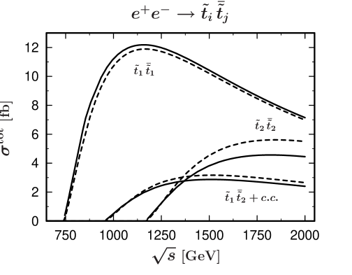
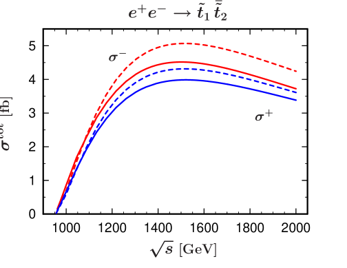
Figure 5: Left: The total cross-sections for stop pair production (all channels) at tree-level {dashed} and with complete corrections {solid}. Right: The total cross-sections for polarized beams: $\sigma^{-}$ stands for $P_{-}=-0.8,\,P_{+}=0.6$ and $\sigma^{+}$ for $P_{-}=0.8,\,P_{+}=-0.6$.

  

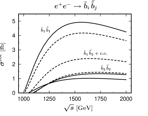
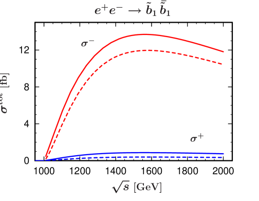
Figure 6: Left: The total cross-sections for sbottom pair production (all channels) at tree-level {dashed} and with complete corrections {solid}. Right: The total cross-sections for polarized beams $\sigma^{-}$ stands for $P_{-}=-0.8,\,P_{+}=0.6$ and $\sigma^{+}$ for $P_{-}=0.8,\,P_{+}=-0.6$.

For each sfermion type we show an unpolarized case (left) and a case where the beams are polarized (right). We take two sets of polarizations, either $P_{-}=-0.8$ and $P_{+}=0.6$ or $P_{-}=0.8$ and $P_{+}=-0.6$. The difference to the earlier calculations letter ; hollik are the QED corrections which give a negative contribution near the threshold due to the known soft-photon behaviour. The QED corrections are substantial (as can be checked when comparing the results of this paper with those of letter ) and cannot to be neglected. The plots on the right-hand side of Fig. 5-8 show the effect of beams polarization on the radiative corrections. Polarization and its effects are best seen in other observables which we discuss in the following.

  

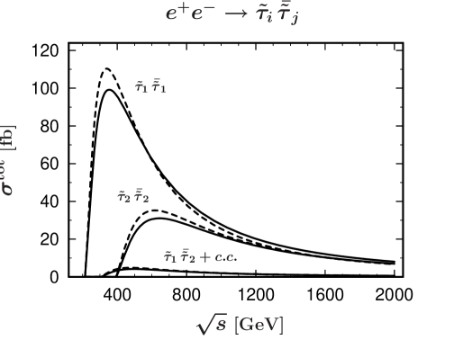
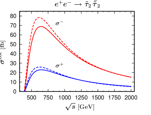
Figure 7: Left: The total cross-sections for stau pair production (all channels) at tree-level {dashed} and with complete corrections {solid}. Right: The total cross-sections for polarized beams $\sigma^{-}$ stands for $P_{-}=-0.8,\,P_{+}=0.6$ and $\sigma^{+}$ for $P_{-}=0.8,\,P_{+}=-0.6$.

  

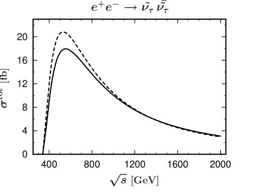
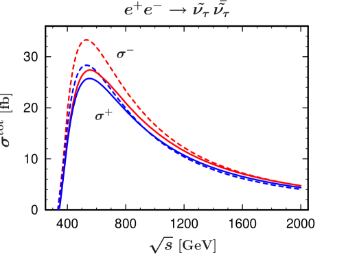
Figure 8: Left: The total cross-sections for tau-sneutrino pair production at tree-level {dashed} and with complete corrections {solid}. Right: The total cross-sections for polarized beams $\sigma^{-}$ stands for $P_{-}=-0.8,\,P_{+}=0.6$ and $\sigma^{+}$ for $P_{-}=0.8,\,P_{+}=-0.6$.

  

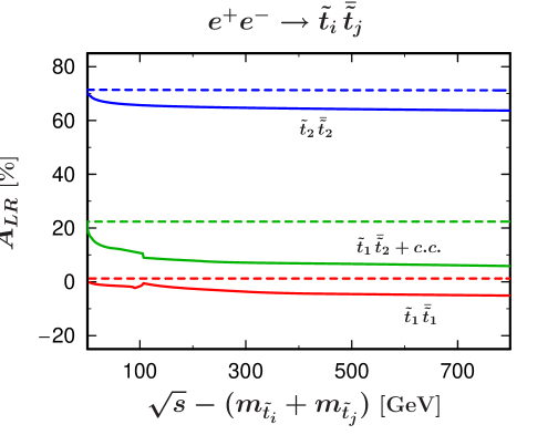
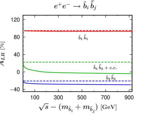
Figure 9: Left: The left-right asymmetry for stop pair production at tree-level {dashed} and with complete corrections {solid}. Right: The left-right asymmetry for sbottom pair production at tree-level {dashed} and with complete corrections {solid}.

The Figs. 9-12 show the left-right and forward-backward asymmetries for different final states as defined in Eq. (20). Owing to the fact that at tree level there is only a s-channel contribution the $\sqrt{s}$-dependence drops out in the left-right asymmetry, making it to a good approximation constant. The $\sqrt{s}$-dependence is then a result of the one-loop corrections. Notice that the corrections are substantial especially in the ${\tilde{t}}_{1}{\tilde{t}}_{2}$, ${\tilde{b}}_{1}{\tilde{b}}_{2}$, ${\tilde{\tau}}_{1}{\tilde{\tau}}_{2}$, as well as in the $\tilde{\nu}_{\tau}\tilde{\nu}_{\tau}$ channel, where there is only a $Z$ exchange at tree-level.
As we have already mentioned, there is no tree-level contribution to the forward-backward asymmetry and thus the asymmetry is loop-induced. In the calculation of the forward-backward asymmetry at one-loop one has to define the forward direction, in particular for the contributions coming from the photon radiation . We define it by $\sigma_{F}\equiv\sigma(\cos\theta_{\vec{p_{1}}\vec{k_{1,2}}}\geq 0)$ where $\theta_{\vec{p_{1}}\vec{k_{1,2}}}$ is the angle between the incoming electron and the outgoing sfermion with negative isospin. As an additional feature, we also show the forward-backward asymmetry for polarized beams where the polarizations are $P_{-}=-0.8$ and $P_{+}=0.6$. In general, one sees that the asymmetries receive sizeable corrections and thus justify the higher-order calculation.

  

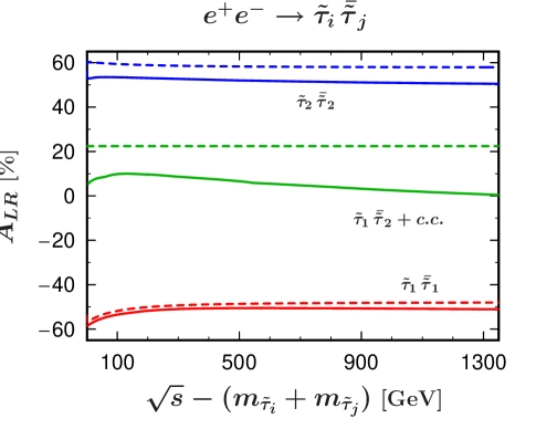
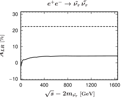
Figure 10: Left: The left-right asymmetry for stau pair production at tree-level {dashed} and with complete corrections {solid}. Right: The left-right asymmetry for tau-sneutrino pair production at tree-level {dashed} and with complete corrections {solid}.

  

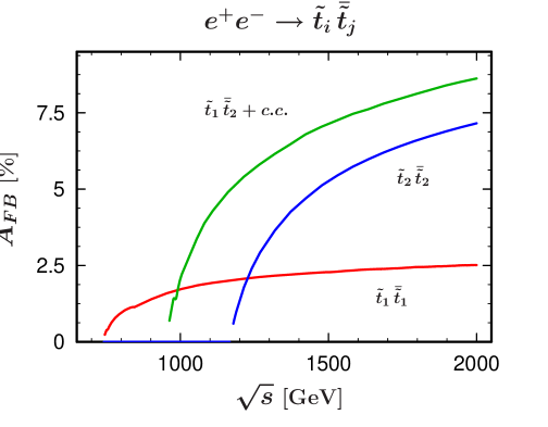
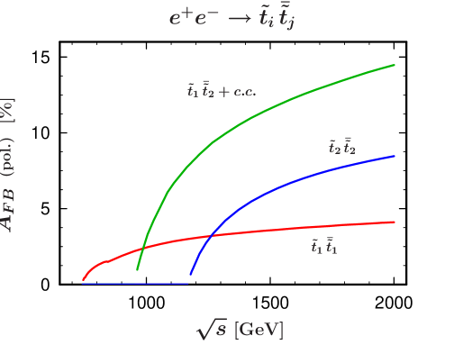
Figure 11: Left: The forward-backward asymmetry for stop pair production (no tree-level contribution) for unpolarized beams. Right: The forward-backward asymmetry for stop pair production with polarized beams $P_{-}=-0.8,\,P_{+}=0.6$.

  

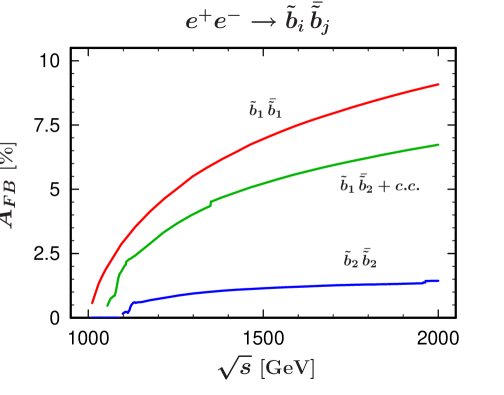
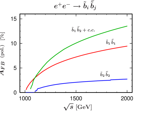
Figure 12: Left: The forward-backward asymmetry for sbottom pair production (no tree-level contribution) for unpolarized beams. Right: The forward-backward asymmetry for sbottom pair production with polarized beams $P_{-}=-0.8,\,P_{+}=0.6$.

VI Conclusion

We have calculated the full $\cal{O}(\alpha)$ corrections to stop, sbottom, stau and tau-sneutrino production in the MSSM. We have presented the details of our analytical calculation which was also checked by the computer algebra tools FeynArts and FormCalc feyn . The results extend our previous calculations SUSY-QCD-H ; Yukawa ; letter by including also QED contributions and the real photon radiation. We have also used the structure function approach slicing2 to include some higher order effects. Moreover, the whole calculation was extended to the case of polarized $e^{\pm}$-beams.
In the numerical analysis, we have studied only one specific scenario based on the SPS1a’ benchmark point defined in the SPA project. We have transformed the input parameters into the on-shell renormalization scheme which we have used throughout the paper. The numerical results show the total cross-sections and asymmetries with the effect of the $\cal{O}(\alpha)$ corrections. These are found to be sizeable (in some cases up to 15% and larger), and in particular the forward-backward asymmetry is only due to higher order corrections.

Acknowledgements
We thank W. Öller for useful discussions. The authors acknowledge support from EU under the HPRN-CT-2000-00149 network programme and the “Fonds zur Förderung der wissenschaftlichen Forschung” of Austria, project No. P16592-N02.

Appendix A Vertex corrections

Here we give the explicit form of the electroweak contributions to the vertex corrections which are depicted in Fig. 2. For SUSY-QCD contributions we refer to SUSY-QCD-H . All couplings used in this paper can be found in chrislet .

The vertex corrections $(\delta e_{f})_{ij}^{(v)}$ and $(\delta a_{f})_{ij}^{(v)}$ (or $\delta e_{L,R}^{(v)}$ and $\delta a_{L,R}^{(v)}$) originate from the diagrams in Fig. 2 with $\gamma$, $Z$-boson exchange, respectively.
The vertex corrections to the right vertex $(\delta e_{f})_{ij}^{(v)}$ and $(\delta a_{f})_{ij}^{(v)}$ are defined on the amplitude level from the corresponding diagrams. The general form of the amplitude is given by

$${\cal{M}}=\frac{i}{(4\pi)^{2}}\frac{X_{V}}{s-m_{V}^{2}}\bar{v}(p_{2})\,\gamma^{\mu}(Y^{V}_{L}\,P_{L}+Y^{V}_{R}\,P_{R})\,u(p_{1})\left[A_{ij}\,(k_{1}-k_{2})_{\mu}+B_{ij}\,(k_{1}+k_{2})_{\mu}\right]\,.$$ (89)

For $X_{V}$ and $Y^{V}_{L,R}$ with $V=\gamma,Z$ we have

$$X_{\gamma}=e\,,\qquad Y^{\gamma}_{L,R}=K_{L,R}\,,\qquad X_{Z}=-g_{Z}\,,\qquad Y^{Z}_{L,R}=C_{L,R}\,.$$ (90)

We use the form-factor $A_{ij}$ (the other form-factor vanishes in $|{\cal{M}}|^{2}$) to define the vertex correction $(\delta e_{f})_{ij}^{(v)}$ and $(\delta a_{f})_{ij}^{(v)}$ as

$$(\delta e_{f})_{ij}^{(v)}=-\frac{1}{(4\pi)^{2}}\frac{1}{e}\,A_{ij}\,,\qquad\quad(\delta a_{f})_{ij}^{(v)}=-\frac{1}{(4\pi)^{2}}\frac{4\,c_{W}}{g}\,A_{ij}\,.$$ (91)

The explicit formulas for $(\delta e_{f})_{ij}^{(v)}$ and $(\delta a_{f})_{ij}^{(v)}$ are given below in the Appendices A.1 and A.2.
The vertex corrections to the left vertex, $\delta e_{L,R}^{(v)}$ and $\delta a_{L,R}^{(v)}$, include corrections to the two chiral parts of the electron photon/$Z$-boson vertex. The generic form is

$${\cal{M}}=\frac{i}{(4\pi)^{2}}\frac{(X_{V})_{ij}}{s-m_{V}^{2}}\,\bar{v}(p_{2})\left[\,A_{L}\gamma^{\mu}\,P_{L}+A_{R}\gamma^{\mu}\,P_{R}+B_{L}P_{L}(p_{1}-p_{2})^{\mu}+B_{R}P_{R}(p_{1}-p_{2})^{\mu}\right.$$

$$\left.+C_{L}P_{L}(p_{1}+p_{2})^{\mu}+C_{R}P_{R}(p_{1}+p_{2})^{\mu}\,\right]u(p_{1})(k_{1}-k_{2})_{\mu}\,,$$ (92)

where $(X_{V})_{ij}$ ($V=\gamma,Z$) stands for

$$(X_{\gamma})_{ij}=-e\,e_{f}\delta_{ij}\,,\qquad\qquad(X_{Z})_{ij}=-\frac{g_{Z}}{4}a^{f}_{ij}\,.$$ (93)

From this generic structure only the form-factors $A_{L,R}$ survive. We define the vertex corrections as

$$\delta e_{L,R}^{(v)}=\frac{1}{(4\pi)^{2}}\frac{1}{e}\,A_{L,R}\,,\qquad\quad\delta a_{L,R}^{(v)}=-\frac{1}{(4\pi)^{2}}\frac{c_{W}}{g}\,A_{L,R}\,.$$ (94)

The contributions to the vertex corrections $\delta e_{L,R}^{(v)}$ and $\delta a_{L,R}^{(v)}$ are given in the Appendices A.3 and A.4.

A.1 Corrections to $\gamma{\tilde{f}}_{i}{\tilde{f}}_{j}$ vertex

The vertex correction $(\delta e_{f})_{ij}^{(v)}$ is composed of contributions from different classes of diagrams as follows,

$$(\delta e_{f})_{ij}^{(v)}=(\delta e_{f})_{ij}^{(v,\tilde{\chi})}+(\delta e_{f})_{ij}^{(v,SSS)}+(\delta e_{f})_{ij}^{(v,V\!{\tilde{f}}\!{\tilde{f}})}+(\delta e_{f})_{ij}^{(v,S\!S\!V+S\!V\!S)}+(\delta e_{f})_{ij}^{(v,S\!V\!V)}+(\delta e_{f})_{ij}^{(v,S\!V)}\,.$$ (95)

In the following we use the standard two- and three-point functions $B_{i}$ and $C_{i}$ from PaVe in the conventions of Denner . We introduce the following standard set of arguments $C_{i}\equiv C_{i}\big{(}m_{{\tilde{f}}_{i}}^{2},s,m_{{\tilde{f}}_{j}}^{2},M_{0}^{2},M_{1}^{2},M_{2}^{2}\big{)}$ to be used in the generic functions ${\cal S}$.

The first contribution coming from the exchange of one or two gauginos is

$$(\delta e_{f})_{ij}^{(v,\tilde{\chi})} = \frac{1}{(4\pi)^{2}}\sum_{k,l=1}^{2}{\cal S}^{F\!F\!F}_{ij}\Big{(}m_{f^{\prime}},m_{\tilde{\chi}^{+}_{k}},m_{\tilde{\chi}^{+}_{l}};2I_{f}^{3L}\delta_{kl},2I_{f}^{3L}\delta_{kl},k^{\tilde{f}}_{ik},l^{\tilde{f}}_{ik},l^{\tilde{f}}_{jl},k^{\tilde{f}}_{jl}\Big{)}$$ (96)

$$+\frac{1}{(4\pi)^{2}}\sum_{k=1}^{4}{\cal S}^{F\!F\!F}_{ij}\Big{(}m_{\tilde{\chi}^{0}_{k}},m_{f},m_{f};e_{f},e_{f},b^{\tilde{f}}_{ik},a^{\tilde{f}}_{ik},a^{\tilde{f}}_{jk},b^{\tilde{f}}_{jk}\Big{)}$$

$$+\frac{1}{(4\pi)^{2}}\sum_{k=1}^{2}{\cal S}^{F\!F\!F}_{ij}\Big{(}m_{\tilde{\chi}^{+}_{k}},m_{f^{\prime}},m_{f^{\prime}};e_{f^{\prime}},e_{f^{\prime}},k^{\tilde{f}}_{ik},l^{\tilde{f}}_{ik},l^{\tilde{f}}_{jk},k^{\tilde{f}}_{jk}\Big{)}\,,$$

with the generic vertex function

$${\cal S}^{F\!F\!F}_{ij}\big{(}M_{0},M_{1},M_{2};g_{0}^{R},g_{0}^{L},g_{1}^{R},g_{1}^{L},g_{2}^{R},g_{2}^{L}\big{)}~{}=~{}M_{0}M_{2}\big{(}g_{0}^{L}g_{1}^{L}g_{2}^{L}+g_{0}^{R}g_{1}^{R}g_{2}^{R}\big{)}\big{(}C_{0}+C_{1}+C_{2}\big{)}$$ (97)

$$+M_{0}M_{1}\big{(}g_{0}^{L}g_{1}^{R}g_{2}^{R}+g_{0}^{R}g_{1}^{L}g_{2}^{L}\big{)}\big{(}C_{0}+C_{1}+C_{2}\big{)}+M_{1}M_{2}\big{(}g_{0}^{L}g_{1}^{R}g_{2}^{L}+g_{0}^{R}g_{1}^{L}g_{2}^{R}\big{)}\big{(}C_{1}+C_{2}\big{)}$$

$$+\big{(}g_{0}^{L}g_{1}^{L}g_{2}^{R}+g_{0}^{R}g_{1}^{R}g_{2}^{L}\big{)}\Big{(}B_{0}\big{(}s,M_{1}^{2},M_{2}^{2}\big{)}+M_{0}^{2}\big{(}2C_{0}+C_{1}+C_{2}\big{)}+m_{{\tilde{f}}_{i}}^{2}C_{1}+m_{{\tilde{f}}_{j}}^{2}C_{2}\Big{)}\,.$$

The corrections due to graphs with 3 scalar particles in the loop are given by

$$(\delta e_{f})_{ij}^{(v,SSS)} = -\frac{1}{(4\pi)^{2}}\,2I_{f}^{3L}\sum_{k,m=1}^{2}\!G^{{\tilde{f}}{\tilde{f}}^{\prime}}_{imk}G^{{\tilde{f}}{\tilde{f}}^{\prime}}_{jmk}\big{(}C_{0}+C_{1}+C_{2}\big{)}\big{(}m_{{\tilde{f}}_{i}}^{2},s,m_{{\tilde{f}}_{j}}^{2},m_{{\tilde{f}}^{\prime}_{m}}^{2},m_{H_{k}^{+}}^{2},m_{H_{k}^{+}}^{2}\big{)}$$ (98)

$$-\frac{1}{(4\pi)^{2}}\,e_{f}\sum_{k,m=1}^{2}\!G^{{\tilde{f}}}_{imk}G^{{\tilde{f}}}_{mjk}\big{(}C_{0}+C_{1}+C_{2}\big{)}\big{(}m_{{\tilde{f}}_{i}}^{2},s,m_{{\tilde{f}}_{j}}^{2},m_{H_{k}^{0}}^{2},m_{{\tilde{f}}_{m}}^{2},m_{{\tilde{f}}_{m}}^{2}\big{)}$$

$$-\frac{1}{(4\pi)^{2}}\,e_{f^{\prime}}\sum_{k,m=1}^{2}\!G^{{\tilde{f}}{\tilde{f}}^{\prime}}_{imk}G^{{\tilde{f}}{\tilde{f}}^{\prime}}_{jmk}\big{(}C_{0}+C_{1}+C_{2}\big{)}\big{(}m_{{\tilde{f}}_{i}}^{2},s,m_{{\tilde{f}}_{j}}^{2},m_{H_{k}^{+}}^{2},m_{{\tilde{f}}^{\prime}_{m}}^{2},m_{{\tilde{f}}^{\prime}_{m}}^{2}\big{)}\,.$$

The graphs with one vector particle ($\gamma,Z^{0},W^{+}$) and two sfermions in the loop yield

$$(\delta e_{f})_{ij}^{(v,V\!{\tilde{f}}\!{\tilde{f}})} = \frac{1}{(4\pi)^{2}}\,e^{2}e_{f}^{3}\,\delta_{ij}\,{\cal S}^{V\!{\tilde{f}}\!{\tilde{f}}}_{ij}\big{(}\lambda,m_{{\tilde{f}}_{i}},m_{{\tilde{f}}_{i}}\big{)}+\frac{1}{(4\pi)^{2}}\,g_{Z}^{2}\,e_{f}\sum_{m=1}^{2}z^{\tilde{f}}_{im}\,z^{\tilde{f}}_{mj}\,{\cal S}^{V\!{\tilde{f}}\!{\tilde{f}}}_{ij}\big{(}m_{Z},m_{{\tilde{f}}_{m}},m_{{\tilde{f}}_{m}}\big{)}$$ (99)

$$+\frac{1}{(4\pi)^{2}}\,\frac{g^{2}}{2}\,e_{f^{\prime}}R^{\tilde{f}}_{i1}R^{\tilde{f}}_{j1}\sum_{m=1}^{2}\big{(}R^{{\tilde{f}}^{\prime}}_{m1}\big{)}^{2}\,{\cal S}^{V\!{\tilde{f}}\!{\tilde{f}}}_{ij}\big{(}m_{W},m_{{\tilde{f}}^{\prime}_{m}},m_{{\tilde{f}}^{\prime}_{m}}\big{)}\,,$$

where ${\cal S}^{V\!{\tilde{f}}\!{\tilde{f}}}_{ij}(\ldots)$ is a short form for

$${\cal S}^{V\!{\tilde{f}}\!{\tilde{f}}}_{ij}\big{(}M_{0},M_{1},M_{2}\big{)}~{}=~{}4C_{00}+\big{(}M_{0}^{2}-2s+2m_{{\tilde{f}}_{i}}^{2}+2m_{{\tilde{f}}_{j}}^{2}\big{)}\big{(}C_{0}+C_{1}+C_{2}\big{)}$$

$$+\big{(}2m_{{\tilde{f}}_{i}}^{2}+2m_{{\tilde{f}}_{j}}^{2}-s\big{)}\big{(}C_{1}+C_{2}+C_{11}+2C_{12}+C_{22}\big{)}+\big{(}m_{{\tilde{f}}_{i}}^{2}-m_{{\tilde{f}}_{j}}^{2}\big{)}\big{(}C_{1}-C_{2}+C_{11}-C_{22}\big{)}\,.$$

From the diagrams with one $W^{+}$-boson, one Goldstone boson $G^{+}$ and a sfermion we obtain

$$(\delta e_{f})_{ij}^{(v,S\!S\!V+S\!V\!S)} = \frac{1}{(4\pi)^{2}}\,\frac{g\,m_{W}}{2\sqrt{2}}\sum_{m=1}^{2}\left(R^{\tilde{f}}_{i1}G^{{\tilde{f}}{\tilde{f}}^{\prime}}_{jm2}+R^{\tilde{f}}_{j1}G^{{\tilde{f}}{\tilde{f}}^{\prime}}_{im2}\right)R^{{\tilde{f}}^{\prime}}_{m1}$$ (101)

$$\hskip 75.0pt\times~{}\big{(}C_{0}-C_{1}-C_{2}\big{)}\big{(}m_{{\tilde{f}}_{i}}^{2},s,m_{{\tilde{f}}_{j}}^{2},m_{{\tilde{f}}^{\prime}_{m}}^{2},m_{W}^{2},m_{W}^{2}\big{)}\,,$$

and with the generic scalar–vector–vector vertex function

$${\cal S}^{S\!V\!V}_{ij}\big{(}M_{0},M_{1},M_{2}\big{)}~{}=~{}2B_{0}\big{(}s,M_{1}^{2},M_{2}^{2}\big{)}-2C_{00}+\Big{(}\frac{s}{2}+2M_{0}^{2}\Big{)}C_{0}-s\big{(}C_{1}+C_{2}\big{)}$$ (102)

$$-\frac{1}{2}\big{(}m_{{\tilde{f}}_{i}}^{2}-m_{{\tilde{f}}_{j}}^{2}\big{)}\big{(}C_{1}-C_{2}+C_{11}-C_{22}\big{)}-\frac{1}{2}\big{(}2m_{{\tilde{f}}_{i}}^{2}+2m_{{\tilde{f}}_{j}}^{2}-s\big{)}\big{(}C_{11}+2C_{12}+C_{22}\big{)}$$

the correction due to the exchange of two $W^{+}$-bosons and one sfermion reads

$$(\delta e_{f})_{ij}^{(v,S\!V\!V)} = \frac{1}{(4\pi)^{2}}\,g^{2}\,I_{f}^{3L}R^{\tilde{f}}_{i1}R^{\tilde{f}}_{j1}\sum_{m=1}^{2}\big{(}R^{{\tilde{f}}^{\prime}}_{m1}\big{)}^{2}\,{\cal S}^{S\!V\!V}_{ij}\big{(}m_{{\tilde{f}}^{\prime}_{m}},m_{W},m_{W}\big{)}\,.$$ (103)

The contributions from one sfermion and one vector particle ($\gamma,Z^{0},W^{+}$) can be expressed as

$$(\delta e_{f})_{ij}^{(v,S\!V)} = -\frac{1}{(4\pi)^{2}}\,2e^{2}e_{f}^{3}\,\delta_{ij}\big{(}2B_{0}+B_{1}\big{)}\big{(}m_{{\tilde{f}}_{i}}^{2},\lambda^{2},m_{{\tilde{f}}_{i}}^{2}\big{)}$$ (104)

$$-\frac{1}{(4\pi)^{2}}\,g_{Z}^{2}\,e_{f}\sum_{m=1}^{2}z^{\tilde{f}}_{im}z^{\tilde{f}}_{jm}\big{(}2B_{0}+B_{1}\big{)}\big{(}m_{{\tilde{f}}_{i}}^{2},m_{Z}^{2},m_{{\tilde{f}}_{m}}^{2}\big{)}\qquad+(i\leftrightarrow j)$$

$$-\frac{1}{(4\pi)^{2}}\,\frac{g^{2}}{4}\,Y^{f}_{L}R^{\tilde{f}}_{i1}R^{\tilde{f}}_{j1}\sum_{m=1}^{2}\big{(}R^{{\tilde{f}}^{\prime}}_{m1}\big{)}^{2}\big{(}2B_{0}+B_{1}\big{)}\big{(}m_{{\tilde{f}}_{i}}^{2},m_{W}^{2},m_{{\tilde{f}}^{\prime}_{m}}^{2}\big{)}\qquad+(i\leftrightarrow j)$$

with $Y_{L}^{f}=2(I_{f}^{3L}-e_{f})$. The symbol $(i\leftrightarrow j)$ denotes the previous term with the indices $i$ and $j$ interchanged.

A.2 Corrections to $Z^{0}{\tilde{f}}_{i}{\tilde{f}}_{j}$ vertex

The corrections to the $Z^{0}{\tilde{f}}_{i}{\tilde{f}}_{j}$ vertex have the same components as in Eq. (95). Using the same abbreviations for the generic vertex functions as in the previous section we get for the single contributions:

$$(\delta a_{f})_{ij}^{(v,\tilde{\chi})} = -\frac{4}{(4\pi)^{2}}\sum_{k,l=1}^{4}{\cal S}^{F\!F\!F}_{ij}\Big{(}m_{f},m_{\tilde{\chi}^{0}_{k}},m_{\tilde{\chi}^{0}_{l}};O_{kl}^{{}^{\prime\prime}R},O_{kl}^{{}^{\prime\prime}L},b^{\tilde{f}}_{ik},a^{\tilde{f}}_{ik},a^{\tilde{f}}_{jl},b^{\tilde{f}}_{jl}\Big{)}$$ (105)

$$-\frac{4}{(4\pi)^{2}}\,2I^{3L}_{f}\sum_{k,l=1}^{2}{\cal S}^{F\!F\!F}_{ij}\Big{(}m_{f^{\prime}},m_{\tilde{\chi}^{+}_{k}},m_{\tilde{\chi}^{+}_{l}};\widetilde{O}_{kl}^{{}^{\prime}R},\widetilde{O}_{kl}^{{}^{\prime}L},k^{\tilde{f}}_{ik},l^{\tilde{f}}_{ik},l^{\tilde{f}}_{jl},k^{\tilde{f}}_{jl}\Big{)}$$

$$+\frac{4}{(4\pi)^{2}}\sum_{k=1}^{4}{\cal S}^{F\!F\!F}_{ij}\Big{(}m_{\tilde{\chi}^{0}_{k}},m_{f},m_{f};C^{f}_{R},C^{f}_{L},b^{\tilde{f}}_{ik},a^{\tilde{f}}_{ik},a^{\tilde{f}}_{jk},b^{\tilde{f}}_{jk}\Big{)}$$

$$+\frac{4}{(4\pi)^{2}}\sum_{k=1}^{2}{\cal S}^{F\!F\!F}_{ij}\Big{(}m_{\tilde{\chi}^{+}_{k}},m_{f^{\prime}},m_{f^{\prime}};C^{f^{\prime}}_{R},C^{f^{\prime}}_{L},k^{\tilde{f}}_{ik},l^{\tilde{f}}_{ik},l^{\tilde{f}}_{jk},k^{\tilde{f}}_{jk}\Big{)}\,,$$

with $\widetilde{O}_{kl}^{{}^{\prime}L/R}=O_{kl}^{{}^{\prime}L/R}$ for up-type sfermions (up-squarks and sneutrinos) and $\widetilde{O}_{kl}^{{}^{\prime}L/R}=O_{kl}^{{}^{\prime}R/L}$ for down-type sfermions (down-squarks and sleptons),

$$(\delta a_{f})_{ij}^{(v,SSS)} = \frac{2i}{(4\pi)^{2}}\sum_{k,m=1}^{2}\sum_{l=3}^{4}\!R_{k,l-2}(\beta-\alpha)\,G^{{\tilde{f}}}_{imk}G^{{\tilde{f}}}_{mjl}\big{(}C_{0}+C_{1}+C_{2}\big{)}\big{(}m_{{\tilde{f}}_{i}}^{2},s,m_{{\tilde{f}}_{j}}^{2},m_{{\tilde{f}}_{m}}^{2},m_{H_{k}^{0}}^{2},m_{H_{l}^{0}}^{2}\big{)}$$ (106)

$$-\frac{2i}{(4\pi)^{2}}\sum_{k=3}^{4}\sum_{l,m=1}^{2}\!R_{l,k-2}(\beta-\alpha)\,G^{{\tilde{f}}}_{imk}G^{{\tilde{f}}}_{mjl}\big{(}C_{0}+C_{1}+C_{2}\big{)}\big{(}m_{{\tilde{f}}_{i}}^{2},s,m_{{\tilde{f}}_{j}}^{2},m_{{\tilde{f}}_{m}}^{2},m_{H_{k}^{0}}^{2},m_{H_{l}^{0}}^{2}\big{)}$$

$$-\frac{4}{(4\pi)^{2}}\,I_{f}^{3L}\cos 2\theta_{W}\sum_{k,m=1}^{2}\!G^{{\tilde{f}}{\tilde{f}}^{\prime}}_{imk}G^{{\tilde{f}}{\tilde{f}}^{\prime}}_{jmk}\big{(}C_{0}+C_{1}+C_{2}\big{)}\big{(}m_{{\tilde{f}}_{i}}^{2},s,m_{{\tilde{f}}_{j}}^{2},m_{{\tilde{f}}^{\prime}_{m}}^{2},m_{H_{k}^{+}}^{2},m_{H_{k}^{+}}^{2}\big{)}$$

$$-\frac{4}{(4\pi)^{2}}\sum_{k,m,n=1}^{2}\!z^{\tilde{f}}_{mn}G^{{\tilde{f}}}_{imk}G^{{\tilde{f}}}_{njk}\big{(}C_{0}+C_{1}+C_{2}\big{)}\big{(}m_{{\tilde{f}}_{i}}^{2},s,m_{{\tilde{f}}_{j}}^{2},m_{H_{k}^{0}}^{2},m_{{\tilde{f}}_{m}}^{2},m_{{\tilde{f}}_{n}}^{2}\big{)}$$

$$-\frac{4}{(4\pi)^{2}}\sum_{k,m,n=1}^{2}\!z^{{\tilde{f}}^{\prime}}_{mn}G^{{\tilde{f}}{\tilde{f}}^{\prime}}_{imk}G^{{\tilde{f}}{\tilde{f}}^{\prime}}_{jnk}\big{(}C_{0}+C_{1}+C_{2}\big{)}\big{(}m_{{\tilde{f}}_{i}}^{2},s,m_{{\tilde{f}}_{j}}^{2},m_{H_{k}^{+}}^{2},m_{{\tilde{f}}^{\prime}_{m}}^{2},m_{{\tilde{f}}^{\prime}_{n}}^{2}\big{)}\,,$$

$$(\delta a_{f})_{ij}^{(v,V\!{\tilde{f}}\!{\tilde{f}})} = \frac{4}{(4\pi)^{2}}\,e^{2}e_{f}^{2}\,z^{\tilde{f}}_{ij}\,{\cal S}^{V\!{\tilde{f}}\!{\tilde{f}}}_{ij}\big{(}\lambda,m_{{\tilde{f}}_{i}},m_{{\tilde{f}}_{j}}\big{)}+\frac{4}{(4\pi)^{2}}\,g_{Z}^{2}\sum_{m,n=1}^{2}\!z^{\tilde{f}}_{im}\,z^{\tilde{f}}_{mn}\,z^{\tilde{f}}_{nj}\,{\cal S}^{V\!{\tilde{f}}\!{\tilde{f}}}_{ij}\big{(}m_{Z},m_{{\tilde{f}}_{m}},m_{{\tilde{f}}_{n}}\big{)}$$ (107)

$$+\frac{4}{(4\pi)^{2}}\,\frac{g^{2}}{2}\,R^{\tilde{f}}_{i1}R^{\tilde{f}}_{j1}\sum_{m,n=1}^{2}\!R^{{\tilde{f}}^{\prime}}_{m1}R^{{\tilde{f}}^{\prime}}_{n1}\,{\cal S}^{V\!{\tilde{f}}\!{\tilde{f}}}_{ij}\big{(}m_{W},m_{{\tilde{f}}^{\prime}_{m}},m_{{\tilde{f}}^{\prime}_{n}}\big{)}\,,$$

$$(\delta a_{f})_{ij}^{(v,S\!S\!V+S\!V\!S)} =$$ (108)

$$-\frac{1}{(4\pi)^{2}}\sqrt{2}\,g\,s_{W}^{2}m_{W}\!\sum_{m=1}^{2}\!\left(R^{\tilde{f}}_{i1}G^{{\tilde{f}}{\tilde{f}}^{\prime}}_{jm2}+R^{\tilde{f}}_{j1}G^{{\tilde{f}}{\tilde{f}}^{\prime}}_{im2}\right)R^{{\tilde{f}}^{\prime}}_{m1}\big{(}C_{0}-C_{1}-C_{2}\big{)}\big{(}m_{{\tilde{f}}_{i}}^{2},s,m_{{\tilde{f}}_{j}}^{2},m_{{\tilde{f}}^{\prime}_{m}}^{2},m_{W}^{2},m_{W}^{2}\big{)}$$

$$+\frac{1}{(4\pi)^{2}}\,2\,g_{Z}\,m_{Z}\!\sum_{k,m=1}^{2}\!R_{k_{2}}(\beta-\alpha)\,z^{\tilde{f}}_{im}G^{{\tilde{f}}}_{mjk}\big{(}C_{0}-C_{1}-C_{2}\big{)}\big{(}m_{{\tilde{f}}_{i}}^{2},s,m_{{\tilde{f}}_{j}}^{2},m_{{\tilde{f}}_{m}}^{2},m_{Z}^{2},m_{H_{k}^{0}}^{2}\big{)}$$

$$+\frac{1}{(4\pi)^{2}}\,2\,g_{Z}\,m_{Z}\!\sum_{k,m=1}^{2}\!R_{k_{2}}(\beta-\alpha)\,z^{\tilde{f}}_{mj}G^{{\tilde{f}}}_{imk}\big{(}C_{0}-C_{1}-C_{2}\big{)}\big{(}m_{{\tilde{f}}_{i}}^{2},s,m_{{\tilde{f}}_{j}}^{2},m_{{\tilde{f}}_{m}}^{2},m_{H_{k}^{0}}^{2},m_{Z}^{2}\big{)}\,,$$

$$(\delta a_{f})_{ij}^{(v,S\!V\!V)} = \frac{4}{(4\pi)^{2}}\,g^{2}\,c_{W}^{2}\,I_{f}^{3L}R^{\tilde{f}}_{i1}R^{\tilde{f}}_{j1}\sum_{m=1}^{2}\big{(}R^{{\tilde{f}}^{\prime}}_{m1}\big{)}^{2}\,{\cal S}^{S\!V\!V}_{ij}\big{(}m_{{\tilde{f}}^{\prime}_{m}},m_{W},m_{W}\big{)}\,,$$ (109)

$$(\delta a_{f})_{ij}^{(v,S\!V)} = -\frac{4}{(4\pi)^{2}}\,e^{2}e_{f}^{2}\,z^{\tilde{f}}_{ij}\big{(}2B_{0}+B_{1}\big{)}\big{(}m_{{\tilde{f}}_{i}}^{2},\lambda^{2},m_{{\tilde{f}}_{i}}^{2}\big{)}\qquad+(i\leftrightarrow j)$$ (110)

$$-\frac{4}{(4\pi)^{2}}\,g_{Z}^{2}\,\sum_{m=1}^{2}z^{\tilde{f}}_{im}\tilde{z}^{\tilde{f}}_{jm}\big{(}2B_{0}+B_{1}\big{)}\big{(}m_{{\tilde{f}}_{i}}^{2},m_{Z}^{2},m_{{\tilde{f}}_{m}}^{2}\big{)}\qquad+(i\leftrightarrow j)$$

$$+\frac{1}{(4\pi)^{2}}\,e^{2}\,Y^{f}_{L}\,R^{\tilde{f}}_{i1}R^{\tilde{f}}_{j1}\sum_{m=1}^{2}\big{(}R^{{\tilde{f}}^{\prime}}_{m1}\big{)}^{2}\big{(}2B_{0}+B_{1}\big{)}\big{(}m_{{\tilde{f}}_{i}}^{2},m_{W}^{2},m_{{\tilde{f}}^{\prime}_{m}}^{2}\big{)}\qquad+(i\leftrightarrow j)\,.$$

A.3 Corrections to $\gamma e^{+}e^{-}$ vertex

In the following we list the analytic formulas of the vertex corrections to the electron–positron–photon vertex. We only give the right-handed coefficients of the generic vertex functions, ${\cal F}_{\!R}^{(\cdots)}$ as the coefficients ${\cal F}_{\!L}^{(\cdots)}$ can be obtained by exchanging the indices $R$ and $L$, i. e. ${\cal F}_{\!L}^{(\cdots)}={\cal F}_{\!R}^{(\cdots)}(R\leftrightarrow L)$.
In the remaining vertex corrections we use the standard set of arguments for the whole class of $C$-functions $C\equiv C\big{(}m_{e}^{2},s,m_{e}^{2},M_{0}^{2},M_{1}^{2},M_{2}^{2}\big{)}$.
The vertex correction $\delta e_{L,R}^{(v)}$ is split into the following classes:

$$\delta e_{L,R}^{(v)}=\delta e_{L,R}^{(v,{\tilde{f}}\tilde{\chi}\tilde{\chi})}+\delta e_{R}^{(v,\tilde{\chi}{\tilde{f}}{\tilde{f}})}+\delta e_{L,R}^{(v,V\!F\!F)}+\delta e_{L,R}^{(v,F\!V\!V)}$$ (111)

The contribution from one sfermion and two gauginos in the loop is given by

$$\delta e_{L,R}^{(v,{\tilde{f}}\tilde{\chi}\tilde{\chi})} = \frac{1}{(4\pi)^{2}}\sum_{k=1}^{2}{\cal F}_{\!L,R}^{S\!F\!F}\Big{(}m_{\tilde{\nu}_{e}},m_{\tilde{\chi}^{+}_{k}},m_{\tilde{\chi}^{+}_{k}};1,1,l^{\tilde{\nu}_{e}}_{1k},k^{\tilde{\nu}_{e}}_{1k},k^{\tilde{\nu}_{e}}_{1k},l^{\tilde{\nu}_{e}}_{1k}\Big{)}\,,$$ (112)

where we have used the generic vertex function

$${\cal F}_{\!R}^{S\!F\!F}\big{(}M_{0},M_{1},M_{2};g_{0}^{R},g_{0}^{L},g_{1}^{R},g_{1}^{L},g_{2}^{R},g_{2}^{L}\big{)}~{}=~{}-g_{0}^{L}g_{1}^{L}g_{2}^{R}\Big{(}2C_{00}-B_{0}\big{(}s,M_{1}^{2},M_{2}^{2}\big{)}\Big{)}$$

$$-\big{(}g_{0}^{R}h_{1}^{RL}h_{2}^{LR}-g_{0}^{L}g_{1}^{L}g_{2}^{R}M_{0}^{2}\big{)}C_{0}-\big{(}g_{0}^{R}g_{1}^{R}h_{2}^{LR}-g_{0}^{L}g_{2}^{R}h_{1}^{LR}\big{)}m_{e}C_{1}+\big{(}g_{0}^{L}g_{1}^{L}h_{2}^{RL}-g_{0}^{R}g_{2}^{L}h_{1}^{RL}\big{)}m_{e}C_{2}$$

and the abbreviations (no sum over $i$) $h_{i}^{jk}=g_{i}^{j}m_{e}+g_{i}^{k}M_{i}$ for $i=1,2$ and $(j,k)=L,R$.
The corrections due to the exchange of one gaugino and two sfermions are

$$\delta e_{R}^{(v,\tilde{\chi}{\tilde{f}}{\tilde{f}})} = \frac{2}{(4\pi)^{2}}\sum_{k=1}^{4}\sum_{m=1}^{2}\big{(}b^{\tilde{e}}_{mk}\big{)}^{2}C_{00}\big{(}m_{e}^{2},s,m_{e}^{2},m_{\tilde{\chi}^{0}_{k}}^{2},m_{\tilde{e}_{m}}^{2},m_{\tilde{e}_{m}}^{2}\big{)}\,,$$ (114)

and $\delta e_{L}^{(v,\tilde{\chi}{\tilde{f}}{\tilde{f}})}=\delta e_{R}^{(v,\tilde{\chi}{\tilde{f}}{\tilde{f}})}(b^{\tilde{e}}_{mk}\rightarrow a^{\tilde{e}}_{mk})$.
Using the generic vertex function for one vector particle and two fermions in the loop,

$${\cal F}_{\!R}^{V\!F\!F}\big{(}M_{0},M_{1},M_{2};g_{0}^{R},g_{0}^{L},g_{1}^{R},g_{1}^{L},g_{2}^{R},g_{2}^{L}\big{)}~{}=~{}-2\Big{[}g_{0}^{R}g_{1}^{R}g_{2}^{R}\Big{(}2C_{00}-B_{0}\big{(}s,M_{1}^{2},M_{2}^{2}\big{)}-m_{e}^{2}\big{(}C_{1}+C_{2}\big{)}$$

$$\hskip 14.22636pt-M_{0}^{2}C_{0}+\big{(}s-2m_{e}^{2}\big{)}\big{(}C_{0}+C_{1}+C_{2}\big{)}+\frac{r}{2}\Big{)}+g_{0}^{L}g_{1}^{R}g_{2}^{R}M_{1}M_{2}\,C_{0}-g_{0}^{L}g_{1}^{L}g_{2}^{L}m_{e}^{2}\big{(}C_{0}+C_{1}+C_{2}\big{)}\Big{]}\,,$$

with $r=0$ in the $\overline{\rm DR}$ renormalization scheme we get the corrections stemming from one vector boson ($\gamma,Z^{0}$) and two electrons given by

$$\delta e_{L,R}^{(v,V\!F\!F)} = \frac{1}{(4\pi)^{2}}e^{2}\,{\cal F}_{\!L,R}^{V\!F\!F}\Big{(}\lambda,m_{e},m_{e};1,1,1,1,1,1\Big{)}$$ (116)

$$+\frac{1}{(4\pi)^{2}}g_{Z}^{2}\,{\cal F}_{\!L,R}^{V\!F\!F}\Big{(}m_{Z},m_{e},m_{e};1,1,C^{e}_{R},C^{e}_{L},C^{e}_{R},C^{e}_{L}\Big{)}\,.$$

For the graphs with one electron-neutrino and two $W$-bosons we obtain

$$\delta e_{L,R}^{(v,F\!V\!V)} = \frac{1}{(4\pi)^{2}}\frac{g^{2}}{2}\,{\cal F}_{\!L,R}^{F\!V\!V}\Big{(}0,m_{W},m_{W};1,0,1,0,1\Big{)}\,,$$ (117)

where we have used the function

$${\cal F}_{\!R}^{F\!V\!V}\big{(}M_{0},M_{1},M_{2};g_{0},g_{1}^{R},g_{1}^{L},g_{2}^{R},g_{2}^{L}\big{)}~{}=~{}g_{0}\Big{[}g_{1}^{R}g_{2}^{R}\Big{(}2B_{0}\big{(}s,M_{1}^{2},M_{2}^{2}\big{)}-r+4C_{00}+2M_{0}^{2}C_{0}$$ (118)

$$\hskip 14.22636pt+\big{(}5m_{e}^{2}-2s\big{)}\big{(}C_{1}+C_{2}\big{)}\Big{)}+3\big{(}g_{1}^{L}g_{2}^{R}+g_{1}^{R}g_{2}^{L}\big{)}m_{e}M_{0}C_{0}+3g_{1}^{L}g_{2}^{L}m_{e}^{2}\big{(}C_{1}+C_{2}\big{)}\Big{]}\,.$$

A.4 Corrections to $Z^{0}e^{+}e^{-}$ vertex

In the following we list the single contributions to the electron–positron–$Z^{0}$ vertex. The generic vertex functions used in this section can be looked up in Appendix A.3.

$$\delta a_{L,R}^{(v,{\tilde{f}}\tilde{\chi}\tilde{\chi})} = -\frac{1}{(4\pi)^{2}}\sum_{k,l=1}^{4}\sum_{m=1}^{2}{\cal F}_{\!L,R}^{S\!F\!F}\Big{(}m_{\tilde{e}_{m}},m_{\tilde{\chi}^{0}_{k}},m_{\tilde{\chi}^{0}_{l}};O_{kl}^{{}^{\prime\prime}R},O_{kl}^{{}^{\prime\prime}L},a^{\tilde{e}}_{mk},b^{\tilde{e}}_{mk},b^{\tilde{e}}_{ml},a^{\tilde{e}}_{ml}\Big{)}$$ (119)

$$+\frac{1}{(4\pi)^{2}}\sum_{k,l=1}^{2}{\cal F}_{\!L,R}^{S\!F\!F}\Big{(}m_{\tilde{\nu}_{e}},m_{\tilde{\chi}^{+}_{k}},m_{\tilde{\chi}^{+}_{l}};O_{kl}^{{}^{\prime}L},O_{kl}^{{}^{\prime}R},l^{\tilde{\nu}_{e}}_{1k},k^{\tilde{\nu}_{e}}_{1k},k^{\tilde{\nu}_{e}}_{1l},l^{\tilde{\nu}_{e}}_{1l}\Big{)}\,,$$

$$\delta a_{R}^{(v,\tilde{\chi}{\tilde{f}}{\tilde{f}})} = \frac{2}{(4\pi)^{2}}\sum_{k=1}^{4}\sum_{m,n=1}^{2}z^{\tilde{f}}_{mn}b^{\tilde{e}}_{mk}b^{\tilde{e}}_{nk}C_{00}\big{(}m_{e}^{2},s,m_{e}^{2},m_{\tilde{\chi}^{0}_{k}}^{2},m_{\tilde{e}_{m}}^{2},m_{\tilde{e}_{n}}^{2}\big{)}$$ (120)

$$+\frac{1}{(4\pi)^{2}}\sum_{k=1}^{2}\big{(}k^{\tilde{\nu}_{e}}_{1k}\big{)}^{2}C_{00}\big{(}m_{e}^{2},s,m_{e}^{2},m_{\tilde{\chi}^{0}_{k}}^{2},m_{\tilde{\nu}_{e}}^{2},m_{\tilde{\nu}_{e}}^{2}\big{)}\,,$$

and $\delta a_{L}^{(v,\tilde{\chi}{\tilde{f}}{\tilde{f}})}=\delta a_{R}^{(v,\tilde{\chi}{\tilde{f}}{\tilde{f}})}(b^{\tilde{e}}_{\ldots}\rightarrow a^{\tilde{e}}_{\ldots},k^{\tilde{\nu}_{e}}_{\ldots}\rightarrow l^{\tilde{\nu}_{e}}_{\ldots})$.

$$\delta a_{L,R}^{(v,V\!F\!F)} = \frac{1}{(4\pi)^{2}}e^{2}\,{\cal F}_{\!L,R}^{V\!F\!F}\Big{(}\lambda,m_{e},m_{e};C^{e}_{R},C^{e}_{L},1,1,1,1\Big{)}$$ (121)

$$+\frac{1}{(4\pi)^{2}}\,g_{Z}^{2}\,{\cal F}_{\!L,R}^{V\!F\!F}\Big{(}m_{Z},m_{e},m_{e};C^{e}_{R},C^{e}_{L},C^{e}_{R},C^{e}_{L},C^{e}_{R},C^{e}_{L}\Big{)}$$

$$+\frac{1}{(4\pi)^{2}}\,\frac{g^{2}}{4}\,{\cal F}_{\!L,R}^{V\!F\!F}\Big{(}m_{W},0,0;0,1,0,1,0,1\Big{)}\,,$$

$$\delta a_{L,R}^{(v,F\!V\!V)} = -\frac{1}{(4\pi)^{2}}\frac{g^{2}c_{W}^{2}}{2}\,{\cal F}_{\!L,R}^{F\!V\!V}\Big{(}0,m_{W},m_{W};1,0,1,0,1\Big{)}\,.$$ (122)

Appendix B Box contributions

In this section we give the explicit form of the radiative corrections which stem from box diagrams with two different topologies. The matrix element is parameterized as

$${\cal{M}}_{\rm box} = \frac{i}{(4\pi)^{2}}\bar{v}(p_{2})\left[A_{L}\,P_{L}+A_{R}\,P_{R}+B_{L}\,{\displaystyle\frac{1}{2}}\,(\not{\!k}\,_{1}-\not{\!k}\,_{2})\,P_{L}+B_{R}\,{\displaystyle\frac{1}{2}}\,(\not{\!k}\,_{1}-\not{\!k}\,_{2})\,P_{R}\right]\,u(p_{1})\,,$$ (123)

where the form-factors $A_{L,R}$ do not contribute to the squared matrix element. The form-factors $B_{L,R}$ depend on the Mandelstam variables $t$ and $u$ which are defined as

$$t = \frac{1}{2}(m^{2}_{{\tilde{f}}_{i}}+m^{2}_{{\tilde{f}}_{j}}-s)+\frac{1}{2}\kappa(s,m^{2}_{{\tilde{f}}_{i}},m^{2}_{{\tilde{f}}_{j}})\cos\vartheta\,,$$ (124)

$$u = 2m_{e}^{2}+m_{{\tilde{f}}_{i}}^{2}+m_{{\tilde{f}}_{j}}^{2}-s-t\,.$$ (125)

The single contributions to the form-factors

$$B_{L,R} = B_{L,R}^{\gamma\gamma}+B_{L,R}^{\gamma Z}+B_{L,R}^{ZZ}+B_{L,R}^{WW}+B_{L,R}^{\tilde{\chi}^{+}\tilde{\chi}^{+}}+B_{L,R}^{\tilde{\chi}^{0}\tilde{\chi}^{0}}$$ (126)

correspond to the diagrams with two vector bosons, where the particles in the loop are indicated by a superscript, and similarly $B_{L,R}^{\tilde{\chi}^{+}\tilde{\chi}^{+}}$ and $B_{L,R}^{\tilde{\chi}^{0}\tilde{\chi}^{0}}$ denote the contributions from charginos and neutralinos, respectively.

B.1 Vector bosons in the loop

In the case of two vector bosons, we use the generic functions

$${\cal B}^{V\!V}\big{(}M_{0},M_{1},M_{2},M_{3}\big{)} = 4C_{0}+C_{2}+4M_{0}^{2}D_{0}+M_{0}^{2}D_{3}+4\big{[}(m_{{\tilde{f}}_{j}}^{2}\!-\!u)D_{1}-sD_{1}+(t\!-\!m_{{\tilde{f}}_{j}}^{2})D_{2}+tD_{3}\big{]}$$

for a diagram with vector bosons $V$ in the loop and

$${\cal B}^{V\!V\!x}\big{(}M_{0},M_{1},M_{2},M_{3}\big{)} = -\left(4C_{0}^{x}+C_{1}^{x}+4M_{0}^{2}D_{0}^{x}+4(u\!-\!m_{{\tilde{f}}_{j}}^{2})D_{1}^{x}+4(u\!-\!m_{{\tilde{f}}_{i}}^{2})D_{2}^{x}+(M_{0}^{2}\!+\!4u)D_{3}^{x}\right)$$

for the corresponding crossed diagram. In case of a $W$-boson there is no crossed diagram and we use ${\cal B}^{V\!V}$ or ${\cal B}^{V\!V\!x}$ depending on the charge of the final state particle.
The scalar three-point and four-point functions used above have a standard set of arguments defined as

$$\begin{array}[]{rll@{\,,\qquad}rll}C_{i}&=&C_{i}\big{(}s,m_{{\tilde{f}}_{j}}^{2},m_{{\tilde{f}}_{i}}^{2},M_{1}^{2},M_{2}^{2},M_{3}^{2}\big{)}&D_{i}&=&D_{i}\big{(}m_{e}^{2},s,m_{{\tilde{f}}_{j}}^{2},t,m_{e}^{2},m_{{\tilde{f}}_{i}}^{2},M_{0}^{2},M_{1}^{2},M_{2}^{2},M_{3}^{2}\big{)}\,,\\ C_{i}^{x}&=&C_{i}\big{(}m_{{\tilde{f}}_{j}}^{2},m_{{\tilde{f}}_{i}}^{2},s,M_{1}^{2},M_{3}^{2},M_{2}^{2}\big{)}&D_{i}^{x}&=&D_{i}\big{(}m_{e}^{2},s,m_{{\tilde{f}}_{i}}^{2},u,m_{e}^{2},m_{{\tilde{f}}_{j}}^{2},M_{0}^{2},M_{1}^{2},M_{2}^{2},M_{3}^{2}\big{)}\,.\end{array}$$ (131)

The contributions from 2 photons, one photon and one $Z$-boson, 2 $Z$-bosons and 2 $W$-bosons are

$$B_{L,R}^{\gamma\gamma} = e^{4}e_{f}^{2}\delta_{ij}\left(\,{\cal B}^{V\!V}+{\cal B}^{V\!V\!x}\,\right)\big{(}m_{e},0,0,m_{{\tilde{f}}_{i}}\big{)}\,,$$ (132)

$$B_{L,R}^{\gamma Z} = -e^{2}e_{f}g_{Z}^{2}\,C_{L,R}\sum_{m=1}^{2}\delta_{im}z^{\tilde{f}}_{mj}\left[\,{\cal B}^{V\!V}\big{(}m_{e},0,m_{Z},m_{{\tilde{f}}_{m}}\big{)}+{\cal B}^{V\!V\!x}\big{(}m_{e},m_{Z},0,m_{{\tilde{f}}_{m}}\big{)}\,\right]$$ (133)

$$-e^{2}e_{f}g_{Z}^{2}\,C_{L,R}\sum_{m=1}^{2}z^{\tilde{f}}_{im}\delta_{mj}\left[\,{\cal B}^{V\!V}\big{(}m_{e},m_{Z},0,m_{{\tilde{f}}_{m}}\big{)}+{\cal B}^{V\!V\!x}\big{(}m_{e},0,m_{Z},m_{{\tilde{f}}_{m}}\big{)}\,\right]\,,$$

$$B_{L,R}^{ZZ} = g_{Z}^{4}\,C_{L,R}^{2}\sum_{m=1}^{2}z^{\tilde{f}}_{im}z^{\tilde{f}}_{mj}\left(\,{\cal B}^{V\!V}+{\cal B}^{V\!V\!x}\,\right)\big{(}m_{e},m_{Z},m_{Z},m_{{\tilde{f}}_{m}}\big{)}\,,$$ (134)

$$B_{L}^{WW} = \frac{g^{4}}{4}R^{\tilde{f}}_{i1}R^{\tilde{f}}_{j1}\sum_{m=1}^{2}\big{(}R^{{\tilde{f}}^{\prime}}_{m1}\big{)}^{2}{\cal B}^{V\!V\!(x)}\big{(}m_{e},m_{W},m_{W},m_{{\tilde{f}}^{\prime}_{m}}\big{)}\,,\qquad B_{R}^{WW}=0\,,$$ (135)

where ${\cal B}^{V\!V\!(x)}$ denotes ${\cal B}^{V\!V\!x}$ for up-type sfermions and ${\cal B}^{V\!V}$ for down-type sfermions in the final state.

B.2 Scalars and fermions in the loop

In analogy to the case with vector bosons in the loop we define the following generic function for box diagrams with fermions and sfermions in the loop

$${\cal B}^{F\!F}_{L}\big{(}M_{0},M_{1},M_{2},M_{3};g_{0}^{R},g_{0}^{L},g_{1}^{R},g_{1}^{L},g_{2}^{R},g_{2}^{L},g_{3}^{R},g_{3}^{L}\big{)}~{}=~{}$$

$$\hskip 28.45274ptg_{0}^{L}g_{1}^{R}g_{2}^{L}g_{3}^{R}\left(C_{0}\big{(}s,m_{{\tilde{f}}_{j}}^{2},m_{{\tilde{f}}_{i}}^{2},M_{1}^{2},M_{2}^{2},M_{3}^{2}\big{)}+M_{0}^{2}D_{0}-(M_{3}^{2}\!-\!t)D_{3}\right)$$

$$\hskip 28.45274pt-M_{1}M_{2}\,g_{0}^{L}g_{1}^{L}g_{2}^{R}g_{3}^{R}(D_{0}+D_{3})-M_{1}M_{3}\,g_{0}^{L}g_{1}^{L}g_{2}^{L}g_{3}^{R}D_{3}-M_{2}M_{3}\,g_{0}^{L}g_{1}^{R}g_{2}^{R}g_{3}^{R}D_{3}\,,$$ (136)

and for the crossed counterpart

$${\cal B}^{F\!F\!x}_{L}\big{(}M_{0},M_{1},M_{2},M_{3};g_{0}^{R},g_{0}^{L},g_{1}^{R},g_{1}^{L},g_{2}^{R},g_{2}^{L},g_{3}^{R},g_{3}^{L}\big{)}~{}=~{}$$

$$\hskip 28.45274ptg_{0}^{L}g_{1}^{R}g_{2}^{L}g_{3}^{R}\left(C_{0}\big{(}m_{{\tilde{f}}_{j}}^{2},m_{{\tilde{f}}_{i}}^{2},s,M_{1}^{2},M_{3}^{2},M_{2}^{2}\big{)}+M_{0}^{2}D_{0}^{x}-(M_{3}^{2}\!-\!u)D_{3}^{x}\right)$$

$$\hskip 28.45274pt-M_{1}M_{2}\,g_{0}^{L}g_{1}^{L}g_{2}^{R}g_{3}^{R}(D_{0}^{x}+D_{3}^{x})-M_{1}M_{3}\,g_{0}^{L}g_{1}^{L}g_{2}^{L}g_{3}^{R}D_{3}^{x}-M_{2}M_{3}\,g_{0}^{L}g_{1}^{R}g_{2}^{R}g_{3}^{R}D_{3}^{x}\,,$$ (137)

with ${\cal B}^{F\!F(x)}_{R}={\cal B}^{F\!F(x)}_{L}(L\leftrightarrow R)$.

As in the case of two $W$-bosons in the loop, for the graphs with charginos we use either

$${\cal B}^{\tilde{\chi}^{+}\!\tilde{\chi}^{+}}_{L,R} = \sum_{k,l=1}^{2}{\cal B}^{F\!F\!x}_{L,R}\big{(}m_{\tilde{\nu}_{e}},m_{\tilde{\chi}^{+}_{k}},m_{\tilde{\chi}^{+}_{l}},m_{f^{\prime}};k^{\tilde{\nu}_{e}}_{1k},l^{\tilde{\nu}_{e}}_{1k},l^{{\tilde{f}}}_{jk},k^{{\tilde{f}}}_{jk},k^{{\tilde{f}}}_{il},l^{{\tilde{f}}}_{il},l^{\tilde{\nu}_{e}}_{1l},k^{\tilde{\nu}_{e}}_{1l}\big{)}$$ (138)

for up-type sfermions or

$${\cal B}^{\tilde{\chi}^{+}\!\tilde{\chi}^{+}}_{L,R} = \sum_{k,l=1}^{2}{\cal B}^{F\!F}_{L,R}\big{(}m_{\tilde{\nu}_{e}},m_{\tilde{\chi}^{+}_{k}},m_{\tilde{\chi}^{+}_{l}},m_{f^{\prime}};k^{\tilde{\nu}_{e}}_{1k},l^{\tilde{\nu}_{e}}_{1k},k^{{\tilde{f}}}_{ik},l^{{\tilde{f}}}_{ik},l^{{\tilde{f}}}_{jl},k^{{\tilde{f}}}_{jl},l^{\tilde{\nu}_{e}}_{1l},k^{\tilde{\nu}_{e}}_{1l}\big{)}$$ (139)

for down-type sfermions in the final state.
The contributions from 2 neutralinos in the loop have the following explicit form:

$${\cal B}^{\tilde{\chi}^{0}\!\tilde{\chi}^{0}}_{L,R} = \sum_{k=1}^{4}\sum_{l=1}^{4}\sum_{m=1}^{2}{\cal B}^{F\!F}_{L,R}\big{(}m_{\tilde{e}},m_{\tilde{\chi}^{0}_{k}},m_{\tilde{\chi}^{0}_{l}},m_{f};b^{\tilde{e}}_{mk},a^{\tilde{e}}_{mk},b^{{\tilde{f}}}_{ik},a^{{\tilde{f}}}_{ik},a^{{\tilde{f}}}_{jl},b^{{\tilde{f}}}_{jl},a^{\tilde{\nu}_{e}}_{ml},b^{\tilde{\nu}_{e}}_{ml}\big{)}$$

$$+ \sum_{k=1}^{4}\sum_{l=1}^{4}\sum_{m=1}^{2}{\cal B}^{F\!F\!x}_{L,R}\big{(}m_{\tilde{e}},m_{\tilde{\chi}^{0}_{k}},m_{\tilde{\chi}^{0}_{l}},m_{f};b^{\tilde{e}}_{mk},a^{\tilde{e}}_{mk},a^{{\tilde{f}}}_{jk},b^{{\tilde{f}}}_{jk},b^{{\tilde{f}}}_{il},a^{{\tilde{f}}}_{il},a^{\tilde{e}}_{ml},b^{\tilde{e}}_{ml}\big{)}$$ (140)

Appendix C Self-energies

Here we give the explicit form of the self-energies needed for the computation of some wave-function renormalization constants and various counterterms. We omit the sfermion self-energies already given in chrislet . All fermion, sfermion and vector self-energy diagrams are shown in Figs. 3 and 13.

C.1 Fermion self-energies

In our notation, the fermion self-energy is defined as

with

$$\Pi(k) = \not\!k\,P_{L}\,\Pi^{L}(k^{2})+\not\!k\,P_{R}\,\Pi^{R}(k^{2})+\Pi^{SL}(k^{2})P_{L}+\Pi^{SR}(k^{2})P_{R}\,.$$ (141)

Below we list the contributions to the left- and right-handed parts $\Pi^{L,R}$ and $\Pi^{SL,SR}$ from the single diagrams. The form-factor $\Pi$ is defined as a sum of the contributions coming from the diagrams in Fig. 13.

$$\Pi=\Pi^{e\,H_{k}^{0}}+\Pi^{\nu_{e}H_{k}^{+}}+\Pi^{{\tilde{e}}\,\tilde{\chi}^{0}}+\Pi^{{\tilde{\nu}_{e}}\,\tilde{\chi}^{+}}+\Pi^{e\,\gamma}+\Pi^{e\,Z^{0}}+\Pi^{\nu_{e}W^{+}}\,.$$ (142)

We give the full formulas for the electron self-energy without neglecting the electron mass (although it is being neglected in the actual calculation).
Note that for quarks and leptons (contrary to charginos), the left- and right-handed scalar parts of $\Pi(k)$ are equal, i. e. $\Pi^{SL}(k)=\Pi^{SR}(k)$.

$$\Pi^{e\,H_{k}^{0}}(k^{2}) = \frac{1}{(4\pi)^{2}}\,\Bigg{[}\not\!k\left(-\sum_{l=1}^{2}(s^{e}_{l})^{2}B_{1}+\sum_{l=3}^{4}(s^{e}_{l})^{2}\,B_{1}\right)+\sum_{l=1}^{4}(s^{e}_{l})^{2}\,m_{e}\,B_{0}\Bigg{]}(k^{2},m_{e}^{2},m_{H_{l}^{0}}^{2})\,,$$ (143)

$$\Pi^{\nu_{e}H_{k}^{+}}(k^{2}) = -\frac{1}{(4\pi)^{2}}\,\not\!k\,P_{R}\sum_{l=1}^{2}(y^{e}_{l})^{2}\,B_{1}(k^{2},0,m_{H_{l}^{+}}^{2})\,,$$ (144)

$$\Pi^{{\tilde{e}}\,\tilde{\chi}^{0}}(k^{2}) = -\frac{1}{(4\pi)^{2}}\,\sum_{l=1}^{4}\sum_{m=1}^{2}\Bigg{[}\not\!k\,P_{L}(a^{\tilde{e}}_{ml})^{2}\,B_{1}+\not\!k\,P_{R}(b^{\tilde{e}}_{ml})^{2}\,B_{1}-m_{\tilde{\chi}^{0}_{l}}\,a^{\tilde{e}}_{ml}b^{\tilde{e}}_{ml}\,B_{0}\Bigg{]}(k^{2},m_{\tilde{\chi}^{0}_{l}}^{2},m_{{\tilde{e}}_{m}}^{2})\,,$$

$$\Pi^{{\tilde{\nu}_{e}}\,\tilde{\chi}^{+}}(k^{2}) = -\frac{1}{(4\pi)^{2}}\,\sum_{l=1}^{2}\sum_{m=1}^{2}\Bigg{[}\not\!k\,P_{L}(l^{\tilde{\nu}_{e}}_{ml})^{2}\,B_{1}+\not\!k\,P_{R}(k^{\tilde{\nu}_{e}}_{ml})^{2}\,B_{1}-m_{\tilde{\chi}^{+}_{l}}\,k^{\tilde{\nu}_{e}}_{ml}\,l^{\tilde{\nu}_{e}}_{ml}\,B_{0}\Bigg{]}(k^{2},m_{\tilde{\chi}^{+}_{l}}^{2},m_{\tilde{\nu}_{e}}^{2})\,,$$

$$\Pi^{e\,\gamma}(k^{2}) = -\frac{1}{(4\pi)^{2}}\,\Bigg{[}\not\!k\,2e^{2}\left(B_{1}(k^{2},m_{e}^{2},\lambda^{2})+\frac{r}{2}\right)+4e^{2}\,m_{e}\left(B_{0}(k^{2},m_{e}^{2},\lambda^{2})-\frac{r}{2}\right)\Bigg{]}\,,$$ (147)

$$\Pi^{e\,Z^{0}}(k^{2}) = -\frac{1}{(4\pi)^{2}}\,\Bigg{[}\not\!k\,2g_{Z}^{2}\,(C^{e}_{L,R})^{2}\left(B_{1}(k^{2},m_{e}^{2},\lambda^{2})+\frac{r}{2}\right)+4g_{Z}^{2}\,m_{e}\,C^{e}_{L}C^{e}_{R}\left(B_{0}(k^{2},m_{e}^{2},\lambda^{2})-\frac{r}{2}\right)\Bigg{]}\,,$$

$$\Pi^{\nu_{e}W^{+}}(k^{2}) = -\frac{1}{(4\pi)^{2}}\,\Bigg{[}\not\!k\,P_{L}g^{2}\left(B_{1}(k^{2},m_{e}^{2},\lambda^{2})+\frac{r}{2}\right)\Bigg{]}\,.$$ (149)

Figure 13: Fermion and sfermion self-energies

C.2 Vector self-energies

Here we give the explicit form of the general gauge boson self-energies (the transverse parts only) which are then applied to the cases of the photon and the $Z$-boson (and their mixing). The corresponding couplings are given in a table after each generic formula. We do not list the contributions to the counterterms of the $Z$- and $W$-bosons as they can be found in chrislet .
The self-energy of a vector boson is defined as follows
The transverse part of the self-energy consists of the following parts:

$$\Pi^{T}_{VV} = \big{(}\Pi^{T}_{VV}\big{)}^{ff}+\big{(}\Pi^{T}_{VV}\big{)}^{{\tilde{\chi}}^{0}{\tilde{\chi}}^{0}}+\big{(}\Pi^{T}_{VV}\big{)}^{{\tilde{\chi}}^{\pm}{\tilde{\chi}}^{\mp}}+\big{(}\Pi^{T}_{VV}\big{)}^{{\tilde{f}}{\tilde{f}}}+\big{(}\Pi^{T}_{VV}\big{)}^{H^{\pm}H^{\pm}}+\big{(}\Pi^{T}_{VV}\big{)}^{H^{0}H^{0}}$$ (150)

$$+\big{(}\Pi^{T}_{VV}\big{)}^{{\tilde{f}}}+\big{(}\Pi^{T}_{VV}\big{)}^{H^{0}}+\big{(}\Pi^{T}_{VV}\big{)}^{H^{\pm}}+\big{(}\Pi^{T}_{VV}\big{)}^{Z^{0}H^{0}}+\big{(}\Pi^{T}_{VV}\big{)}^{W^{\pm}H^{\mp}}+\big{(}\Pi^{T}_{VV}\big{)}^{W^{\pm}W^{\mp}}$$

$$+\big{(}\Pi^{T}_{VV}\big{)}^{W^{\pm}}+\big{(}\Pi^{T}_{VV}\big{)}^{\rm 2FPghosts}$$

For the contributions with a fermion loop we define the following generic function:

$${\cal A}_{VV}\big{(}k^{2},m_{1},m_{2};g_{1}^{L},g_{1}^{R},g_{2}^{L},g_{2}^{R}\big{)} = 2\Big{[}-\big{(}g_{1}^{L}g_{2}^{L}+g_{1}^{R}g_{2}^{R}\big{)}\big{(}k^{2}B_{1}+m_{1}^{2}B_{0}+A_{0}(m_{2}^{2})-2B_{00}\big{)}$$ (151)

$$~{}+\big{(}g_{1}^{R}g_{2}^{L}+g_{1}^{L}g_{2}^{R}\big{)}m_{1}m_{2}\,B_{0}\Big{]}\big{(}k^{2},m_{1}^{2},m_{2}^{2}\big{)}$$

Using the generic function we can write the 2 fermion, 2 neutralino and the 2 chargino contributions as

$$\big{(}\Pi^{T}_{VV}\big{)}^{ff}(k^{2}) = \frac{1}{(4\pi)^{2}}\sum_{f}N_{C}^{f}\,{\cal A}_{VV}\big{(}k^{2},m_{f},m_{f};g_{1}^{L},g_{1}^{R},g_{2}^{L},g_{2}^{R}\big{)}\,,$$ (152)

$$\big{(}\Pi^{T}_{VV}\big{)}^{\tilde{\chi}^{0}\tilde{\chi}^{0}}(k^{2}) = \frac{1}{(4\pi)^{2}}\,\frac{1}{2}\sum_{k,l=1}^{4}{\cal A}_{VV}\big{(}k^{2},m_{\tilde{\chi}^{0}_{l}},m_{\tilde{\chi}^{0}_{k}};g_{1}^{L},g_{1}^{R},g_{2}^{L},g_{2}^{R}\big{)}\,,$$ (153)

$$\big{(}\Pi^{T}_{VV}\big{)}^{{\tilde{\chi}}^{\pm}{\tilde{\chi}}^{\mp}}(k^{2}) = \frac{1}{(4\pi)^{2}}\sum_{k,l=1}^{2}{\cal A}_{VV}\big{(}k^{2},m_{\tilde{\chi}^{+}_{l}},m_{\tilde{\chi}^{+}_{k}};g_{1}^{L},g_{1}^{R},g_{2}^{L},g_{2}^{R}\big{)}\,.$$ (154)

$ff$

$\tilde{\chi}^{0}_{k}\,\tilde{\chi}^{0}_{l}$

$\tilde{\chi}^{+}_{k}\,\tilde{\chi}^{-}_{l}$

$g_{1}^{L}$

$g_{1}^{R}$

$g_{2}^{L}$

$g_{2}^{R}$

$g_{1}^{L}$

$g_{1}^{R}$

$g_{2}^{L}$

$g_{2}^{R}$

$g_{1}^{L}$

$g_{1}^{R}$

$g_{2}^{L}$

$g_{2}^{R}$

$\gamma\gamma$

$-ee_{f}$

$-ee_{f}$

$-ee_{f}$

$-ee_{f}$

–

–

–

–

$-e\,\delta_{kl}$

$-e\,\delta_{kl}$

$-e\,\delta_{kl}$

$-e\,\delta_{kl}$

$\gamma Z$

$-ee_{f}$

$-ee_{f}$

$-g_{Z}C_{L}^{f}$

$-g_{Z}C_{R}^{f}$

–

–

–

–

$-e\,\delta_{kl}$

$-e\,\delta_{kl}$

$g_{Z}O^{{}^{\prime\prime}L}_{lk}$

$g_{Z}O^{{}^{\prime\prime}R}_{lk}$

$ZZ$

$-g_{Z}C_{L}^{f}$

$-g_{Z}C_{R}^{f}$

$-g_{Z}C_{L}^{f}$

$-g_{Z}C_{R}^{f}$

$g_{Z}O^{{}^{\prime}L}_{kl}$

$g_{Z}O^{{}^{\prime}R}_{kl}$

$g_{Z}O^{{}^{\prime}L}_{lk}$

$g_{Z}O^{{}^{\prime}R}_{lk}$

$g_{Z}O^{{}^{\prime\prime}L}_{kl}$

$g_{Z}O^{{}^{\prime\prime}R}_{kl}$

$g_{Z}O^{{}^{\prime\prime}L}_{lk}$

$g_{Z}O^{{}^{\prime\prime}R}_{lk}$

Table 2: Couplings for the 2 fermion, 2 neutralino and the 2 chargino contributions to $\gamma\gamma$, $\gamma Z$ and $ZZ$ self-energies.

The next set of contributions are the ones with 2 scalar particles in the loop. For this set we introduce

$${\cal B}_{VV}\big{(}k^{2},m_{1}^{2},m_{2}^{2};g_{1},g_{2}\big{)} = -4g_{1}g_{2}\,B_{00}\big{(}k^{2},m_{1}^{2},m_{2}^{2}\big{)}$$ (155)

and get for the sfermion, neutral and charged Higgs in the loop the following forms:

$$\big{(}\Pi^{T}_{VV}\big{)}^{{\tilde{f}}{\tilde{f}}}(k^{2}) = \frac{1}{(4\pi)^{2}}\sum_{f}N_{C}^{f}\sum_{m,n=1}^{2}{\cal B}_{VV}\big{(}k^{2},m_{{\tilde{f}}_{n}}^{2},m_{{\tilde{f}}_{m}}^{2};g_{1},g_{2}\big{)}$$ (156)

$$\big{(}\Pi^{T}_{VV}\big{)}^{H_{k}^{0}H_{l}^{0}}(k^{2}) = \frac{1}{(4\pi)^{2}}\sum_{k=1}^{2}\sum_{l=3}^{4}{\cal B}_{VV}\big{(}k^{2},m_{H_{k}^{0}}^{2},m_{H_{l}^{0}}^{2};g_{1},g_{2}\big{)}$$ (157)

$$\big{(}\Pi^{T}_{VV}\big{)}^{H_{k}^{\pm}H_{k}^{\pm}}(k^{2}) = \frac{1}{(4\pi)^{2}}\sum_{k=1}^{2}{\cal B}_{VV}\big{(}k^{2},m_{H_{k}^{+}}^{2},m_{H_{k}^{+}}^{2};g_{1},g_{2}\big{)}$$ (158)

	${\tilde{f}}_{m}{\tilde{f}}_{n}$		$H_{k}^{0}\,H_{l}^{0}$		$H_{k}^{\pm}\,H_{k}^{\pm}$
	$g_{1}$	$g_{2}$	$g_{1}$	$g_{2}$	$g_{1}$	$g_{2}$
$\gamma\gamma$	$-ee_{f}\,\delta_{mn}$	$-ee_{f}\,\delta_{mn}$	–	–	$-e$	$-e$
$\gamma Z$	$-ee_{f}\,\delta_{mn}$	$-g_{Z}\,z^{\tilde{f}}_{mn}$	–	–	$-e$	$-\frac{g_{Z}}{2}\cos 2\theta_{W}$
$\quad ZZ\quad$	$\ -g_{Z}\,z^{\tilde{f}}_{mn}\$	$\ -g_{Z}\,z^{\tilde{f}}_{mn}\$	$\ \frac{g_{Z}}{2}R_{l-2,k}(\alpha\!-\!\beta)\$	$\ \frac{g_{Z}}{2}R_{l-2,k}(\alpha\!-\!\beta)\$	$\ -\frac{g_{Z}}{2}\cos 2\theta_{W}\$	$\ -\frac{g_{Z}}{2}\cos 2\theta_{W}\$

Table 3: Couplings for the 2 sfermion, 2 neutral and 2 charged Higgs contributions to $\gamma\gamma$, $\gamma Z$ and $ZZ$ self-energies.

The next class are the self-energies with a single scalar particle in the loop for which we use the generic form

$${\cal C}_{VV}\big{(}m^{2};g_{1}\big{)} = g_{1}\,A_{0}\big{(}m^{2}\big{)}\,.$$ (159)

The diagrams with 1 sfermion, 1 neutral or charged boson can be written as

$$\big{(}\Pi^{T}_{VV}\big{)}^{{\tilde{f}}} = \frac{1}{(4\pi)^{2}}\sum_{f}N_{C}^{f}\sum_{m=1}^{2}{\cal C}_{VV}\big{(}m_{{\tilde{f}}_{m}}^{2};g_{1}\big{)}\,,$$ (160)

$$\big{(}\Pi^{T}_{VV}\big{)}^{H_{k}^{0}} = \frac{1}{(4\pi)^{2}}\sum_{k=1}^{4}{\cal C}_{VV}\big{(}m_{H_{k}^{0}}^{2};g_{1}\big{)}\,,$$ (161)

$$\big{(}\Pi^{T}_{VV}\big{)}^{H_{k}^{+}} = \frac{1}{(4\pi)^{2}}\sum_{k=1}^{2}{\cal C}_{VV}\big{(}m_{H_{k}^{+}}^{2};g_{1}\big{)}\,.$$ (162)

	${\tilde{f}}_{m}$	$H_{k}^{0}$	$H_{k}^{+}$
	$g_{1}$	$g_{1}$	$g_{1}$
$\gamma\gamma$	$2(ee_{f})^{2}$	–	$2e^{2}$
$\gamma Z$	$2ee_{f}\,g_{Z}\left[C_{L}^{f}(R^{\tilde{f}}_{m1})^{2}+C_{R}^{f}(R^{\tilde{f}}_{m2})^{2}\right]$	–	$e\,g_{Z}\cos 2\theta_{W}$
$\quad ZZ\quad$	$\ 2g_{Z}^{2}\left[(C_{L}^{f})^{2}(R^{\tilde{f}}_{m1})^{2}+(C_{R}^{f})^{2}(R^{\tilde{f}}_{m2})^{2}\right]\$	$\quad g_{Z}^{2}/4\quad$	$\ \big{(}g_{Z}^{2}/2\big{)}\,\big{(}1-2s_{W}^{2}\big{)}^{2}\$

Table 4: Couplings for the 1 sfermion, 1 neutral and charged Higgs contributions to $\gamma\gamma$, $\gamma Z$ and $ZZ$ self-energies.

The diagrams with a vector and a scalar particle in the loop use the simple generic form

$${\cal D}_{VV}\big{(}k^{2},m_{1}^{2},m_{2}^{2};g_{1},g_{2}\big{)} = g_{1}g_{2}\,B_{0}\big{(}k^{2},m_{1}^{2},m_{2}^{2}\big{)}$$ (163)

and give

$$\big{(}\Pi^{T}_{VV}\big{)}^{H_{k}^{0}Z} = \frac{1}{(4\pi)^{2}}\sum_{k=1}^{2}{\cal D}_{VV}\big{(}k^{2},m_{H_{k}^{0}}^{2},m_{Z}^{2};g_{1},g_{2}\big{)}\,,$$ (164)

$$\big{(}\Pi^{T}_{VV}\big{)}^{G^{\pm}W^{\mp}} = \frac{1}{(4\pi)^{2}}{\cal D}_{VV}\big{(}k^{2},m_{G^{+}}^{2},m_{W}^{2};g_{1},g_{2}\big{)}\,.$$ (165)

	$H_{k}^{0}Z$		$G^{\pm}W^{\mp}$
	$g_{1}$	$g_{2}$	$g_{1}$	$g_{2}$
$\gamma\gamma$	–	–	$2g\,s_{W}\,m_{W}$	$g\,s_{W}\,m_{W}$
$\gamma Z$	–	–	$2g\,s_{W}\,m_{W}$	$-g_{Z}\,m_{W}\,s_{W}^{2}$
$\quad ZZ\quad$	$\ g_{Z}\,m_{Z}\,R_{2k}(\alpha\!-\!\beta)\$	$\ g_{Z}\,m_{Z}\,R_{2k}(\alpha\!-\!\beta)\$	$\ -2g_{Z}\,m_{W}s_{W}^{2}$	$\ -g_{Z}\,m_{W}s_{W}^{2}\$

Table 5: Couplings for the $Z$-boson–neutral Higgs and the $W$-boson–charged Higgs contributions to $\gamma\gamma$, $\gamma Z$ and $ZZ$ self-energies.

The remaining 3 contributions comprising of 2 $W$-bosons, 2 FP ghosts and a single $W$-boson in the loop have the following explicit forms:

$$\big{(}\Pi^{T}_{VV}\big{)}^{W^{+}W^{-}} = -\frac{1}{(4\pi)^{2}}\;g_{1}\,g_{2}\left[10\,B_{00}+5\,k^{2}\,B_{0}+2\,k^{2}\,B_{1}+2A_{0}\big{(}m_{W}^{2}\big{)}\right.$$ (166)

$$\left.+2\,m_{W}^{2}B_{0}+r\big{(}\frac{2}{3}\,k^{2}-4\,m_{W}^{2}\big{)}\right]\big{(}k^{2},m_{W}^{2},m_{W}^{2}\big{)}\,,$$

$$\big{(}\Pi^{T}_{VV}\big{)}^{W^{\pm}} = \frac{1}{(4\pi)^{2}}\;g_{1}\left[3\,A_{0}\big{(}m_{W}^{2}\big{)}-2\,r\,m_{W}^{2}\right]\,,$$ (167)

$$\big{(}\Pi^{T}_{VV}\big{)}^{\rm 2FPghosts} = \frac{1}{(4\pi)^{2}}\;g_{1}\,g_{2}\,B_{00}\big{(}k^{2},m_{W}^{2},m_{W}^{2}\big{)}\,.$$ (168)

	$W^{+}W^{-}$	$W^{\pm}$	${\rm 2\,FP\,ghosts}$
	$g_{1}\,g_{2}$	$g_{1}$	$g_{1}\,g_{2}$
$\gamma\gamma$	$e^{2}$	$2e^{2}$	$2e^{2}$
$\gamma Z$	$e\,g_{Z}\,(1-s_{W}^{2})$	$2e\,g_{Z}\,(1-s_{W}^{2})$	$2e\,g_{Z}\,(1-s_{W}^{2})$
$\quad ZZ\quad$	$\quad g_{Z}^{2}\,(1-s_{W}^{2})^{2}\quad$	$\quad 2\,g_{Z}^{2}\,(1-s_{W}^{2})^{2}\quad$	$\quad 2\,g_{Z}^{2}\,(1-s_{W}^{2})^{2}\quad$

Table 6: Couplings for the 2 $W$-bosons, a single $W$-boson and 2 FP ghosts contributions to $\gamma\gamma$, $\gamma Z$ and $ZZ$ self-energies.

Appendix D Bremsstrahlung integrals

D.1 Soft photon integral

Using the kinematics of the process we get for $\delta_{s}$ the explicit form

$$\delta_{s} = -\frac{\alpha}{\pi}\Bigg{\{}\left(1+\log\frac{m_{e}^{2}}{s}\right)\log\frac{4(\Delta E)^{2}}{\lambda^{2}}+\log\frac{m_{e}^{2}}{s}+\frac{1}{2}\log^{2}\frac{m_{e}^{2}}{s}+\frac{\pi^{2}}{3}$$

$$+\,e_{f}^{2}\bigg{[}\frac{s-m_{{\tilde{f}}_{i}}^{2}-m_{{\tilde{f}}_{j}}^{2}}{\kappa}\left(\frac{1}{2}\log\frac{d_{i}^{-}}{d_{i}^{+}}\frac{d_{j}^{-}}{d_{j}^{+}}\log\frac{4(\Delta E)^{2}}{\lambda^{2}}+\frac{1}{4}\log^{2}\frac{d_{i}^{-}}{d_{i}^{+}}+\frac{1}{4}\log^{2}\frac{d_{j}^{-}}{d_{j}^{+}}+{\rm Li}_{2}{\frac{2\kappa}{d_{i}^{+}}}+{\rm Li}_{2}{\frac{2\kappa}{d_{j}^{+}}}\right)$$

$$+\log\frac{4(\Delta E)^{2}}{\lambda^{2}}+\frac{c_{i}}{2\kappa}\log\frac{d_{i}^{-}}{d_{i}^{+}}+\frac{c_{j}}{2\kappa}\log\frac{d_{j}^{-}}{d_{j}^{+}}\bigg{]}+\,e_{f}\bigg{[}\log\frac{(m_{{\tilde{f}}_{i}}^{2}-t)(m_{{\tilde{f}}_{j}}^{2}-t)}{(m_{{\tilde{f}}_{i}}^{2}-u)(m_{{\tilde{f}}_{j}}^{2}-u)}\log\frac{4(\Delta E)^{2}}{\lambda^{2}}$$

$$+{\rm Li}_{2}\left(1\!-\!\frac{d_{i}^{+}}{2(m_{{\tilde{f}}_{i}}^{2}\!-\!u)}\right)+{\rm Li}_{2}\left(1\!-\!\frac{d_{i}^{-}}{2(m_{{\tilde{f}}_{i}}^{2}\!-\!u)}\right)+{\rm Li}_{2}\left(1\!-\!\frac{d_{j}^{+}}{2(m_{{\tilde{f}}_{j}}^{2}\!-\!u)}\right)+{\rm Li}_{2}\left(1\!-\!\frac{d_{j}^{-}}{2(m_{{\tilde{f}}_{j}}^{2}\!-\!u)}\right)$$

$$-{\rm Li}_{2}\left(1\!-\!\frac{d_{i}^{+}}{2(m_{{\tilde{f}}_{i}}^{2}\!-\!t)}\right)-{\rm Li}_{2}\left(1\!-\!\frac{d_{i}^{-}}{2(m_{{\tilde{f}}_{i}}^{2}\!-\!t)}\right)-{\rm Li}_{2}\left(1\!-\!\frac{d_{j}^{+}}{2(m_{{\tilde{f}}_{j}}^{2}\!-\!t)}\right)-{\rm Li}_{2}\left(1\!-\!\frac{d_{j}^{-}}{2(m_{{\tilde{f}}_{j}}^{2}\!-\!t)}\right)\bigg{]}\Bigg{\}}\,,$$

where $s,t$ and $u$ are the Mandelstam variables, $d_{i}^{\pm}=c_{i}\pm\kappa$ with $c_{i}$ and $\kappa$ defined as

$$\begin{array}[]{rcl}&\kappa~{}=~{}\kappa(s,m_{{\tilde{f}}_{i}}^{2},m_{{\tilde{f}}_{j}}^{2})~{}=~{}\sqrt{\lambda(s,m_{{\tilde{f}}_{i}}^{2},m_{{\tilde{f}}_{j}}^{2})}~{}=~{}\sqrt{(s-m_{{\tilde{f}}_{i}}^{2}-m_{{\tilde{f}}_{j}}^{2})^{2}-4m_{{\tilde{f}}_{i}}^{2}m_{{\tilde{f}}_{j}}^{2}}\,,&\\ &c_{i}~{}=~{}s+m_{{\tilde{f}}_{i}}^{2}-m_{{\tilde{f}}_{j}}^{2}\,,\qquad\quad c_{j}~{}=~{}s+m_{{\tilde{f}}_{j}}^{2}-m_{{\tilde{f}}_{i}}^{2}\,.&\end{array}$$ (172)

D.2 Hard photon integrals

The squared matrix element for the hard photon radiation can be split into 3 parts,

$$|{\cal M}^{\rm hard}|^{2}=|{\cal M}^{\rm e}|^{2}+|{\cal M}^{\rm{\tilde{f}}}|^{2}+2\,\Re({\cal M}^{\rm{\tilde{f}}}{\cal M}^{\rm e{\dagger}})\,,$$ (173)

where $|{\cal M}^{\rm X}|^{2}$ stands for the part of the amplitude where the photon is radiated off the particle indicated.
The squared matrix part corresponding to the photon being radiated from the electron or positron has the form

$$|{\cal M}^{\rm e}|^{2}=\frac{1}{4}(1-P_{-})(1+P_{+})\,|{\cal M}^{\rm e}|^{2}_{L}+\frac{1}{4}(1+P_{-})(1-P_{+})\,|{\cal M}^{\rm e}|^{2}_{R}\,.$$ (174)

The chiral $L,R$ parts are

$$|{\cal M}^{\rm e}|^{2}_{L,R} = N_{C}\,e^{2}\left[(T_{\rm e}^{\gamma\gamma})_{L,R}+(T_{\rm e}^{\gamma Z})_{L,R}+(T_{\rm e}^{ZZ})_{L,R}\right]\left({\cal R}_{1}+{\cal R}_{1}(p_{1}\leftrightarrow p_{2})+{\cal R}_{2}\right)\,,$$ (175)

where

$$(T_{\rm e}^{\gamma\gamma})_{L,R} = \frac{e^{4}e_{f}^{2}(\delta_{ij})^{2}}{s_{\rm red}^{2}}\,K_{L,R}^{2}\,,$$ (176)

$$(T_{\rm e}^{\gamma Z})_{L,R} = -\frac{g_{Z}^{2}e^{2}e_{f}a_{ij}^{\tilde{f}}\delta_{ij}}{2\,s_{\rm red}(s_{\rm red}-m_{Z}^{2})}\,C_{L,R}K_{L,R}\,,$$ (177)

$$(T_{\rm e}^{ZZ})_{L,R} = \frac{g_{Z}^{4}(a_{ij}^{\tilde{f}})^{2}}{16\,(s_{\rm red}-m_{Z}^{2})^{2}}\,C_{L,R}^{2}\,,$$ (178)

with $s_{\rm red}=(p_{1}+p_{2}-k_{3})^{2}$.
The functions ${\cal R}_{1}$ and ${\cal R}_{2}$ contain only scalar products of the external momenta and are defined as

$${\cal R}_{1} = -\frac{1}{(p_{1}.k_{3})}\left[-4\,(k_{1}.k_{3})\,(k_{1}.p_{2})+4\,(k_{1}.p_{2})\,(k_{2}.k_{3})+4\,(k_{1}.k_{3})\,(k_{2}.p_{2})-4\,(k_{2}.k_{3})\,(k_{2}.p_{2})\right.$$ (179)

$$\left.+2m_{{\tilde{f}}_{i}}^{2}\,(k_{3}.p_{2})+2m_{{\tilde{f}}_{j}}^{2}\,(k_{3}.p_{2})-4\,(k_{1}.k_{2})\,(k_{3}.p_{2})\right]\,,$$

$${\cal R}_{2} = -\frac{(p_{1}.p_{2})}{(p_{1}.k_{3})(p_{2}.k_{3})}\left[2\,(k_{1}.k_{3})\,(k_{1}.p_{1})+2\,(k_{1}.k_{3})\,(k_{1}.p_{2})-4\,(k_{1}.p_{1})\,(k_{1}.p_{2})-2\,(k_{1}.p_{1})\,(k_{2}.k_{3})\right.$$ (180)

$$\left.-2\,(k_{1}.p_{2})\,(k_{2}.k_{3})-2\,(k_{1}.k_{3})\,(k_{2}.p_{1})+4\,(k_{1}.p_{2})\,(k_{2}.p_{1})+2\,(k_{2}.k_{3})\,(k_{2}.p_{1})\right.$$

$$\left.-2\,(k_{1}.k_{3})\,(k_{2}.p_{2})+4\,(k_{1}.p_{1})\,(k_{2}.p_{2})+2\,(k_{2}.k_{3})\,(k_{2}.p_{2})-4\,(k_{2}.p_{1})\,(k_{2}.p_{2})+2m_{{\tilde{f}}_{i}}^{2}\,(p_{1}.p_{2})\right.$$

$$\left.+2m_{{\tilde{f}}_{j}}^{2}\,(p_{1}.p_{2})-4\,(k_{1}.k_{2})\,(p_{1}.p_{2})\right]-\frac{1}{(p_{1}.k_{3})}\left[-2\,(k_{1}.p_{1})^{2}+2\,(k_{1}.p_{1})\,(k_{1}.p_{2})\right.$$

$$\left.+4\,(k_{1}.p_{1})\,(k_{2}.p_{1})-2\,(k_{1}.p_{2})\,(k_{2}.p_{1})-2\,(k_{2}.p_{1})^{2}-2\,(k_{1}.p_{1})\,(k_{2}.p_{2})+2\,(k_{2}.p_{1})\,(k_{2}.p_{2})\right.$$

$$\left.-2m_{{\tilde{f}}_{i}}^{2}\,(p_{1}.p_{2})-2m_{{\tilde{f}}_{j}}^{2}\,(p_{1}.p_{2})+4\,(k_{1}.k_{2})\,(p_{1}.p_{2})\right]-\frac{1}{(p_{2}.k_{3})}\left[-2\,(k_{1}.p_{2})^{2}\right.$$

$$\left.+2\,(k_{1}.p_{2})\,(k_{1}.p_{1})+4\,(k_{1}.p_{2})\,(k_{2}.p_{2})-2\,(k_{1}.p_{1})\,(k_{2}.p_{2})-2\,(k_{2}.p_{2})^{2}-2\,(k_{1}.p_{2})\,(k_{2}.p_{1})\right.$$

$$\left.+2\,(k_{2}.p_{2})\,(k_{2}.p_{1})-2m_{{\tilde{f}}_{i}}^{2}\,(p_{1}.p_{2})-2m_{{\tilde{f}}_{j}}^{2}\,(p_{1}.p_{2})+4\,(k_{1}.k_{2})\,(p_{1}.p_{2})\right]\,.$$

The radiation off the sfermion can be written as

$$|{\cal M}^{\rm{\tilde{f}}}|^{2}=\frac{1}{4}(1-P_{-})(1+P_{+})\,|{\cal M}^{\rm{\tilde{f}}}|^{2}_{L}+\frac{1}{4}(1+P_{-})(1-P_{+})\,|{\cal M}^{\rm{\tilde{f}}}|^{2}_{R}\,,$$ (181)

where

$$|{\cal M}^{\rm{\tilde{f}}}|^{2}_{L,R}=N_{C}\,e^{2}e_{f}^{2}\,2s\left(T_{L,R}^{\gamma\gamma}+T_{L,R}^{\gamma Z}+T_{L,R}^{ZZ}\right)\left(g^{\mu\nu}-\frac{2}{s}(p_{1}^{\mu}p_{2}^{\nu}+p_{1}^{\nu}p_{2}^{\mu})\right)T_{\mu\rho}T_{\nu}^{\rho}\,.$$ (182)

The tensor $T_{\mu\nu}$ is defined as

$$T_{\mu\nu}=\frac{1}{2k_{1}.k_{3}}(k_{1}-k_{2}+k_{3})_{\mu}(2k_{1}+k_{3})_{\nu}-\frac{1}{2k_{2}.k_{3}}(k_{1}-k_{2}-k_{3})_{\mu}(2k_{2}+k_{3})_{\nu}-2g_{\mu\nu}\,.$$ (183)

The interference term of the squared hard photon amplitude is

$$2\,\Re({\cal M}^{\rm{\tilde{f}}}{\cal M}^{\rm e{\dagger}}) = \frac{1}{4}(1-P_{-})(1+P_{+})\,2\,\Re({\cal M}^{\rm{\tilde{f}}}{\cal M}^{\rm e{\dagger}})_{L}+\frac{1}{4}(1+P_{-})(1-P_{+})\,2\,\Re({\cal M}^{\rm{\tilde{f}}}{\cal M}^{\rm e{\dagger}})_{R}\,.$$ (184)

The chiral $L,R$ parts are

$$2\,\Re({\cal M}^{\rm{\tilde{f}}}{\cal M}^{\rm e+})_{L,R}=N_{C}\,e^{2}\left[(T_{\rm int}^{\gamma\gamma})_{L,R}+(T_{\rm int}^{\gamma Z})_{L,R}+(T_{\rm int}^{ZZ})_{L,R}\right]\times$$

$$\left[{\cal R}_{3}-{\cal R}_{3}(p_{1}\leftrightarrow p_{2})-{\cal R}_{3}(k_{1}\leftrightarrow k_{2},m_{{\tilde{f}}_{i}}\leftrightarrow m_{{\tilde{f}}_{j}})+{\cal R}_{3}(p_{1}\leftrightarrow p_{2},k_{1}\leftrightarrow k_{2},m_{{\tilde{f}}_{i}}\leftrightarrow m_{{\tilde{f}}_{j}})\right.$$

$$\left.+{\cal R}_{4}+{\cal R}_{4}(p_{1}\leftrightarrow p_{2},k_{1}\leftrightarrow k_{2},m_{{\tilde{f}}_{i}}\leftrightarrow m_{{\tilde{f}}_{j}})\right]\,,$$ (185)

where

$$(T_{\rm int}^{\gamma\gamma})_{L,R} = \frac{e^{4}e_{f}^{2}(\delta_{ij})^{2}}{s\,s_{\rm red}}\,K_{L,R}^{2}\,,$$ (186)

$$(T_{\rm int}^{\gamma Z})_{L,R} = -g_{Z}^{2}e^{2}e_{f}a_{ij}^{\tilde{f}}\delta_{ij}\left[\frac{1}{4s_{\rm red}(s-m_{Z}^{2})}+\frac{1}{4s(s_{\rm red}-m_{Z}^{2})}\right]\,C_{L,R}K_{L,R}\,,$$ (187)

$$(T_{\rm int}^{ZZ})_{L,R} = \frac{g_{Z}^{4}(a_{ij}^{\tilde{f}})^{2}}{16\,(s-m_{Z}^{2})\,(s_{\rm red}-m_{Z}^{2})}\,C_{L,R}^{2}\,,$$ (188)

with $s_{\rm red}=(p_{1}+p_{2}-k_{3})^{2}$.
The functions ${\cal R}_{3}$ and ${\cal R}_{4}$ are given by

$${\cal R}_{3} = -\frac{2}{(p_{1}.k_{3})\,(k_{1}.k_{3})}\,\left[-4\,(k_{1}.k_{3})\,(k_{1}.p_{1})\,(k_{1}.p_{2})+4\,(k_{1}.p_{1})^{2}(k_{1}.p_{2})+2\,(k_{1}.p_{1})\,(k_{1}.p_{2})\,(k_{2}.k_{3})\right.$$ (189)

$$\left.+2\,(k_{1}.k_{3})\,(k_{1}.p_{2})\,(k_{2}.p_{1})-4\,(k_{1}.p_{1})\,(k_{1}.p_{2})\,(k_{2}.p_{1})+4\,(k_{1}.k_{3})\,(k_{1}.p_{1})\,(k_{2}.p_{2})-4\,(k_{1}.p_{1})^{2}(k_{2}.p_{2})\right.$$

$$\left.-2\,(k_{1}.p_{1})\,(k_{2}.k_{3})\,(k_{2}.p_{2})-2\,(k_{1}.k_{3})\,(k_{2}.p_{1})\,(k_{2}.p_{2})+4\,(k_{1}.p_{1})\,(k_{2}.p_{1})\,(k_{2}.p_{2})+m_{{\tilde{f}}_{i}}^{2}(k_{1}.p_{2})\,(k_{3}.p_{1})\right.$$

$$\left.-m_{{\tilde{f}}_{j}}^{2}(k_{1}.p_{2})\,(k_{3}.p_{1})-2\,(k_{1}.k_{3})\,(k_{1}.p_{2})\,(k_{3}.p_{1})+4\,(k_{1}.p_{1})\,(k_{1}.p_{2})\,(k_{3}.p_{1})+2\,(k_{1}.p_{2})\,(k_{2}.k_{3})\,(k_{3}.p_{1})\right.$$

$$\left.-2\,(k_{1}.p_{2})\,(k_{2}.p_{1})\,(k_{3}.p_{1})-2\,m_{{\tilde{f}}_{i}}^{2}(k_{2}.p_{2})\,(k_{3}.p_{1})+2\,(k_{1}.k_{2})\,(k_{2}.p_{2})\,(k_{3}.p_{1})-4\,(k_{1}.p_{1})\,(k_{2}.p_{2})\,(k_{3}.p_{1})\right.$$

$$\left.+2\,(k_{2}.p_{1})\,(k_{2}.p_{2})\,(k_{3}.p_{1})+(k_{1}.p_{2})\,(k_{3}.p_{1})^{2}-(k_{2}.p_{2})\,(k_{3}.p_{1})^{2}+m_{{\tilde{f}}_{i}}^{2}(k_{1}.p_{1})\,(k_{3}.p_{2})\right.$$

$$\left.+m_{{\tilde{f}}_{j}}^{2}(k_{1}.p_{1})\,(k_{3}.p_{2})-2\,(k_{1}.k_{2})\,(k_{1}.p_{1})\,(k_{3}.p_{2})-2\,(k_{1}.k_{3})\,(k_{1}.p_{1})\,(k_{3}.p_{2})+2\,(k_{1}.p_{1})^{2}\,(k_{3}.p_{2})\right.$$

$$\left.+2\,(k_{1}.k_{3})\,(k_{2}.p_{1})\,(k_{3}.p_{2})-2\,(k_{1}.p_{1})\,(k_{2}.p_{1})\,(k_{3}.p_{2})+2\,m_{{\tilde{f}}_{i}}^{2}(k_{3}.p_{1})\,(k_{3}.p_{2})-2\,(k_{1}.k_{2})\,(k_{3}.p_{1})\,(k_{3}.p_{2})\right.$$

$$\left.+(k_{1}.p_{1})\,(k_{3}.p_{1})\,(k_{3}.p_{2})-(k_{2}.p_{1})\,(k_{3}.p_{1})\,(k_{3}.p_{2})+m_{{\tilde{f}}_{i}}^{2}(k_{1}.k_{3})\,(p_{1}.p_{2})+m_{{\tilde{f}}_{j}}^{2}(k_{1}.k_{3})\,(p_{1}.p_{2})\right.$$

$$\left.-2\,(k_{1}.k_{2})\,(k_{1}.k_{3})\,(p_{1}.p_{2})+2\,(k_{1}.k_{3})^{2}(p_{1}.p_{2})-2\,m_{{\tilde{f}}_{i}}^{2}(k_{1}.p_{1})\,(p_{1}.p_{2})-2\,m_{{\tilde{f}}_{j}}^{2}(k_{1}.p_{1})\,(p_{1}.p_{2})\right.$$

$$\left.+4\,(k_{1}.k_{2})\,(k_{1}.p_{1})\,(p_{1}.p_{2})-2\,(k_{1}.k_{3})\,(k_{1}.p_{1})\,(p_{1}.p_{2})-2\,(k_{1}.k_{3})\,(k_{2}.k_{3})\,(p_{1}.p_{2})\right.$$

$$\left.+2\,(k_{1}.p_{1})\,(k_{2}.k_{3})\,(p_{1}.p_{2})-m_{{\tilde{f}}_{i}}^{2}(k_{3}.p_{1})\,(p_{1}.p_{2})-m_{{\tilde{f}}_{j}}^{2}(k_{3}.p_{1})\,(p_{1}.p_{2})+2\,(k_{1}.k_{2})\,(k_{3}.p_{1})\,(p_{1}.p_{2})\right.$$

$$\left.-(k_{1}.k_{3})\,(k_{3}.p_{1})\,(p_{1}.p_{2})+(k_{2}.k_{3})\,(k_{3}.p_{1})\,(p_{1}.p_{2})\right]\,,$$

$${\cal R}_{4} = -\frac{8}{((p_{1}.k_{3}))}\left[-(k_{1}.p_{2})\,(k_{3}.p_{1})+(k_{2}.p_{2})\,(k_{3}.p_{1})+(k_{1}.p_{1})\,(k_{3}.p_{2})-(k_{2}.p_{1})\,(k_{3}.p_{2})\right.$$ (190)

$$\left.-(k_{1}.k_{3})\,(p_{1}.p_{2})+(k_{2}.k_{3})\,(p_{1}.p_{2})\right]\,.$$

References

-
(1)
TESLA Technical Design Report, DESY 2001-011;
ECFA/DESY LC Physics Working Group, [arXiv:hep-ph/0106315];
ACFA Linear Collider Working Group, [arXiv:hep-ph/0109166];
Proceedings of the APS/DPF/DPB Summer Study on the Future of Particle Physics (Snowmass 2001), ed. N. Graf [arXiv:hep-ex/0106056]. -
(2)
M. Drees, K. Hikasa, Phys.Lett. B252 (1990) 127;
K. Hikasa, J. Hisano, Phys.Rev. D54 (1996) 1908 [arXiv:hep-ph/9603203]. - (3) A. Arhrib, M. Capdequi-Peyranere, A. Djouadi, Phys. Rev. D52 (1995) 1404 [arXiv:hep-ph/9412382].
- (4) H. Eberl, A. Bartl, W. Majerotto, Nucl. Phys B472 (1996) 481 [arXiv:hep-ph/9603206].
- (5) H. Eberl, S. Kraml, W. Majerotto, JHEP 9905 (1999) 016 [arXiv:hep-ph/9903413].
- (6) K. Kovařík, C. Weber, H. Eberl, W. Majerotto, Phys. Lett. B591 (2004) 242-254 [arXiv:hep-ph/0401092]
- (7) A. Arhrib, W. Hollik, JHEP 0404 (2004) 073 [arXiv:hep-ph/0311149].
-
(8)
A. Freitas, D. J. Miller, P. M. Zerwas, Eur.Phys.J. C21
(2001) 361-368 [arXiv:hep-ph/0106198];
A. Freitas, A. von Manteuffel, P. M. Zerwas, Eur.Phys.J. C34 (2004) 487-512 [arXiv:hep-ph/0310182, arXiv:hep-ph/0408341 (A)]. - (9) SPA project, http://spa.desy.de/spa/
- (10) J. F. Gunion, H. E. Haber, G. L. Kane and S. Dawson, The Higgs Hunter’s Guide, Addison-Wesley (1990); J. F. Gunion, H. E. Haber, Nucl. Phys B272 (1986) 1; B402 (1993) 567 (E).
-
(11)
G. J. Oldenborgh, Comput. Phys. Commun. 66 (1991) 1;
T. Hahn, Acta Phys. Polon. B30 (1999) 3469. -
(12)
J. Küblbeck, M. Böhm, A. Denner, Comput. Phys. Commun. 60 (1990) 165;
T. Hahn, Comput. Phys. Commun. 140 (2001) 418;
T. Hahn, C. Schappacher, Comput. Phys. Commun. 143 (2002) 54;
T. Hahn, M. Perez-Victoria, Comput. Phys. Commun. 118 (1999) 153. - (13) A. Denner, Fortschr. Phys. 41 (1993) 307.
- (14) M. Böhm, W. Hollik and H. Spiesberger, Fortschr. Phys. 34 (1986) 687.
- (15) H. Eberl, M. Kincel, W. Majerotto and Y. Yamada, Phys. Rev. D64 (2001) 115013 [arXiv:hep-ph/0104109]; W. Öller, H. Eberl, W. Majerotto and C. Weber, Eur. Phys. J. C. 29 (2003) 563 [arXiv:hep-ph/0304006]; T. Fritzsche, W. Hollik, Eur.Phys.J. C24 (2002) 619-629 [arXiv:hep-ph/0203159].
-
(16)
C. Weber, H. Eberl, W. Majerotto, Phys. Lett. B572 (2003) 56
[arXiv:hep-ph/0305250];
C. Weber, H. Eberl, W. Majerotto, Phys. Rev. D68 (2003) 093011 [arXiv:hep-ph/0308146]. - (17) H. Eberl, M. Kincel, W. Majerotto and Y. Yamada, Nucl. Phys. B625 (2002) 372 [arXiv:hep-ph/0111303].
- (18) W. Öller, H. Eberl, W. Majerotto, [arXiv:hep-ph/0504109], to appear in Phys. Rev.
-
(19)
A. Sirlin, Phys. Rev. D22 (1980) 971;
W.J. Marciano and A. Sirlin, Phys. Rev. D22 (1980) 2695;
A. Sirlin and W.J. Marciano, Nucl. Phys. B 189 (1981) 442. - (20) J. Guasch and J. Sola, W. Hollik, Phys. Lett. B437 (1998) 88 [arXiv:hep-ph/9802329].
- (21) W. Majerotto, [arXiv:hep-ph/0209137], in Proceedings of the 10th International Conference on Supersymmetry and Unfication of Fundamental Interactions (SUSY02), ed. P. Nath, P. M. Zerwas, Hamburg 2002.
- (22) A. Denner, T. Sack, Nucl.Phys. B347 (1990) 203-216.
- (23) Y. Yamada, Phys. Rev. D64 (2001) 036008 [arXiv:hep-ph/0103046].
- (24) W. Beenakker, R. Höpker, P. M. Zerwas, Phys. Lett. B349 (1995) 463 [arXiv:hep-ph/9501292].
- (25) M. Böhm, S. Dittmaier, Nucl. Phys. B409 (1993) 3 and B412 (1994) 39.
- (26) G. ’t Hooft und M. Veltman, Nucl. Phys. B153 (1979) 365.
- (27) T. Hahn, [arXiv:hep-ph/0404043].
- (28) A. Denner, S. Dittmaier, M. Roth, M. M. Weber Nucl. Phys. B660 (2003) 289-381 [arXiv:hep-ph/0302198].
- (29) M. Skrzypek and S. Jadach, Z. Phys. C 49 (1991) 577-584.
-
(30)
G. ’t Hooft and M. Veltman, Nucl. Phys. B 153 (1979) 365;
G. Passarino and M. Veltman, Nucl. Phys. B 160 (1979) 151.