An approximate solution for solar and supernova neutrino oscillation in matter

Abstract

By using Laplace transformation we developed an approximate solution to describe neutrino oscillation probabilities in arbitrary density matter. We show that this approximation solution is valid when matter potential V satisfy $V<\Delta m^{2}/2E$ and $\int VL<1$, where $L$ is the length of the neutrino oscillation . Thus, the formula is useful for propagation of the solar or supernova neutrinos with terrestrial matter effect.

1 Introduction

By now, we have solar, supernova, atmospheric, reactor and accelerator neutrino experiments to determine the mass splittings and flavor mixings in neutrinos. In order to calculate the survival and conversion probabilities of neutrinos passing through the Earth, the matter effect [1] must be taken into account. Previous work on this subject inculdes exact and approximate expressions in the case of constant matter density [2]-[17], linear density [8] and exponential density [7]. As for the case of arbitrary matter density, approximate solutions have also be presented by Akhmedov [18] , Peres [19] and Ioannisian [20],[21].

Motivated by Ioannisian’s paper[20], we derived an approximate solution to MSW equation by using Laplace Transformation. The form of the formula in this note is so simple and transparent that it is no difficult to calculate up to the high order terms. So, with this formula, we could simplify the numerical calculation considerably. We also show that the solution is valid for the case of low energy neutrino such as solar and supernova neutrinos, and the approximation is effective when the baseline length is not too long.

The outline of the paper is as follows. First, we investigate the general approximate solution for electron neutrino survival probability with 2 flavors. Then we compare our formulas with exact numerical results in some special case: uniform matter density and linear matter density. And finally we discuss some related issues.

2 General approximate formula by using Laplace Transformation

We consider the case of two-flavor (electron flavor $\nu_{e}$ and the effective flavor $\nu_{x}$ - a linear combination of $\nu_{\mu}$ and $\nu_{\tau}$) neutrino oscillation for simplicity. The neutrino mixing between flavor-eigenstates and mass-eigenstats could be expressed as

$$\nu_{f}(x)=U(\theta)\nu_{m}(x),$$ (1)

with $\nu_{f}=(\nu_{e}(x),\nu_{x}(x))^{T}$ and $\nu_{m}=(\nu_{1}(x),\nu_{2}(x))^{T}$ are the flavor eigenstates and mass eigenstates respectively. And the lepton mixing matrix is given by

$$U(\theta)=\left(\begin{tabular}[]{cc}$\cos\theta$&$\sin\theta$\\ $-\sin\theta$&$\cos\theta$\end{tabular}\right).$$ (2)

In order to find the neutrino oscillation probabilities in matter, we have to solve the Schrödinger equation for flavor eigenstates

$$i\frac{d}{dx}\left(\begin{tabular}[]{c}$\nu_{e}(x)$\\ $\nu_{x}(x)$\end{tabular}\right)=H(x)\left(\begin{tabular}[]{c}$\nu_{e}(x)$\\ $\nu_{x}(x)$\end{tabular}\right).$$ (3)

And the effective Hamiltonian for propagation of neutrinos in matter

$$H(t)=\frac{1}{2E}\left[U\left(\begin{tabular}[]{cc}$m_{1}^{2}$&\\ &$m_{2}^{2}$\end{tabular}\right)U^{\dagger}+\left(\begin{tabular}[]{cc}$A(x)$&\\ &$0$\end{tabular}\right)\right],$$ (4)

where $A(x)=2\sqrt{2}G_{F}N_{e}(x)E$ is the effective potential term. With $G_{F}$ is the Fermi constant, $N_{e}(x)$ stands for the electron density in matter at point $x$, and $E$ is the neutrino beam energy. We take

$$A=3.8\times 10^{-4}eV^{2}\left(\frac{Y_{e}\rho}{2.5g/cm^{3}}\right)\left(\frac{E}{1~{}GeV}\right).$$ (5)

Notice that the sign of the matter potential is positive for neutrinos and negative for anti-neutrinos.

Applying Laplace transformation to the Schrödinger equation, we get

$$is\left(\begin{tabular}[]{c}${\cal L}[\nu_{e}(x)]$\\ ${\cal L}[\nu_{x}(x)]$\end{tabular}\right)-i\left(\begin{tabular}[]{c}$\nu_{e}(0)$\\ $\nu_{x}(0)$\end{tabular}\right)$$ (10)

$$= \left(\begin{tabular}[]{cc}$\Delta_{1}\cos^{2}\theta+\Delta_{2}\sin^{2}\theta$&$-\Delta_{1}\sin\theta\cos\theta+\Delta_{2}\sin\theta\cos\theta$\\ $-\Delta_{1}\sin\theta\cos\theta+\Delta_{2}\sin\theta\cos\theta$&$\Delta_{1}\sin^{2}\theta+\Delta_{2}\cos^{2}\theta$\end{tabular}\right)\left(\begin{tabular}[]{c}${\cal L}[\nu_{e}(x)]$\\ ${\cal L}[\nu_{x}(x)]$\end{tabular}\right)$$ (18)

$$+\left(\begin{tabular}[]{c}${\cal L}[V(x)\nu_{e}(x)]$\\ $0$\end{tabular}\right).$$

Here we define $\Delta_{1}=m_{1}^{2}/2E$, $\Delta_{2}=m_{2}^{2}/2E$ and $V(x)=A(x)/2E$. To find the relation between $\nu_{e}(x)$ and $V(x)$, we rewrite this equation as

$$\left(\begin{tabular}[]{c}${\cal L}[\nu_{e}(x)]$\\ ${\cal L}[\nu_{x}(x)]$\end{tabular}\right) = \left(\begin{tabular}[]{cc}$is-\Delta_{1}\cos^{2}\theta-\Delta_{2}\sin^{2}\theta$&$\Delta_{1}\sin\theta\cos\theta-\Delta_{2}\sin\theta\cos\theta$\\ $\Delta_{1}\sin\theta\cos\theta-\Delta_{2}\sin\theta\cos\theta$&$is-\Delta_{1}\sin^{2}\theta-\Delta_{2}\cos^{2}\theta$\end{tabular}\right)^{-1}$$ (28)

$$\times\left[i\left(\begin{tabular}[]{c}$\nu_{e}(0)$\\ $\nu_{x}(0)$\end{tabular}\right)+\left(\begin{tabular}[]{c}${\cal L}[V(x)\nu_{e}(x)]$\\ $0$\end{tabular}\right)\right].$$

It is straightforward to set the initial condition as $\nu_{e}(0)=1$ and $\nu_{x}(0)=0$ when we calculate the electron neutrino survival probability $P_{ee}$ and conversion probability $P_{ex}$. Thus Eq. (10) could be expressed explicitly as

$${\cal L}[\nu_{e}(x)] = \frac{\cos^{2}\theta}{(s+i\Delta_{1})}+\frac{\sin^{2}\theta}{(s+i\Delta_{2})}$$ (29)

$$-i\left(\frac{\cos^{2}\theta}{(s+i\Delta_{1})}+\frac{\sin^{2}\theta}{(s+i\Delta_{2})}\right){\cal L}[V(x)\nu_{e}(x)],$$

and

$${\cal L}[\nu_{x}(x)] = \sin\theta\cos\theta\left(\frac{1}{s+i\Delta_{1}}-\frac{1}{s+i\Delta_{1}}\right)$$ (30)

$$-i\sin\theta\cos\theta\left(\frac{1}{s+i\Delta_{1}}-\frac{1}{s+i\Delta_{1}}\right){\cal L}[V(x)\nu_{e}(x)].$$

Then we apply Inverse Laplace Transformation to Eq. (29) and (30), and we arrive at two integral equations of the oscillation amplitude of $\nu_{e}$ and $\nu_{x}$:

$$\nu_{e}(x) = \cos^{2}\theta e^{-i\Delta_{1}x}+\sin^{2}\theta e^{-i\Delta_{2}x}$$ (31)

$$-i\int_{0}^{x}dy\left(\cos^{2}\theta e^{-i\Delta_{1}(x-y)}+\sin^{2}\theta e^{-i\Delta_{2}(x-y)}\right)V(y)\nu_{e}(y),$$

$$\nu_{x}(x) = \sin\theta\cos\theta\left(e^{-i\Delta_{1}x}-e^{-i\Delta_{2}x}\right)$$ (32)

$$-i\sin\theta\cos\theta\int_{0}^{x}dy\left(e^{-i\Delta_{1}(x-y)}-e^{-i\Delta_{2}(x-y)}\right)V(y)\nu_{e}(y).$$

Notice that the third term in the right side of Eq. (31) and (32) is a convolution integral. We will deal with Eq. (31) first, and it is clear that Eq. (32) could be solved straightforwardly with the result of Eq. (31).
In order to get the approximate solution to this equation, it is convenient to define an operator

$$K(\nu_{e}(x)) = -i\int_{0}^{x}dy\left(\cos^{2}\theta e^{-i\Delta_{1}(x-y)}+\sin^{2}\theta e^{-i\Delta_{2}(x-y)}\right)V(y)\nu_{e}(y)$$ (33)

$$= -i\cos^{2}\theta e^{-i\Delta_{1}x}\int_{0}^{x}dye^{i\Delta_{1}y}V(y)\nu_{e}(y)$$

$$-i\sin^{2}\theta e^{-i\Delta_{2}y}\int_{0}^{x}dye^{i\Delta_{2}y}V(y)\nu_{e}(y).$$

Thus, Eq. (33) could be rewrited as

$$\nu_{e}(x)=\cos^{2}\theta e^{-i\Delta_{1}x}+\sin^{2}\theta e^{-i\Delta_{2}x}+K(\nu_{e}(x)).$$ (34)

Thus, if $\parallel K(\nu_{e}(x))\parallel<1$, the solution of $\nu_{e}(x)$ could be expressed in a series expansion form:

$$\nu_{e}(x)=\left(1+K+K^{2}+K^{3}+\cdots\right)\left(\cos^{2}\theta e^{-i\Delta_{1}x}+\sin^{2}\theta e^{-i\Delta_{2}x}\right).$$ (35)

Inserting Eq. (34) into Eq. (32), the oscillation amplitude of $\nu_{x}$

$$\nu_{x}(x) = \sin\theta\cos\theta\left(e^{-i\Delta_{1}x}-e^{-i\Delta_{2}x}\right)$$ (36)

$$-i\sin\theta\cos\theta\int_{0}^{x}dy\left(e^{-i\Delta_{1}(x-y)}-e^{-i\Delta_{2}(x-y)}\right)V(y)\nu_{e}(y).$$

A straightforward calculation leads to the $\nu_{e}$ survival probability $P_{\nu_{e}\rightarrow\nu_{e}}=|\nu_{e}(x)|^{2}$ and conversion probability $P_{\nu_{e}\rightarrow\nu_{x}}=|\nu_{x}(x)|^{2}$. We note that other oscillation probabilities such as $P_{\nu_{x}\rightarrow\nu_{x}}$ or $P_{\nu_{x}\rightarrow\nu_{e}}$ could be obtained with the same method but different initial condition ($[\nu_{e},\nu_{x}]^{T}=[0,1]^{T}$).

3 Numerical discussion and testing of accuracy

Eq. (35) in the last section is a general formula. In this section, we discuss the qualitative behavior of this formula. First let us consider the case of constant matter density ($V(x)=V$). And with the result we can derive a raw applicability condition for this formula.

Eq. (35) could be expanded in orders explicitly as the matter potential is a constant $V(x)=V$. The first three orders of the amplitude of electron neutrino oscillation $\nu_{e}(x)$ are

$$\nu_{e}(x)^{[0]}=\cos^{2}\theta e^{-i\Delta_{1}x}+\sin^{2}\theta e^{-i\Delta_{2}x},$$ (37)

$$\nu_{e}(x)^{[1]} = -i\cos^{4}\theta Vxe^{-i\Delta_{1}x}-i\sin^{4}\theta Vxe^{-i\Delta_{2}x}$$ (38)

$$-\sin^{2}\theta\cos^{2}\theta\frac{2V}{\Delta_{1}-\Delta 2}(e^{-i\Delta_{2}x}-e^{-i\Delta_{1}x}),$$

$$\nu_{e}(x)^{[2]} = -\cos^{6}\theta\frac{V^{2}x^{2}}{2}e^{-i\Delta_{1}x}-\sin^{6}\theta\frac{V^{2}x^{2}}{2}e^{-i\Delta_{2}x}$$ (39)

$$-3i\sin^{2}\theta\cos^{4}\theta\frac{V^{2}x}{\Delta_{1}-\Delta_{2}}e^{-i\Delta_{1}x}+3i\sin^{4}\theta\cos^{2}\theta\frac{V^{2}x}{\Delta_{1}-\Delta_{2}}e^{-i\Delta_{2}x}$$

$$+\frac{3}{4}\sin^{2}2\theta\cos 2\theta\frac{V^{2}}{(\Delta_{1}-\Delta_{2})^{2}}(e^{-i\Delta_{2}x}-e^{-i\Delta_{1}x}).$$

We can see that there are two expansion parameters in Eq. (37)-(39): $Vx$ ,which has appeared in [13] and $\frac{V}{\Delta_{1}-\Delta_{2}}$. If the number density of the electrons $N_{e}=2.26$ [11], and $x=D_{Earth}$, the diameter of the earth, we could find that $Vx\approx 0.4$. Since in the case of earth-induced matter effect, $x\leq D_{earth}$, we could estimate that $Vx<0.4$ thus it could be proved as an effective expansion parameter. Another expansion parameter $\frac{V}{\Delta_{1}-\Delta_{2}}$ is similar to the $\epsilon(x)$ in Ioannisian’s paper[20] and [21], which would be small enough ($\frac{V}{\Delta_{1}-\Delta_{2}}<0.6$ if $E<50MeV$ [21])for approximation in solar and supernova neutrinos (low energy).

The oscillation probability up to the zero-th order (we set $\Delta_{1}=0$):

$$P^{[0]}_{e\rightarrow e} = \mid\nu_{e}(x)^{[0]}\mid^{2}$$ (40)

$$= 1-\sin^{2}2\theta\sin^{2}(\frac{\Delta_{2}}{2}x),$$

first order:

$$P^{[1]}_{e\rightarrow e} = \mid\nu_{e}(x)^{[0]}+\nu_{e}(x)^{[1]}\mid^{2}$$

$$= 1-\sin^{2}2\theta\sin^{2}(\frac{\Delta_{2}}{2}x)$$

$$-\frac{Vx}{2}\sin^{2}2\theta\cos 2\theta\sin\Delta_{2}x+\frac{V}{\Delta_{2}}\sin^{2}2\theta\cos 2\theta(1-\cos\Delta_{2}x),$$

second order:

$$P^{[2]}_{e\rightarrow e} = \mid\nu_{e}(x)^{[0]}+\nu_{e}(x)^{[1]}+\nu_{e}(x)^{[2]}\mid^{2}$$

$$= 1-\sin^{2}2\theta\sin^{2}(\frac{\Delta_{2}}{2}x)$$

$$-\frac{Vx}{2}\sin^{2}2\theta\cos 2\theta\sin\Delta_{2}x+\frac{V}{\Delta_{2}}\sin^{2}2\theta\cos 2\theta(1-\cos\Delta_{2}x)$$

$$-\frac{V^{2}x^{2}}{16}\sin^{2}4\theta\cos\Delta_{2}x$$

$$+\frac{V^{2}x}{\Delta_{2}}\sin^{2}\theta\cos^{2}\theta(4\sin^{4}\theta-12\sin^{2}\theta\cos^{2}\theta+4\cos^{4}\theta)\sin\Delta_{2}x$$

$$+\frac{V^{2}}{\Delta_{2}^{2}}\sin^{2}\theta\cos^{2}\theta(6\sin^{4}\theta-20\sin^{2}\theta\cos^{2}\theta+6\cos^{4}\theta)(\cos\Delta_{2}x-1).$$

Inserting Eq. (37)-(38) to Eq. (32), we get the amplitude of $\nu_{x}(x)$ up to the first order

$$\nu_{x}(x)^{[0]}=\sin\theta\cos\theta\left(e^{-i\Delta_{1}x}-e^{-i\Delta_{2}x}\right),$$ (43)

and

$$\nu_{x}(x)^{[1]} = \sin\theta\cos\theta\left(e^{-i\Delta_{1}x}-e^{-i\Delta_{2}x}\right)$$ (44)

$$-i\sin\theta\cos^{3}\theta Vxe^{-i\Delta_{1}x}-i\sin^{3}\theta\cos\theta Vxe^{-i\Delta_{2}x})$$

$$+\frac{1}{2}\sin 2\theta\cos 2\theta\frac{e^{-i\Delta_{1}x}-e^{-i\Delta_{2}x}}{\Delta_{1}-\Delta_{2}}.$$

And from Eq. (44), we get the oscillation probability (omit the second order term)

$$P^{[1]}_{e\rightarrow x} = \mid\nu_{x}(x)^{[1]}\mid^{2}$$

$$= \sin^{2}2\theta\sin^{2}(\frac{\Delta_{2}}{2}x)$$

$$+\frac{Vx}{2}\sin^{2}2\theta\cos 2\theta\sin\Delta_{2}x-\frac{V}{\Delta_{2}}\sin^{2}2\theta\cos 2\theta(1-\cos\Delta_{2}x).$$

We find $P^{[1]}_{e\rightarrow e}+P^{[1]}_{e\rightarrow x}=1$, which could serve as a cross check of the formula.

Since in the case of constant matter density, the convergency condition of this approximation is $Vx<1$ and $\frac{V}{\Delta_{1}-\Delta_{2}}<1$, we can arrive at a raw convergency condition for arbitrary density:

$$V_{max}x<1,$$ (46)

and

$$\frac{V_{max}}{\Delta_{1}-\Delta_{2}}<1.$$ (47)

It is transparent that both of the two conditions could be widely satisfied if we investigate the terrestrial matter effect of low energy neutrino.

In order to examine the reliability of this formula, we compare the electron neutrino survival probability $P_{e\rightarrow e}$ obtained from the zeroth order correction, first order correction and second order correction with the exact numerical result. In Fig. (1) and (2), we observe that the solution to the electron neutrino survival probability $P_{e\rightarrow e}$ is a good approximation already when the length of neutrino propagation  $L<6000~{}km$ and neutrino energy $E<20MeV$. As for the case of  $L>6000~{}km$ and $E>20MeV$, we have to calculate the approximate probability up to the second or third order.

When the potential is a linear function $V(x)=a+bx$, the formula is also useful. According to Eq. (35) we can arrive at an approximate solution up to the first order.

$$\nu_{e}(x)^{[0]}=\cos^{2}\theta e^{-i\Delta_{1}x}+\sin^{2}\theta e^{-i\Delta_{2}x},$$ (48)

$$\nu_{e}(x)^{[1]} = -i\cos^{4}\theta axe^{-i\Delta_{1}x}-i\sin^{4}\theta axe^{-i\Delta_{2}x}$$

$$-\sin^{2}\theta\cos^{2}\theta\frac{2a}{\Delta_{1}-\Delta_{2}}(e^{-i\Delta_{2}x}-e^{-i\Delta_{1}x})$$

$$-i\cos^{4}\theta\frac{bx^{2}}{2}e^{-i\Delta_{1}x}-i\sin^{4}\theta\frac{bx^{2}}{2}e^{-i\Delta_{2}x}.$$

So, the oscillation probability (we set $\Delta_{1}=0$)

$$P^{[1]}_{e\rightarrow e} = |\nu_{e}(x)^{[0]}+\nu_{e}(x)^{[1]}|^{2}$$ (50)

$$\simeq 1-\sin^{2}2\theta\sin^{2}(\frac{\Delta_{2}}{2}x)$$

$$-\frac{ax}{2}\sin^{2}2\theta\cos 2\theta\sin\Delta_{2}x+\frac{a}{\Delta_{2}}\sin^{2}2\theta\cos 2\theta(1-\cos\Delta_{2}x)$$

$$-\frac{bx^{2}}{4}\sin^{2}2\theta\cos 2\theta\sin\Delta_{2}x.$$

Here we calculate a special case: when the neutrino flux pass through the center of the Earth, according to [23], the potential could be expressed as four sections of linear functions approximately.

$$V(x)=a_{1}+bx~{}~{}~{}~{}~{}~{}~{}~{}~{}~{}~{}0<x<x_{1},$$

$$V(x)=a_{2}+bx~{}~{}~{}~{}~{}~{}~{}~{}~{}~{}x_{1}<x<x_{2},$$

$$V(x)=a_{3}-bx~{}~{}~{}~{}~{}~{}~{}~{}~{}~{}x_{2}<x<x_{3},$$

$$V(x)=a_{4}-bx~{}~{}~{}~{}~{}~{}~{}~{}~{}~{}x_{3}<x<x_{4},$$ (51)

where $a_{1}=1.14\times 10^{-13}[eV],~{}a_{2}=3.04\times 10^{-13}[eV],~{}a_{3}=6.84\times 10^{-13}[eV],~{}a_{4}=4.94\times 10^{-13}[eV],~{}b=2.7\times 10^{-17}[eV]/[km]$, $x_{1}=2800km,~{}x_{2}=6200km,~{}x_{3}=9600km,~{}x_{4}=12000km$. With Eq. (48) and Eq. (3), we obtain

$$P_{e\rightarrow e} = 1-\sin^{2}2\theta\sin^{2}(\frac{\Delta_{2}}{2}x)$$

$$+2(\cos^{2}\theta+\sin^{2}\theta\cos\Delta_{2}x_{4})(f\sin^{4}\theta\sin\Delta_{2}x_{4}+\frac{g_{1}}{\Delta_{2}}\sin^{2}\theta\cos^{2}\theta)$$

$$+2\sin^{2}\theta\sin\Delta_{2}x_{4}(-f\cos^{4}\theta-f\sin^{4}\theta\cos\Delta_{2}x_{4}+\frac{g_{2}}{\Delta_{2}}\sin^{2}\theta\cos^{2}\theta),$$

where

$$f=a_{1}x_{1}+a_{2}x_{2}-a_{2}x_{1}+a_{3}x_{3}-a_{3}x_{2}+a_{4}x_{4}-a_{4}x_{3}+bx_{2}^{2}-\frac{bx_{4}^{2}}{2},$$ (53)

$$g_{1} = a_{1}\cos\Delta_{2}(x_{4}-x_{1})-a_{1}\cos\Delta_{2}x_{4}+a_{2}\cos\Delta_{2}(x_{4}-x_{2})$$

$$-a_{2}\cos\Delta_{2}(x_{4}-x_{1})+a_{3}\cos\Delta_{2}(x_{4}-x_{3})-a_{3}\cos\Delta_{2}(x_{4}-x_{2})$$

$$-a_{4}\cos\Delta_{2}(x_{4}-x_{3})-a_{1}\cos\Delta_{2}x_{1}-a_{2}\cos\Delta_{2}x_{2}+a_{2}\cos\Delta_{2}x_{1}$$

$$-a_{3}\cos\Delta_{2}x_{3}+a_{3}\cos\Delta_{2}x_{2}-a_{4}\cos\Delta_{2}x_{4}+a_{4}\cos\Delta_{2}x_{3}+a_{1}+a_{4},$$

$$g_{2} = a_{1}\sin\Delta_{2}(x_{4}-x_{1})-a_{1}\sin\Delta_{2}x_{4}+a_{2}\sin\Delta_{2}(x_{4}-x_{2})$$ (55)

$$-a_{2}\sin\Delta_{2}(x_{4}-x_{1})+a_{3}\sin\Delta_{2}(x_{4}-x_{3})-a_{3}\sin\Delta_{2}(x_{4}-x_{2})$$

$$-a_{4}\sin\Delta_{2}(x_{4}-x_{3})-a_{1}\sin\Delta_{2}x_{1}-a_{2}\sin\Delta_{2}x_{2}+a_{2}\sin\Delta_{2}x_{1}$$

$$-a_{3}\sin\Delta_{2}x_{3}+a_{3}\sin\Delta_{2}x_{2}-a_{4}\sin\Delta_{2}x_{4}+a_{4}\sin\Delta_{2}x_{3},$$

The numerical result is showed in Fig.(3), compared with the result of uniform density (we set the potential $V=3\times 10^{-13}[eV]$, which is the average density of the Earth). And we can find that in such case, constant potential is not a good approximation.

Furthermore, the formula of two neutrino species could be generalized in a straightforward way to the case of any neutrino species. If there are N types of neutrino involved, Eq. (29) turns into

$${\cal L}[\nu_{e}(x)] = \frac{a_{1}}{(s+i\Delta_{1})}+\frac{a_{2}}{(s+i\Delta_{2})}+~{}\cdots~{}+\frac{a_{N}}{(s+i\Delta_{N})}$$ (56)

$$-i\left(\frac{a_{1}}{(s+i\Delta_{1})}+\frac{a_{2}}{(s+i\Delta_{2})}+~{}\cdots~{}+\frac{a_{N}}{(s+i\Delta_{N})}\right)$$

$$\times{\cal L}[V(x)\nu_{e}(x)],$$

where

$$a_{i}=U_{ei}U^{*}_{ei},$$ (57)

and $U$ is the N-flavor mixing matrix. Thus, the solution could be expressed as

$$\nu_{e}(x)=\left(1+K^{\prime}+K^{\prime 2}+K^{\prime 3}+\cdots\right)\left(a_{1}e^{-i\Delta_{1}x}+a_{2}e^{-i\Delta_{2}x}+\cdots+a_{N}e^{-i\Delta_{N}x}\right).$$ (58)

Here the operator $K^{\prime}$ is redefined as

$$K^{\prime}(\nu_{e}(x)) = -i\int_{0}^{x}dy\left(a_{1}e^{-i\Delta_{1}(x-y)}+a_{2}e^{-i\Delta_{2}(x-y)}+\cdots+a_{N}e^{-i\Delta_{N}(x-y)}\right)V(y)\nu_{e}(y).$$

4 Conclusion

We have derived a series expansion formulation for neutrino oscillation in arbitrary density matter. Examining the case of constant density, we found that this formula is useful in calculating electron survival and conversion probability with a not too long baseline ( $L<12000~{}km$ ) and low energy ( $E<70~{}-~{}80~{}MeV$ ). As for some special cases, we can see that this expansion up to second order is possible to reach a high accuracy. We also show that this formulation could be extended to the case of N-flavor neutrinos by adding similar extra terms to the expansion operator $K$.

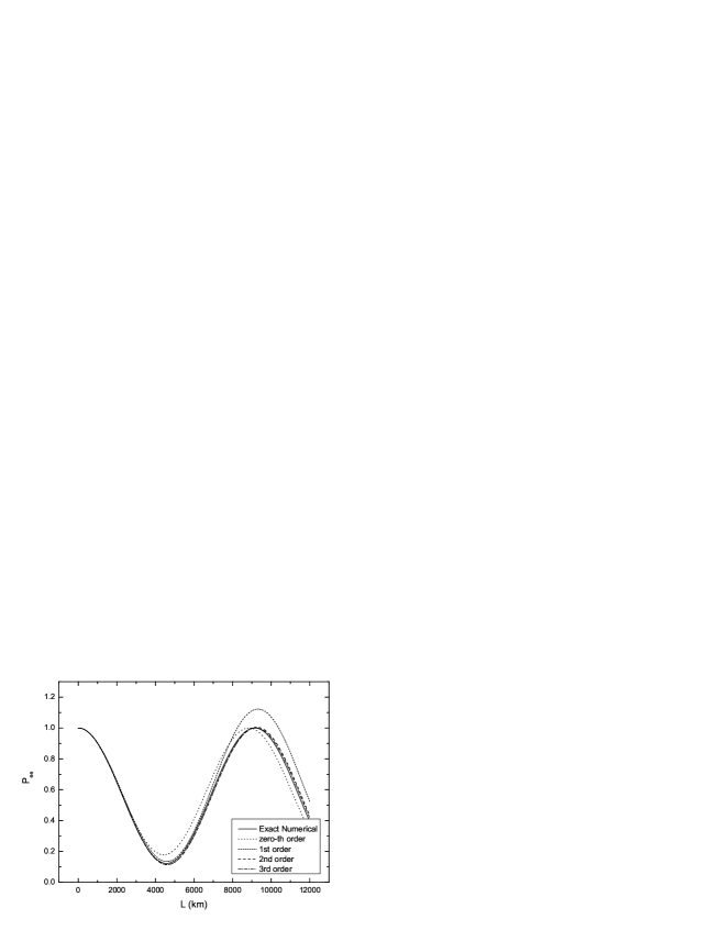
Figure 1: Electron neutrino survival probability as a function of length of baseline $L$ with $E=10MeV$ and $\rho=6.0g/cm^{3}$ ($V\approx 2\times 10^{-13}eV$) and best-fit KamLAND data [22] parameter values: $\Delta m_{sol}^{2}=7.1\times 10^{-5}eV^{2}$ and $\theta_{sol}=32.5^{\circ}$.

Figure 2: Electron neutrino survival probability as a function of energy $E$ with baseline length $L=7400~{}km$ and $\rho=6.0g/cm^{3}$ ($V\approx 2\times 10^{-13}eV$) and best-fit KamLAND data [22] parameter values: $\Delta m_{sol}^{2}=7.1\times 10^{-5}eV^{2}$ and $\theta_{sol}=32.5^{\circ}$.

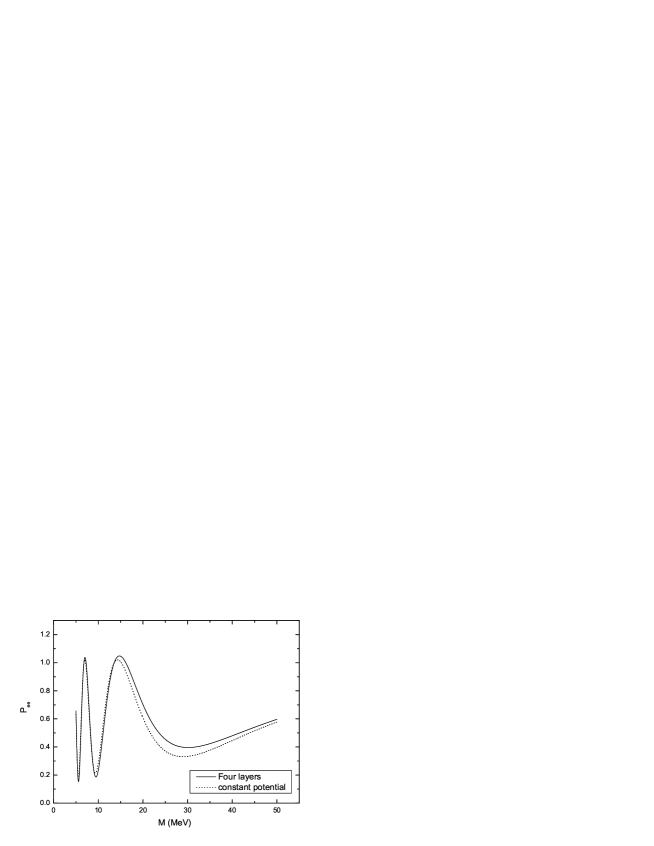
Figure 3: Neutrino oscillation probability $P_{e\rightarrow e}$ vs neutrino energy, when the neutrino flux pass through the center of the Earth with best-fit KamLAND data [22] parameter values: $\Delta m_{sol}^{2}=7.1\times 10^{-5}eV^{2}$ and $\theta_{sol}=32.5^{\circ}$