Magnetism and superconductivity
in quark matter

Abstract

Magnetic properties of quark matter and its relation to the microscopic origin of the magnetic field observed in compact stars are studied. Spontaneous spin polarization appears in high-density region due to the Fock exchange term, which may provide a scenario for the behaviors of magnetars. On the other hand, quark matter becomes unstable to form spin density wave in the moderate density region, where restoration of chiral symmetry plays an important role. Coexistence of magnetism and color superconductivity is also discussed.

1 Introduction

QCD has been believed to be the basic theory of strong interaction and there are many successful consequences about the properties of hadrons and their interactions. Recently many studies have been devoted to figure out the phase diagram of QCD in temperature ($T$) - density ($\rho_{B}$) plane [1, 2]. At high temperature or high density, quarks confined inside hadrons should be liberated to form matter consisting of quarks and gluons (deconfinement transition). Such basic constituents, especially quarks exhibit interesting properties there as electrons in condensed matter through many-body dynamics; one of the interesting possibility is phase transition as temperature or density changes. When we emphasize the low $T$ and high $\rho_{B}$ region, the subjects are sometimes called high-density QCD. The main aims in this field should be to elucidate the new phases and their properties, and to extract their symmetry breaking pattern and low-energy excitation modes there on the basis of QCD. On the other hand, these studies have phenomenological implications on relativistic heavy-ion collisions and compact stars like neutron stars or quark stars [3].

Color superconductivity (CSC) should be very popular [1, 4]. Its mechanism is similar to the BCS theory for the electron-phonon system [5], in which the attractive interaction of electrons is provided by phonon exchange and causes the Cooper instability near the Fermi surface. As for quark matter, the quark-quark interaction is mediated by colored gluons, and is often approximated by some effective interactions, e.g., the one-gluon-exchange (OGE) or the instanton-induced interaction, both of which give rise to the attractive quark-quark interaction in the color anti-symmetric $\bar{3}$ channel. Many people believe that it is robust due to the Cooper instability even for small attractive quark-quark interaction in color $\bar{3}$ channel.

Here we’d like to address another interesting property of quark matter, magnetic properties of quark matter. We shall see various types of magnetic ordering may be expected in quark matter at finite density or temperature. They arise due to the quark particle-hole ($p-h$) correlations in the pseudo-scalar or axial-vector channel.

Phenomenologically the concept of magnetism should be directly related to the origin of strong magnetic field observed in compact stars [6]; e.g., it amounts to $O(10^{12}$G) at the surface of radio pulsars. Recently a new class of pulsars called magnetars has been discovered with super strong magnetic field, $B_{s}\sim 10^{14-15}$G, estimated from the $P-\dot{P}$ curve [7]. First observations are indirect evidences for the superstrong magnetic field, but discoveries of some absorption lines stemming from the cyclotron frequency of protons have been currently reported [8]; when it is confirmed that they originate from protons, they give a direct evidence for the superstrong magnetic field.

Table 1: Surface magnetic field and the radius of stars by the conservation of the magnetic flux.

	$B_{S}[{\rm G}]$	$R[{\rm cm}]$
Sun (obs.)	$10^{3}$	$10^{10}$
Neutron star	$10^{11}$	$10^{6}$
Magnetar	$10^{15}$	$10^{4}$

The origin of the strong magnetic field in compact stars has been a long standing problem since the first discovery of a pulsar [6]. A simple working hypothesis is the conservation of the magnetic flux and its squeezing during the evolution from a main-sequence progenitor star to a compact star; $B\propto R^{-2}$ with $R$ being the radius. Taking the sun as a typical main-sequence star, we have $B\sim 10^{3}$G and $R\sim 10^{10}$cm. If it is squeezed to a typical radius of usual neutron stars, $R\sim 10$km, the conservation of the magnetic flux gives $10^{11}$G, which is consistent with the observations for radio pulsars. However, we find $R\sim 100$m to explain $B\sim 10^{15}$G observed for magnetars, which may lead to a contradiction since the Schwatzschild radius is $O(1$km) for the canonical mass of $O(M_{\odot})$, which is much larger than $R$.

Since dense hadronic matter should be widely developed inside compact stars, it would be reasonable to inquire a microscopic origin of such strong magnetic field: ferromagnetism (FM) or spin polarization is one of the candidates to explain it. Makishima also suggested the hadronic origin of the magnetic field observed in binary X-ray pulsars or radio pulsars[9], since it looks no field decay in these objects.

When we consider the magnetic-interaction energy by a simple formula, $E_{\rm mag}=\mu_{i}B$ with the magnetic moment, $\mu_{i}=e_{i}/(2m_{i})$, we can easily estimate it for $B=O(10^{15}$G) (see Table 2); it amounts to several MeV for electrons, while several keV for nucleons and 10 keV- 1MeV for quarks dependent on their mass.

Table 2: Magnetic interaction energies $E_{\rm mag}$ for $10^{15}$G and the typical energy scales $E_{\rm typ}$ in electron, nucleon and quark systems.

	electron	proton	quark
$m_{i}[{\rm MeV}]$	0.5	$10^{3}$	1- 100
$E_{\rm mag}[{\rm MeV}]$	5 - 6	$2.5\times 10^{-3}$	$2.5\times 10^{-2}-2.5$
$E_{\rm typ}$	keV	MeV	MeV

This simple consideration may imply that strong interaction gives a feasible origin for the strong magnetic field, since its typical energy scale is MeV. The possibility of ferromagnetism in nuclear matter has been elaborately studied since the first discovery of pulsars, but negative results have been reported so far [10]. We consider here its possibility in quark matter as an alternative in light of recent development of high-density QCD [11].

If FM is realized in quark matter, there should be some interplay with CSC; we examine a possibility of the coexistence of FM and CSC in quark matter, where we shall see an interplay between particle-particle and particle-hole correlations. As far as we know, interplay between the color superconducting phase and other phases characterized by the non-vanishing mean fields of the spinor bilinears has not been explored except for the case of chiral symmetry breaking [12].

It would be worth mentioning in this context that ferromagnetism (or spin polarization) and superconductivity are fundamental concepts in condensed matter physics, and their coexistent phase has been discussed and expected for a long time [13]. As a recent progress, superconducting phases have been discovered in some ferromagnetic materials and many efforts have been made to understand the coexisting mechanism [14]. In this phenomenon itinerant electrons may be responsible, while its mechanism is not fully elucidated yet. Many people believe that the electron Cooper pair should be $P-$ wave, since this type can be compatible with spin polarization. We can easily consider the similar situation in quark matter. Since the volumes of the Fermi seas of quarks with different spins result in being different due to the net presence of magnetization, we could not construct a quark Cooper pair in a usual manner as $J^{P}=0^{+}$. Instead, we consider the $J^{P}=0^{-}$ pairing with orbital angular momentum $L=1$ and total spin $S=1$. For the $S=1$ state we further consider two possibilities: spin-parallel pair or spin-anti-parallel pair. We first discuss the former case in detail, which may have a direct resemblance to the electron case. Subsequently we briefly sketch our idea about the former case. Anyway we shall see the gap functions become anisotropic in the momentum space like in ³He or nuclear matter [40, 41].

We discuss another magnetic aspect in quark matter at moderate densities, where the QCD interaction is still strong and some non-perturbative effects still remain. One of the most important phenomena observed there is restoration of chiral symmetry. In the vacuum chiral symmetry is spontaneously broken to give finite mass for quarks or nucleon; we may bear in mind such a picture that the vacuum is in a kind of superconducting phase with massless quark ($q$)-anti-quark ($\bar{q}$) pair condensate, and the gap opened at the top of the Dirac sea corresponds to the finite mass. As a consequence the vacuum does not possess chiral symmetry any more. At finite densities the suppression of $\bar{q}q$ excitations due to the existence of the Fermi sea gives rise to restoration of chiral symmetry at a certain density, and many people believe that deconfinement transition occurs at almost the same density.

There have been proposed various types of the p-h condensations at moderate densities [15, 16], in which the p-h pair in scalar or tensor channel has the finite total momentum indicating standing waves (the chiral density waves). The instability for the density wave in quark matter was first discussed by Deryagin et al. [15] at asymptotically high densities where the interaction is very weak, and they concluded that the density-wave instability prevails over the BCS one in the large $N_{c}$ (the number of colors) limit due to the dynamical suppression of colored BCS pairings.

In general, density waves are favored in 1-D (one spatial dimension) systems and have the wave number $Q=2k_{F}$ according to the Peierls instability [17, 18], e.g., charge density waves (CDW) in quasi-1-D metals [19]. The essence of its mechanism is the nesting of Fermi surfaces and the level repulsion (crossing) of single particle spectra due to the interaction for the finite wave number. Thus the low dimensionality has a essential role to produce the density-wave states. In the higher dimensional systems, however, the transitions occur provided the interaction of a corresponding (p-h) channel is strong enough. For the 3-D electron gas, it was shown by Overhauser [20, 21] that paramagnetic state is unstable with respect to the formation of the static spin density wave (SDW), in which spectra of up- and down-spin states are deformed to bring about the level crossing due to the Fock exchange interactions, while the wave number does not precisely coincide with $2k_{F}$ because of the incomplete nesting in higher dimension.

We shall see a kind of spin density wave develops there, in analogy with SDW mentioned above.. It occurs along with the chiral condensation and is represented by a dual standing wave in scalar and pseudo-scalar condensates (we have called it ‘dual chiral-density wave’, DCDW). DCDW has different features in comparison with the previously discussed chiral density waves [15, 16]. One outstanding feature concerns its magnetic aspect; DCDW induces spin density wave.

2 Ferromagnetism in QCD

2.1 A heuristic argument

Quark matter bears some resemblance to electron gas interacting with the Coulomb potential; the one gluon exchange (OGE) interaction in QCD has some resemblance to the Coulomb interaction in QED , and color neutrality of quark matter corresponds to total charge neutrality of electron gas under the background of positively charged ions.

It was Bloch who first suggested a mechanism leading to ferromagnetism of itinerant electrons within the Hartree-Fock approximation [22]. The mechanism looks very simple but largely reflects the Fermion nature of electrons in a model-independent way. Since there works no direct interaction between charged particles as a whole, the Fock exchange interaction gives a leading contribution. Then it is immediately conceivable that a most attractive channel is the parallel spin pair, whereas the anti-parallel pair gives null contribution (see Eq. (8) below). This is nothing but a consequence of the Pauli exclusion principle: electrons with the same spin cannot closely approach to each other, which efficiently avoid the Coulomb repulsion. Thus a completely polarized state is favored by the interaction. On the other hand a polarized state should have a larger kinetic energy by rearranging the two Fermi spheres. Thus there is a trade-off between the kinetic and interaction energies, which leads to a spontaneous spin polarization (SSP) or FM at a certain density. Subsequently it has been proved that Bloch’s idea is qualitatively justified, but the critical density can not be reliably estimated without examining the higher-order correlation diagrams [23, 24]; especially the ring diagrams have been known to be important in the calculation of the susceptibility of electron gas. Recently the possibility of ferromagnetism in the electron gas has been studied by the quantum Monte Carlo simulation and it has been shown that the electron gas is in ferromagnetic phase at very low electron density [25]. Authors in ref.[26] have confirmed it experimentally.

One of the essential points we learned here is that we need no spin-dependent interaction in the original Lagrangian to see SSP: a symmetry principle gives rise to a spin dependent interaction.

Then it might be natural to ask how about in QCD. We list here some features of QCD related to this subject. (1) the quark-gluon interaction in QCD is rather simple, compared with the nuclear force; it is a gauge interaction like in QED. (2) quark matter should be a color neutral system and only the $\it Fock~{}exchange$ interaction is also relevant like in the electron system. (3) there is an additional flavor degree of freedom in quark matter; gluon exchange never change flavor but it becomes effective through the generalized Pauli principle. (4) quarks should be treated relativistically, different from the electron system.

The last feature requires a new definition and formulation of SSP or FM in relativistic systems since “spin” is no more a good quantum number for relativistic particles; spin couples with momentum and its direction changes during the motion. It is well known that the Pauli-Lubanski vector $W^{\mu}$ is the four vector to represent the spin degree of freedom in a covariant form; the spinor of the free Dirac equation is the eigenstate of the operator,

$$W\cdot a=-\frac{1}{2}\gamma_{5}a/k/,$$ (1)

where a 4-axial-vector $a^{\mu}$ is orthogonal to $k$ s.t.

$${\bf a}=\mbox{\boldmath$\zeta$}+\frac{{\bf k}(\mbox{\boldmath$\zeta$}\cdot{\bf k})}{m(E_{k}+m)},~{}a^{0}=\frac{{\bf k}\cdot\mbox{\boldmath$\zeta$}}{m}~{}~{}~{}$$ (2)

with the axial vector $\zeta$. We can see that $a^{\mu}$ is reduced to a three vector $(0,\mbox{\boldmath$\zeta$})$ in the rest frame, where we can allocate $\mbox{\boldmath$\zeta$}=(0,0,\pm 1)$ to spin “up” and “down” states. Thus we can still use $\zeta$ to specify the two intrinsic polarized states even in the general Lorentz frame. To characterize the degeneracy of the plane wave solution $u^{(\alpha)}(k)$ ($\alpha=1,2$) for a positive energy state, we can use such spinors $u^{(\alpha)}(k)$ that are eigenstates of the operator $-W\cdot a/m_{q}$: for the standard representation of $u^{(\alpha)}(k)$ [27],

$$-\frac{W\cdot a}{m_{q}}u^{(\alpha)}(k)=\pm\frac{1}{2}u^{(\alpha)}(k).$$ (3)

Accordingly, the polarization density matrix $\rho(k,\mbox{\boldmath$\zeta$})$ is given by the expression,

$$\rho(k,\mbox{\boldmath$\zeta$})=\frac{1}{2m_{q}}(k/+m_{q})P(a),\quad P(a)=\frac{1}{2}(1+\gamma_{5}a/),$$ (4)

which is normalized by the condition, ${\rm tr}\rho(k,\mbox{\boldmath$\zeta$})=1$ [28].

Consider the spin-polarized quark liquid with the total number density of quarks $n_{q}$ ; we denote the number densities of quarks with spin up and down by $n_{+}$ and $n_{-}$, respectively , and introduce the polarization parameter $p$ by the equations, $n_{\pm}=\frac{1}{2}n_{q}(1\pm p),$ under the condition $0\leq p\leq 1$. We assume as usual that three color states are occupied to be neutral for each momentum and spin state. The Fermi momenta in the spin-polarized quark matter are then $k_{F}^{\pm}=k_{F}(1\pm p)^{1/3}$ with $k_{F}=(\pi^{2}n_{q})^{1/3}$. The kinetic energy density is given by the standard formula,

$$\epsilon_{kin}=\frac{3}{16\pi^{2}}\sum_{i=\pm}\left[k_{F}^{i}E_{F}^{i}(2k_{F}^{i2}+m^{2}_{q})-m^{4}_{q}\ln\left(\frac{E_{F}^{i}+k_{F}^{i}}{m_{q}}\right)\right],$$ (5)

with the Fermi energy $E_{F}^{i}=(m^{2}_{q}+k_{F}^{i2})^{1/2}$.

Let us consider the OGE interaction between two quarks with momenta, $k$ and $q$, and spin vectors, $\zeta$ and $\mbox{\boldmath$\zeta$}^{\prime}$, respectively. The color symmetric matrix element ${\cal M}^{s}_{{\bf k}\zeta,{\bf q}\zeta^{\prime}}$ is given only by the exchange term; the direct term vanishes because the color symmetric combinations ($\sim{\rm tr}\lambda_{a}$) does not couple to gluons. Thus

$${\cal M}^{s}_{{\bf k}\zeta,{\bf q}\zeta^{\prime}} = -g^{2}\frac{1}{9}{\rm tr}(\lambda_{a}/2\lambda_{a}/2)\bar{u}^{(\zeta^{\prime})}({\bf q})\gamma_{\mu}u^{(\zeta)}({\bf p})\bar{u}^{(\zeta)}({\bf p})\gamma^{\mu}u^{(\zeta^{\prime})}({\bf q})\frac{-1}{(k-q)^{2}}$$ (6)

$$= \frac{4}{9}g^{2}\frac{1}{4}{\rm tr}\left[\gamma_{\mu}\rho(k,\zeta)\gamma^{\mu}\rho(q,\zeta^{\prime})\right]\frac{1}{(k-q)^{2}},$$

by the use of Eq. (4). If we choose both $\zeta$ and $\mbox{\boldmath$\zeta$}^{\prime}$ in parallel along the $z$ axis, $\mbox{\boldmath$\zeta$}=\mbox{\boldmath$\zeta$}^{\prime}=(0,0,\pm 1)$, we have the spin-nonflip amplitude ${\cal M}^{s,nonflip}_{{\bf p}{\bf q}}$, while if we choose them in anti-parallel, $\mbox{\boldmath$\zeta$}=-\mbox{\boldmath$\zeta$}^{\prime}$, we have the spin-flip amplitude ${\cal M}^{s,flip}_{{\bf p}{\bf q}}$. Each form of the spin-nonflip or spin-flip amplitude is complicated, but their average gives a simple form,

$$\overline{{\cal M}}^{s}_{{\bf p}{\bf q}}=\frac{2}{9}g^{2}\frac{2m^{2}_{q}-k\cdot q}{(k-q)^{2}},$$ (7)

which is nothing but the matrix element for the unpolarized case [29]. In the nonrelativistic limit, $m_{q}\gg|{\bf p}|,|{\bf q}|$, the matrix element is reduced to the form,

$${\cal M}^{s}_{{\bf k}\zeta,{\bf q}\zeta^{\prime}}=-\frac{2}{9}g^{2}\frac{m_{q}^{2}(1+\mbox{\boldmath$\zeta$}\cdot\mbox{\boldmath$\zeta$}^{\prime})}{|{\bf k}-{\bf q}|^{2}},$$ (8)

so that there is no correlation between quarks with different spins. On the other hand, there is some correlation included in the relativistic case.

After summing up over the color degree of freedom and performing the integrals of the color symmetric matrix element ${\cal M}^{s}_{{\bf k}\zeta,{\bf q}\zeta^{\prime}}$ over the Fermi seas of spin up and down quarks, we have the exchange energy density $\epsilon_{ex}$ consisting of two contributions,

$$\epsilon_{ex}=\epsilon_{ex}^{nonflip}+\epsilon_{ex}^{flip}.$$ (9)

In the nonrelativistic case, the spin-flip contribution becomes tiny and the dominant contribution for the OGE energy density in Eq.(9) comes from the spin-nonflip contribution (see Eq. (8)),

$$\epsilon_{ex}\sim-\frac{\alpha_{c}k_{F}^{4}}{2\pi^{3}}\left\{(1+p)^{4/3}+(1-p)^{4/3}\right\}.$$ (10)

The exchange energy is negative and takes a minimum at $p=1$. The form of the energy density (10) is exactly the same as in electron gas. It is the difference of density dependence between the contributions given in Eqs. (5) and (10) which causes a ferromagnetic instability; this mechanism was first pointed out by Bloch for electron gas [22].

In the relativistic case there are some different features from the nonrelativistic case. First, there is a spin-flip contribution due to the lower component of the Dirac spinor even for the Coulomb-like interaction. Secondly, the transverse (magnetic) gluons becomes important, where the spin-flip effect is prominent. Finally, the density dependence of kinetic energy as well as the exchange energy is very different [31]. Before discussing the general case, we consider the relativistic limit, $k_{F}^{i}\gg m_{q}$; the Fock exchange-energy density looks like

$$\epsilon_{ex}\sim\frac{\alpha_{c}}{8\pi^{3}}k_{F}^{4}\left\{(1+p)^{4/3}+(1-p)^{4/3}+2(1-p^{2})^{2/3}\right\},$$ (11)

which is a decreasing function and takes a minimum again at $p=1$. This is due to the characteristic feature of the spin-flip and spin-nonflip interactions: both give a repulsive contribution in the relativistic limit and there is no spin-flip interaction in the polarized state ($p=1$). Thus, ferromagnetism in the relativistic limit arises by a different mechanism from that in the nonrelativistic case.

In Fig.1 a typical shape of the total energy density, $\epsilon_{tot}=\epsilon_{kin}+\epsilon_{ex}$, is depicted as a function of the polarisation parameter $p$, e.g. for the parameter set ,$m_{q}=300$MeV of the $s$ quark and $\alpha_{c}=2.2$ as in the MIT bag model [32] . We can see that paramagnetic quark matter ($p=0$) becomes unastable as density decreases, and ferromagnetic phase is favored at a certain density between 0.1 and 0.2 fm^-3. This phase transition is of weakly first-order and the completely polarized ($p=1$) state appears at the critical density.

Figure 1: First-order phase transition to the ferromagnetic state.

Figure 2: Critical lines as functions of quark-number density.

To figure out the features of the ferromagnetic transition, we study other quantities. For small $p\ll 1$, the energy density behaves like

$$\epsilon_{tot}-\epsilon_{tot}(p=0)=\chi^{-1}p^{2}+O(p^{4})$$ (12)

with $\chi^{-1}\equiv\chi_{kin}^{-1}+\chi_{ex}^{-1}$. $\chi$ is proportional to the magnetic susceptibility, and its sign change indicates a ferromagnetic transition, if it is of the second order. It consists of two contributions: the kinetic energy gives $\chi_{kin}^{-1}=k_{F}^{5}/(3\pi^{2}E_{F})$ (c.f. the Pauli paramagnetism), which changes from $\chi_{kin}^{-1}\sim O(k_{F}^{5})$ at low densities to $\chi_{kin}^{-1}\sim O(k_{F}^{4})$ at high densities. On the other hand, the Fock exchange energy gives

$$\chi_{ex}^{-1}=-\frac{2\alpha_{c}k_{F}^{4}}{9\pi^{3}}\left[2-\frac{k_{F}^{2}}{E_{F}^{2}}-\frac{3m_{q}^{2}k_{F}}{E_{F}^{3}}\ln\left(\frac{E_{F}+k_{F}}{m_{q}}\right)+\frac{4m_{q}k_{F}^{2}}{3E_{F}^{2}(E_{F}+m_{q})}\right]$$ (13)

[30], which is reduced to

$$\chi_{ex}^{-1}\sim-\frac{4\alpha_{c}}{9\pi^{3}}k_{F}^{4}$$ (14)

in the nonrelativistic limit, $p_{F}\ll m_{q}$. In the relativistic limit, $p_{F}\gg m_{q}$, it behaves like

$$\chi_{ex}^{-1}\sim\frac{\alpha_{c}}{9\pi^{3}}k_{F}^{4}-\frac{\alpha_{c}}{3\pi^{3}}k_{F}^{4}=-\frac{2\alpha_{c}}{9\pi^{3}}k_{F}^{4},$$ (15)

where the first term stems from the spin-nonflip contribution, while the second term from the spin-flip contribution. Then we can see that the effect of the spin-flip contribution overwhelms the one of the spin-nonflip contribution. The interaction contribution $\chi_{ex}^{-1}$ is always negative , and dominant over $\chi_{kin}^{-1}$ at low densities, while the kinetic contribution $\chi_{kin}$ is always positive. If $\alpha_{c}>3\pi/2=4.7$, $\chi$ becomes negative over all densities.

For a given set of $m_{q}$ and $\alpha_{c}$, $\chi$ changes its sign at a certain density, denoted by $n_{c1}$, and it is a signal for the second-order phase transition. Note that the ferromagnetic transition in our case is of the first order, so that it is not sufficient to only see the magnetic susceptibility; even above that density the ferromagnetic phase may be possible. Actually there is a range, $n_{c1}<n_{q}<n_{c2}$, where $\chi>0$ but $\epsilon<0$.

Above the density $n_{c2}$ there is no longer the stable ferromagnetic phase. However, the metastable state is still possible up to the density $n_{c3}$, which is specified by the condition s.t. $\eta\equiv\partial\epsilon_{tot}/\partial p~{}|_{p=1}<0$. In Fig.2 we depict the quantities $\chi^{-1},\delta\epsilon$ and $\eta$ as the functions of density, e.g. for the set ,$m_{q}=300$MeV and $\alpha_{c}=2.2$. The crossing points with the horizontal axis indicate the critical deisities $n_{c1},n_{c2}$ and $n_{c3}$, respectively. We can see that the ferromagnetic instability occurs at low densities, while the metastable state can exist up to rather high densities.

Finally we show the critical lines satisfying $\chi^{-1}=0,\delta\epsilon=0$ and $\eta=0$ in the QCD parameter ($\alpha_{c}$ and $m_{q}$) plane, which seperate the three characteristic regions for a given density. In Fig. 3 we demonstrate them at a density $n_{q}=0.3$fm^-3. All the lines have the maxima around the medium quark mass, and the mechanism of ferromagnetism is different for each side of the maximum, as already discussed. If we take $m_{q}=300$MeV for the $s$ quark or $m_{q}\sim 0$MeV for the $u$ or $d$ quark, and $\alpha_{c}=2.2$ as in the MIT bag model again [32], the quark liquid can be ferromagnetic as a metastable state.

Figure 3: Phase diagram in the coupling-strength ($\alpha_{s}$)-mass ($m_{q}$) plane.

We have seen that the ferromagnetic phase is realized at low densities and the metastable state is plausible up to rather high densities for a reasonable range of the QCD parameters. Our calculation is based on the lowest-order perturbation. So we need to examine the higher-order gluon-exchange contributions to confirm the possibility. It should be interesting to refer a recent paper [34], where the author also found the ferromagnetic transition at low densities within the perturbative QCD calculation beyond the lowest-order diagram.

If a ferromagnetic quark liquid exists stably or metastably around or above nuclear density, it has some implications on the properties of strange quark stars and strange quark nuggets [35]. They should be magnetized in a macroscopic scale. Considering a possibility to attribute magnetars to strange quark stars in a ferromagnetic phase, we roughly estimate the strength of the magnetic field at the surface of a strange quark star. Taking the stellar parameters of strange quark stars to be similar to those for canonical neutron stars with the typical mass around $M_{G}=1.4M_{\odot}$, we find the total magnetic dipole moment $M_{q}$, $M_{q}=\mu_{q}\cdot(4\pi/3\cdot r_{q}^{3})n_{q}$ for the quark sphere with the density $n_{q}$ and the radius $r_{q}$, where $\mu_{q}$ is the magnetic moment of each quark. Then the dipolar magnetic field at the star surface $r=R\simeq 10$km takes a maximal strength at the poles,

$$B_{\rm max}=\frac{8\pi}{3}\left(\frac{r_{q}}{R}\right)^{3}\mu_{q}n_{q}=10^{15}[{\rm G}]\left(\frac{r_{q}}{R}\right)^{3}\left(\frac{\mu_{q}}{\mu_{N}}\right)\left(\frac{n_{q}}{0.1{\rm fm}^{-3}}\right)$$ (16)

with nuclear magneton $\mu_{N}$, which looks enough for magnetars.

2.2 Self-consistent calculation

If we understand FM or magnetic properties of quark matter more deeply, we must proceeds to a self-consistent approach, like the Hartree-Fock theory, beyond the previous perturbative argument .

We begin with an OGE action:

$$I_{int}=-g^{2}\frac{1}{2}\int{\rm d^{4}}x\int{\rm d^{4}}y\left[\bar{\psi}(x)\gamma^{\mu}\frac{\lambda_{a}}{2}\psi(x)\right]D_{\mu\nu}(x,y)\left[\bar{\psi}(y)\gamma^{\nu}\frac{\lambda_{a}}{2}\psi(y)\right],$$ (17)

where $D^{\mu\nu}$ denotes the gluon propagator. By way of the mean-field approximation, we have

$$I_{MF}=\int\frac{{\rm d}^{4}p}{(2\pi)^{4}}\bar{\psi}(p)G_{A}^{-1}(p)\psi(p).$$ (18)

The inverse quark Green function $G_{A}^{-1}(p)$ involves various self-energy (mean-field) terms, of which we only keep the color singlet particle-hole mean-field $V(p)$,

$$G_{A}(p)^{-1}=/{\!\!\!}{p}-m+/{\!\!\!}{\mu}+V(p).$$ (19)

Taking into account the lowest diagram, we can then write down the self-consistent equations for the mean-field, $V$:

$$-V(k)=(-ig)^{2}\int\frac{{\rm d}^{4}p}{i(2\pi)^{4}}\{-iD^{\mu\nu}(k-p)\}\underbrace{\gamma_{\mu}\frac{\lambda_{\alpha}}{2}\{-iG_{A}(p)\}\gamma_{\nu}\frac{\lambda_{\alpha}}{2}}_{(A)}.$$ (20)

Applying the Fierz transformation for the OGE action (17) we can see that there appear the color-singlet scalar, pseudo-scalar, vector and axial-vector self-energies by the Fock exchange interaction. Taking the Feynman gauge for the gluon propagator, a manupilation gives

$$(A)\!\!\! = \!\!\!\frac{N_{c}^{2}-1}{4N_{c}^{2}}\frac{1}{N_{f}}\!\!\left\{{\rm Tr}(G_{A})\!+\!i\gamma_{5}{\rm Tr}(G_{A}i\gamma_{5})\!-\!\frac{1}{2}[\gamma^{\mu}{\rm Tr}(G_{A}\gamma_{\mu})\!+\!\gamma_{5}\gamma^{\mu}{\rm Tr}(G_{A}\gamma_{5}\gamma_{\mu})]\!\!\right\}$$ (21)

$$+ \{{\rm color~{}non\!{\rm-}\!singlet~{}or~{}flavor~{}non\!{\rm-}\!singlet~{}terms}\}.$$

When we restrict the ground state to be an eigenstate with respect to color and flavor, there is only left the first term which is color singlet and flavor singlet. Still we must take into account various mean-fields in $V$, $V=U_{s}+i\gamma_{5}U_{ps}+\gamma_{\mu}U_{v}^{\mu}+\gamma_{\mu}\gamma_{5}U_{av}^{\mu}$ with the mean-fields $U_{i}$. Here we only retain ${\bf U}_{av}(\equiv{\bf U}_{A})$ for simplicity and suppose that others to be vanished;

$$V(k)=\mbox{\boldmath$\gamma$}\gamma_{5}\cdot{\bf U}_{A}({\bf k}),$$ (22)

with the static axial-vector mean-field $U_{A}({\bf k})$.

The poles of $G_{A}(p)$, $\det$$G^{-1}_{A}$($p_{0}+\mu$$=$$\epsilon_{n}$)$=$$0$, give the single-particle energy spectrum:

$$\epsilon_{n}=\pm\epsilon_{\pm}$$ (23)

$$\epsilon_{\pm}({\bf p})=\sqrt{{\bf p}^{2}+{\bf U}_{A}^{2}({\bf p})+m^{2}\pm 2\sqrt{m^{2}{\bf U}_{A}^{2}({\bf p})+({\bf p}\cdot{\bf U}_{A}({\bf p}))^{2}}},$$ (24)

where the subscript in $\epsilon_{s}({\bf p}),s=\pm$ represents spin degrees of freedom, and the dissolution of the degeneracy corresponds to the exchange splitting of different “spin” states; the spectrum is reduced to a familiar form $\epsilon_{\pm}\sim m+\frac{p^{2}}{2m}\pm|{\bf U}_{A}|$ in the non-relativistic limit [23].

There appear two Fermi seas with different volumes for a given quark number due to the exchange splitting in the energy spectrum. The appearance of the rotation symmetry breaking term, $\propto{\bf p}\cdot{\bf U}_{A}$ in the energy spectrum implies deformation of the Fermi sea: thus rotation symmetry is violated in the momentum space as well as the coordinate space, $O(3)\rightarrow O(2)$. Accordingly the Fermi sea of majority quarks exhibits a “prolate” shape ($F^{-}$), while that of minority quarks an “oblate” shape ($F^{+}$) as seen in Fig. 4.

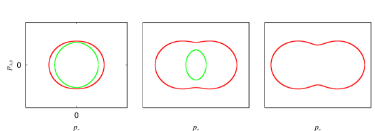
Figure 4: Modification of the Fermi sea as $U_{A}$(=const.) is increased from left to right. The larger Fermi sea ($F^{-}$) takes a prolate shape, while the smaller one ($F^{+}$) an oblate shape for a given $U_{A}$. In the large $U_{A}$ limit (completely polarized case), $F^{+}$ disappears as in the right panel.

Then the self-consistent equation (20) is reduced to the form,

$$U_{A}({\bf k})=\frac{N_{c}^{2}-1}{4N_{c}}{g}^{2}\int\frac{{\rm d}^{3}p}{(2\pi)^{3}}\sum_{s=\pm}\frac{1}{\epsilon_{s}(\mbox{\boldmath$p$})^{2}-|{\bf k}-{\bf p}|^{2}}\theta(\mu-\epsilon_{s}(\mbox{\boldmath$p$}))\frac{U_{A}({\bf p})+s\beta_{p}}{\epsilon_{s}(\mbox{\boldmath$p$})}$$ (25)

with $\beta_{p}=\sqrt{p_{z}^{2}+m^{2}}$ by taking ${\bf U}_{A}$ along the $z$ axis. Here we have discarded the contribution of the Dirac seas and only taken into account that of the Fermi seas.

In the following we demonstrate some numerical results by replacing the original OGE by the “contact” (zero-range) interaction, $D^{\mu\nu}\rightarrow-g^{\mu\nu}/\Lambda^{2},$ which may correspond to the Stoner model in the condensed matter physics [23].

We can easily see that the mean-field $U_{A}$ becomes then momentum-independent, and the expression for $U_{A}$, Eq. (25), is proportional to the simple sum of the expectation value of the spin operator over the Fermi seas;

$${\bar{s}_{z}}=\frac{1}{2}\langle\Sigma_{z}\rangle = -i\int_{C}\frac{d^{4}p}{(2\pi)^{4}}{\rm tr}\gamma_{5}\gamma_{3}G_{A}(p)$$ (26)

$$= \frac{1}{2}\left[\int_{F^{+}}\frac{d^{3}p}{(2\pi)^{3}}\frac{U_{A}({\bf p})+\beta_{p}}{\epsilon_{+}({\bf p})}+\int_{F^{-}}\frac{d^{3}p}{(2\pi)^{3}}\frac{U_{A}({\bf p})-\beta_{p}}{\epsilon_{-}({\bf p})}\right].$$

2.3 Phase diagram on the temperature-density plane

We will present the phase diagram in the three-flavor case under two conditions [37]: the chemical equilibrium condition (CEC) $\mu_{u}=\mu_{d}=\mu_{s}$ and the charge neutral condition without electrons (CNC) $\rho_{u}=\rho_{d}=\rho_{s}$, where quark masses are taken as $m_{u}=m_{d}=5$MeV and $m_{s}=150-350$MeV, i.e., $\mu_{s}=\sqrt{\mu_{u,d}^{2}+m_{s}^{2}-m_{u,d}^{2}}$ for $T=0$. In both conditions, since the spin polarization caused by the axial-vector mean-field is fully enhanced by the quark mass for given density or temperature, choice of the current quark mass seriously affects the results; especially, largeness of the strange quark mass has an essential effect on spin polarization. To get the phase diagram or critical line on the temperature-density plane, we use the thermodynamic potential $\Omega$ within the mean-field approximation,

$$\Omega = -N_{c}\sum_{B=\pm 1}~{}\sum_{s=\pm}~{}\sum_{i=u,d,s}\int\frac{{\rm d}^{3}{\bf k}}{(2\pi)^{3}}T\log\left\{\exp\left[-\frac{\epsilon_{s}({\bf k},m_{i},U_{A})-B\mu_{i}}{T}\right]+1\right\}$$ (27)

$$-N_{c}\sum_{s=\pm}~{}\sum_{i=u,d,s}\int\frac{{\rm d}^{3}{\bf k}}{(2\pi)^{3}}\epsilon_{s}({\bf k},m_{i},U_{A})+\frac{U_{A}^{2}}{4\tilde{g}^{2}},$$

where we have used the “contact” interaction, $\tilde{g}^{2}\equiv g^{2}/\Lambda^{2}$, in place of the OGE interaction. Note that we take into accout the vacuum contribution in this formula (the second term in Eq. (27)), which should be regularized by ,e.g., the proper-time method (see §4.3). We can confirm that the thermodynamic potential reproduces the self-consistent equation for the order parameter $U_{A}$ Eq. (25) in the three-flavor case, except the vacuum contribution. The vacuum (the Dirac sea) contribution always works against spin polarization as it should do, while the contribution of the Fermi sea gives rise to spontaneous spin polarization.

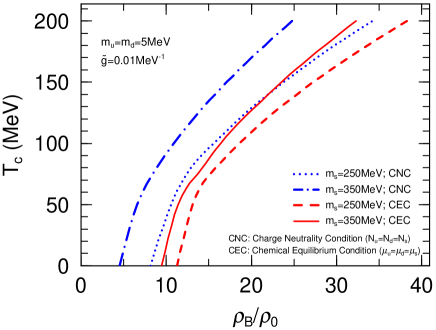
Figure 5: Phase diagram for two cases of strange quark masses, $250,350$MeV.

Fig. 5 shows the critical temperature (the Curie temperature) as a function of baryon-number density under the two conditions mentioned above; CEC and CNC. We can see that CNC tends to facilitate the system having spin polarization than CEC. This is because CNC holds the larger strange-quark density than CEC.

Since the axial-vector mean-field arises from the Fock exchange interaction among quarks in the Fermi sea and causes a kind of particle-hole condensation, there exists a critical density for a given coupling constant $\tilde{g}$. We show the critical density by varying the effective coupling constant $\tilde{g}$ in Fig. 6.

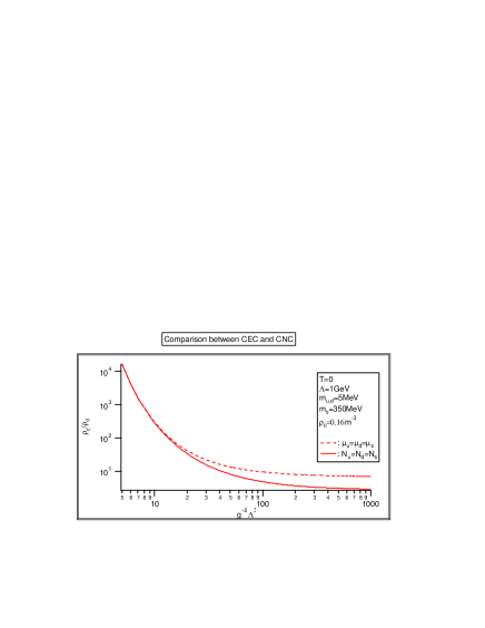
Figure 6: Critical density as a function of $\tilde{g}$ under two conditions: CEC and CNC.

The critical density is more lowered with the larger coupling strength, and this tendency is remarkable in the case of CNC. The result also indicates that even for the weak-coupling regime in QCD, spin polarization may appear at sufficiently large densities and low temperatures.

3 Color magnetic superconductivity

3.1 General framework

If FM is realized in quark matter, it might be in the CSC phase. In this section we discuss a possibility of the coexistence of FM and CSC, which we call Color magnetic superconductivity [38].

Recall the OGE action Eq. (17). By way of the mean-field approximation, we have

$$I_{MF}=\frac{1}{2}\int\frac{{\rm d}^{4}p}{(2\pi)^{4}}\left(\begin{array}[]{l}\bar{\psi}(p)\\ \bar{\psi}_{c}(p)\\ \end{array}\right)^{T}G^{-1}(p)\left(\begin{array}[]{l}\psi(p)\\ \psi_{c}(p)\\ \end{array}\right)\\$$ (28)

in the Nambu-Gorkov formalism, allowing not only the particle-hole but also the particle-particle mean-field. The inverse quark Green function $G^{-1}(p)$ involves various self-energy (mean-field) terms, of which we only keep the color singlet particle-hole $V(p)$ and color $\bar{3}$ particle-particle ($\Delta$) mean-fields; the former is responsible to ferromagnetism, while the latter to superconductivity,

$$G^{-1}(p) = \left(\begin{array}[]{cc}/{\!\!\!}{p}-m+/{\!\!\!}{\mu}+V(p)&\gamma_{0}\Delta^{\dagger}(p)\gamma_{0}\\ \Delta(p)&/{\!\!\!}{p}-m-/{\!\!\!}{\mu}+\overline{V}(p)\\ \end{array}\right),$$ (31)

$$= \left(\begin{array}[]{cc}G_{11}(p)&G_{12}(p)\\ G_{21}(p)&G_{22}(p)\\ \end{array}\right)^{-1}$$ (34)

where

$$\psi_{c}(k)=C\bar{\psi}^{T}(-k),~{}~{}~{}\overline{V}\equiv CV^{T}C^{-1}.$$ (35)

Taking into account the lowest diagram, we can then write down the self-consistent equations for the mean-fields, $V$ and $\Delta$:

$$-V(k)=(-ig)^{2}\int\frac{{\rm d}^{4}p}{i(2\pi)^{4}}\{-iD^{\mu\nu}(k-p)\}\gamma_{\mu}\frac{\lambda_{\alpha}}{2}\{-iG_{11}(p)\}\gamma_{\nu}\frac{\lambda_{\alpha}}{2}.$$ (36)

and

$$-\Delta(k)=(-ig)^{2}\int\frac{{\rm d}^{4}p}{i(2\pi)^{4}}\{-iD^{\mu\nu}(k-p)\}\gamma_{\mu}\frac{-(\lambda_{\alpha})^{T}}{2}\{-iG_{21}(p)\}\gamma_{\nu}\frac{\lambda_{\alpha}}{2},$$ (37)

(c.f. Eq. (20)).

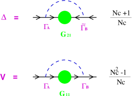
Figure 7: Graphical interpretations of the coupled equations (36) and (37) with coefficients in front of R.H.S. given by $N_{c}$. The lower diagram becomes dominant in the large $N_{c}$ limit.

The structure of Eq. (36) is the same as Eq. (20), and we can see there appear the color-singlet scalar, pseudoscalar, vector and axial-vector self-energies by applying the Fierz transformation . Here we retain only $U_{s},U_{v}^{0},U_{av}^{3}$ in $V$ and suppose that others to be vanished as before. We shall see this ansatz gives self-consistent solutions for Eq.(36) within the zero-range approximation for the OGE interaction because of axial and reflection symmetries of the Fermi seas. We furthermore discard the scalar mean-field $U_{s}$ and the time component of the vector mean-field $U_{v}^{0}$ for simplicity since they are irrelevant for the spin degree of freedom.

According to the above assumptions and considerations the mean-field $V$ in Eq.(34) renders

$$V=\gamma_{3}\gamma_{5}U_{A},~{}~{}~{}U_{A}\equiv U_{av}^{3},$$ (38)

with the axial-vector mean-field $U_{A}$, as in Eq. (22). Then the diagonal component of the Green function $G_{11}(p)$ is written as

$$G_{11}(p)=\left[G_{A}^{-1}-\gamma_{0}\Delta^{\dagger}\gamma_{0}\tilde{G}_{A}\Delta\right]^{-1}$$ (39)

with

$$G_{A}^{-1}(p) = /{\!\!\!}{p}-m+/{\!\!\!}{\mu}-\gamma_{5}\gamma_{3}U_{A},$$ (40)

$$\tilde{G}_{A}^{-1}(p) = /{\!\!\!}{p}-m-/{\!\!\!}{\mu}-\overline{\gamma_{5}\gamma_{3}}U_{A},$$ (41)

where $\overline{\gamma_{5}\gamma_{3}}=\gamma_{5}\gamma_{3}$ and $G_{A}(p)$ is the Green function with $U_{A}$ which is determined self-consistently by way of Eq. (20).

3.2 ${}^{3}P$ type anisotropic pairing

Before constructing the gap function $\Delta$, we first find the single-particle spectrum and their eigenspinors in the absence of $\Delta$, which is achieved by diagonalization of the operator $G_{A}^{-1}$. We have already known four single-particle energies $\epsilon_{\pm}$ (positive energies) and $-\epsilon_{\pm}$ (negative energies), which are given as

$$\epsilon_{\pm}({\mbox{\boldmath$p$}})=\sqrt{{\mbox{\boldmath$p$}}^{2}+U_{A}^{2}+m^{2}\pm 2U_{A}\sqrt{m^{2}+p_{z}^{2}}},$$ (42)

and the eigenspinors $\phi_{s},~{}s=\pm$ should satisfy the equation, $G_{A}^{-1}(\epsilon_{s},{\bf p})\phi_{s}=0$.

Here we take the following ansatz for $\Delta$:

$$\Delta({\mbox{\boldmath$p$}}) = \sum_{s=\pm}\tilde{\Delta}_{s}({\mbox{\boldmath$p$}})B_{s}({\mbox{\boldmath$p$}}),$$

$$B_{s}({\mbox{\boldmath$p$}}) = \gamma_{0}\phi_{-s}({\mbox{\boldmath$p$}})\phi_{s}^{\dagger}({\mbox{\boldmath$p$}}).$$ (43)

The structure of the gap function (43) is then inspired by a physical consideration of a quark pair as in the usual BCS theory: we consider here the quark pair on each Fermi surface with opposite momenta, ${\bf p}$ and $-{\bf p}$ so that they result in a linear combination of $J^{\pi}=0^{-},1^{-}$ (see Fig. 9) .

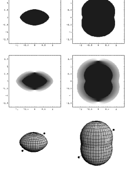
Figure 8: Deformed Fermi seas and the quark pair on each surface. The top figures show those in the absence of $\Delta_{\pm}$ and the middle figures diffusion of the Fermi surfaces in the presence of $\Delta_{\pm}$. The bottom ones show the quark pairing on the Fermi surfaces.

Figure 9: Schematic view of the polar-angle dependence of the gap functions at the Fermi surface, (a) for $m=0$ and (b) for $m\neq 0$.

$\tilde{\Delta}_{s}$ is still a matrix in the color-flavor space. Since the anti-symmetric nature of the fermion self-energy imposes a constraint on the gap function [4],

$$C\Delta({\mbox{\boldmath$p$}})C^{-1}=\Delta^{T}({-\mbox{\boldmath$p$}}).$$ (44)

$\tilde{\Delta}_{n}({\mbox{\boldmath$p$}})$ must be a symmetric matrix in the spaces of internal degrees of freedom. Taking into account the property that the most attractive channel of the OGE interaction is the color anti-symmetric ${\bar{3}}$ state, it must be in the flavor singlet state. Thus we can choose the form of the gap function as

$$\left(\tilde{\Delta}_{s}\right)_{\alpha\beta;ij}=\epsilon^{\alpha\beta 3}\epsilon^{ij}\Delta_{s}$$ (45)

for the two-flavor case (2SC), where $\alpha,\beta$ denote the color indices and $i,j$ the flavor indices. Then the quasi-particle spectrum can be obtained by looking for poles of the diagonal Green function, $G_{11}$:

$$E_{s}({\mbox{\boldmath$p$}}) =\left\{\begin{array}[]{ll}\sqrt{(\epsilon_{s}({\mbox{\boldmath$p$}})-\mu)^{2}+|\Delta_{s}({\mbox{\boldmath$p$}})|^{2}}&\mbox{for color 1, 2}\\ \sqrt{(\epsilon_{s}({\mbox{\boldmath$p$}})-\mu)^{2}}&\mbox{for color 3}\end{array}\right.$$ (48)

Note that the quasi-particle energy is independent of color and flavor in this case, since we have assumed a singlet pair in flavor and color.

Gathering all these stuffs to put them in the self-consistent equations, we have the coupled gap equations for $\Delta_{s}$,

$$\Delta_{s^{\prime}}(k,\theta_{k})\!=\!\frac{N_{c}\!+\!1}{2N_{c}}\tilde{g}^{2}\!\!\int\!\!\frac{{\rm d}p\,{\rm d}\theta_{p}}{(2\pi)^{2}}p^{2}\sin\theta_{p}\!\!\sum_{s}T_{s^{\prime}s}(k,\theta_{k},p,\theta_{p})\frac{\Delta_{s}(p,\theta_{p})}{2E_{s}(p,\theta_{p})},$$ (49)

and the equation for $U_{A}$,

$$U_{A}=-\frac{N_{c}^{2}-1}{4N_{c}^{2}}\tilde{g}^{2}\int\frac{{\rm d}^{3}p}{(2\pi)^{3}}\sum_{s}\left[\theta(\mu-\epsilon_{s}(\mbox{\boldmath$p$}))+2v_{s}^{2}({\mbox{\boldmath$p$}})\right]\frac{U_{A}+s\beta_{p}}{\epsilon_{s}(\mbox{\boldmath$p$})},$$ (50)

within the “contact” interaction, $\tilde{g}^{2}\equiv g^{2}/\Lambda^{2}$, where $v_{s}^{2}(\mbox{\boldmath$p$})$ denotes the momentum distribution of the quasi-particles. We find that the expression for $U_{A}$, Eq. (50), is nothing but the simple sum of the expectation value of the spin operator with the weight of the occupation probability of the quasi-particles $v_{s}^{2}$ for two colors and the step function for remaining one color (cf. (25)).

Carefully analyzing the structure of the function $T_{s^{\prime}s}$ in Eq. (49), we can easily find that the gap function $\Delta_{s}$ should have the polar angle ($\theta$) dependence on the Fermi surface,

$$\Delta_{s}(p^{F}_{s},\theta)=\frac{p^{F}_{s}(\theta)\sin\theta}{\mu}\left[-s\frac{m}{\sqrt{m^{2}+(p^{F}_{s}(\theta)\cos\theta)^{2}}}R+F\right],$$ (51)

with constants $F$ and $R$ to be determined (see Fig. 9).

As a characteristic feature, both the gap functions have nodes at poles ($\theta=0,\pi$) and take the maximal values at the vicinity of equator ($\theta=\pi/2$), keeping the relation, $\Delta_{-}\geq\Delta_{+}$. This feature is very similar to ${}^{3}P$ pairing in liquid ³He or nuclear matter [40, 41]; actually we can see our pairing function Eq. (51) to exhibit an effective $P$ wave nature by a genuine relativistic effect by the Dirac spinors [42]. Accordingly the quasi-particle distribution is diffused (see Fig. 9)

We demonstrate some self-consistent solutions here. Since we have little information to determine the values of the parameters $\tilde{g}$ and $\delta$ (there may be other more reasonable form factors than the present cut-off function), and our purpose is to figure out qualitative properties of spin polarization in the color superconducting phase, we mainly set in the following calculations them as $\tilde{g}=0.13$ MeV^-1 and $\delta=0.1\mu$, for example, which is not so far from the couplings in NJL-like models [12, 43, 44].

We first examine spin polarization in the absence of CSC. In Fig. 10 we show the the axial-vector mean-field $U_{A}$, with $\Delta_{\pm}$ being set to be zero, as a function of baryon number density $\rho_{B}(\equiv\rho_{q}/3)$ relative to the normal nuclear density $\rho_{0}=0.16$ fm^-3 for $m=14\sim 25$ MeV (dashed lines). It is seen that the axial-vector mean-field (spin polarization) appears above a critical density and becomes larger as baryon number density gets higher. Moreover, the results for different values of the quark mass show that spin polarization grows more for the larger quark mass. This is because a large quark mass gives rise to much difference in the Fermi seas of two opposite “spin” states, which leads to growth of the exchange energy in the axial-vector channel.

Next we solve the coupled equations (49) and (50) with Eq. (51). Results for $U_{A}$, $R$ and $F$ are shown in Fig. 10 (solid lines)

Figure 10: Axial-vector mean-field as a function of baryon number density $\rho_{B}$ ($\rho_{0}=0.16$ fm^-3) for $\tilde{g}=0.13$ MeV^-1 and $\delta=0.1\mu$. (a) for $m=14\sim 16$ MeV and (b) for $m=20$ and $25$ MeV. Dashed (Solid) lines are obtained in the normal (color superconducting) phase.

As a consequence, we can say that FM and CSC barely interfere with each other [38].

3.3 Another possibility - Gapless type pairing

Nowadays there have been many studies about the pairing of quarks in the two Fermi spheres with different sizes, which is caused by the mass and charge differences among three-flavor quarks. It is well known that fermion pairing between two different Fermi surfaces gives rise to the LOFF phase [45, 46] or the gapless superconducting phase [5, 47, 48]. There have been discussions about the phase separation and the mixed phase in these context [49, 50].

In the presence of magnetization we have seen that there are two Fermi seas with different size and deformation, depending on the spin polarization. So we can consider another pairing than the previous one: two quarks with opposite momenta and polarizations with each other take part in the pairing [51]. Introducing the following notation,

$$\epsilon_{n}=\{\epsilon_{-},\epsilon_{+},-\epsilon_{-}\epsilon_{+}\}~{}~{}~{}(n=1\sim 4)$$ (52)

for the single quark energy by using Eq. (42). The pairing function can be written in the similar form to Eq. (43)

$$\Delta(\mbox{\boldmath$p$})=\sum_{n=1}^{4}\tilde{\Delta}_{n}(\mbox{\boldmath$p$})B_{n}(\mbox{\boldmath$p$})$$ (53)

with

$$B_{n}(\mbox{\boldmath$p$})=\gamma_{0}\phi_{-\tilde{n}}(\mbox{\boldmath$p$})\phi^{\dagger}_{n}(\mbox{\boldmath$p$}),$$ (54)

where $\phi_{-\tilde{n}}(\mbox{\boldmath$p$})$ is defined by $\phi_{-\tilde{n}}(\mbox{\boldmath$p$})\equiv\phi_{-1+(-1)^{n}}(\mbox{\boldmath$p$})$. As a combination of the quark pair in the color and flavor spaces, we assume it to be anti-symmetric in both spaces,

$$\left[\Delta_{n}(\mbox{\boldmath$p$})\right]_{\alpha\beta;ij}=\epsilon_{\alpha\beta 3}\epsilon_{ij}\Delta_{n}(\mbox{\boldmath$p$})$$ (55)

as before. Then the quasi-particle energy is given by

$$E_{n}({\mbox{\boldmath$p$}})_{\pm} =\left\{\begin{array}[]{ll}E_{n}^{A}\pm\sqrt{(E_{n}^{S})^{2}+|\Delta_{n}({\mbox{\boldmath$p$}})|^{2}}&\mbox{for color 1, 2}\\ \pm\sqrt{(\epsilon_{n}({\mbox{\boldmath$p$}})-\mu)^{2}}&\mbox{for color 3}\end{array}\right.$$ (58)

with

$$E_{n}^{S,A}=\frac{(\epsilon_{n}-\mu)\mp(\epsilon_{\tilde{n}}-\mu)}{2},$$ (59)

which clearly exhibits a gapless excitation. We can also see that the gap function shows $\cos\theta$-like dependence on the Cooper surface defined by the equation, $E_{n}^{S}(p,\theta)=0$. These features resemble those given in ref.[52], where the electron pairing with spin anti-parallel component of the $S=1$ triplet is considered in the presence of magnetization.

4 Dual chiral density wave

4.1 Chiral symmetry restoration and Instability of the directional mode

We consider here another type of magnetism in quark matter at moderate densities, which is closely connected with chiral symmetry. We shall see that the ground state in the spontaneously symmetry breaking (SSB) phase becomes unstable with respect to producing a density wave. Accordingly the quark magnetic moment spatially oscillates and a kind of spin density wave is induced. The density wave can be described as a dual standing wave in the scalar and pseudo-scalar densities [53], where they spatially oscillate in the phase difference of $\pi/2$ to each other. It is well known that chiral symmetry is spontaneously broken due to the quark ($q$)-anti-quark ($\bar{q}$) pair condensate in the vacuum and at low densities; since we take the vacuum as an eigenstate of parity operation, only the scalar density is non vanishing to generate finite mass of quarks. Geometrically both the scalar and pseudo-scalar densities always reside on the chiral sphere with the finite modulus in the SSB phase, and any chiral transformation with a constant chiral angle $\theta_{a}$ shifts each value on the sphere, leaving the QCD Lagrangian invariant. The spatially variant chiral angle $\theta({\bf r})$ represents the degree of freedom of the Nambu-Goldstone mode in the SSB vacuum. The dual chiral density wave (DCDW) is described by such a chiral angle $\theta({\bf r})$. When the chiral angle has some space-time dependence, there should appear extra terms in the effective potential as a consequence of chiral symmetry: one trivial term is the one describing the quark and DCDW interaction due to the non-commutability of $\theta({\bf r})$ with the kinetic (differential) operator in the Dirac operator. Another one is nontrivial and comes from the vacuum polarization effect: the energy spectrum of the quark is modified in the presence of $\theta({\bf r})$ and thereby the vacuum energy has an additional term, $\propto(\nabla\theta)^{2}$ in the lowest order. This can be regarded as an appearance of the kinetic term for DCDW through the vacuum polarization [54]. Thus, the interaction becomes strong enough to overwhelm the kinetic energy increase, the state becomes unstable to generate DCDW.

Many studies have suggested that chiral symmetry is restored at a certain density by suppression of $q\bar{q}$ excitation due to the presence of the Fermi sea, where none of the mean-fields is present. In usual discussion of such symmetry restoration, one implicitly discards the pseudo-scalar mean-field and is concentrated in the behavior of the scalar mean-field, while there is no compelling reason for the pseudo-scalar density to be vanished. Allowance of the degree of freedom of the chiral angle is nothing else but the appearance of DCDW. Thus we can say that instability of the ground state with respect to forming DCDW provides another path to symmetry restoration (see Fig. 11).

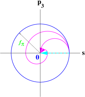
Figure 11: Schematic view of the possible paths of symmetry restoration in the chiral space. There may be possible another paths utilizing the degree of freedom of the chiral angle, besides the usual one along $\theta=0$.

4.2 DCDW in the NJL model

Taking the Nambu-Jona-Lasinio (NJL) model as a simple but nontrivial example, we explicitly demonstrate that quark matter becomes unstable for a formation of DCDW above a certain density; the NJL model has been recently used as an effective model of QCD, embodying spontaneous breaking of chiral symmetry in terms of quark degree of freedom [55] . We shall explicitly see the DCDW state exhibits a ferromagnetic property.

We start with the NJL Lagrangian with $N_{f}=2$ flavors and $N_{c}=3$ colors,

$${\cal L}_{NJL}=\bar{\psi}(i\partial/-m_{c})\psi+G[(\bar{\psi}\psi)^{2}+(\bar{\psi}i\gamma_{5}\mbox{\boldmath$\tau$}\psi)^{2}],$$ (60)

where $m_{c}$ is the current mass, $m_{c}\simeq 5$MeV. Under the Hartree approximation, we linearize Eq. (60) by partially replacing the bilinear quark fields by their expectation values with respect to the ground state.

In the usual treatment to study the restoration of chiral symmetry at finite density, authors implicitly discarded the pseudo-scalar mean-field, while this is justified only for the vacuum of a definite parity. We assume here the following mean-fields,

$$\langle\bar{\psi}\psi\rangle = \Delta\cos(\bf q\cdot\bf r)$$

$$\langle\bar{\psi}i\gamma_{5}\tau_{3}\psi\rangle = \Delta\sin(\bf q\cdot\bf r),$$ (61)

and others vanish . This configuration looks to break the translational invariance as well as rotation symmetry, but the former invariance is recovered by absorbing an additional constant by a global chiral transformation. Accordingly, we define a new quark field $\psi_{W}$ by the Weinberg transformation [60],

$$\psi_{W}=\exp[i\gamma_{5}\tau_{3}{\bf q\cdot r}/2]\psi,$$ (62)

to separate the degrees of freedom of the amplitude and phase of DCDW in the Lagrangian. In terms of the new field the effective Lagrangian renders

$${\cal L}_{MF}=\bar{\psi}_{W}[i\partial/-M-1/2\gamma_{5}\tau_{3}q/]\psi_{W}-G\Delta^{2},$$ (63)

where we put $M\equiv-2G\Delta$ and $q^{\mu}=(0,{\bf q})$, taking the chiral limit ($m_{c}=0$). The form given in (63) appears to be the same as the usual one, except the axial-vector field generated by the wave vector of DCDW; the amplitude of DCDW produces the dynamical quark mass in this case. We shall see the wave vector ${\bf q}$ is related to the magnetization: the phase of DCDW induces the magnetization. With this form we can find a spatially uniform solution for the quark wave function (see Table 3), $\psi_{W}=u_{W}(p)\exp(i{\bf p\cdot r})$, with the eigenvalues,

$$E_{p}^{\pm}=\sqrt{E_{p}^{2}+|{\bf q}|^{2}/4\pm\sqrt{({\bf p}\cdot{\bf q})^{2}+M^{2}|{\bf q}|^{2}}},~{}~{}~{}E_{p}=(M^{2}+|{\bf p}|^{2})^{1/2}$$ (64)

for positive-energy (valence) quarks with different spin polarizations (c.f. (42)).

Table 3: Diagram of the Weinberg transformation.

$\langle\bar{\psi}\psi\rangle\neq 0$	$\Longleftrightarrow$	$\langle\bar{\psi}_{W}\psi_{W}\rangle=\Delta(\neq 0)$
$\langle\bar{\psi}i\gamma_{5}\tau_{3}\psi\rangle\neq 0$		$\langle\bar{\psi}_{W}i\gamma_{5}\tau_{3}\psi_{W}\rangle=0$
		$q/2\propto\nabla\theta$   (“axial-vector”)
non-uniform		uniform

4.3 Thermodynamic potential

The thermodynamic potential is given as

$$\Omega_{\rm total} = \gamma\int\frac{d^{3}p}{(2\pi)^{3}}\sum_{s=\pm}\left[(E^{s}_{p}-\mu)\theta_{s}-E^{s}_{p}\right]+M^{2}/4G$$ (65)

$$\equiv \Omega_{\rm val}+\Omega_{\rm vac}+M^{2}/4G.$$

where $\theta_{\pm}=\theta(\mu-E^{\pm}_{p})$, $\mu$ is the chemical potential and $\gamma$ the degeneracy factor $\gamma=N_{f}N_{c}$. The first term $\Omega_{\rm val}$ is the contribution by the valence quarks filled up to the chemical potential, while the second term $\Omega_{\rm vac}$ is the vacuum contribution that is apparently divergent. We shall see both contributions are indispensable in our discussion. Once $\Omega_{\rm total}$ is properly evaluated, the equations to be solved to determine the optimal values of $\Delta$ and $q$ are

$$\frac{\delta\Omega_{\rm total}}{\delta\Delta}=\frac{\delta\Omega_{\rm total}}{\delta q}=0.$$ (66)

Since NJL model is not renormalizable, we need some regularization procedure to get a meaningful finite value for the vacuum contribution $\Omega_{\rm vac}$, which can be recast in the form,

$$\Omega_{\rm vac}=i\gamma\int\frac{d^{4}p}{(2\pi)^{4}}{\rm trln}S_{W},$$ (67)

with use of the propagator $S_{W}=(p/-M-1/2\tau_{3}\gamma_{5}q/)^{-1}$. There are various kinds of regularization and we must carefully choose the relevant one to the theoretical framework. Since the energy spectrum is no more rotation symmetric, we cannot apply the usual energy or momentum cut-off regularization (MCOR) scheme to regularize $\Omega_{\rm{vac}}$. Moreover, the regularization should be, at least, independent of the order parameters $\Delta$ and $q$. Note that this demand is essential to discuss the phase transition: improper regularizations spoil the consistency of the framework and give unphysical results for the order parameters $\Delta$ and $q$ through Eq. (66). We adopt here the proper-time regularization (PTR) scheme [61], which is one of regularizations compatible with Eq. (66) . Introducing the proper-time variable $\tau$, we eventually find

$$\Omega_{\rm vac}=\frac{\gamma}{8\pi^{3/2}}\int_{0}^{\infty}\frac{d\tau}{\tau^{5/2}}\int^{\infty}_{-\infty}\frac{dp_{z}}{2\pi}\left[e^{-(\sqrt{p_{z}^{2}+M^{2}}+q/2)^{2}\tau}+e^{-(\sqrt{p_{z}^{2}+M^{2}}-q/2)^{2}\tau}\right]-\Omega_{\rm ref},$$ (68)

which is reduced to the standard formula [55] in the limit $q\rightarrow 0$.

The integral with respect to the proper time $\tau$ is still divergent due to the $\tau\sim 0$ contribution. Regularization proceeds by replacing the lower bound of the integration range by $1/\Lambda^{2}$, which corresponds to the momentum cut-off in the MCOR scheme.

Now we examine a possible instability of quark matter with respect to formation of DCDW. In the following we first inquire the sign change of the curvature of $\Omega_{\rm total}$ at the origin (stiffness parameter), $\beta$. Expanding $\Omega_{\rm vac}$ with respect to $q$ up to $O(q^{2})$, we find

$$\Omega_{\rm vac}=\Omega_{\rm vac}^{0}+\beta_{\rm vac}q^{2}+O(q^{4})$$ (69)

where the vacuum stiffness parameter $\beta_{\rm vac}$ is given by

$$\beta_{\rm vac}=\frac{\gamma\Lambda^{2}}{16\pi^{2}}J(M^{2}/\Lambda^{2})$$ (70)

with a universal function, $J(x)=-x{\rm Ei}(-x).$ The nontrivial term originates from a vacuum polarization effect in the presence of DCDW and provides a kinetic term ($\propto(\nabla\theta)^{2}$) for DCDW . The vacuum stiffness parameter $\beta_{\rm vac}$ can be also written as $\beta_{vac}=\frac{1}{2}f_{\pi}^{2}$ [55] with the pion decay constant $f_{\pi}$, and is always positive; it gives a ’repulsive’ contribution, so that the vacuum is stable against formation of DCDW. Note that it gives a null contribution in case of $M=0$ , irrespective of $q$, as it should be.

For given $\mu,M$ and $q$ we can evaluate the contribution by the Fermi seas $\Omega_{\rm val}$ using Eq. (64), but its general formula is very complicated [53]. However, it may be sufficient to consider the small $q$ case for our present purpose. Then the thermodynamic potential can be expressed as

$$\Omega_{\rm val} = \Omega_{\rm val}^{0}-\frac{\gamma}{8\pi^{2}}M^{2}q^{2}H(\mu/M)+O(q^{4})$$ (71)

$$\equiv \Omega_{\rm val}^{0}+\Omega_{\rm val}^{mag}+O(q^{4})$$

up to $O(q^{2})$, where $H(x)={\rm ln}(x+\sqrt{x^{2}-1})$ and $\Omega_{\rm val}^{0}=\epsilon_{\rm val}^{0}-\mu\rho_{\rm val}^{0}$ with $\rho^{0}_{\rm val}=\frac{\gamma}{3\pi^{2}}(\mu^{2}-M^{2})^{3/2}$ for normal quark matter. The valence stiffness parameter then reads

$$\beta_{val}=-\frac{\gamma}{8\pi^{2}}M^{2}H(\mu/M)$$ (72)

Since the function $H(x)$ is always positive and accordingly $\beta_{val}\leq 0$, the magnetic term $\Omega_{\rm val}^{mag}$ always gives a negative energy and approaches to zero as $M\rightarrow 0$ (triviality).

We may easily understand why the valence quarks always favor the formation of DCDW. First, consider the energy spectra for massless quarks (see Fig. 12).

Figure 12: Energy spectra for ${\bf p}_{\perp}=0$. $E^{\pm}$ with $M=0$ (thick solid and dashed lines). $\tilde{E}^{\pm}$ with the definite chirality is also shown for comparison (dotted line). We can see there is a degeneracy of $E^{\pm}$ at $p_{z}=0$ for $M=0$, while it is resolved by the mass (thin solid and dashed lines).

As is already discussed, our theory becomes trivial in this case and we find two spectra

$$E^{\pm}_{p}=\sqrt{p_{\perp}^{2}+(|p_{z}|\pm q/2)^{2}},~{}~{}~{}{\bf p}_{\perp}=(p_{x},p_{y},0),$$ (73)

which are essentially equivalent to $E^{\pm}_{p}=|{\bf p}|$ with definite chirality.

There is a level crossing at ${\bf p}={\bf 0}$. Once the mass term is taken into account this degeneracy is resolved and the energy splitting arises there. Hence it causes an energy gain, if $q=O(2\mu)$; we can see that this mechanism is very similar to that of SDW by Overhauser [16, 20].

Using Eqs. (65), (69), (71) we write the thermodynamic potential as

$$\Omega_{\rm total}=\Omega_{NJL}+\beta q^{2}+O(q^{4})$$ (74)

with the total stiffness parameter $\beta=\beta_{vac}+\beta_{val}$ and the usual NJL expression without DCDW, $\Omega_{NJL}=\Omega_{\rm vac}^{0}(M)+\Omega_{\rm val}^{0}(M)+M^{2}/4G.$ The dynamical quark mass $M$ is given by the equation, $\partial\Omega_{\rm total}/\partial M=0$; At the order of $q^{0}$ the dynamical quark mass $M^{0}$ is determined by the equation, $\left.\partial\Omega_{NJL}/\partial M\right|_{M^{0}}=0.$ Since $M-M^{0}=O(q^{2})$, DCDW onsets at a certain density where the total stiffness parameter $\beta$ becomes negative: the critical chemical potential $\mu^{cr}$ is determined by the equation,

$$\beta=\frac{1}{2}f_{\pi}^{2}-\frac{\gamma}{8\pi^{2}}\left(M^{0}\right)^{2}H(\mu^{cr}/M^{0})=0.$$ (75)

Note that this is only a sufficient condition for formation of DCDW, and we can never exclude the possibility of the first-order phase transition or metamagnetism [11, 22]. Actually, we shall see that DCDW occurs as a first-order phase transition.

4.4 First-order phase transition

The values of the order parameters $M$ and $q$ are obtained from the minimum of the thermodynamic potential  (65) for $T=0$. Fig. 13 shows the contours of $\Omega_{\rm total}$ in the $M$-$q$ plane as the chemical potential increases, where the parameters are chosen as $G\Lambda^{2}=6$ and $\Lambda=850$ MeV, to reproduce the constituent quark mass in the vacuum ($\mu=0$) [55].

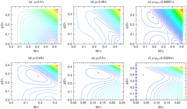
Figure 13: Contours of $\Omega_{\rm total}$ at $T=0$ are shown in $M-q$ plane as the chemical potential increases, (a) $\rightarrow$ (f). The cross in each figure denotes the absolute minimum.

The crossed points denote the absolute minima. There are two critical chemical potential $\mu=\mu_{c1},\mu_{c2}$: for the lower densities (Fig. 13(a)-(b)) the absolute minimum resides at the point $(M\neq 0,q=0)$ indicating the SSB phase. At $\mu=\mu_{c1}$ (Fig. 13(c)) the potential has the two absolute minima at $(M\neq 0,q=0)$ and $(M\neq 0,q\neq 0)$, showing the first-order transition to the DCDW phase which is stable for $\mu_{c1}<\mu<\mu_{c2}$ (Fig. (13)d-e). At $\mu=\mu_{c2}$ (Fig. 13(f)) the axis of $M=0$ and a point $(M\neq 0,q\neq 0)$ become minima, the system undergoes the first-order transition again to the chiral-symmetric phase.

Fig. 15 summarizes the behaviors of the order-parameters $M$ and $q$ as functions of $\mu$ at $T=0$, where that of $M$ without DCDW is also shown for comparison. It is found that DCDW develops at finite range of $\mu$ ($\mu_{c1}\leq\mu\leq\mu_{c2}$), where the wave number $q$ increases with $\mu$ but its value is smaller than twice of the Fermi momentum $2k_{F}$($\simeq 2\mu$ for free quarks) since the nesting of Fermi surfaces is incomplete in the present 3-D system; actually, the ratio becomes $q/k_{F}=1.17-1.47$ for the baryon-number densities $\rho_{b}/\rho_{0}=3.62-5.30$ where DCDW is stable (see Fig. 15).

Figure 14: Wave number $q$ and the dynamical mass $M$ are plotted as functions of the chemical potential at $T=0$. Solid (dotted) line for $M$ with (without) the density wave, and dashed line for $q$.

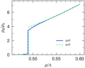
Figure 15: Baryon number density as a function of $\mu$. $\rho_{0}=0.16{\rm fm}^{-3}$: the normal nuclear density.

4.5 Correlation functions

In this section, we consider scalar- and pseudoscalar-correlation functions, $\Pi_{\rm s,sp}(k)$, in the massless limit $M\rightarrow 0$, and discuss their relation with the mechanism for DCDW. In the static limit $k_{0}\rightarrow 0$, the correlation functions have a physical correspondence to the static susceptibility for the spin- or charge-density wave [17]. We shall see that these functions have a differential singularity at $k=2k_{F}$, reflecting the sharp Fermi surface at $T=0$.

We explicitly evaluate the effective interactions, $\Gamma_{\rm s,sp}(k)$, in the pseudo-scalar and scalar channels within the random phase approximation [44, 55], which are related to the correlation functions $\Pi_{\rm s,sp}(k)$, i.e., $2G\Pi_{\rm s,sp}(k)=\Gamma_{\rm s,sp}(k)\Pi_{\rm s,sp}^{0}(k)$:

$$i\Gamma_{\rm s,ps}(k) = \frac{2Gi}{1-2G\Pi_{\rm s,ps}^{0}(k)},$$ (76)

where $\Pi_{\rm s,ps}^{0}(k)$ are the polarization functions in medium,

$$\!\!\!\!\!\!\!\!\!\!\Pi_{\rm s}^{0}(|{\bf k}|)\!\!\!\! = \!\!\!\!\Pi_{\rm ps}^{0}(|{\bf k}|)$$ (77)

$$= \!\!\!\!\!\frac{N_{f}N_{c}}{4\pi^{2}}(\Lambda^{2}-2k_{F}^{2})-2N_{f}N_{c}i{\bf k}^{2}I({\bf k}^{2})|_{M\rightarrow 0}$$

$$+ \!\!\!\!\!\frac{N_{f}N_{c}|{\bf k}|}{4\pi^{2}}\left[\!\left(k_{F}\!-\!\frac{|{\bf k}|}{2}\right)\log\left(\frac{2k_{F}\!+\!|{\bf k}|}{2k_{F}\!-\!|{\bf k}|}\right)\!+\!\frac{|{\bf k}|}{2}\log\left(\frac{2k_{F}}{|{\bf k}|}\!+\!\frac{|{\bf k}|}{2k_{F}}\right)\!\right]\!\!,\!\!$$

in the static and chiral limit [53]. It is well known that poles of the effective interaction give the energies of scalar and pseudo-scalar mesons [44, 55]. Note that the inverse of the effective interaction in the massless limit also gives the coefficient of $M^{2}$ in the effective potential in the presence of DCDW,

$$\Omega_{\rm total}=\Omega_{\rm total}|_{M\rightarrow 0}+\frac{1}{2}\Gamma_{\rm ps}^{-1}(q)|_{M\rightarrow 0}M^{2}+O(M^{4}).$$ (78)

Hence, the critical density and the critical wave vector $q_{\rm crit}$ should be given by the equations,

$$\Gamma_{\rm ps}^{-1}(q_{\rm crit})|_{M\rightarrow 0}=0,\partial\Gamma_{\rm ps}^{-1}(q)|_{M\rightarrow 0}/\partial q|_{q_{\rm crit}}=0,$$ (79)

in the case of the second-order or weakly first-order phase transition.

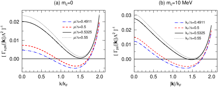
Figure 16: Function, $1/\Gamma_{\rm ps}(|{\bf k}|)$, is plotted for various Fermi momenta, $k_{F}/\Lambda=0.4752,0.5$, and $0.6$. The thick (thin) lines correspond to the chiral limit $m_{c}=0$ ($m_{c}=5$MeV). In the case of $k_{F}/\Lambda\geq 0.4752$, the mass-gap equation has a extremum solution $M=0$ in the absence of DCDW.

Fig.16 show the function $1/\Gamma_{\rm ps}(|{\bf k}|)|_{M=0}$ and we can see these conditions are almost satisfied at the terminal density, $\mu=\mu_{c2}$, due to a tiny jump in the dynamical mass (weakly first-order phase transition) . A numerical calculation in the chiral limit gives $\mu_{t}(=k_{F})=0.5320\Lambda$ and $|{\bf k}_{t}|=1.498k_{F}$, which almost coincide with the previous results given in Figs. 13 and 15, $\mu_{c2}=0.53254\Lambda$ and $q=1.469k_{F}$ (where $k_{F}\equiv\sqrt{\mu_{c2}^{2}-M^{2}}$; $M=0.034\Lambda$). On the other hand, the phase transition is of first order at the onset density, $\mu=\mu_{c1}$: there is a discontinuous jump in the dynamical mass (the amplitude of DCDW) $M$, so that the above argument cannot be applied any more. Besides, the correlation functions or the effective interactions provide a powerful tool to analyze the DCDW phase as far as the dynamically generated mass (the amplitude of DCDW) $M$ is small, as in the present case. From the behavior of the function $\Gamma_{\rm ps}(|{\bf k}|)^{-1}$ shown in Fig. 16, it is found that $\Gamma_{\rm ps}(|{\bf k}|)^{-1}$ takes the lowest value at $|{\bf k}|\sim 1.3-1.5k_{F}(O(2k_{F}))$, reflecting the sharp Fermi surface, and thus a finite wave number $q$ gives the lower potential energy in Eq. (78) than $q=0$ in the density range of DCDW. These values are consistent with those in Fig. 15, and we can see again that DCDW is closely related to the sharpness of the Fermi surface.

It should be noted again that the negative value of the function $\Gamma_{\rm ps}(|{\bf k}|)^{-1}|$ gives a necessary condition for formation of DCDW, but the sign change does not necessarily imply the critical condition in the case of first-order phase transitions, as in the present case; the terminal transition is weakly first-order and we can apply there. It should be also noted that its minimum point always gives an optimal value of the wave vector in the presence of DCDW. Thus we can see by the use of the correlation functions that the particle-hole pairing with finite momentum $q=O(2k_{F})$ effectively lowers the free energy in comparison with the zero total momentum.

The above argument might also be available even for the case of a finite current-quark mass, $m_{c}\simeq 5$MeV: Fig. 16 shows that the minimum of $\Gamma_{\rm ps}(|{\bf k}|)^{-1}$ has little shift from that in the chiral limit.

4.6 Magnetic properties

The mean-value of the spin operator is given by

$$\bar{s}_{z}=\frac{1}{2}u^{\dagger}_{W}\Sigma_{z}u_{W}=\frac{1}{2}\frac{q/2\pm\beta_{p}}{E^{\pm}_{p}}+{\rm vac},$$ (80)

with $\beta_{p}=\sqrt{p_{z}^{2}+m^{2}}$, where ”vac” means the vacuum contribution. First note that the integral of $\bar{s}_{z}$ over the Fermi seas should be proportional to $q$, and the solution with $q\neq 0$ seems to imply FM. However, we can show that PTR gives the vacuum (the Dirac sea) contribution oppositely to cancel the total mean-value of the spin operator, which is consistent with Eq. (66). Instead we can see that the magnetization spatially oscillates,

$$M_{z}\equiv\langle\bar{q}\sigma_{12}q\rangle=\langle\gamma_{0}\sigma_{12}\rangle\cos({\bf q}\cdot{\bf r}),$$ (81)

with

$$\langle\gamma_{0}\sigma_{12}\rangle=\int_{F^{+}-F^{-}}\frac{d^{3}p}{(2\pi)^{3}}\frac{2M}{\sqrt{M^{2}+p_{z}^{2}}},$$ (82)

which means a kind of spin density wave [21].

4.7 Phase diagram in the $T-\mu$ plane

To establish the phase diagram in the $T-\mu$ plane, we derive the thermodynamic potential at finite temperature in the Matsubara formalism. The partition function for the mean-field Hamiltonian is given by

$$Z_{\beta}\!\! = \!\!\!\int{\it D}\bar{\psi}{\it D}\psi\exp\int_{0}^{\beta}\!\!\!d\tau\!\!\!\int d^{3}r~{}\!\!\left\{\bar{\psi}\left[i\tilde{\partial}+M\exp\left(i\gamma_{5}{\bf q}\cdot{\bf r}\right)\!-\!\gamma_{0}\mu\right]\psi\!-\!\frac{M^{2}}{4G}\right\}$$ (83)

$$= \prod_{{\bf k},n,s=\pm}\left\{(i\omega_{n}+\mu)^{2}-E_{s}^{2}({\bf k})\right\}^{N_{f}N_{c}}\times\exp\left\{-\left(\frac{M^{2}}{4G}\right)V\beta\right\},$$

where $\beta=1/T$, $\tilde{\partial}\equiv-\gamma_{0}\partial_{\tau}+i{\bf\gamma}\nabla$ and $\omega_{n}$ the Matsubara frequency. Thus the thermodynamic potential $\Omega_{\beta}$ is obtained,

$$\Omega_{\beta}(q,M)\!\!\! = \!\!\!-T\log{Z_{\beta}(q,M)}/V$$ (84)

$$= \!\!\!-N_{f}N_{c}\!\!\int\!\!\frac{d^{3}{\rm k}}{(2\pi)^{3}}\!\!\sum_{s}\!\!\left\{T\log{\left[e^{-\beta\left(E_{s}({\bf k})-\mu\right)}\!\!+\!\!1\right]\left[e^{-\beta\left(E_{s}({\bf k})+\mu\right)}\!\!+\!\!1\right]}\!\!+\!\!E_{s}({\bf k})\right\}$$

$$+\frac{M^{2}}{4G}.$$

From the absolute minima of the thermodynamic potential (84), it is found that the order parameters at $T\neq 0$ behave similarly to those at $T=0$ as a function of $\mu$, while the chemical-potential range of the DCDW at finite temperature, $\mu_{c1}(T)\leq\mu\leq\mu_{c2}(T)$, gets smaller as $T$ increases. We show the resultant phase diagram in Fig. 17, where the ordinary chiral-transition line is also given. Comparing phase diagrams with and without $q$, we find that the DCDW phase emerges in the area (closed area in Fig. 17) which lies just outside the boundary of the ordinary chiral transition. We thus conclude that the DCDW is induced by finite-density contributions, and has an effect to expand the chiral-condensed phase ($M\neq 0$) toward low temperature and high density region.

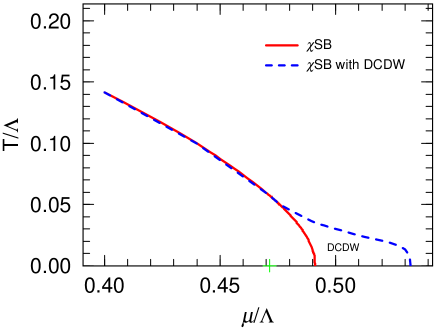
Figure 17: Phase diagram obtained from the thermodynamic potential  (84). The solid (dashed) line shows the chiral-restoration boundary in the presence (absence) of DCDW. The closed area denoted by “DCDW” shows the DCDW phase.

5 Summary and Concluding remarks

We have seen some magnetic aspects of quark matter: ferromagnetism at high densities and spin density wave at moderate densities within the zero-range approximation for the interaction vertex. These look to follow the similar development about itinerant electrons: Bloch mechanism at low densities and spin density wave at high densities by Overhauser.

By a perturbative calculation with the OGE interaction, we have seen ferromagnetism in quark matter at low densities (§2.1) . It would be worth mentioning that another study with higher-order diagrams qualitatively supports it [34]. These studies suggest an opposite tendency to the one using the zero-range interaction (§§2.2,2.3). Note that we can also see the same situation for itinerant electrons; the Hartree-Fock calculation based on the infinite-range Coulomb interaction favors ferromagnetism at a low density region, while the Stoner model, which introduces the zero-range effective interaction instead of the Coulomb interaction, gives ferromagnetism at high densities. So we must carefully examine the possibility of ferromagnetism in quark matter by taking into account the finite-range effect.

We have examined the coexistence of spin polarization and color superconductivity by choosing a quark pair with the same polarization. We have introduced the axial-vector self-energy and the quark pair field (the gap function), whose forms are derived from the one-gluon-exchange interaction by way of the Fierz transformation under the zero-range approximation. Within the relativistic Hartree-Fock framework we have evaluated their magnitudes in a self-consistent manner by way of the coupled Schwinger-Dyson equations.

As a result of numerical calculations spontaneous spin polarization occurs at a high density for a finite quark mass in the absence of CSC, while it never appears for massless quarks as an analytical result. In the spin-polarized phase the single-particle energies corresponding to spin degrees of freedom, which are degenerate in the non-interacting system, are split by the exchange energy in the axial-vector channel. Each Fermi sea of the single-particle energy deforms in a different way, which causes an asymmetry in the two Fermi seas and then induces the axial-vector mean-field in a self-consistent manner. In the superconducting phase, however, spin polarization is slightly reduced by the pairing effect; it is caused by competition between reduction of the deformation and enhancement of the difference in the phase spaces of opposite “spin” states due to the anisotropic diffuseness in the momentum distribution.

We have also noted another possibility of the pairing: the quark pair with opposite polarization to each other. It may lead to a gapless superconductor, but we need a further study.

We have seen that dual chiral desnity wave (DCDW) appears at a certain density and develops at moderate densities (§3). It occurs as a result of the interplay between the $\bar{q}q$ and particle-hole correlations. The phase transition is of weakly first order, and the restoration of chiral symmetry is delayed compared with the usual scenario.

For the discussion of DCDW given in §4, we have seen the remarkable roles of the Fermi sea and the Dirac sea: the former always favors DCDW, while the latter works against it. The similar situation also appears about the magnetic property of quark matter. The mean value of the spin operator over the Fermi seas of valance quarks always gives a finite value in the presence of DCDW, which is a kind of ferromagnetism, but the vacuum contribution given by the Dirac seas completely cancels it. As a result there is no net spin polarization in this case, but we have seen magnetization spatially oscillates instead (spin density wave). This is one of the typical examples in which the nonrelativistic picture is qualitatively different from the relativistic one by the vacuum effect.

It would be interesting to recall that DCDW is similar to pion condensation within the $\sigma$ model, considered by Dautry and Nyman [56], where $\sigma$ and $\pi^{0}$ meson condensates take the same form as Eq. (61). So it might be intriguing to connect pion condensation before deconfinement with DCDW after it in light of symmetry consideration. Note that this type of hadron-quark continuity has been also suggested in the context of hadron and quark superconductivities [62].

If ferromagnetism is realized in quark matter, it may give a microscopic origin of the magnetic field in compact stars; actually we have seen that it can give a possible explanation for the superstrong magnetic field observed in magnetars, if they are quarks stars. It would be challenging to explain other characteristic phenomena in magnetars such as a sudden braking down observed in a soft gamma-ray repeater SGR 1806-20 or SGR 1900+14 [63]; some global reconfiguration of of the magnetic has been suggested for these phenomena [64]. It would be also ambitious to give a scenario based on magnetic properties of quark matter, which can explain the hierarchy of the magnetic field observed in three classes of neutron stars, magnetars, radio pulsars and recycled millisecond pulsars. Ferromagnetism may give a permanent magnetization and there is no field decay, in difference from the dynamo mechanism caused by the charged current.

The magnetic phases considered here accompany the symmetry breaking, $SO(3)\rightarrow O(2)$, so that we can expect the Nambu-Goldstone modes as lowest excitations in the ground state: spin wave in ferromagnetism and phason in DCDW. It should be interesting to study these modes. Such low excitation modes may affect the thermal evolution of compact stars [65]. It would be also interesting to investigate how the effective interaction by exchanging such excitations between quarks affects superconductivity.

References

-
[1]
M. Alford, Ann. Rev. Nucl. Part.Sci., 51 (2001)
131.
D.H. Rischke, Prog. Part. Nucl. Phys. 52 (2004) 197. -
[2]
For recent reviews of lattice simulations, F. Karsh,
Lect. Notes Phys. 583 (2002) 209.
E. Laermann and O. Philipsen, hep-ph/0303042. -
[3]
F. Weber, Pulsars as Astrophysical Laboratories for
Nuclear and Particle Physics (IOP Publishing Ltd., Bristol,
1999).
N. Glendenning, Compact Stars (Springer, New York, 1996). -
[4]
D. Bailin and A. Love, Phys. Reports 107(1984) 325.
As a review, K. Rajagopal and F. Wilczek, hep-ph/0011333. - [5] M. Tinkham, Introduction to Superconductivity (McGraw-Hill, New York, 1975).
- [6] For a review, G. Chanmugam, Annu. Rev. Astron. Astrophys. 30 (1992) 143.
- [7] P.M. Woods and C.J. Thompson, astro-ph/0406133.
-
[8]
A.I. Ibrahim et al., Astrophys. J. 574 (2002) L51
N. Rea et al., Astrophys. J. 586 (2003) L65.
G.F. Bignami et al., astro-ph/0306189. - [9] K. Makishima, Prog. Theor. Phys. Suppl. 151 (2003) 54.
- [10] For recent results, S. Fantoni et al., Phys. Rev. Lett. 87 (2001) 181101; I. Vidana and I. Bombaci, Phys. Rev. C66 (2002) 045801.
- [11] T. Tatsumi, Phys. Lett. B489 (2000) 280.
- [12] M. Alford, K. Rajagopal and F. Wilczek, Nucl. Phys. B537 (1999) 443; J. Berges and K. Rajagopal, Nucl. Phys. B538 (1999) 215; T. M. Schwarz, S. P. Klevansky and G. Papp, Phys. Rev. C60 (1999) 055205; D.Ebert, V.V.Khudyakov, V.Ch.Zhukovsky and K.G.Klimenko, Phys. Rev. D65 (2002) 054024.
- [13] L.N. Buaevskii et al., Adv. Phys. 34 (1985) 175.
- [14] S.S. Sexena et al., Nature 406 (2000) 587; C.Pfleiderer et al., Nature 412 (2001) 58; N.I.Karchev et al., Phys. Rev. Lett. 86 (2001) 846.
- [15] D.V. Deryagin, D. Yu. Grigoriev and V.A. Rubakov, Int. J. Mod. Phys. A7 (1992) 659.
-
[16]
B.-Y. Park, M.Rho, A.Wirzba and I.Zahed, Phys. Rev. D62 (2000) 034015.
R. Rapp, E.Shuryak and I. Zahed, Ohys. Rev. D63 (2001) 034008. - [17] S. Kagoshima, H. Nagasawa, and T. Sambongi, One Dimensional Conductors, Springer series in solid-state sciences, Vol. 72 (Springer-Verlag, Berlin, 1988); L. P. Gor’kov and G. Grüner, Charge Density waves in Solids, MODERN PROBLEMS IN CONDENSED MATTER SCIENCES. VOL. 25 (AMSTERDAM: North-Holland, 1989).
- [18] R. E. Peierls, Quantum Theory of Solids (Oxford University Press, London, 1955).
- [19] G. Grüner, Rev. Mod. Phys. 60 (1988) 4.
- [20] A.W. Overhauser, Phys. Rev. 128 (1962) 1437.
- [21] G. Grüner, Rev. Mod. Phys. 66 (1994) 1.
- [22] F. Bloch, Z. Phys. 57 (1929) 545;
-
[23]
C. Herring, Exchange Interactions among Itinerant
Electrons: Magnetism IV (Academic press, New
York, 1966)
K. Yoshida, Theory of magnetism (Springer, Berlin, 1998). - [24] K.A. Brueckner and K. Sawada, Phys. Rev. 112 (1957) 328.
- [25] D.M. Ceperley and B.J. Alder, Phys. Rev. Lett. 45 (1980) 566.
- [26] D.P. Young et al., Nature 397 (1999) 412.
- [27] e.g.,C. Itzykson and J.-B. Zuber, Quantum Field Theory (McGraw-Hill Inc., 1980).
-
[28]
V.B. Berestetsii, E.M. Lifshitz and L.P. Pitaevsii,
Relativistic Quantum Theory (Pergamon Press, 1971). - [29] G. Baym and S.A. Chin, Nucl. Phys. A262 (1976) 527.
- [30] I.A. Akhiezer and S.V. Peletminskii, JETP 11 (1960) 1316.
- [31] e.g.,R. Tamagaki and T. Tatsumi, Prog. Theor. Phys. Suppl. 112 (1993) 277.
- [32] T. DeGrand et al., Phys. Rev. D12 (1975)2060.
- [33] E. Farhi and R.L. Jaffe, Phys. Rev. D30 (1984) 2379.
- [34] A. Niegawa, hep-ph/0404252.
- [35] For a review, J. Madsen, astro-ph/9809032.
- [36] J.I.Kapusta, Finite-Temperature field theory (Cambridge Univ. Press, 1989); M. LeBellac, Thermal Field Theory (Cambridge Univ. Press, Cambridge, Eingland, 1996)
- [37] E. Nakano, K. Nawa and T. Tatsumi, in preparation.
- [38] E. Nakano, T. Maruyama and T. Tatsumi, Phys. Rev. D68 (2003) 105001; T. Tatsumi, T. Maruyama and E. Nakano, Prog. Theor. Phys. Suppl. 153 (2004) 190; hep-ph/0312351.
-
[39]
T. Schafer, Phys. Rev. D62 (2000) 094007.
M. Buballa, J. Hosek and M. Oertel, Phys. Rev. Lett. 90 (2003) 182002.
A. Schmitt, Q. Wang and D.H. Rischke, Phys. Rev. D66 (2002) 114010; Phys. Rev. Lett. 91 (2003) 242301;Phys. Rev. D69 (2004) 094017. - [40] A. J. Leggett, Rev. Mod. Phys. 47 (1975) 331.
- [41] R. Tamagaki, Prog. Theor. Phys. 44 (1970) 905; M. Hoffberg, A.E. Glassgold, R.W. Richardson and M. Ruderman, Phys. Rev. Lett. 24 (1970) 775.
- [42] M. Alford, J.A. Bowers, J.M. Cheyne and G.A. Cowan, hep-ph/0210106.
- [43] G.Ripka, Quarks Bound by Chiral Fields (Oxford Univ. Press, 1997).
- [44] Y. Nambu and G. Jona-Lasinio, Phys. Rev. (1961) 345.
-
[45]
P. Fulde and R.A. Ferrell, Phys. Rev. 135 (1964)
550.
A.I. Larkin and Y. Ovchinikov, Sov. Phys.-JETP 20 (1965) 762. - [46] For a review article, R. Casalbuoni and G. Nardulli, Rev. Mod. Phys. 76 (2004) 263.
-
[47]
M. Alford, J. Berges and K. Rajagopal,
Phys. Rev. Lett. 84 (2000) 598.
W.V. Liu and F. Wilczeck, Phys. Rev. Lett. 90 (2003) 047002.
I. Shovkovy and H. Huang, Phys. Lett. B564 (2003) 205.
E. Gubankova, W.V. Liu and F. Wilczek, hep-ph/0304016.
M.G. Alford, J. Kouvaris and K. Rajagopal, hep-ph/0311286. - [48] For a recent review, M. Huang, hep-ph/0409167.
-
[49]
P.F. Bedaque, H. Caldas and R. Rupak,
Phys. Rev. Lett. 91 (2003) 247002.
H. Caldas, hep-ph/0312275. -
[50]
I. Shovkovy, M. Hanauske and M. Huang, Phys. Rev. D67 (2003) 103004.
S. Reddy and R. Rupak, nucl-th/0405054. - [51] K. Nawa, E. Nakano and T. Tatsumi, in progress.
- [52] N. Karchev, Phys. Rev. B67(2003) 054416.
- [53] T. Tatsumi and E. Nakano, hep-ph/0408294; E. Nakano and T. Tatsumi, hep-ph/0411350.
-
[54]
T. Eguchi and H. Sugawara, Phys. Rev. D10 (1974) 4257.
K. Kikkawa, Prog. Theor. Phys. 56 (1974) 947. -
[55]
S.P. Klevansky, Rev. Mod. Phys. 64 (1992) 649.
T. Hatsuda and T. Kunihiro, Phys. Rep. 247 (1994) 221. -
[56]
F. Dautry and E.M. Nyman, Nucl. Phys. 319 (1979) 323.
- [57] M. Kutschera, W. Broniowski and A. Kotlorz, Nucl. Phys. A516 (1990) 566.
- [58] K. Takahashi and T. Tatsumi, Phys. Rev. C63 (2000) 015205; Prog. Theor. Phys. 105 (2001) 437.
-
[59]
M. Sadzikowski and W. Broniowski, Phys. Lett. 488 (2000) 63.
M. Sadzikowski, Phys. Lett. 553 (2003) 45. - [60] S. Weinberg, The quantum theory of field II(Cambridge, 1996).
- [61] J. Schwinger, Phys. Rev. 92 (1951) 664.
- [62] T. Schaefer and F. Wilczek, Phys. Rev. Lett. 82 (1999) 3956.
- [63] C. Kouveliotou et al., Nature 393 (1998) 235; Ap.J 510 (1999) L115.
- [64] P.M. Woods et al., astro-ph/0101045.
-
[65]
S. Tsuruta, Phys. Reports 292 (1998) 1.
D.G. Yakovlev and C.J. Pethick, astro-ph/002143.