Chromoelectric fields and quarkonium-hadron interactions at high energies

Abstract

We develop a simple model to study the heavy quarkonium-hadron cross section in the high energy limit. The hadron is represented by an external electric color field (capacitor) and the heavy quarkonium is represented by a small color dipole. Using high energy approximations we compute the relevant cross sections, which are then compared with results obtained with other methods.

I Introduction

Quarkonium-hadron cross sections ($\sigma_{\Phi h}$) are a necessary tool to understand the forthcoming data on quarkonium production, which will become available at RHIC. In the last six years many efforts have been devoted to this problem nos1 and real progress has been achieved, especially in what concerns the cross sections at low energies, close to the dissociation threshold. In the energy region far from threshold the situation is less clear and even the energy dependence is still subject of debate. Extrapolation from calculations valid at low energies points to different directions. Results obtained with the non-relativistic quark model wongs indicate a rapidly falling cross section. This behavior is due to the gaussian tail of the quark wave functions used in the quark exchange model. This same behavior could be found within chiral meson Lagrangian approaches with the introduction of $\sqrt{s}$ dependent form factors osl . In QCD sum rules regras the cross section was found to be monotonically increasing with energy.

The calculations of $\sigma_{\Phi h}$ designed to be valid at high energies ($\sqrt{s}\simeq 20$ GeV) are quite few: the Bhanot-Peskin (BP) approach pes ; kar ; kar2 ; arleo ; oh ; song , perturbative QCD plus geometrical extrapolation gerland , the model of the stochastic vacuum (MSV) dnnr and the light-cone dipole formalism huf2000 . During the last years the leading order BP approach has been used very often. However, the recent next to leading order calculations presented in song show that, for the charmonium, the formalism breaks down because this system is not heavy enough. Most of the calculations mentioned above predict a rising cross section. In Ref. oh , $\sigma_{\Phi h}$ falls with the energy and in Ref. dnnr it stays constant.

If the quarkonium is treated as an ordinary hadron, its cross section for interaction with any other ordinary hadron must increase smoothly at higher energies, in much the same way as the proton-proton or pion-proton cross sections. The underlying reason is the increasing role played by perturbative QCD dynamics and the manifestation of the partonic nature of all hadrons. However this partonic picture starts to be dominant only at much higher energies ($\sqrt{s}\,\rangle\,100$ GeV). In the energy region relevant for RHIC physics non-perturbative aspects are still very important. In the high energy calculations mentioned above, different non-perturbative ingredients were employed: moments of the gluon distribution in the hadron pes ; kar ; kar2 ; arleo ; oh ; song ; hadron and quarkonium wave functions gerland and QCD vacuum expectation values (condensates) dnnr .

Since there are still discrepancies concerning numbers (which may vary by one order of magnitude for different estimates) and the energy behavior, we think that it is interesting to calculate $\sigma_{\Phi h}$ with a non-perturbative approach, putting emphasis on the role played by the chromoelectric fields. In benzahra a similar treatment was adopted to study the quarkonium dissociation inside a QCD plasma. The color electric fields appearing in the transition matrix element were related to the color charge density of the medium, which, in turn, was computed in a specific model of the QGP. Here we start with a similar expression for the transition amplitude but, since we are in a purely hadronic phase, we must know the chromoelectric field inside nucleons and pions. There has been progress in the study of these fields, coming from models of the QCD vacuum michael , from lattice QCD suga , from the Field Correlator Method (FCM) simonov and from Coulomb gauge QCD adam . We hope that we can benefit from these advances and use the profiles of the chromoelectric fields estimated in these works in our problem. For this purpose, we treat the interaction between the quarkonium and hadron as being analogous to the interaction of a small dipole traversing a large capacitor and interacting with the color electric field but not with its sources. In the final part of this work we discuss the validity of this last assumption. Using a contact interaction between a heavy quark (or antiquark) and a quark (or antiquark) we compute the corresponding cross section and find that it is indeed much smaller than the heavy quark-external field cross section. The model developed here bears some resemblance to the Bhanot-Peskin picture, but is much simpler. Some simplifying assumptions are used to render the calculations quasi analytic and preserve the understanding of the basic physics.

II The model

II.1 The interaction Hamiltonian

The starting point is the assumption that the quarkonium (dipole) is small compared with the hadron (capacitor). As a consequence, the $\overline{Q}-Q$ pair will interact mostly with the external color field but not with the (quark) sources. Moreover, the external color field is considered to have only low momentum components (“soft gluons”) and thus is able to transfer only a small amount of energy, which will be barely enough to dissociate the bound state. In the case of the charmonium, the typical binding energy is $\epsilon\simeq 0.6$ GeV. Therefore, in a first approximation

$$\epsilon\ll M_{\Phi}$$ (1)

where $M_{\Phi}$ is the mass of the bound state ($M_{\Phi}\simeq 3$ GeV). In the case of the bottonium this approximation is even better. The binding energy is also small compared to the collision energy

$$\epsilon\ll\sqrt{s}$$ (2)

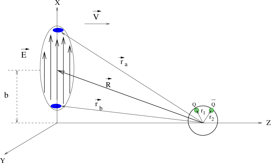
Figure 1: Quarkonium-hadron interaction in the quarkonium rest frame. The hadron is a capacitor moving to the right. The $\vec{E}^{a}$ field is along the $x$ direction. The thick black dots are the capacitor ”plates”: quark-antiquark for the pion and quark-diquark for the proton.

Inequality (1) justifies the use of quantum mechanical perturbation theory (the Born approximation) and inequality (2) justifies the use of the eikonal approximation, which, in this case, implies that the hadron follows a straight line trajectory and remains essentially undisturbed during the interaction. In Figure 1 we present our picture of the scattering and our choice of coordinates, in the quarkonium rest frame: $\vec{r}_{1}$ and $\vec{r}_{2}$ are the quark and antiquark coordinates and $\vec{E}^{a}$ is the chromoelectric field in the projectile, which will be a proton or a pion, moving with constant velocity $\vec{v}$ at impact parameter $\vec{b}$.

With these assumptions we can write the interaction Hamiltonian as:

$$H_{int}=g(T^{a}_{1}\vec{E}^{a}_{1}\vec{r}_{1}+\overline{T}^{b}_{2}\vec{E}^{b}_{2}\vec{r}_{2})$$ (3)

where $T^{a}$ ($\overline{T}^{b}$) are the generators of color group SU(3) in the fundamental (conjugate) representation. $\vec{E}^{a}_{1}$ and $\vec{E}^{b}_{2}$ are the chromoelectric fields generated by the hadron in motion (capacitor) and “felt” by quark and antiquark in the bound state respectively. They have to be Lorentz transformed to the quarkonium rest frame, bringing to our calculation a Lorentz gamma factor, which is the source of the energy dependence ($\sqrt{s}$) of our results. We shall for the moment neglect the magnetic component, since it does not do any work on the charges and thus is not effective in the energy transfer. Besides, the magnetic interaction is inversely proportional to the quark mass, being thus suppressed.

We can represent this external field by:

$$\vec{E}^{a}(r_{e},t) = \gamma\vec{E}^{a}_{0}\,\,exp\left(-\frac{(X-x_{e})^{2}}{d^{2}}-\frac{(Y-y_{e})^{2}}{d^{2}}\right)\,\,exp\left(-\gamma^{2}\frac{\left[vt-z_{e}\right]^{2}}{d^{2}}\right)$$ (4)

with $e=1,2$ . X, Y and Z are the hadron coordinates and $\gamma$ is the usual Lorentz factor. $Z=vt$, because the hadron moves with velocity $\vec{v}$ along the z axis. $\vec{E}^{a}_{0}$, which will be abreviated by $E$, is the color electric field at the center of the projectile. The projectile mean square radius is related to the parameter $d$ through:

$$\sqrt{\langle r^{2}_{h}\rangle}\,=\,0.86\,\,d$$

We neglect the deflection of the hadron trajectory, because we are studying reactions in the high energy and non-perturbative regime, i.e., with low momentum transfer. X and Y are related with the impact parameter $b$ by: $b^{2}=X^{2}+Y^{2}$. Notice that, by simplicity, we choose one preferencial direction for the field, in this case, the $x$-axis.

Neglecting the CM motion, (3) can be rewritten as

$$H_{int}=g(\frac{\lambda^{a}}{2}E^{a}_{1}+\frac{\lambda^{{b}^{T}}}{2}E^{b}_{2})(\frac{x_{1}-x_{2}}{2})$$ (5)

Also for the sake of simplicity, when working with (5), we will take $x_{1}-x_{2}\simeq a$, where $a$ is the typical separation between quark and antiquark. Initially the quark-antiquark pair is in a localized region of the space.

II.2 The initial state

The initial wave function of system has spatial and color parts defined by:

$$\Psi_{i}=f(r_{1},r_{2})c_{n}d_{n}$$ (6)

where $c_{n}$ and $d_{n}$, with $n=1,2,3$, are the initial color vectors griff for quark and antiquark respectively, taken in a color singlet state. We choose

$$f(r_{1},r_{2})=N_{i}\,exp[{-\frac{\vec{r}_{1}\,^{2}}{{a}^{2}}}]\,exp[{-\frac{\vec{r}_{2}\,^{2}}{{a}^{2}}}]\,exp(-i\varepsilon_{i}t)$$ (7)

where $\varepsilon_{i}$ ($\varepsilon_{i}=M_{\Phi}$) is the quarkonium initial energy and $N_{i}$ is a normalization constant given by:

$$N^{2}_{i}=(\frac{2}{\pi})^{3}\,\frac{1}{a^{6}}$$

The initial wave function $\Psi_{i}$ describes the confinement of quarks and also asymptotic freedom, as it allows the quarks to be independent inside the bag. It is easy to see that the connection between the quarkonium mean square radius and the parameter $a$ is

$$\sqrt{\langle r^{2}_{Q\overline{Q}}\rangle}\,=\,1.09\,\,a$$

II.3 The final state

Under the action of the external field the initial wave function $\Psi_{i}$ evolves to a final state $\Psi_{f}$:

$$\Psi_{f}=t(r_{1},r_{2})c_{j}d_{k}$$ (8)

where $c_{j}$ and $d_{k}$, with $j,k=1,2,3$, are the quark and antiquark final color vectors and $t(r_{1},r_{2})$ the spatial part of the wave function. In the final state of this reaction we have to deal with the transition of a pair of an excited quark and an antiquark to a pair of mesons $D$ - $\overline{D}$ (or $B-\overline{B}$). This transition is highly non-perturbative and has to be modelled. We shall use here two approaches.

model A

We first assume that the quark and antiquark are converted into two free mesons (a $M$ and a $\overline{M}$) which are thus described by plane waves:

$$t_{A}(r_{1},r_{2}) = N_{A}\,\,exp\,(i\vec{p}_{1}.\vec{r}_{1})\,\,exp\,(i\vec{p}_{2}.\vec{r}_{2})\,\,exp\,(-i\varepsilon_{f}t)$$ (9)

where $\vec{p}_{1}$ and $\vec{p}_{2}$ are the meson momenta and $N_{A}$ is a normalization constant given by:

$$N^{2}_{A}=\frac{1}{V^{2}}$$

with $V$ being an arbitrary normalization volume, which will be cancelled in the calculation of the cross section. In the above expression $\varepsilon_{f}$ is the final energy of the $Q-\overline{Q}$ pair. The energy transferred during the reaction must be sufficient to dissociate the bound state into a pair of mesons with open charm ($D\overline{D}$) or beauty ($B\overline{B}$) and therefore:

$$\varepsilon_{f}=\sqrt{(\vec{p}_{1})^{2}+m_{M}^{2}}\,\,+\,\,\sqrt{(\vec{p}_{2})^{2}+m_{\overline{M}}^{2}}$$ (10)

where $m_{M}$ ($m_{\overline{M}}$) is the mass of the meson coming out from the fragmentation of the quark (antiquark). With this definition of $\varepsilon_{f}$ we implicitly account for the conversion of quarks into hadrons, a process which cannot be better described in this simple model.

The assumptions (9) and (10) are reasonable but they represent a case of ”extreme freedom” : they do not take into account the energy loss from a parent quark when it is converted to a (less energetic) final meson. This process is described, in certain situations, by the fragmentation functions. Morevover, the final mesons can have any momentum and even though higher momenta will be naturally suppressed in the calculation, we are overestimating the phase space of the reaction.

model B

Given these weak points of (9) and (10) we shall also use a second approach for the final state which is more conservative. We shall assume that the energy transferred to the heavy quarkonium $\Phi$ will transform it into an excited (but still bound) state $\Phi^{\prime}$. The mass of this excited state will be taken to be slightly higher than the first charmonium and bottonium excitations $\Psi^{\prime}$ and $\Upsilon^{\prime}$ respectively. It is known that these excitations are very weakly bound. Therefore, by choosing slightly higher masses for them, which are above the $D$-$\overline{D}$ and $B$-$\overline{B}$ decay thresholds, we are simulating a fragmentation process to a pair of nearly at rest mesons. This assumption is complementary to (9) and (10) since here we give to the heavy quarks only the ”minimal freedom”. The ground state wave function was chosen to be the Gaussian (7). Taking the harmonic oscillator as inspiration, we choose the wave function of the first excited state as a function which is odd in the $x$ direction (this is the direction of the chromoelectric field) and symmetric in $x_{1}$ and $x_{2}$:

$$t_{B}(r_{1},r_{2}) = N_{B}\,\frac{x_{1}+x_{2}}{2}\,exp[{-\frac{\vec{r}_{1}\,^{2}}{{a^{\prime}}^{2}}}]\,exp[{-\frac{\vec{r}_{2}\,^{2}}{{a^{\prime}}^{2}}}]\,exp(-i\varepsilon_{f}t)$$ (11)

where the normalization constant is:

$$N^{2}_{B}=(\frac{4}{\pi})^{3}\,\frac{1}{{a^{\prime}}^{8}}$$

and $a^{\prime}$ is related to the size of the state $\Psi^{\prime}$ or $\Upsilon^{\prime}$. Using the wave function (11) has some advantages. In first place, it avoids the definition of a fragmentation mechanism with the introduction of new parameters. In second place, as it can be seen, (11) is orthogonal to (9), so that the matrix element $<\Psi_{f}|H_{int}|\Psi_{i}>$ is zero if the Hamiltonian is a constant. Notice that this does not happen when we use (9) and therefore the approach A might contain spurious contributions. The same comment is valid for the calculations made in Ref. benzahra . This makes the contrast between approaches A and B even more necessary. Finally, in what follows we shall use the Hamiltonian (3), without the approximation $x_{1}-x_{2}\simeq a$ made in model A.

Transition amplitudes and cross sections

The transition amplitude for model A can be easily computed from (5), (4), (6), (8) and (9):

$$T_{fi}=\langle\Psi_{f}|H_{int}|\Psi_{i}\rangle=\int dt\int d^{3}\vec{r}_{1}\int d^{3}\vec{r}_{2}\,\,\Psi^{*}_{f}(\vec{r}_{1},\vec{r}_{2})H_{int}(\vec{r}_{1},\vec{r}_{2})\Psi_{i}(\vec{r}_{1},\vec{r}_{2})$$ (12)

An analogous expression holds for model B with the use of (3), (4), (6), (8) and (11). We next take the amplitude squared $|T_{fi}|^{2}=T_{fi}^{*}\,T_{fi}$ and since color is not observed, we take the average of the all initial color states and the sum of all final states:

$$|T_{fi}|^{2}\to\overline{|T_{fi}|^{2}}\equiv\frac{1}{3}\sum_{n}\frac{1}{8}\sum_{a}\sum_{j}\sum_{k}|T_{fi}|^{2}$$ (13)

The cross section with model A is given by:

$$\sigma_{A}=\int\frac{V}{(2\pi^{3})}d^{3}p_{1}\,\int\frac{V}{(2\pi^{3})}d^{3}p_{2}\,2\pi\int_{0}^{\infty}db\,b\,\overline{|T_{fi}|^{2}}$$ (14)

The above expression is very simple and can be calculated almost analytically. Because of the gaussian Ansatz (4) and (6) we can easily integrate (12) over the coordinates and over the impact parameter. In the last step of (14), the integration over the phase space had to be done numerically. In fkn we made the additional assumption that the outgoing mesons are nearly at rest and we could thus simplify (10) and perform the integration over $\vec{p}_{1}$ and $\vec{p}_{2}$ analytically. Here we prefer to be more “exact” and perform the last integrations numerically.

The cross section with model B is simply given by:

$$\sigma_{B}=2\pi\int_{0}^{\infty}db\,b\,\overline{|T_{fi}|^{2}}$$ (15)

which, after the proper substitutions and integrations yields:

$$\sigma_{B}=\frac{32}{3}\pi^{5}\,\,\langle gE_{0}\rangle^{2}\,\,\frac{\gamma^{2}}{\gamma^{2}-1}\,\,\frac{d^{10}\,a^{\prime 8}\,a^{10}}{(a^{\prime 2}+a^{2})^{5}[a^{\prime 2}a^{2}+d^{2}(a^{\prime 2}+a^{2})]^{3}}\,\,exp{\Big{(}-\omega^{2}\frac{\frac{\gamma^{2}a^{\prime 2}a^{2}}{(a^{\prime 2}+a^{2})}+d^{2}}{2(\gamma^{2}-1)}\Big{)}}$$ (16)

where:

$$\omega=\varepsilon_{f}-\varepsilon_{i}\,\,=\,\,M_{\Phi^{\prime}}-M_{\Phi}$$ (17)

From the above expression we can observe that the cross section rises with the energy ($\gamma$) and saturates at a constant value. The enhancement of the chromoelectric field is tamed by the Lorentz contraction of the projectile. As for the size parameters, $a$, $a^{\prime}$ and $d$, the cross section first rises and then falls with increasing values of the parameters. The values of the maxima strongly depend on the model and might change for a different choice of wave functions. However, the physical picture is very simple. Expression (16) tells us that the probability of converting a quarkonium of given initial size $a$ to a final state with size $a^{\prime}$ tends to zero if $a^{\prime}=0$ or if $a^{\prime}\to\infty$ because the overlap between these very different states and the initial state is zero. For the same reason the cross section vanishes for $a=0$ and for $a\to\infty$. The parameter $d$ is associated with the extension of the capacitor. When it goes to infinity the spatial dependence of the potential disappears, it becomes a constant and then $<\Psi_{f}|H_{int}|\Psi_{i}>\to<\Psi_{f}|\Psi_{i}>=0$.

II.4 The interaction with the sources

In the introduction it was assumed that the quarkonium is well represented by a small dipole, which traverses a large capacitor. However this may be a too strong assumption because the dipole is not always so small. For example, comparing the size of the charmonium with the size of pion we have tipically $\frac{a}{d}\simeq\frac{0.4}{0.6}\simeq 0.67$. Therefore it is necessay to include the interaction between the quark and antiquark in the quarkonium with the sources (the ”plates” of the capacitor) which may be either a quark and an antiquark in the case of the pion or quark and a diquark in the case of the proton.

In order to take these interactions into account we shall assume that the interaction between a quark (or diquark) in the capacitor and a charm quark (or antiquark) in the dipole can be divided into a short distance and a long distance part. The later was already included before in the interaction with the chromoelectric fields produced by the sources. The former will be modelled as follows.

model C

The short distance interaction can be approximated by the contact interaction part (the one with the delta function) of the one-gluon exchange potential brac :

$$H_{int}=V_{OGE}=\sum_{i=a,b}\sum_{j=1,2}\frac{\alpha_{s}}{4}\vec{\lambda_{i}}\cdot\vec{\lambda_{j}}\Big{(}\frac{1}{r_{ij}}\,-\,\frac{2\pi}{3m_{i}m_{j}}\vec{\sigma_{i}}\cdot\vec{\sigma_{j}}\delta^{3}(\vec{r_{ij}})\Big{)}$$ (18)

where $\lambda$ and $\sigma$ are the Gell-Mann and Pauli matrices respectively, which are responsible for color and spin interactions. The Coulomb term in the above expression will be neglected because it is of long range. The labels $i=a,b$ and $j=1,2$ refer to particles in the capacitor and dipole respectively. With this notation, in the interaction between particle $a$ and $1$ the delta function above takes the form:

$$\delta^{3}(\vec{r_{a}}-\vec{r_{1}})=\delta(x_{a}-x_{1})\times\delta(y_{a}-y_{1})\times\delta(z_{a}-z_{1})$$ (19)

where $\vec{r_{1}}=(x_{1},y_{1},z_{1})$ is the same as before and $\vec{r_{a}}=(x_{a},y_{a},z_{a})$ is the coordinate of the particle $a$ in the quarkonium rest frame. In order to compute the transition amplitude we need to know the new wave functions, which now include both the quarkonium and the capacitor. They are:

$$\Psi_{i}=f(\vec{r_{1}},\vec{r_{2}})g(\vec{r_{a}},\vec{r_{b}})c_{n}d_{n}e_{m}h_{m}$$ (20)

and

$$\Psi_{f}=t_{C}(\vec{r_{1}},\vec{r_{2}})g(\vec{r_{a}},\vec{r_{b}})c_{i}d_{j}e_{l}h_{k}$$ (21)

In the above expression the function $f$ is the same as before and given by (7). The function $t_{C}$ represents the spatial distribution of the heavy quarks in the final state, which is assumed to be an excited but still bound state, very much like in model B. However, if we would choose $t_{C}=t_{B}$, the transition amplitude $<\Psi_{f}|H_{int}|\Psi_{i}>$ would vanish because the contact interaction does not depend on the coordinates and hence $<\Psi_{f}|\Psi_{i}>$ is the product of an odd by an even function of $x$, being thus zero. Since we are mostly interested in knowing the order of magnitude of this contact interaction we shall approximate the final state wave function by a gaussian, given by:

$$t_{C}(\vec{r_{1}},\vec{r_{2}})=N_{C}\,exp{(\frac{-r^{2}_{1}}{a^{{}^{\prime}2}})}\,exp{(\frac{-r^{2}_{2}}{a^{{}^{\prime}2}})}\,e^{-i\varepsilon_{f}t}\,$$ (22)

with the normalization constant given by:

$$N_{C}^{2}=\Big{(}\frac{2}{\pi}\Big{)}^{3}\frac{1}{a^{\prime 6}}$$ (23)

The computation of the contact interaction requires the knowledge of the positions of the quarks in the capacitor, which is given by the function $g$

$$g(\vec{r_{b}},\vec{r_{b}}) = N_{P}\,exp{\Big{[}\frac{-(x_{a}-X)^{2}}{d^{2}}\Big{]}}exp{\Big{[}\frac{-(y_{a}-Y)^{2}}{d^{2}}\Big{]}}$$ (24)

$$\times exp{\Big{[}\frac{-(x_{b}-X)^{2}}{d^{2}}\Big{]}}exp{\Big{[}\frac{-(y_{b}-Y)^{2}}{d^{2}}\Big{]}}$$

$$\times exp{\Big{[}\frac{-\gamma^{2}(z_{a}-Z)^{2}}{d^{2}}\Big{]}}exp{\Big{[}\frac{-\gamma^{2}(z_{b}-Z)^{2}}{d^{2}}\Big{]}}$$

where $Z=vt$, $d$ and $\gamma$ have the same meaning as before and $N_{P}$ is the normalization constant of the projectile wave function, given by:

$$N_{P}^{2}=\frac{8\gamma^{2}}{\pi^{3}d^{6}}$$ (25)

Notice that $g$ is the same in the initial and in the final state. This assumption is consistent with the eikonal approximation introduced above and avoids the introduction of new parameters.

With these ingredients we can evaluate the transition amplitude:

$$T_{fi} = \langle\Psi_{f}|H_{int}|\Psi_{i}\rangle$$ (26)

$$= \int dt\int d^{3}\vec{r}_{1}d^{3}\vec{r}_{2}\int d^{3}\vec{r_{a}}d^{3}\vec{r_{b}}\,\,\Psi^{*}_{f}(\vec{r}_{1},\vec{r}_{2},\vec{r_{a}},\vec{r_{b}})\,H_{int}(\vec{r}_{1},\vec{r}_{2},\vec{r_{a}},\vec{r_{b}})\,\Psi_{i}(\vec{r}_{1},\vec{r}_{2},\vec{r_{a}},\vec{r_{b}})$$

and the cross section:

$$\sigma_{C} = \frac{2^{10}}{3^{4}}\pi\alpha_{s}^{2}\,\,\Big{(}\frac{1}{m_{a}m_{1}}+\frac{1}{m_{a}m_{2}}+\frac{1}{m_{b}m_{1}}+\frac{1}{m_{b}m_{2}}\Big{)}^{2}$$ (27)

$$\times \,\frac{\gamma^{2}}{\gamma^{2}-1}\,\,\frac{a^{6}a^{\prime 6}}{(a^{\prime 2}+a^{2})^{5}[d^{2}(a^{\prime 2}+a^{2})+2a^{2}a^{\prime 2}]}\,\,exp{\Big{(}-\omega^{2}\frac{\frac{\gamma^{2}a^{\prime 2}a^{2}}{(a^{\prime 2}+a^{2})}+d^{2}}{4(\gamma^{2}-1)}\Big{)}}$$

where we have used (13) and the analogous expression for the sum and average over spins. Apart from a numerical factor, (16) and (27) have the same energy dependence. This is so because the same Lorentz contraction in the exponent of the Hamiltonian (3) and (4) leading to (16) is now present in the capacitor wave function (24). Moreover, the same Lorentz $\gamma$ factor, previously multiplying the $\vec{E}^{a}$ field in (4) reappears now in the normalization constant (25). The dependence of (27) on $a$ and $a^{\prime}$ is qualitatively the same as the one found in (16) and has the same physical origin. Finally, the cross section above is now a monotonically decreasing function of $d$. The observed behavior with $d$ means that, in a larger capacitor the quarks are spread across a larger transverse area and it becomes more difficult for them to find the charm quarks in the target and suffer a contact interaction.

III Results and discussion

In the numerical estimates presented below, we shall adopt $d=0.8$ and $0.6$ fm for the proton and the pion respectively. We shall also take $a=0.4$ and $0.2$ fm for the $J/\psi$ and $\Upsilon$ respectively and $a^{\prime}=0.8$ and $0.45$ fm for the $\Psi^{\prime}$ and $\Upsilon^{\prime}$. The bound states $\Psi$ ($m_{\Psi}=3.07$ GeV) and $\Upsilon$ ($m_{\Upsilon}=9.46$ GeV) will be, in model A, dissociated into pairs of mesons $D$ ($m_{D}=1.87$ GeV) and $B$ ($m_{B}=5.27$ GeV). The excited states used in models B and C have masses $m_{\Phi^{\prime}}=3.8$ GeV and $m_{\Phi^{\prime}}=11$ GeV in the case of charmonium and bottonium respectively. The value of the strong coupling constant and the constituent quark masses are the same used in brac , i.e., $\alpha_{s}=0.64$, $m_{q}=0.3$ GeV, $m_{c}=1.2$ GeV, $m_{b}=4.74$ GeV and the diquark mass is $m_{d}=0.60$ GeV.

As it is clear from (5) and (4), we need to know the average value of the color electric field in the projectile $gE\,=\,\langle h|gE|h\rangle$. In a first approximation this number might be identified with the string tension $\kappa\simeq 0.18$ $GeV^{2}$ or $\kappa\simeq 0.9$ $GeV/fm$. The string tension calculated in adam is somewhat larger. In simonov the transverse profile of the string was studied. The strength of $\langle h|gE|h\rangle$ depends on the quark-antiquark (or quark-diquark) separation, being larger for larger systems and so far it has been calculated only for large systems. Therefore $\langle h|gE|h\rangle$ is another source of differences between a proton and a pion projectile. Taking an average of the values found in simonov we choose $\langle h|gE|h\rangle=1$ GeV/fm.

As mentioned in the introduction, our model has common aspects with the BP approach. Therefore we shall, in what follows, compare our results for $\sigma_{\Phi h}$ with those obtained by Kharzeev in kar2 :

$$\sigma_{\Phi h}=2.5\,\,\left(1\,\,-\,\,\frac{\lambda_{0}}{\lambda}\right)^{6.5}\,\,\mbox{mb}$$ (28)

with $\lambda$ given by

$$\lambda\simeq\frac{(s-M^{2}_{\Phi})}{2M_{\Phi}}$$ (29)

and $\lambda_{0}\simeq(M_{h}+\varepsilon)$, where $M_{h}$ is the projectile mass and

$$\varepsilon=2\,m_{M}-M_{\Phi}.$$ (30)

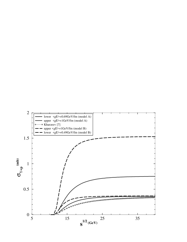
Figure 3: Same as Fig. 2 for the $\Upsilon+p$ cross section.

In Figure 2 we show the cross sections for the proton-charmonium dissociation obtained with model A (dotted lines) and model B (dashed lines) and compare them with the BP cross section (solid line with stars) given by (28). The two upper curves are obtained with $\langle h|gE|h\rangle=1$ GeV/fm and the two lower curves with $\langle h|gE|h\rangle=0.57$ GeV/fm (model A) and $\langle h|gE|h\rangle=0.53$ GeV/fm (model B). With these smaller values of the chromoelectric field our curves come close to (28). Figure 3 shows the corresponding cross sections for the proton-bottonium dissociation. Again, the two upper curves are obtained with $\langle h|gE|h\rangle=1$ GeV/fm and the two lower curves with $\langle h|gE|h\rangle=0.69$ GeV/fm (model A) and $\langle h|gE|h\rangle=0.49$ GeV/fm (model B). As in the previous figure, reducing the value of $\langle h|gE|h\rangle$ leads to some agreement with (28). Given the conceptual resemblance between our model and the BP one, it is reassuring to find a certain similarity between the results, both in magnitude and energy behavior, once an appropriate value of $\langle h|gE|h\rangle$ is chosen.

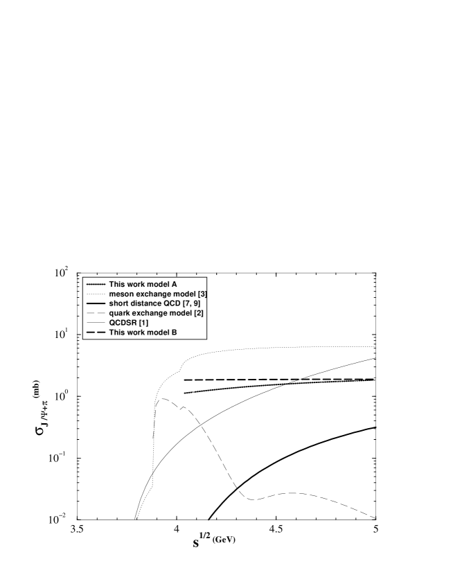
Figure 4: Pion-charmonium cross section as a function of $\sqrt{s}$ with several models.

In Figure 4 we show the cross section for $J/\psi$ dissociation by pions compared with results obtained the meson exchange model osl (thin dotted line), with the quark exchange model wongs (thin long dashed line), with short distance QCD (the BP approach) Eq. (28) (thick solid line) and QCD sum rules nos1 (thin solid line). In spite of the fact that, at such low energies our approach looses validity, it is, nevertheless, interesting to observe that our curve is in the center of the region covered by the other calculations. In Figure 5 we compare the cross sections $p\,-\,J/\psi$ (upper curves) and $\pi\,-\,J/\psi$ (lower curves) calculated with models A (dotted lines) and B (dashed lines). In the high energy limit, where both cross sections are nearly constant, we observe that the relation between the cross sections is:

$$\sigma_{p-\Phi}\,\simeq\,3\,\sigma_{\pi-\Phi}\,\,\,\,\,\,\mbox{model A}$$ (31)

$$\sigma_{p-\Phi}\,\simeq\,4.2\,\sigma_{\pi-\Phi}\,\,\,\,\,\,\mbox{model B}$$ (32)

which in both cases is much larger than the one expected from the additive quark model:

$$\sigma_{p-\Phi}\,\simeq\frac{3}{2}\,\sigma_{\pi-\Phi}$$ (33)

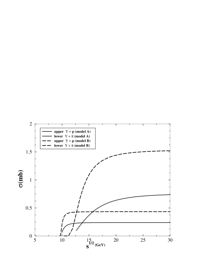
Figure 6: Same as Fig. 5 for bottonium-hadron cross sections.

This is remarkable since the additive quark model relation holds for other high energy scattering processes like $\pi-p$ and $p-p$. Since $\langle h|gE|h\rangle$ was kept the same for both cases, this unexpected relation between the cross sections must come from differences in the wave functions. In Figure 6 we repeat this comparison for the reactions $p\,-\,\Upsilon$ and $\pi\,-\,\Upsilon$, finding (31) for both models. We have kept $\langle h|gE|h\rangle=1$ GeV/fm for both projectiles. Taking $\langle p|gE|p\rangle>\langle\pi|gE|\pi\rangle$ would increase the deviation from (33).

In the high energy limit ordinary hadrons are expected to have a geometrical total cross section. Since the quarkonium dissociation discussed here is a more specific reaction it is not obvious that its cross section follows a geometrical behavior. Such a behavior was found in arleo : $\sigma_{\Phi h}\propto\alpha_{s}a_{0}^{2}$ where $a_{0}$ is the Bohr radius of the quarkonium. In our case, as it can be seen from (16), (27) and from the numerical evaluation of (14), we have a very non-trivial dependence on $a$. Since the initial state (containing the variable $a$) is the same, the difference between models comes from the spatial dependence of the final state. The plane waves in model A have no spatial scale. Therefore they are more ”inclusive” and so $\sigma_{A}$ should be closer to the quarkonium-hadron total cross section than $\sigma_{B}$. In model B the quarkonium ground state is converted into a resonance-like state, which wave function contains the size parameter of the resonance and distorts the final geometrical behavior. Therefore model A is closer to a geometrical behavior than model B.

In order to see how far we are from the geometrical behavior, we show in Figures 7 and 8 the dependence of $\sigma_{A}$ (dotted line) and $\sigma_{B}$ (dashed line) on $a$ for charmonium (Fig. 7) and bottonium (Fig. 8) dissociation. The cross sections are divided by $a^{2}$ so that geometrical behavior translates into a horizontal line. We see that, whereas model A tends to this behavior, model B is far from a geometrical behavior. This indicates again that our model is very sensitive to the choice of the final state wave functions.

In Figure 9 we show the cross section $\sigma_{C}$ (27) for charmonium dissociation by protons (solid line) and by pions (dashed line). In Figure 10 we show the same quantitity for bottonium dissociation. We use the central values for $a$, $a^{\prime}$, $d$ and $\alpha_{s}$. We can see that, in all processes, the cross sections are more than two orders of magnitude smaller than the corresponding cross sections computed with model A or model B. No possible change in parameters could make these cross sections comparable. Another feature of these curves is that the cross sections for $J/\psi$ dissociation by pions are larger than those for protons by a factor close to $4$. This might be guessed looking at (27). The pion is light quark-antiquark system and the proton is light quark-diquark dipole. The diquark is twice heavier than a constituent quark. Whereas for the pion $m_{b}=m_{a}$, for the proton we have $m_{b}=2m_{a}$.

Before concluding we would like to make a remark concerning medium effects on the cross sections calculated above. We are primarily studying reactions which happen before thermalization (in nucleus-nucleus collisions) or with no thermalization at all (in proton-nucleus collisions). The formation time of the heavy quark pair is of the order of $0.2$ fm. The thermalization time of hadronic matter formed in heavy ion collisions is a model dependent quantity. Early estimates pointed to $1$ fm. Recent estimates heinz point to $0.6$ fm. Even taking seriously this last number, it is fair to say that heavy quark pair production (and collision with a hadron at high energies) precedes the formation of an equilibrated medium. After thermalization, the energy is completely redistributed and collisions occur at energies of the order of the temperature ($<1$ GeV). In this regime we do not expect our approach to be valid. The effects of a thermal medium on the heavy quarkonium are known wong : the string tension becomes weaker, the quarkonium size increases and its mass decreases. These effects are, all of them, very small except if we get close to the deconfinement transition temperature. In view of these considerations we have neglected medium effects in our calculations.

IV Conclusions

We have developed a simple model for the non-perturbative quarkonium-hadron interaction. At the present stage of the field, this sort of model is still useful to organize the ideas. We tried to make simple and yet realistic choices for the interaction Hamiltonian and for the wave functions. In particular we have treated the final state in two very different and complementary ways. Simple models are not appropriate to provide very precise results but they can help in determining the order of magnitude of the cross sections and their behavior with the reaction energy. Having said that, we can summarize our conclusions as follows.
i) The charmonium-hadron cross section is of a few milibarns. The bottonium-hadron cross section is about four times smaller. This is in agreement with most of the previous calculations.
ii) All cross sections grow with the reaction energy and reach a plateau in the high energy limit. This is in agreement with the BP approach.
iii) In this limit they do not obey the simple relations derived from the additive quark model.
iv) Also in this limit our cross sections deviate significantly from the geometrical behavior ($\sigma\propto a^{2}$).
v) The contact interactions between the heavy quarks and the light quarks in the light hadrons is negligible compared to the long-distance quark - $\vec{E}^{a}$ field interaction. This is surprising since sometimes the dipole and the capacitor have similar sizes. This finding gives a posteriori support to our model and also to the BP approach.

Conclusion i) may be relevant for RHIC and LHC physics. Conclusions ii, iii and iv suggest that the heavy quarkonium has interaction properties which are very different from light hadrons. This has been conjectured before. In particular, in dnw this difference was attributed to the fact that in heavy quarkonia the energy is mainly stored in the masses whereas in light hadrons the energy (mass of the hadron) comes mostly from the gluonic fields.

Acknowledgements: This work has been supported by CNPq and FAPESP. We are indebted to M. Nielsen, D.A. Fogaça and F. Durães for fruitful discussions.

Figure 2: $J/\psi-p$ cross section with model A (dotted lines), model B (dashed lines) and with the Bhanot-Peskin approach (lines with stars). Upper curves: stronger $\vec{E}^{a}$ field. Lower curves: weaker $\vec{E}^{a}$ field.

Figure 5: Charmonium-hadron cros section with model A (dotted lines) and model B (dashed lines). Upper curves: $\sigma_{J/\psi}-p$. Lower curves $\sigma_{J/\psi}-\pi$.

Figure 7: Charmonium-hadron cross sections as a function of the charmonium size parameter for model A (dotted line) and for model B (dashed line).

Figure 8: Same as Fig. 7 for bottonium-hadron cross sections.

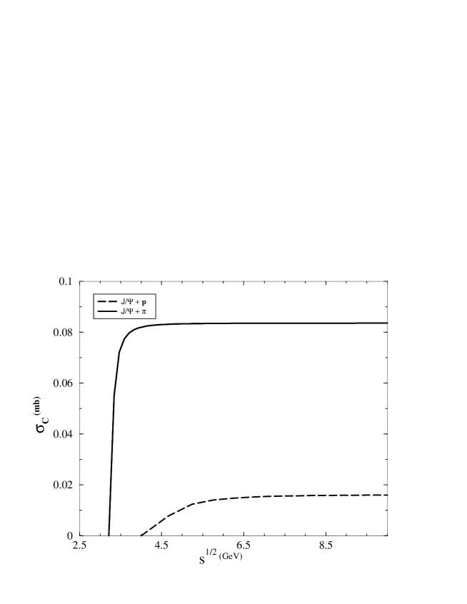
Figure 9: Charmonium-proton (dashed line) and charmonium-pion (solid line) cross sections calculated with model C (contact interactions).

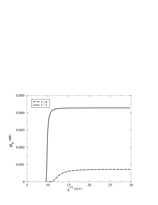
Figure 10: Same as Fig. 9 for bottonium-hadron cross sections.

References

- (1) For a recent review, see F.O. Durães et al., Phys. Rev. C68, 035208 (2003).
- (2) C.-Y. Wong, E. S. Swanson and T. Barnes, Phys. Rev. C62, 045201 (2000); C65, 014903 (2001).
- (3) Y. Oh, T. Song and S.H. Lee, Phys. Rev. C63, 034901 (2001).
- (4) F.S. Navarra et al., Phys. Lett. B 529, 87 (2002); M. Nielsen et al., Braz. Jour. Phys. 33 , 316 (2003); F.O. Durães et al., Phys. Lett. B564, 97 (2003).
- (5) M.E. Peskin, Nucl. Phys. B156, 365 (1979) ; G. Bhanot and M.E. Peskin, Nucl. Phys. B156, 391 (1979).
- (6) D.Kharzeev and H. Satz, Phys. Lett. B366, 316 (1996); B356, 365 (1995); B334, 155 (1994).
- (7) D. Kharzeev, nucl-th/9601029.
- (8) F. Arleo, P.B. Gossiaux, T. Gousset and J. Aichelin, Phys. Rev. C65, 014005 (2002) .
- (9) Y. Oh, S. Kim and S.H. Lee, Phys. Rev. C65 067901 (2002).
- (10) Taesoo Song and Su Houng Lee, hep-ph/0501252.
- (11) L. Gerland et al., Phys. Rev. Lett. 81, 762 (1998).
- (12) H.G. Dosch, F.S. Navarra, M. Nielsen and M. Rueter, Phys. Lett. B466, 363 (1999).
- (13) J. Hüfner, Y.P. Ivanov, B.Z. Kopeliovich and A.V. Tarasov, Phys. Rev. D62, 094022 (2000).
- (14) B. Müller, nucl-th/9806023; S.C. Benzahra, Phys. Rev. C61, 064906 (2000).
- (15) M. Rueter and H.G. Dosch, Z. Phys. C66, 245 (1995).
- (16) T.T. Takahashi, H. Matsufuru, Y. Nemoto and H. Suganuma, Phys. Rev. Lett. 86, 18 (2001); Phys. Rev. D65, 114509 (2002); T.T. Takahashi and H. Suganuma, Phys. Rev. Lett. 90, 182001 (2003).
- (17) V.Kuzmenko and Y.A. Simonov, Phys. Lett. B494, 81 (2000); V. Kuzmenko, hep-ph/0204250.
- (18) P.O. Bowman and A.P. Szczepaniak, Phys. Rev. D70, 016002 (2004).
- (19) We are using the notation introduced in D. Griffiths, Introduction to Elementary Particles, J. Wiley and Sons, 1987, Chapter 9.
- (20) D.A. Fogaça, M.S. Kugeratski and F.S. Navarra, Braz. Jour. Phys. 34 , 276 (2004).
- (21) J. Vijande, F. Fernandez, A. Valcarce, B. Silvestre-Brac, Eur. Phys. J. A19, 383 (2004); S. Godfrey and N. Isgur, Phys. Rev. D32, 189 (1985).
- (22) F.O. Durães et al., Braz. J. Phys. 35, 3 (2005); 28, 505 (1998).
- (23) For a recent review see, U. Heinz, hep-ph/0407360.
- (24) O. Kaczmarek and F. Zantow, hep-lat/0503017 and references therein; C.-Y. Wong, hep-ph/0408020 and references therein.