Quark Loop Contributions to Neutron EDM from R-parity Violation

Abstract:

We present a detailed analysis together with numerical calculations on one-loop contributions to the neutron electric dipole moment from supersymmetry without R parity, focusing on the quark-scalar loop contributions. Complete formulas are given for the various contributions through the quark dipole operators. Analytical expressions illustrating the explicit role of the R-parity violating parameters are given following perturbative diagonalization of mass-squared matrices for the scalars. Dominant contributions come from the combinations $B_{i}^{\ast}\lambda^{\prime}_{ij1}$ for which we obtain robust bounds. Even if the R-parity violating couplings are real, CKM phase does induce RPV contribution and for some cases such a contribution is as strong as contribution from phases in the R-parity violating couplings. Hence, we have bounds directly on $|B_{i}^{\ast}\lambda^{\prime}_{ij1}|$ even if the parameters are all real.

1 Introduction

Forty years after the discovery of CP-violation[1], its experimentally observed effects in the K and B-meson systems [2] are generally compatible with the standard model (SM) predictions with the Kobayashi-Maskawa (KM) phase as its sole source. Electric dipole moments (EDMs) of elementary particles are likely to be the best candidate for the evidence of CP violating physics beyond the SM. The presence of an EDM itself violates CP[3]. Neutron being electrically neutral, is studied extensively by experimentalists, for a possible nonvanshing EDM. In the SM, the KM phase generated EDM of neutron is of the order $10^{-32}$ ecm [4], being still way below the current experimental bound of $6.3\times 10^{-26}\,\mbox{ecm}$ [5].

Many extensions of the SM are expected to give potentially large EDM contributions. For instance, in the minimal supersymmetric standard model (MSSM), which is no doubt the most popular candidate theory for physics beyond SM, the plausible extra EDM contribution of substantial magnitude has led to the SUSY-CP problem[6]. If one simply takes the minimal supersymmetric spectrum of the SM and imposes nothing more than the gauge symmetries while admitting soft SUSY breaking, the generic supersymmetric standard model (GSSM)[7] would result. When the large number of baryon or lepton number violating terms are removed by imposing an ad hoc discrete symmetry called R-parity, one obtains the MSSM Lagrangian. GSSM is a complete theory of supersymmetry (SUSY) without R-parity, where all kinds of R-parity violating (RPV) terms are admitted without bias. It is generally better motivated than ad hoc versions of RPV theories. The MSSM itself, without extension such as adding SM singlet superfields and admitting violation of lepton number, cannot accommodate neutrino mass mixings and hence oscillations [8]. Given SUSY, the GSSM is actually conceptually the simplest framework to accommodate the latter. The large number of a priori arbitrary R-parity violating terms do make phenomenology complicated. However, the origin of the (pattern of) values for the couplings may be considered to be on the same footing as that of the SM Yukawa couplings. For example, it has been shown in [9] that one can understand the origin, pattern and magnitude of all the R-parity violating terms as a result of a spontaneously broken anomalous Abelian family symmetry model.

The simplest approach to study quantum corrections to the neutron EDM is to analyze loop contributions to the $u$ and $d$ quark dipole moments and obtain the overall neutron number based on the valence quark model[10]. The neutron EDM is given by

$$d_{n}={1\over 3}\left(4\,d_{d}-d_{u}\right)\,\eta\;,$$ (1)

where $\eta\simeq 1.53$ is a QCD correction factor from renormalization group evolution[11, 12]. In the case that only trilinear RPV couplings are admitted, it has been shown that nonvanishing results come in only starting at two-loop level[13]. Striking one-loop contributions are, however, identified and discussed based on the GSSM framework[14, 15]. Similarly, flavor off-diagonal dipole moment contributing to the case of the $b\rightarrow s\gamma$ in [16] decay and that of the $\mu\rightarrow e\gamma$ [17] decay at one-loop level have also been presented. That is the approach taken here. In Ref.[14], the one loop EDM contributions from the gluino loop, chargino-like loop, neutralino-like loop are studied numerically in some details. It shows that the RPV parameter combination $\mu_{i}^{*}\lambda^{\!\prime}_{i\scriptscriptstyle 1\!1}$ dominates with small sensitivity to the value of $\tan\!\beta$. The experimental bound on neutron EDM is used to constrain the model parameter space, especially the RPV part. The deficiency of Ref.[14], missing details of quark(-scalar loop), is made up here. We give complete 1-loop formulas for the type of contributions to the EDMs of the up- and down-sector quarks, with full incorporation of family mixings. We present numerical analysis of quark-scalar loop contributions from all possible combinations of RPV parameters. Besides the familiar $\mu_{i}^{*}\lambda^{\!\prime}_{i\scriptscriptstyle 1\!1}$, there are a list of combinations of the type $B_{i}^{*}\lambda^{\!\prime}_{ijk}$ which are particularly interesting and will be the focus of this paper. Such a calculation has not been reported before. Hence, we obtain bounds on combinations of RPV couplings which are otherwise unavailable. Our study also guides plausible experimental searches for RPV SUSY signals at the next generation neutron EDM experiments.

We skip the details of the MSSM contribution to neutron EDM since it has already been extensively discussed in the literature [18].

2 Formulation and Notation

We summarize the model here while setting the notation. Details of the formulation adopted is elaborated in Ref.[7]. The most general renormalizable superpotential for the supersymmetric SM (without R-parity) can be written as

$$W\!\! = \!\varepsilon_{ab}\Big{[}\mu_{\alpha}\hat{H}_{u}^{a}\hat{L}_{\alpha}^{b}+h_{ik}^{u}\hat{Q}_{i}^{a}\hat{H}_{u}^{b}\hat{U}_{k}^{\scriptscriptstyle C}+\lambda_{\alpha jk}^{\!\prime}\hat{L}_{\alpha}^{a}\hat{Q}_{j}^{b}\hat{D}_{k}^{\scriptscriptstyle C}$$ (2)

$$+ \frac{1}{2}\,\lambda_{\alpha\beta k}\hat{L}_{\alpha}^{a}\hat{L}_{\beta}^{b}\hat{E}_{k}^{\scriptscriptstyle C}\Big{]}+\frac{1}{2}\,\lambda_{ijk}^{\!\prime\prime}\hat{U}_{i}^{\scriptscriptstyle C}\hat{D}_{j}^{\scriptscriptstyle C}\hat{D}_{k}^{\scriptscriptstyle C}\;,$$

where $(a,b)$ are $SU(2)$ indices, $(i,j,k)$ are the usual family (flavor) indices, and $(\alpha,\beta)$ are extended flavor index going from $0$ to $3$. In the limit where $\lambda_{ijk},\lambda^{\!\prime}_{ijk},\lambda^{\!\prime\prime}_{ijk}$ and $\mu_{i}$ all vanish, one recovers the expression for the R-parity preserving case, with $\hat{L}_{0}$ identified as $\hat{H}_{d}$. Without R-parity imposed, the latter is not a priori distinguishable from the $\hat{L}_{i}$’s. Note that $\lambda$ is antisymmetric in the first two indices, as required by the $SU(2)$ product rules, as shown explicitly here with $\varepsilon_{\scriptscriptstyle 12}=-\varepsilon_{\scriptscriptstyle 21}=1$. Similarly, $\lambda^{\!\prime\prime}$ is antisymmetric in the last two indices, from $SU(3)_{\scriptscriptstyle C}$.

The large number of new parameters involved, however, makes the theory difficult to analyze. An optimal parametrization, called the single-VEV parametrization (SVP) has been advocated[19] to make the the task manageable. Here, the choice of an optimal parametrization mainly concerns the 4 $\hat{L}_{\alpha}$ flavors. Under the SVP, flavor bases are chosen such that : 1) among the $\hat{L}_{\alpha}$’s, only $\hat{L}_{0}$, bears a VEV, i.e. $\langle\hat{L}_{i}\rangle\equiv 0$; 2) $h^{e}_{jk}(\equiv\lambda_{0jk})=\frac{\sqrt{2}}{v_{\scriptscriptstyle 0}}\,{\rm diag}\{m_{\scriptscriptstyle 1},m_{\scriptscriptstyle 2},m_{\scriptscriptstyle 3}\}$; 3) $h^{d}_{jk}(\equiv\lambda^{\!\prime}_{0jk}=-\lambda_{j0k})=\frac{\sqrt{2}}{v_{\scriptscriptstyle 0}}{\rm diag}\{m_{d},m_{s},m_{b}\}$; 4) $h^{u}_{ik}=\frac{\sqrt{2}}{v_{\scriptscriptstyle u}}V_{\!\mbox{\tiny CKM}}^{\!\scriptscriptstyle T}\;{\rm diag}\{m_{u},m_{c},m_{t}\}$, where ${v_{\scriptscriptstyle 0}}\equiv\sqrt{2}\,\langle\hat{L}_{0}\rangle$ and ${v_{\scriptscriptstyle u}}\equiv\sqrt{2}\,\langle\hat{H}_{u}\rangle$. The big advantage of here is that the (tree-level) mass matrices for all the fermions do not involve any of the trilinear RPV couplings, though the approach makes no assumption on any RPV coupling including even those from soft SUSY breaking; and all the parameters used are uniquely defined, with the exception of some possibly removable phases.

The soft SUSY breaking part of the Lagrangian in GSSM can be written as follows :

$$V_{\rm soft} = \epsilon_{\!\scriptscriptstyle ab}B_{\alpha}\,H_{u}^{a}\tilde{L}_{\alpha}^{b}+\epsilon_{\!\scriptscriptstyle ab}\left[\,A^{\!\scriptscriptstyle U}_{ij}\,\tilde{Q}^{a}_{i}H_{u}^{b}\tilde{U}^{\scriptscriptstyle C}_{j}+A^{\!\scriptscriptstyle D}_{ij}H_{d}^{a}\tilde{Q}^{b}_{i}\tilde{D}^{\scriptscriptstyle C}_{j}+A^{\!\scriptscriptstyle E}_{ij}H_{d}^{a}\tilde{L}^{b}_{i}\tilde{E}^{\scriptscriptstyle C}_{j}\,\right]+{\rm h.c.}$$ (3)

$$+ \epsilon_{\!\scriptscriptstyle ab}\left[\,A^{\!\scriptscriptstyle\lambda^{\prime}}_{ijk}\tilde{L}_{i}^{a}\tilde{Q}^{b}_{j}\tilde{D}^{\scriptscriptstyle C}_{k}+\frac{1}{2}\,A^{\!\scriptscriptstyle\lambda}_{ijk}\tilde{L}_{i}^{a}\tilde{L}^{b}_{j}\tilde{E}^{\scriptscriptstyle C}_{k}\right]+\frac{1}{2}\,A^{\!\scriptscriptstyle\lambda^{\prime\prime}}_{ijk}\tilde{U}^{\scriptscriptstyle C}_{i}\tilde{D}^{\scriptscriptstyle C}_{j}\tilde{D}^{\scriptscriptstyle C}_{k}+{\rm h.c.}$$

$$+ \tilde{Q}^{\dagger}\tilde{m}_{\!\scriptscriptstyle{Q}}^{2}\,\tilde{Q}+\tilde{U}^{\dagger}\tilde{m}_{\!\scriptscriptstyle{U}}^{2}\,\tilde{U}+\tilde{D}^{\dagger}\tilde{m}_{\!\scriptscriptstyle{D}}^{2}\,\tilde{D}+\tilde{L}^{\dagger}\tilde{m}_{\!\scriptscriptstyle{L}}^{2}\tilde{L}+\tilde{E}^{\dagger}\tilde{m}_{\!\scriptscriptstyle{E}}^{2}\,\tilde{E}+\tilde{m}_{\!\scriptscriptstyle H_{\!\scriptscriptstyle u}}^{2}\,|H_{u}|^{2}$$

$$+\frac{M_{\!\scriptscriptstyle 1}}{2}\tilde{B}\tilde{B}+\frac{M_{\!\scriptscriptstyle 2}}{2}\tilde{W}\tilde{W}+\frac{M_{\!\scriptscriptstyle 3}}{2}\tilde{g}\tilde{g}+{\rm h.c.}\;,$$

where we have separated the R-parity conserving ones from the RPV ones ($H_{d}\equiv\hat{L}_{0}$) for the $A$-terms. Note that $\tilde{L}^{\dagger}\tilde{m}_{\!\scriptscriptstyle\tilde{L}}^{2}\tilde{L}$, unlike the other soft mass terms, is given by a $4\times 4$ matrix. Explicitly, $\tilde{m}_{\!\scriptscriptstyle{L}_{00}}^{2}$ is $\tilde{m}_{\!\scriptscriptstyle H_{\!\scriptscriptstyle d}}^{2}$ of the MSSM case while $\tilde{m}_{\!\scriptscriptstyle{L}_{0k}}^{2}$’s give RPV mass mixings.

Details of the tree-level mass matrices for all fermions and scalars are summarized in Ref.[7]. For the analytical appreciation of many of the results, approximate expressions of all the RPV mass mixings are very useful. The expressions are available from perturbative diagonalization of the mass matrices[7].

3 The Quark Loop Contributions

We perform calculations of the one-loop EDM diagrams using mass eigenstates with their effective couplings. The approach frees our numerical results from the mass-insertion approximation more commonly adopted in the type of calculations, while analytical discussions based of the perturbative diagonalization formulae help to trace the major role of the RPV couplings, especially those of the bilinear type. The interesting class of one-loop contributions largely overlooked by other authors on RPV physics consist of a bilinear-trilinear parameter combinations. The bilinear parameters come into play through mass mixings induced among the fermions and scalars (slepton and Higgs states), while the trilinear parameter enters a effective coupling vertex. The basic features are the same as those reported in the studies of the various related processes[14, 16, 18]. Among the latter, our recently available reports on $b\rightarrow s+\gamma$ [16] are particularly noteworthy, for comparison. The $d$ quark dipole plays a more important role over that of the $u$ quark, when RPV contributions are involved. The $b\rightarrow s+\gamma$ diagram is, of course, nothing other than a flavor off-diagonal version of a down-sector quark dipole moment diagram.

The SM Yukawa couplings are real and flavor diagonal, not to say very small for the $u$ and $d$ quarks. However, the RPV analogs are mostly not so strongly constrained in magnitudes[20] and are sources of flavor mixings. A trilinear $\lambda_{\alpha jk}^{\!\prime}$ coupling couples a quark to another one, of the same or different charge, and a generic scalar, neutral or charged accordingly. The coupling together with a SM Yukawa coupling at another vertex contributes to the EDMs through some scalar mass eigenstates with RPV mass mixings involved, as illustrated in Fig. 1. As the SM Yukawas are flavor diagonal, the charged scalar loops contribute by invoking CKM mixings. Note that under the SVP adopted, the $\lambda_{\alpha jk}^{\!\prime}$ parameters have quark flavor indices actually defined in the $d$-sector quark mass eigenstate basis. Analytically, we have the formula

$$\small\left({\frac{d_{\scriptscriptstyle f}}{e}}\right)_{\!\!\phi^{\mbox{-}}}=-{\frac{\alpha_{\!\mbox{\tiny em}}}{4\pi\,\sin\!^{2}\theta_{\!\scriptscriptstyle W}}}\;\sum_{m}^{\prime}\sum_{n=1}^{3}\,\mbox{Im}(\widetilde{\cal C}_{\scriptscriptstyle nmi}^{\scriptscriptstyle\!L}\widetilde{\cal C}^{\scriptscriptstyle\!R\ast}_{\scriptscriptstyle nmi})\frac{{M}_{\!\scriptscriptstyle f_{n}^{\prime}}}{M_{\!\scriptscriptstyle\tilde{\ell}_{m}}^{2}}\;\left[({\cal Q}_{\!f}-{\cal Q}_{\!f^{\prime}})\;F_{4}\!\left({\frac{{M}_{\!\scriptscriptstyle f_{n}^{\prime}}^{2}}{M_{\!\scriptscriptstyle\tilde{\ell}_{m}}^{2}}}\right)-{\cal Q}_{\!f^{\prime}}\;F_{3}\!\left({\frac{{M}_{\!\scriptscriptstyle f_{n}^{\prime}}^{2}}{M_{\!\scriptscriptstyle\tilde{\ell}_{m}}^{2}}}\right)\right]\;,$$ (4)

where, for $f=u$ ($i=1$), the coefficients $\widetilde{\cal C}_{\scriptscriptstyle nmi}^{\!\scriptscriptstyle L,\scriptscriptstyle R}$ are defined by the interaction Lagrangian,

$${\cal L}^{u}={g_{\scriptscriptstyle 2}}\overline{\Psi}(d_{n})\Phi^{\dagger}(\phi_{m}^{{\mbox{-}}})\left[\widetilde{\cal C}^{\!\scriptscriptstyle L}_{\scriptscriptstyle nmi}{1-\gamma_{\scriptscriptstyle 5}\over 2}+\widetilde{\cal C}^{\!\scriptscriptstyle R}_{\scriptscriptstyle nmi}{1+\gamma_{\scriptscriptstyle 5}\over 2}\right]{\Psi}({u_{i}})\ +\mbox{h.c.}\;,$$ (5)

$$\widetilde{\cal C}_{\scriptscriptstyle nmi}^{\scriptscriptstyle L\ast} = \frac{y_{d_{n}}}{g_{\scriptscriptstyle 2}}\,V_{\!\mbox{\tiny CKM}}^{in}{\cal D}_{2m}^{l^{\ast}}+\frac{\lambda_{jkn}^{\!\prime\ast}}{g_{\scriptscriptstyle 2}}\,V_{\!\mbox{\tiny CKM}}^{ik}{\cal D}_{(j+2)m}^{l^{\ast}}\;,$$

$$\widetilde{\cal C}_{\scriptscriptstyle nmi}^{\scriptscriptstyle R\ast} = \frac{y_{u_{i}}}{g_{\scriptscriptstyle 2}}V_{\!\mbox{\tiny CKM}}^{in}\,{\cal D}_{1m}^{l^{\ast}}\;,$$ (6)

and, for $f=d$ ($i=1$), the coefficients $\widetilde{\cal C}_{\scriptscriptstyle nmi}^{\!\scriptscriptstyle L,\scriptscriptstyle R}$ are defined by the interaction Lagrangian,

$${\cal L}^{d}={g_{\scriptscriptstyle 2}}\overline{\Psi}(u_{n})\Phi(\phi_{m}^{{\mbox{-}}})\left[\widetilde{\cal C}^{\!\scriptscriptstyle L}_{\scriptscriptstyle nmi}{1-\gamma_{\scriptscriptstyle 5}\over 2}+\widetilde{\cal C}^{\!\scriptscriptstyle R}_{\scriptscriptstyle nmi}{1+\gamma_{\scriptscriptstyle 5}\over 2}\right]{\Psi}({d_{i}})\ +\mbox{h.c.}\;,$$ (7)

$$\widetilde{\cal C}_{\scriptscriptstyle nmi}^{\scriptscriptstyle L\ast} = \frac{y_{u_{n}}}{g_{\scriptscriptstyle 2}}V_{\!\mbox{\tiny CKM}}^{ni^{\ast}}\,{\cal D}_{1m}^{l}\;,$$

$$\widetilde{\cal C}_{\scriptscriptstyle nmi}^{\scriptscriptstyle R\ast} = \frac{y_{d_{i}}}{g_{\scriptscriptstyle 2}}\,V_{\!\mbox{\tiny CKM}}^{ni^{\ast}}{\cal D}^{l}_{2m}+\frac{\lambda_{jki}^{\!\prime}}{g_{\scriptscriptstyle 2}}\,V_{\!\mbox{\tiny CKM}}^{nk^{\ast}}{\cal D}_{(j+2)m}^{l}\;,$$ (8)

with the $\sum_{m}^{\prime}$ denoting a sum over (seven) nonzero mass eigenstates of the charged scalar; i.e., the unphysical Goldstone mode is dropped from the sum, $D^{l}$ being the diagonalization matrix, i.e., $D^{l{\dagger}}M_{\!\scriptscriptstyle E}^{2}\,D^{l}=\mbox{diag}\{\,M_{\!\scriptscriptstyle\tilde{\ell}_{m}}^{2},m=1\,\mbox{--}\,8\,\}$ and $M_{\!\scriptscriptstyle E}^{2}$ being $8\times 8$ charged-slepton and Higgs mass-squared matrix . Here, $i=1$ is the flavor index for the external quark while $n$ is for the quark running inside the loop. Note that the unphysical Goldstone mode is dropped from the scalar sum because it is rather a part of the gauge loop contribution, which obviously is real and does not affect the EDM calculation.

In general, there also exist the contributions from neutral scalar loop (involving the mixing of neutral Higgs with sneutrino in the loop). These contributions lack the top Yukawa and top mass effects that enhance the contributions of charged-slepton loop, and hence less important. The formula is given as:

$$\left({\frac{d_{\scriptscriptstyle f}}{e}}\right)_{\!\!\phi^{\scriptscriptstyle 0}}=-\frac{\alpha_{\!\mbox{\tiny em}}{\cal Q}_{f}}{4\pi\,\sin\!^{2}\theta_{\!\scriptscriptstyle W}}\;\sum_{m}^{\prime}\sum_{n=1}^{3}\,\mbox{Im}(\widetilde{\cal N}_{\scriptscriptstyle nmi}^{\scriptscriptstyle\!L}\widetilde{\cal N}^{\scriptscriptstyle\!R\ast}_{\scriptscriptstyle nmi})\frac{{M}_{\!\scriptscriptstyle f_{n}}}{M_{\!\scriptscriptstyle\tilde{s}_{m}}^{2}}\;\;F_{3}\!\left({\frac{{M}_{\!\scriptscriptstyle f_{n}}^{2}}{M_{\!\scriptscriptstyle\tilde{\ell}_{m}}^{2}}}\right)\;,$$ (9)

where, for $f=u$ ($i=1$), the coefficients $\widetilde{\cal N}_{\scriptscriptstyle nmi}^{\!\scriptscriptstyle L,\scriptscriptstyle R}$ are defined by the interaction Lagrangian,

$${\cal L}^{u}={g_{\scriptscriptstyle 2}}\overline{\Psi}(u_{n})\Phi^{\dagger}(\phi_{m}^{{\scriptscriptstyle 0}})\left[\widetilde{\cal N}^{\!\scriptscriptstyle L}_{\scriptscriptstyle nmi}{1-\gamma_{\scriptscriptstyle 5}\over 2}+\widetilde{\cal N}^{\!\scriptscriptstyle R}_{\scriptscriptstyle nmi}{1+\gamma_{\scriptscriptstyle 5}\over 2}\right]{\Psi}({u_{i}})\ +\mbox{h.c.}\;,$$ (10)

$$\widetilde{\cal N}^{\!\scriptscriptstyle L\ast}_{\scriptscriptstyle nmi} = -\frac{y_{u_{i}}}{g_{2}}\delta_{in}\frac{1}{\sqrt{2}}\left[{\cal D}^{s}_{1m}-i{\cal D}^{s}_{6m}\right]\;,$$

$$\widetilde{\cal N}^{\!\scriptscriptstyle R\ast}_{\scriptscriptstyle nmi} = -\frac{y_{u_{i}}}{g_{2}}\delta_{in}\frac{1}{\sqrt{2}}\left[{\cal D}^{s}_{1m}+i{\cal D}^{s}_{6m}\right]\;;$$ (11)

and, for $f=d$ ($i=1$), the coefficients $\widetilde{\cal N}_{\scriptscriptstyle nmi}^{\!\scriptscriptstyle L,\scriptscriptstyle R}$ are defined by the interaction Lagrangian,

$${\cal L}^{d}={g_{\scriptscriptstyle 2}}\overline{\Psi}(d_{n})\Phi(\phi_{m}^{\scriptscriptstyle 0})\left[\widetilde{\cal N}^{\!\scriptscriptstyle L}_{\scriptscriptstyle nmi}{1-\gamma_{\scriptscriptstyle 5}\over 2}+\widetilde{\cal N}^{\!\scriptscriptstyle R}_{\scriptscriptstyle nmi}{1+\gamma_{\scriptscriptstyle 5}\over 2}\right]{\Psi}({d_{i}})\ +\mbox{h.c.}\;,$$ (12)

$$\widetilde{\cal N}^{\!\scriptscriptstyle L\ast}_{\scriptscriptstyle nmi} = -\frac{y_{u_{i}}}{g_{2}}\delta_{in}\frac{1}{\sqrt{2}}\left[{\cal D}^{s}_{2m}-i{\cal D}^{s}_{7m}\right]-\frac{\lambda^{\prime\ast}_{jin}}{g_{2}}\frac{1}{\sqrt{2}}\left[{\cal D}^{s}_{(j+2)m}-i{\cal D}^{s}_{(j+7)m}\right]$$

$$\widetilde{\cal N}^{\!\scriptscriptstyle R\ast}_{\scriptscriptstyle nmi} = -\frac{y_{d_{i}}}{g_{2}}\delta_{in}\frac{1}{\sqrt{2}}\left[{\cal D}^{s}_{2m}+i{\cal D}^{s}_{7m}\right]-\frac{\lambda^{\prime}_{jni}}{g_{2}}\frac{1}{\sqrt{2}}\left[{\cal D}^{s}_{(j+2)m}+i{\cal D}^{s}_{(j+7)m}\right]\;.$$ (13)

with the $\sum_{m}^{\prime}$ denoting a sum over (10) nonzero mass eigenstates of the neutral scalar; i.e., the unphysical Goldstone mode is dropped from the sum, $D^{s}$ being the diagonalization matrix for the $10\times 10$ mass matrix for neutral scalars (real and symmetric, written in terms of scalar and pseudo-scalar parts). Again $i=1$ is the flavor index for the external quark while $n$ is for the quark running inside the loop.

4 Results

Quark EDMs involve violation of CP but not $R$-parity. Thus R-parity violating parameters should come in combinations that conserve R-parity. From an inspection of formulae it is clear that the contributions from two $\lambda^{\prime}$ couplings cannot lead to EDM as these violate lepton number by two units which has to be compensated by Majorana like mass insertions for neutrino or sneutrino propagators. If one is willing to admit more than two $\lambda^{\prime}$ to be non-zero, than in principle one can have contributions to EDM from the Majorana like mass insertions but these would be highly suppressed. With only two RPV couplings, the only other possibility is to have a combination of trilinear and a bilinear ($\mu_{i}$, $B_{i}$ or ${\tilde{m}}^{2}_{{\scriptscriptstyle L}_{\scriptscriptstyle 0i}}$) RPV couplings in such a way that lepton number is conserved. However not all the three bilinears mentioned above are independent as they are related by tadpole relation in the single VEV parametrization [7]:

$$B_{i}\tan\!\beta={\tilde{m}}^{2}_{{\scriptscriptstyle L}_{\scriptscriptstyle 0i}}+\mu^{*}_{\scriptscriptstyle 0}\mu_{i}~{}.$$ (14)

Using the above tadpole equation we eliminate ${\tilde{m}}^{2}_{{\scriptscriptstyle L}_{\scriptscriptstyle 0i}}$ in favor of $\mu_{i}$ and $B_{i}$. Contributions from the combination $\mu^{\ast}_{i}\lambda^{\prime}_{ijk}$, through squark loops, had been extensively studied in [14] in detail. Here, we shall focus on the $B^{\ast}_{i}\lambda^{\prime}_{ijk}$ kind of combination as illustrated in Fig.1. Such a combination can contribute through charged-scalar (charged-slepton, charged Higgs mixing) loop or neutral scalar (sneutrino, neutral Higgs mixing) loop. The fermions running inside the loops are quarks, instead of the gluon or a colorless fermion as in the case of the squark loops. Before we discuss the numerical results it would be worth-while to discuss the analytical results which can then be compared with numerical results.

Let us focus on RPV part of $\mbox{Im}(\widetilde{\cal C}_{\scriptscriptstyle nmi}^{\scriptscriptstyle\!L}\widetilde{\cal C}^{\scriptscriptstyle\!R\ast}_{\scriptscriptstyle nmi})$, in Eq.(4) for the case of $d$ quark EDM. It is given as:

$$\mbox{Im}(\widetilde{\cal C}_{\scriptscriptstyle nm1}^{\scriptscriptstyle\!L}\widetilde{\cal C}^{\scriptscriptstyle\!R\ast}_{\scriptscriptstyle nm1})_{\scriptscriptstyle RPV}=\mbox{Im}\left[(y_{u_{n}}V_{\!\mbox{\tiny CKM}}^{n1}{\cal D}^{l\ast}_{1m})~{}\times~{}(\lambda^{\prime}_{jk1}V_{\!\mbox{\tiny CKM}}^{nk\ast}{\cal D}^{l}_{(j+2)m})\right].$$ (15)

For the $u$ quark dipole, we have

$$\mbox{Im}(\widetilde{\cal C}_{\scriptscriptstyle nm1}^{\scriptscriptstyle\!L}\widetilde{\cal C}^{\scriptscriptstyle\!R\ast}_{\scriptscriptstyle nm1})_{\scriptscriptstyle RPV}=\mbox{Im}\left[(\lambda^{\prime}_{jkn}V_{\!\mbox{\tiny CKM}}^{1k\ast}{\cal D}^{l}_{(j+2)m})~{}\times~{}(y_{u}V_{\!\mbox{\tiny CKM}}^{1n}{\cal D}^{l\ast}_{1m})\right].$$ (16)

Interestingly, the entries of the slepton-Higgs diagonalizing matrix involved are the same in both terms above. Bilinear RPV terms are hidden inside the slepton-Higgs diagonalization matrix elements. To see the explicit dependence on bilinear RPV terms let us look at the diagonalizing matrix elements of charged-slepton Higgs mass matrix, ${\cal D}^{l}_{(j+2)m}{\cal D}^{l\ast}_{1m}$, more closely. When summed over the index $m$, it of course gives zero, owing to unitarity. This is possible only for the case of exact mass degeneracy among the scalars when loop functions factor out in the sum over $m$ scalars. In fact, the final result involves a double summation over the $m$ scalar and $n$ fermion (quark) mass eigenstates. Either the unitarity constraint over the former sum or the GIM cancellation over the latter predicts a null result whenever the mass dependent loop functions $F_{4}\!\left({\frac{{M}_{\!\scriptscriptstyle f_{n}^{\prime}}^{2}}{M_{\!\scriptscriptstyle\tilde{\ell}_{m}}^{2}}}\right)$ and $F_{3}\!\left({\frac{{M}_{\!\scriptscriptstyle f_{n}^{\prime}}^{2}}{M_{\!\scriptscriptstyle\tilde{\ell}_{m}}^{2}}}\right)$ can be factored out of the corresponding summation due to mass degeneracy. In reality however, these elements are multiplied by non-universal loop functions giving non-zero EDM. Restricting to first order in perturbation expansion of the mass-eigenstates, ${\cal D}^{l}_{(j+2)m}{\cal D}^{l\ast}_{1m}$ is non-zero for $m=2$ and $m=j+2$, both giving similar dependence on RPV but with opposite sign ($m=1$ is the unphysical Goldstone state that is dropped from the sum here). For $m=2$ one obtains [7]:

$${\cal D}^{l}_{(j+2)2}\;{\cal D}^{l\ast}_{12}\sim\frac{B^{\ast}_{j}}{M^{2}_{s}}\times\mathrm{O}(1)$$ (17)

Here, $M^{2}_{s}$ denotes the difference in the relevant diagonal entries (generic mass-squared parameter of the order of soft mass scale) in charged-slepton Higgs mass matrix. To first order in perturbation expansion there is no contribution to EDM from $\mu_{i}$. If one goes to second order in perturbation expansion, one gets a contribution from the term $m=j+5$ which is given as [7]:

$${\cal D}^{l}_{(j+2)(j+5)}\;{\cal D}^{l\ast}_{1(j+5)}\sim\frac{\mu_{j}^{\ast}m_{j}}{M_{s}^{2}}\times\left[\frac{(A^{\ast}_{e}-\mu_{\scriptscriptstyle 0}\tan\beta)m_{j}}{M^{2}_{s}}-\frac{\sqrt{2}M_{\scriptscriptstyle W}\sin\beta(\mu_{k}\lambda^{\ast}_{kjj})}{g_{2}M^{2}_{s}}\right]$$ (18)

There are a few important things to be noted here:

1. Notice that $\mu_{i}$ enter at second order in perturbation expansion. Moreover they are accompanied by corresponding charged-lepton mass-squared and hence $\mu^{\ast}_{i}\lambda^{\prime}_{ijk}$ contributions are always suppressed (later below we will elaborate on this). Also notice that in principle trilinear parameter $\lambda_{kjj}$ also contribute through $\mu_{k}\lambda^{\ast}_{kjj}$. But they have to be present in addition to the trilinear parameter $\lambda^{\prime}_{ijk}$, thus making it a fourth-order effect in perturbation and hence negligible. Thus, we will focus on $B^{\ast}_{i}\lambda^{\prime}_{ijk}$ effects which are interesting.

2. Even if all RPV parameters are real, CKM phase in conjunction with real RPV parameters could still induce EDM. As we will soon see, this could be sizable.

3. It is clear that $d$ quark EDM receives much larger contribution owing to top-Yukawa and proportionality to top mass. There are nine trilinear RPV couplings $\lambda^{\prime}_{ij1}$ that contribute to $d$ quark EDM. $\lambda^{\prime}_{i31}$ has the largest impact owing to the least CKM suppression.

4. All the 27 trilinear RPV couplings ($\lambda^{\prime}_{ijk}$) contribute to $u$ quark EDM. However, the absence of enhancement from the top mass in the loop and the uniform proportionality to up-Yukawa considerably weakens the type of contribution to $u$ quark EDM.

5. There is no RPV neutral scalar loop contribution to $u$ quark EDM. However, there are one-loop contributions to $d$ quark EDM from the neutral-Higgs sneutrino mixing due to the combination of $B_{i}\lambda^{\prime}_{i11}$ with Majorana like mass-insertion in the loop. From the EDM formula, it is clear that this would be about the same magnitude as the $u$ quark EDM due to charged-Higgs charged slepton mixing and hence highly suppressed.

From the above analytical discussion, we illustrated clearly how the various combinations of trilinear and bilinear RPV parameters contribute to neutron EDM. We now focus on the numerical results. In order to focus on individual contributions we keep a pair of RPV coupling (a bilinear and a trilinear) to be non-zero at a time to study its impact. We have chosen all sleptons and down-type Higgs to be 100 GeV (up-type Higgs mass and $B_{0}$ being determined from electroweak symmetry breaking conditions), $\mu_{\scriptscriptstyle 0}$ parameter to be -300 GeV, $A$ parameter at the value of 300 GeV, and $\tan\!\beta=3$ (we will show the impact of some parameter variations below). Since the $\lambda^{\prime}$ couplings are on the same footing as the standard Yukawa couplings, they are in general complex. We admit a phase of $\pi/4$ for non-zero $\lambda^{\prime}$ couplings while still keeping the CKM phase. The phases of the other R-parity conserving parameters are switched off. Since it is the complex phase of the $B^{\ast}_{i}\lambda^{\prime}_{ijk}$ product that is importance, we put the phase for $B_{i}$ to be zero without loss of generality. We do not assume any hierarchy in the sleptonic spectrum. Hence, it is immaterial which of the bilinear parameter $B_{i}$ is chosen to be non-zero. We choose $B_{3}$ to be non-zero but all the results hold good for $B_{1}$ and $B_{2}$ as well.

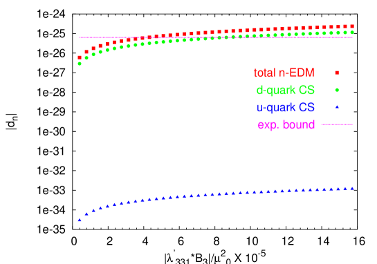
Figure 2: (color online) The neutron EDM (in units of e.cm) versus the combination $|B_{3}^{\ast}\lambda^{\prime}_{331}|$ normalized by $\mu_{\scriptscriptstyle 3}^{2}$. The charged scalar contribution (green dotted line) to the $d$ quark EDM is clearly seen to dominate over the charged-scalar $u$ quark EDM (blue dotted line). The total QCD corrected neutron EDM is shown in red line. The experimental upper bound is shown in pink dotted line.

In Fig.(2) we have plotted the neutron EDM versus the most important combination $|B_{3}^{\ast}\lambda^{\prime}_{331}|$ normalized by $\mu_{\scriptscriptstyle 0}^{2}$. As mentioned above, it can be clearly seen that the $d$ quark EDM contribution from the charged-slepton loop (green circles) dominates over the $u$ quark EDM (blue triangles). The experimental upper bound is shown with the pink horizontal dotted line and the QCD corrected total neutron EDM is shown in red squares. From the plot one can extract an upper bound of $4.0\cdot 10^{-5}$ on the combination of couplings $|B_{3}^{\ast}\lambda^{\prime}_{331}|/\mu_{\scriptscriptstyle 0}^{2}$. However this bound corresponds to a fixed value of relative phase ($\pi/4$) in the RPV parameter combination) as well as other supersymmetric parameters. Later in the table 1, we show the effects of variation in the major parameters. With a similar value of input parameters we obtain an upper bound of $2.2\cdot 10^{-4}$ for $|B_{3}^{\ast}\lambda^{\prime}_{321}|/\mu_{\scriptscriptstyle 0}^{2}$ and $8.4\cdot 10^{-4}$ for $|B_{3}^{\ast}\lambda^{\prime}_{311}|/\mu_{\scriptscriptstyle 0}^{2}$. The hierarchy in these bounds is due to the relevant CKM factors.

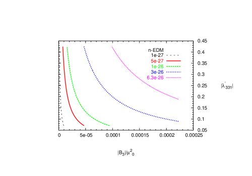
Figure 3: (color online) A contour plot for various values of neutron EDM in e.cm in the plane of real $\lambda^{\prime}_{331}$ and $B_{3}$. The red line is the present experimental bound for neutron EDM.

Fig.(3) shows the contours of neutron EDM in the plane of magnitudes for the couplings $\lambda^{\prime}_{331}$ and $B_{3}$ with the relative phase fixed at $\pi/4$. The contour for present experimental bound is shown in pink dotted line. The plot shows that a sizable region of the parameter space are ruled out. Successive contours show smaller values of neutron EDM with the smallest being $10^{-27}$ $e$ cm.

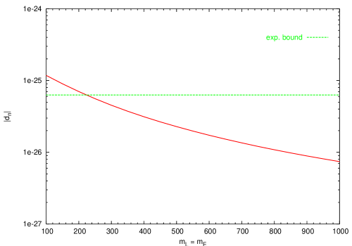
Figure 4: Neutron EDM vs. the slepton mass parameter ${\tilde{m}}_{L}={\tilde{m}}_{E}$ (with $|B_{3}|=200~{}\mbox{GeV}^{2}$, $|\lambda^{\prime}_{331}|=.05$ and relative phase of $\pi/4$). Horizontal line is the experimental bound.

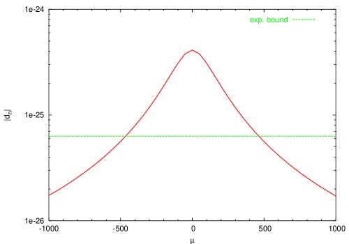
Figure 5: Neutron EDM vs. $\mu_{\scriptscriptstyle 0}$ parameter with $|B_{3}|=200~{}\mbox{GeV}^{2}$, $|\lambda^{\prime}_{331}|=.05$ and relative phase $\pi/4$. Horizontal line is the experimental bound.

So far we have kept certain parameters like the phase of the RPV combination, the $\mu_{\scriptscriptstyle 0}$ parameter and the slepton mass spectrum fixed. To get a better understanding of the allowed regions in the overall parameter space, let us focus on variations of the parameters one at a time. In Fig.(4) we have plotted neutron EDM versus the slepton mass parameter ${\tilde{m}}_{L}={\tilde{m}}_{E}$ (with $|B_{3}|=200~{}\mbox{GeV}^{2}$, $|\lambda^{\prime}_{331}|=.05$ and relative phase of $\pi/4$). As expected the neutron EDM falls with the increasing slepton mass. More careful checking reveals that the result is sensitive only to one slepton mass parameter, the mass of the third $L$-handed slepton here. It is also easy to understand from our analytical formulas that the dominating contributions among the various scalar mass eigenstates for the case of $B_{i}^{\ast}\lambda^{\prime}_{ijk}$ come from the $i$-th $L$-handed slepton and the Higgs. In Fig.(5) we have shown the variation of neutron EDM with the $\mu_{\scriptscriptstyle 0}$ parameter. Although parameter $\mu_{\scriptscriptstyle 0}$ does not directly figure in the EDM formula, its influence is felt through the Higgs spectrum. Larger $\mu_{\scriptscriptstyle 0}$ leads to heavier Higgs spectrum which suppresses the EDM contribution. As our analytical formulas show there is no strong dependence on $\tan\!\beta$ (we have checked this numerically as well) and hence we have kept $\tan\!\beta=3$ fixed in all the plots.

So far we have discussed only the combination $B_{i}^{\ast}\lambda^{\prime}_{i31}$ for the purpose of illustration. In table 1, we list the bounds on the nine combinations $|B_{i}^{\ast}\lambda^{\prime}_{ij1}|$ normalized by $(100~{}\mbox{GeV})^{2}$. It is interesting to note the difference in bounds for case (a) and (b) for coupling combination $|B_{i}^{\ast}\lambda^{\prime}_{i31}|$ and $|B_{i}^{\ast}\lambda^{\prime}_{i21}|$. The inputs for Case (b) are identical to case (a) except for RPV phase being zero for case (b). Case (b) thus relies solely on CKM phase. Interestingly the bound for $|B_{i}^{\ast}\lambda^{\prime}_{i31}|$ changes very marginally from case (a) to (b) whereas the bound for $|B_{i}^{\ast}\lambda^{\prime}_{i21}|$ weakens by about an order of magnitude. To understand this difference in behavior of $|B_{i}^{\ast}\lambda^{\prime}_{i31}|$ and $|B_{i}^{\ast}\lambda^{\prime}_{i21}|$, with and without a complex phase in the RPV couplings, we have plotted in Fig. 6 the allowed region in the plane of relative phase of $B^{\ast}_{3}\lambda^{\prime}_{331}$ and the $|B^{\ast}_{3}\lambda^{\prime}_{331}|$ (left) and relative phase of $B^{\ast}_{3}\lambda^{\prime}_{321}$ and the $|B^{\ast}_{3}\lambda^{\prime}_{321}|$ (right). One can see that the bound for $|B^{\ast}_{3}\lambda^{\prime}_{331}|$ is about the same for relative phase in $B^{\ast}_{3}\lambda^{\prime}_{331}$ of 0 or $\pi/4$ but the bound for $|B^{\ast}_{3}\lambda^{\prime}_{321}|$ strengthens by about an order of magnitude as the phase in the RPV coupling increases from 0 to $\pi/4$ suggesting a collaborative effect between the CKM phase and the RPV phase. For the case of $B_{i}^{\ast}\lambda^{\prime}_{i11}$ there is no CKM phase involved. In the table we have fixed the sign of $\mu_{\scriptscriptstyle 0}$ parameter to be negative. In the Fig. 5 it is seen that absolute value of neutron EDM is symmetric with respect to sign of $\mu_{\scriptscriptstyle 0}$ parameter and hence positive $\mu_{\scriptscriptstyle 0}$ should give identical bounds. The variation of bounds in table 1 with changes in parameters $\mu_{\scriptscriptstyle 0}$ and the slepton and Higgs mass very much follows the pattern found in plots discussed earlier.

parameter values					Normalized bounds
	$\mu_{\scriptscriptstyle 0}$	${\tilde{m}}_{\scriptscriptstyle L}$	$m_{{\scriptscriptstyle H}_{d}}$	RPV	$\frac{|B_{i}^{\ast}\cdot\lambda^{\prime}_{i31}|}{(100~{}\mbox{GeV})^{2}}$	$\frac{|B_{i}^{\ast}\cdot\lambda^{\prime}_{i21}|}{(100~{}\mbox{GeV})^{2}}$	$\frac{|B_{i}^{\ast}\cdot\lambda^{\prime}_{i11}|}{(100~{}\mbox{GeV})^{2}}$
				phase
(a)	-100 GeV	100 GeV	100 GeV	$\pi/4$	$1.6\cdot 10^{-4}$	$4.8\cdot 10^{-4}$	$2.0\cdot 10^{-3}$
(b)	-100 GeV	100 GeV	100 GeV	0	$1.8\cdot 10^{-4}$	$4.5\cdot 10^{-3}$	N.A.
(c)	-400 GeV	100 GeV	100 GeV	$\pi/4$	$5.0\cdot 10^{-4}$	$3.2\cdot 10^{-3}$	$1.1\cdot 10^{-2}$
(d)	-800 GeV	100 GeV	100 GeV	$\pi/4$	$1.7\cdot 10^{-3}$	$1.0\cdot 10^{-2}$	$3.7\cdot 10^{-2}$
(e)	-100 GeV	400 GeV	100 GeV	$\pi/4$	$6.5\cdot 10^{-4}$	$5.0\cdot 10^{-3}$	$1.8\cdot 10^{-2}$
(f)	-100 GeV	800 GeV	100 GeV	$\pi/4$	$2.0\cdot 10^{-3}$	$1.7\cdot 10^{-2}$	$5.8\cdot 10^{-2}$
(g)	-100 GeV	100 GeV	300 GeV	$\pi/4$	$4.9\cdot 10^{-4}$	$2.1\cdot 10^{-3}$	$7.5\cdot 10^{-3}$
(h)	-100 GeV	100 GeV	600 GeV	$\pi/4$	$1.1\cdot 10^{-3}$	$6.8\cdot 10^{-3}$	$2.4\cdot 10^{-2}$

Table 1: Here we list the normalized upper bounds for several combinations of bilinear and trilinear RPV parameters, with some variation in the input parameters. The bounds essentially depend on the values of parameters like ${\tilde{m}}_{\scriptscriptstyle L},\mu_{\scriptscriptstyle 0}$ and $m_{{\scriptscriptstyle H}_{d}}$ ($m_{{\scriptscriptstyle H}_{u}}$ and $B_{0}$ being determined from EW symmetry breaking condition). $\tan\!\beta$ has been kept fixed at 3 as EDM has a very mild dependence on $\tan\!\beta$.

Before we conclude, we would like to briefly comment on two things. In the table 1, we have only mentioned the bounds for the combinations $|B_{i}^{\ast}\lambda^{\prime}_{ij1}|$, whereas earlier in the text we did mention that in principle all the twenty-seven $\lambda^{\prime}_{ijk}$ together with bilinear couplings do contribute to the neutron EDM. The couplings other than $\lambda^{\prime}_{ij1}$ contribute to $u$ quark EDM and all the contributions are proportional to up-Yukawa (in contrast to the presence of a contribution proportional to top-Yukawa for the $d$ quark EDM). Strength of the corresponding contributions is substantially weaker (typically by 5 to 6 orders of magnitude) and hence do not lead to meaningful bounds. The other thing is about the possible $\mu_{i}^{\ast}\cdot\lambda^{\prime}_{ijk}$ contributions. It can be seen in Eq.(18) that these are second order in perturbation and also accompanied by lepton mass $\mu_{i}$. Thus, a typical $\mu_{i}^{\ast}\lambda^{\prime}_{ijk}$ contribution is substantially weaker than the corresponding $B_{i}^{\ast}\lambda^{\prime}_{ijk}$ contribution. For instance, with the similar inputs for other SUSY parameters as described above, if one takes $\mu_{3}=10^{-3}$ GeV (dictated by requirement of sub-ev neutrino masses), $\lambda^{\prime}_{331}=.05$ and a relative phase of $\pi/4$, one obtains neutron EDM of $6.0\cdot 10^{-32}$ which is about six orders of magnitude smaller than the present experimental bound on neutron EDM. If one goes by the upper bound on the mass of $\nu_{\tau}$ of 18.2 MeV [22], $\mu_{\scriptscriptstyle 3}$ could be as large as 7 GeV for $\tan\!\beta=2$ and sparticle mass $\sim 300$ GeV [19]. For $\mu_{\scriptscriptstyle 3}=1$ GeV we obtain neutron EDM of $6.1\cdot 10^{-29}$, still about three orders of magnitude smaller than the experimental bound. These numbers can be easily compared with the $\mu^{\ast}_{i}\lambda^{\prime}_{i11}$ contributions to the $d$ quark EDM through chargino loop in Table 1 of ref.[14]. There the corresponding contribution (with $\mu_{\scriptscriptstyle 3}=1$ GeV) is much weaker (of order $10^{-32}$) as it lacks the top Yukawa and top mass enhancements. In the same table one finds that corresponding contribution to gluino loop is much stronger (of order $10^{-25}$) due to proportionality to gluino mass and strong coupling constant. In the light of above reasons one can appreciate that the contributions due to soft parameter $B_{i}$ are far more dominating in the present scenario of quark loop contributions.

5 Conclusions

We have made a systematic study of the influence of bilinear and trilinear RPV couplings on the neutron EDM. A combination of bilinear and trilinear RPV is the only way RPV parameters can contribute at one loop level. RPV couplings contribute to both, $u$ quark as well as $d$ quark EDM. Such a contribution could come from charged-slepton Higgs mixing loop (contributing to both $u$ quark as well as $d$ quark EDM) or sneutrino-Higgs mixing loop (viable only for combination of nonzero $B_{i}\lambda^{\prime}_{i11}$ giving Majorana-like scalar mass insertion) contributing to only $d$ quark EDM. The class of diagrams all have a quark as the fermion running inside the loop. In our analytical expressions obtained based on perturbative diagonalization of the scalar mass-squared matrices, we demonstrated that charged-slepton Higgs mixing loop contribution to $d$ quark EDM far dominates the other contributions due to a diagram with the top-quark in the loop. In our numerical exercise we have obtained robust bounds on the combinations $\frac{|B_{i}^{\ast}\cdot\lambda^{\prime}_{ij1}|}{(100~{}\mbox{GeV})^{2}}$ for $i,j=1,2,3$ that have not been reported before. Even if the RPV couplings are real, they could still contribute to neutron EDM via CKM phase. For some cases CKM phase induced contribution is as strong as that due to an explicit complex phase in the RPV couplings. There also exist contributions involving $\mu_{i}^{\ast}\lambda^{\prime}_{ijk}$. However these are higher order effects which are further suppressed by proportionality to charged lepton mass. Since $\mu_{i}$ are expected to be very small (of order $10^{-3}$ GeV) for sub-eV neutrino masses, such contributions are highly suppressed. Our results presented here make available a new set of interesting bounds on combinations of RPV parameters.

Figure 1: $d$ quark EDM due to $B^{\ast}_{i}\lambda^{\prime}_{i31}$ combination. Due to top Yukawa and top-mass dependence this is the most dominant contribution.

Figure 6: Dotted region is the parameter space allowed by neutron EDM upper bound in the plane of relative phase of $\lambda^{\prime}_{331}B^{\ast}_{3}$ and the $|\lambda^{\prime}_{331}B^{\ast}_{3}|$ (left) and relative phase of $\lambda^{\prime}_{321}B^{\ast}_{3}$ and the $|\lambda^{\prime}_{321}B^{\ast}_{3}|$ (right).

References

- [1] J. H. Christenson, J. W. Cronin, V. L. Fitch, and R. Turlay, “Evidence for the 2 Decay of the Meson”, Phys. Rev. Lett. 13, 138 (1964).
- [2] B. Aubert et al. [BABAR Collaboration], “Observation of CP Violation in the B0 Meson System” Phys. Rev. Lett. 87, 091801 (2001); K. Abe et al. [Belle Collaboration], “Observation of Large CP Violation in the Neutral B Meson System” Phys. Rev. Lett. 87, 091802 (2001).
- [3] L. Landau, “On the Conservation Laws for Weak Interactions.” Nucl. Phys. 3, 127 (1957).
-
[4]
D. V Nanopoulous : on the electric dipole moment 2. M. B. Gavela et
al., (?)
M.E. Pospelov “CP-odd effective gluonic Lagrangian in the Kobayashi-Maskawa model“ Phys. Lett. B328 , 441 (1994); I.B. Khriplovich and A. R. Zhitnitsky, “What is the value of the neutron electric dipole moment in the Kobayashi-Maskawa model?” Phys. Lett. B109 , 490 (1982). - [5] P. G. Harris et al., “New Experimental Limit on the Electric Dipole Moment of the Neutron Phys. Rev. lett. 82, 904 (1999).
- [6] See, for example, T. Falk and K.A. Olive, “ More on electric dipole moment constraints on phases in the constrained MSSM” Phys. Lett. B439, 71 (1998), and references therein.
- [7] O.C.W. Kong, “On the Formulation of the Generic Supersymmetric Standard Model (or the Supersymmetry without R Parity)” Int. J. Mod. Phys. A19, 12 (2004).
- [8] For neutrino masses from R-parity Violation, see for example S. K. Kang and O. C. W. Kong “A Detailed Analysis of One Loop Neutrino Masses from the Generic Supersymmetric Standard Model”, Phys. Rev. D69, 013004 (2004); O. C. W. Kong “LR Scalar Mixings and One Loop Neutrino Masses” JHEP 0009,037 (2000); A. S. Joshipura, R. D. Vaidya and S. K. Vempati “Bimaximal and Bilinear R Violation”, Nucl. Phys. B639, 290 (2002); “Neutrino Anomalies in Gauge Mediated Model with Trilinear Violation”, Phys. Rev. D65, 053018 (2002).
- [9] A. S. Joshipura, R. D. Vaidya and S. K. Vempati “U(1) Symmetry and R-parity Violation”, Phys. Rev. D62, 093020 (2000).
- [10] For a review see, X.-G. He, B.H.J.Mckellar and S. Pakvasa “The Neutron Electric Dipole Moment” Int. J. Mod. Phys.A4, 5011 (1989).
- [11] Tarek Ibrahim and Pran Nath, “Neutron and electron electric dipole moment in N=1 supergravity unification” Phys. Rev. D57, 478 (1998); D60, 119901 (1999) ; D60, 079903 (1999) ; D58, 019901 (1998).
- [12] R. Arnowitt, Jorge L. Lopez, and D. V. Nanopoulos, “Electric dipole moment of the neutron in supersymmetric theories”, Phys. Rev. D42, 2423 (1990).
- [13] R. M. Godbole1, S. Pakvasa, S. D. Rindani, and X. Tata, “Fermion dipole moments in supersymmetric models with explicitly broken R parity” Phys, Rev. D 61, 113003 (2000); Steven A. Abel, Athanasios Dedes and Herbert K. Dreiner “Dipole moments of the electron, neutrino and neutron in the MSSM without R-parity symmetry” J. High Energy Phys.05, 013 (2000). Also see, Darwin Chang, We-Fu Chang, Mariana Frank, and Wai-Yee Keung, “Neutron electric dipole moment and CP-violating couplings in the supersymmetric standard model without R parity”, Phys. Rev. D62, 095002 (2000).
- [14] Y.-Y. Keum and O.C.W. Kong, “R-Parity Violating Contribution to the Neutron Electric Dipole Moment at One-Loop Order” Phys, Rev. Lett. 86, 393 (2001); “One-loop neutron electric dipole moment from supersymmetry without R parity” Phys, Rev. D 63, 113012 (2001).
- [15] Kiwoon Choi, Eung Jin Chun, Kyuwan Hwang, “Fermion electric dipole moments in supersymmetric models with R-parity violation”, Phys, Rev. D63, 013002 (2001).
- [16] O. C. W. Kong and R. D. Vaidya, “Some Novel contributions to Radiative B decays in Supersymmetry without R-parity” [arXiv: hep-ph/0408115]; see also Otto C. W. Kong and R. D. Vaidya, “Radiative B decays in Supersymmetry without R-parity” Phys. Rev. D71, 055003 (2005).
- [17] Kingman Cheung and O. C. W. Kong “ from Supersymmetry without R-parity” Phys. Rev. D64, 095007 (2001).
- [18] See for example Yoshiki Kizukuri and Noriyuki Oshimo “Neutron and electron electric dipole moments in supersymmetric theories”, Phys. Rev. D 46, 3025 (1992); Tarek Ibrahim and Pran Nath “Neutron and lepton electrifc dipole moments in the minimal supersymmetric standard model, large CP violating phases, and the cancellation mechanism”, Phys. Rev. D 58, 111301 (1998); Tomoko Kadoyoshi and Noriyuki Oshimo “Neutron electric dipole moment from supersymmetric anomalous W-boson coupling”, Phys. Rev. D 55, 1481 (1997) and references therein.
- [19] Mike Bisset, Otto C.W. Kong, Cosmin Macesanu, Lynne H. Orr, “A simple phenomenological parametrization of Supersymmetry without R-parity” Phys. Lett. B430, 274 (1998); “ Supersymmetry without R-parity: leptonic phenomenology”, Phys. Rev. D62, 035001 (2000).
- [20] M. Chemtob “Phenomenological Constraints on Broken R Parity Symmetry in Supersymmetry Models” Prog. Part. Nucl. Phys. 54, 71 (2005).
- [21] F. Ledroit, G. Sajot, GDR-S-008(1998).
- [22] R. Barate et al. , “An upper limit on tau neutrino mass from three prong and five prong tau decays”, Eur. Phys. J. C2, 395 (1998).