Dynamics and Decay of Heavy-Light Hadrons

Abstract

Recent signals for narrow hadrons containing heavy and light flavours are compared with quark model predictions for spectroscopy, strong decays, and radiative transitions. In particular, the production and identification of excited charmed and $c\bar{s}$  states are examined with emphasis on elucidating the nature of $0^{+}$ and $1^{+}$ states. Roughly 200 strong decay amplitudes of $D$ and $D_{s}$ states up to 3.3 GeV are presented. Applications include determining flavour content in $\eta$ mesons and the mixing angle in $P$ and $D$ wave states and probes of putative molecular states. We advocate searching for radially excited $D_{s}^{*}$ states in $B$ decays.

I Introduction

The discovery of the $D_{s}(2317)$ $(0^{+})$ and $D_{s}(2460)$ $(1^{+})$ mesonsdsstates ; PDG , with masses considerably lower than expected in potential modelsGI , stimulated a range of theoretical activity. The current knowledge of charmed and $c\bar{s}$  mesons, compared to the expectations of Ref GI is summarised in Figs. 1,2 for the $D$ and $D_{s}$ systems respectively. There is a significant amount of consistency between theory and experiment, interspersed with additional states that do not fit well into such a classification, of which the $D_{s}(0^{+})$ and $D_{s}(1^{+})$ are particularly sharp examples. Attempts to accommodate these states have invoked a variety of mechanisms. One interpretation is that they are indeed $q\bar{q}$${}^{3}P_{J}$ levels, with their low masses being a realisation of chiral symmetry such that $m(0^{+})-m(0^{-})\equiv m(1^{+})-m(1^{-})$chiral . An alternative is that they are multiquark or molecular configurations bcl associated with the $DK$ and $D^{*}K$ thresholds. One unresolved issue in the latter class of models is whether there are also further $(0,1)^{+}$ broad $c\bar{s}$  states above $D^{(*)}K$ threshold, analogous to what appears to occur with light flavoured scalar mesonsCT02 . To help decide among competing interpretations, a coherent study of the dynamics of heavy-light hadrons is merited.

A particular issue in testing these hypotheses will be to determine the ${}^{3}P_{1}-{}^{1}P_{1}$ mixing angle for the axial mesons. In the chiral symmetry picturechiral this is implicitly assumed to be the ideal heavy quark limit (see Section III.2). In the molecular picture it is moot whether there is any simple mixing angle involving the $D_{s}(2460)$ and $D_{s}(2535)$ or whether a further axial with mass $\sim 2.5$GeV is called for.

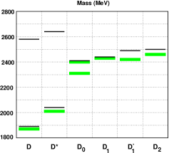
Figure 1: $D$ Spectrum. The lines are predictions from Ref. GI ; the boxes are data PDG . Both the Belle and Focus $D_{0}$ states are shown belle .

Subsequent to the above discoveries, SELEXselex reported a narrow state $D_{s}(2632)$ seen in $D_{s}\eta$ and $DK$ with a branching ratio $D_{s}(2632)\to D_{s}\eta\sim 6DK$. The narrow width and the anomalous branching ratios (the two channels share the same quark flavours and phase space favours the $DK$ mode over the $D_{s}\eta$) led to suggestions that this state may be a tetraquarkmaiani . Within the more conservative $c\bar{s}$  picture it was noted that the radially excited $2^{3}S_{1}$ is predicted to lie at $\sim 2.73$ GeV and that the presence of nodes in the wavefunction could lead to suppression of certain modes if the decay momentum coincides with a node in momentum spacebcdgs . Such dynamics have been applied to the decays of excited $c\bar{c}$  statesexcitedcc and also to light flavours with some successBarnes:1996ff ; however, Ref.bcdgs found that such an explanation would only work if extreme values for the parameters were chosen and thereby concluded that the SELEX state might be an artefact. While we still agree with that conclusion, it does raise the possibility that narrow states could in principle occur if their masses and decay kinematics cause the momenta to coincide with nodes; this is one of the questions that we pursue in this survey.

Independent of these tantalising possibilities, the transitions among excited hadrons can determine their dynamics and discriminate among models. With the production of charm in B decays, and the possible advent of charm factories at CLEO-c and GSI, it is timely to assess the landscape for heavy-light hadrons.

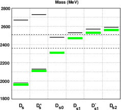
Figure 2: $D_{s}$ Spectrum. See Fig. 1.The dashed lines are the $DK$ and $D^{*}K$ thresholds.

Some highlights of the results are as follows:

Significant production of $D_{s}(2^{3}S_{1})$ and $D_{s}(3^{3}S_{1})$ is predicted in B decays. Similarly, B decays may be a significant source of $D_{1}$ mesons and can be used to test axial mixing.

Decay ratios such as ${D_{s}^{*}}^{\prime}\to D_{s}\eta$/${D^{*}}^{\prime}\to D\eta$ are useful probes of the flavour structure of the $\eta$ meson.

The decays ${D_{s}^{*}}^{\prime\prime}\to D_{s1}\eta$ and $D_{s1}^{\prime}\eta$ test the putative molecular nature of the $D_{s}(2460)$. Similarly, the decays $D_{S}^{\prime\prime}\to D_{s0}\eta$, $D^{\prime\prime}\to D_{s0}K$, and ${D_{s}^{*}}^{\prime\prime}\to D_{s0}K^{*}$ probe the structure of the enigmatic $D_{s}(2317)$.

There may be considerable spectroscopic mixing between the $D_{s}(2^{3}S_{1})$ and $D_{s}(^{3}D_{1})$ states which can be tested by measuring the transitions to $DK$ and $DK^{*}$ from the vector $D_{s}$ states.

E1 transitions such as $2^{3}S_{1}\to{}^{1}P_{0,1}$ are useful probes of the $D_{1}$ and $D_{s1}$ mixing angles.

Novel radiative transition selection rules are obtained in the heavy quark limit.

Radiative transitions such as $1^{+}\to 0^{+}\gamma$, $0^{+}\to 1^{-}\gamma$, $1^{+}\to 0^{-}\gamma$ can test molecular models in the $c\bar{s}$ sector. For example, the width of the intermolecular transition $1^{+}\to 0^{+}\gamma\sim 17$ keV contrasts with the ${\cal O}(1)$ keV rate predicted for $c\bar{s}$  states.

Anomalous branching ratios of excited states, for example, $D_{s}^{\prime\prime}\to D_{2}K$ being much larger than $D^{*}K$ or $DK^{*}$, may be used to probe the nodal structure of hadron wavefunctions.

We proceed with a description of the strong decay model and the conventions concerning state mixing. This is followed by a discusson of the phenomenology of the strong decay results and their relationship to the heavy quark limit. The penultimate section concerns radiative transitions and highlights their utility as a diagnostic tool. All transition rates are contained in Appendices B and C; Tables 4, 5, and 6 for radiative transitions and Tables 7–14 for strong transitions.

II Method

II.1 The Decay Model

The ${}^{3}P_{0}$ model of strong decays assumes that $q\bar{q}$ pairs are created with vacuum quantum numbersMicu:1968mk . Thus the interaction may be written as

$$H_{q\bar{q}}=\gamma\,\sum_{f}2m_{f}\int d^{\,3}x\;\bar{\psi}_{f}\psi_{f}\ ,$$ (1)

where $\psi_{f}$ is a Dirac quark field of flavour $f$, $m_{f}$ is the constituent quark mass, and $\gamma$ is a dimensionless $q\bar{q}$pair production strength.

Recent variants of the ${}^{3}P_{0}$ model consider modifications of the pair-production vertex Roberts:1997kq , or assume that pair creation originates in a gluonic flux tubeKokoski:1985is . The latter is the “flux-tube decay model”, which in practice gives very similar predictions to the ${}^{3}P_{0}$ model.

The model has been extensively applied to meson and baryon strong decays, with considerable successapplications ; Barnes:1996ff ; Godfrey:1986wj . The pair-production strength parameter $\gamma$ is fitted to strong decay data, and is roughly flavor-independent for decays involving production of $u\bar{u}$, $d\bar{d}$ and $s\bar{s}$ pairs. A typical value obtained from computation of light meson decays is $\gamma=0.4$Ackleh:1996yt ; Barnes:1996ff ; Barnes:2002mu , assuming simple harmonic oscillator (SHO) wavefunctions with a global scale, $\beta=0.35$ – $0.4$ GeV. The present work also assumes SHO wavefunctions but applies the formalism to a variety of heavy-light mesons; thus we have allowed the SHO $\beta$ values to vary according to the state (see Table 2 in Appendix A). These values were obtained by equating the root mean square (RMS) radius of the SHO wavefunction to that obtained in a simple nonrelativistic quark model with Coulomb+linear and smeared hyperfine interactions. Details are provided in the Appendix.

In view of this it is appropriate to refit experimental data to obtain a new value for the coupling, $\gamma$. A total of 32 experimentally well-determined decay rates have been fit with the model. Several variations of the decay model were also examined. Details and the final parameters and method are discussed in Appendix A.

II.2 Mixed States

Heavy-light mesons are not charge conjugation eigenstates and so mixing can occur among states with the same $J^{P}$ that are forbidden for neutral states. These occur between states with $J=L$ and $S=1$ or $0$. For example the $J^{P}=1^{+}$ axial vector $c\bar{n}$ and $c\bar{s}$ mesons $\rm D_{1}$ and $\rm D_{1}^{\prime}$ are coherent superpositions of quark model ${}^{3}P_{1}$ and ${}^{1}P_{1}$ states,

$$|\rm D_{1}\rangle =+\cos(\phi)|^{1}\rm P_{1}\rangle+\sin(\phi)|^{3}\rm P_{1}\rangle$$ (2)

$$|\rm D_{1}^{\prime}\rangle =-\sin(\phi)|^{1}\rm P_{1}\rangle+\cos(\phi)|^{3}\rm P_{1}\rangle.$$

Quantifying the mixing pattern as a function of flavour will give information about the internal dynamics; little is known empirically at present. In the heavy quark limit $M_{Q}\to\infty$ there is an explicit prediction for the mixing angle assuming that it is generated by spin-orbit interactions (see Section III.2). One of our aims will be to devise tests for determining this mixing in practice for heavy, but finite flavour masses.

Mixing between $S=0,1$ states with the same $J$ also occurs for ${}^{3}D_{2}$ and ${}^{1}D_{2}$ states:

$$|D_{2}^{*}\rangle = +\cos(\phi_{D})|^{1}D_{2}\rangle+\sin(\phi_{D})|^{3}D_{2}\rangle$$

$$|{D_{2}^{*}}^{\prime}\rangle = -\sin(\phi_{D})|^{1}D_{2}\rangle+\cos(\phi_{D})|^{3}D_{2}\rangle$$ (3)

Kokoski and GodfreyGodfrey:1986wj find the angles (these supersede those of Ref. GI ) $\phi(1P_{cu})=-26$ degrees and $\phi(1P_{cs})=-38$ degrees, upon converting their mixing conventions to ours. $D$-wave mixing angles were not computed.

Finally, the physical $\eta$ and $\eta^{\prime}$ are taken to be

$$\eta = +\cos(\theta){1\over\sqrt{2}}(u\bar{u}+d\bar{d})+\sin(\theta)s\bar{s}$$

$$\eta^{\prime} = -\sin(\theta){1\over\sqrt{2}}(u\bar{u}+d\bar{d})+\cos(\theta)s\bar{s}.$$ (4)

A typical quark model $\eta$ mixing angle is $\theta=-45$ degrees. See Section III.5 for further discussion on how to interpret the amplitudes for $\eta$ production.

III Strong Decays

We proceed with a discussion of OZI allowed strong decays of $D$ and $D_{s}$ states.

III.1 1S States

$D^{*}$ decays are interesting because the open channels are so close to threshold that isospin symmetry breaking mass shifts become important. In particular $D^{*+}$ may decay to both $D^{0}\pi^{+}$ and $D^{+}\pi^{0}$, but the $D^{\pm}\pi^{\mp}$ mode of $D^{*0}$ is closed. The experimental $D^{*+}$ widths are in the ratio

$${\Gamma(D^{*+}\to D^{0}\pi^{+})\over\Gamma(D^{*+}\to D^{+}\pi^{0})}=2.21\pm 0.57.$$ (5)

The final state relative momenta are $q=0.0393$ GeV and $q=0.0379$ GeV respectively, thus the form factor is essentially unity, the ratio is dominated by the isospin factor and is predicted to be 2.28.

Absolute rates are given in Table 7 where one sees that the $D^{*+}$ widths are under-predicted by a factor of three. This is the largest error we have encountered with the ${}^{3}P_{0}$ model; for example the analogous decay $K^{*}\to K\pi$ is under-predicted by approximately 45% in amplitude. While this would be easy to correct by adjusting the ${}^{3}P_{0}$ coupling, we choose to retain the fit value of Appendix A since it does well globally. We note that the decay model is tuned for SHO wavefunctions and decays of momenta of hundreds of MeV. Thus it is perhaps no surprise that the largest error seen in the ${}^{3}P_{0}$ model is seen in this extreme, near-threshold, decay.

III.2 P-waves

It is convenient to discuss heavy-light mesons in the $jj$ coupling scheme. One has $L_{J}=s_{1/2}$ for the heavy quark which must combine with the light quark spin and angular momentum to form a total $J^{P}$ state. In the P-waves $\ell_{j}=P_{1/2}$ and $P_{3/2}$. Thus the $j=1/2$ states form a doublet with $J^{P}=(0,1)^{+}$ while the $j=3/2$ states form a $J^{P}=(1,2)^{+}$ doublet.

The relationship of these states to those in the $LS$ coupling scheme can be determined once the heavy quark dynamics has been isolated and conventions have been fixed. We chose to employ the conventions of Ref.Barnes:2002mu . This reference also discusses the other conventions for the mixing angle that have appeared in the literature. In the heavy-quark limit a particular “magic” mixing angle follows from the quark mass dependence of the spin-orbit and tensor terms, which is $\phi_{HQ}=-54.7^{o}$ $(35.3^{o})$ if the expectation of the heavy-quark spin-orbit interaction is positive (negative) Godfrey:1986wj . Since the former implies that the $2^{+}$ state is greater in mass than the $0^{+}$ state, and this agrees with experiment, we employ $\phi=-54.7^{o}$ in the following. This implies

$$|P_{1}\rangle_{HQ} = +{1\over\sqrt{3}}|^{1}P_{1}\rangle-\sqrt{2\over 3}|^{3}P_{1}\rangle$$

$$|P_{1}^{\prime}\rangle_{HQ} = +\sqrt{2\over 3}|^{1}P_{1}\rangle+{1\over\sqrt{3}}|^{3}P_{1}\rangle.$$ (6)

In practice the empirical mixing for the $D$ and $D_{s}$ systems is not yet known. Quantifying this is one of the challenges that we discuss here for both $c\bar{s}$and $c\bar{q}$systems. For example, our decay model makes specific predictions for certain amplitude ratios:

$${\cal A}({}^{1}P_{1}\to VPs)_{S} = -{1\over\sqrt{2}}{\cal A}({}^{3}P_{1}\to VPs)_{S}$$ (7)

$${\cal A}({}^{1}P_{1}\to VPs)_{D} = \sqrt{2}{\cal A}({}^{3}P_{1}\to VPs)_{D}$$ (8)

$${\cal A}(2{}^{3}S_{1}\to{}^{1}P_{1}Ps)_{S} = -{1\over\sqrt{2}}{\cal A}(2{}^{3}S_{1}\to{}^{3}P_{1}Ps)_{S}$$ (9)

$${\cal A}(2{}^{3}S_{1}\to{}^{1}P_{1}Ps)_{D} = \sqrt{2}{\cal A}(2{}^{3}S_{1}\to{}^{3}P_{1}Ps)_{D}$$ (10)

$${\cal A}({}^{3}D_{1}\to{}^{1}P_{1}Ps)_{S} = \sqrt{2}{\cal A}({}^{3}D_{1}\to{}^{3}P_{1}Ps)_{S}$$ (11)

which underpin the eventual extraction of the mixing angles. These relationships imply that the heavy quark $P_{1}$ state of Eq. 6 couples to $VPs$ in $S$-wave, whereas the $P_{1}^{\prime}$ heavy quark state couples in $D$-wave. Thus one expects the $D_{1}$ (${D_{1}}^{\prime}$) to be broad (narrow) in the heavy quark limit. Similarly, Eq. 11 implies that the the $D_{1}\pi$ ($D_{1}^{\prime}\pi$) mode will be large (small) in $2{}^{3}S_{1}$ decays and the $D_{1}\pi$ ($D_{1}^{\prime}\pi$) mode will be small (large) in ${}^{3}D_{1}$ decays.

Table 7 give the predicted widths of the $D_{1}$ and $D_{1}^{\prime}$ states in terms of the mixing angle ($c$ denotes $\cos\phi$). Equating these to the measured rates of $329\pm 84$ MeV and $19\pm 5$ MeV gives very good fits for mixing angles of $\phi\approx-55^{o}$ or $35^{o}$. The first angle is the solution for a broad $D_{1}$ while the second is for a broad $D_{1}^{\prime}$. Since these correspond to $-54.7^{o}$ and $+35^{o}$ respectively, good agreement is obtained with the heavy quark predictions, although distinguishing the two scenarios is impossible. This agreement may be tested by measuring decays with $D_{1}$s in the final state. The decay tables indicate that the most promising such decays are $D(^{3}D_{1})\to D_{1}\pi$ and $D_{1}^{\prime}\pi$, ${D^{*}}^{\prime\prime}\to D_{1}\pi$ and $D_{1}^{\prime}\pi$, and ${D_{s}^{*}}^{\prime\prime}\to D_{1}K$ and $D_{1}^{\prime}K$.

The situation for the $D_{s1}$ is less satisfactory because both the $D_{s1}$ and $D_{s1}^{\prime}$ states are expected to be narrow due to the limited phase space available for the $D^{*}K$ channel. The heavy quark ${}^{3}P_{0}$ model prediction for the $D_{s1}^{\prime}$ width is 800 keV. Model uncertainties can be removed by measuring the ratio

$${\Gamma(D_{s1}^{\prime}\to D^{*}K)\over\Gamma(D_{s2}\to D^{*}K)}=84\cos^{2}\phi_{s}+42\sin^{2}\phi_{s}-119\cos\phi_{s}\sin\phi_{s}.$$ (12)

The $D_{s1}$ mixing angle may also be accessed through the decays ${D^{*}}^{\prime\prime}\to D_{s1}K$ and $D_{s1}^{\prime}K$ and ${D_{s}^{*}}^{\prime\prime}\to D_{s1}\eta$ and $D_{s1}^{\prime}\eta$ although only the $D_{s1}K$ mode presents a substantial branching fraction.

The $1^{+}$ $c\bar{s}$  states can be directly produced by the $W$ axial current in $B\to\bar{D}D_{s1}$ or $\bar{D}D_{s1}^{\prime}$od , thus B factories offer the possibility of studying these intriguing states. However, heavy quark symmetry suppresses the $P_{3/2}$ $1^{+}$ decay constantors so that production of the $D_{s1}^{\prime}$ may be negligible. Furthermore there is no conserved vector current suppression of the scalar $c\bar{s}$  due to the different masses of the $c$ and $\bar{s}$ in such transitions and hence the $D_{s0}$ may also be detectable. The relative production of these states in $B$ decays will provide further insight into the relationship between the various $c\bar{s}$  states with $J^{P}=0^{+},1^{+}$. For example, the enigmatic $D_{s0}$ is produced in $D^{\prime\prime}$ and ${D^{*}}^{\prime\prime}$ decays to $D_{s0}K$ and $D_{s0}K^{*}$ respectively; with the former having a branching fraction of approximately 17%. This is sufficiently large that it may worth looking for. One expects that these branching fractions would be substantially lower if the $D_{s0}$ state were a molecule.

In addition to the curious $J^{P}=0^{+}$ and $1^{+}$ states in the $c\bar{s}$  system, there are also questions in the charmed $D$ states. A simple problem is the existence of incompatible candidates for the $0^{+}$ states at 2308 and 2407 MeVbelle . The $c\bar{d}$  state may be produced directly in $B$ decay as above, but with the additional penalty of Cabibbo suppression. It is also possible to produce the $D_{0}$ in $D^{\prime\prime}$ and $D_{s}^{\prime\prime}$ decays.

Finally, as noted in the Introduction, it has been suggested that the anomalously low masses of the $D_{s}(2317)$ and $D_{s}(2460)$ are consistent with breaking heavy quark and chiral symmetrychiral . This implies $m(0^{+})-m(0^{-})\equiv m(1^{+})-m(1^{-})$. Presumably this relationship applies to $s_{1/2}$ and $p_{1/2}$ states and hence the mass of the broad $D_{(s)1}$ state should employed. For the $D_{s}$ system one obtains 349 MeV and 347 MeV for the left and right sides of the equation. Although not considered by the authors of Ref. chiral , in principle this relationship applies to the $D$ system as well. The $J=1$ mass difference is measured to be 347 MeV and the $J=0$ mass difference is 349 MeV if the lighter Belle $D_{0}$ mass is used. Thus, if taken seriously, this relationship supports the Belle results. We stress that it is important to test the applicability of this model through measurements of other observables, including the $P_{1}$ mixing angle.

III.3 2S and 1D waves

All $J^{P}$ combinations of $D^{*}$ can be produced in decays such as $B\to D^{*}\ell\nu$, and the hadronic analogues, though transitions to states where the light degrees of freedom are in highly excited states will be suppressed by poor wavefunction overlaps and restricted phase space. The production of excited $1^{-}$ and $0^{-}$ should be feasible as they can be emitted from the $W$ in weak transitions such as $B\to D_{s}^{(*)}\bar{D}$: the form factor that is relevant here is driven by the wavefunction at short distances. A simple quark model computation confirms that the wavefunction at the origin is not strongly suppressed as the principle quantum number increases, and the recoil momentum is sufficiently low that there is very little dependence on the $B\to D$ transition form factor. Thus, the rate $B\to D_{s}^{*}(n)\bar{D}$ depends primarily on the phase space and one finds that the relative emission rates are

$$B\to D_{s}^{*}\bar{D}:B\to{D_{s}^{*}}^{\prime}\bar{D}:B\to{D_{s}^{*}}^{\prime\prime}\bar{D}\approx 1:0.35:0.03$$ (13)

As the branching ratio $b.r.(B\to D_{s}^{*}\bar{D})$ and $b.r.(B\to D_{s}^{*}\bar{D}^{*})$ are each approximately 1%PDG one expects a total production of $2^{3}S_{1}({D_{s}^{*}}^{\prime})$ at roughly 1%. And even the doubly excited $D_{s}^{*}$ will have a branching fraction of order $10^{-3}$. The charmed analogue $2^{3}S_{1}({D^{*}}^{\prime})$ is Cabbibo suppressed and can be expected at the $10^{-3}$ level. As noted in the previous Section, the axial and scalar $c\bar{s}$  states can be produced in this way. For example, the $0^{-}$ $D_{s}^{\prime}$ can also be produced; its decay is predicted to be almost entirely into $D^{*}K$. We therefore advocate that these states should be sought at high statistics $B$-factories.

The signatures for the vector states are as follows. The $c\bar{s}$  $2^{3}S_{1}({D_{s}^{*}}^{\prime})$ decays dominantly to $D^{*}K(80\%)$ and $DK(15\%)$ with traces of $D_{s}\eta$ and $D_{s}^{*}\eta$. The $D_{1}K$ channel is closed; to access the $D_{1}$ this way requires the $3^{3}S_{1}$ initial state (see the discussion in the next section). The charmed $2^{3}S_{1}({D^{*}}^{\prime})$ decays dominantly to $D_{1}\pi(75\%)$ and $D^{*}\pi(10\%)$ with traces of $D\pi$ and $D^{*}\eta$.

The first excited vector ${D_{s}^{*}}^{\prime}$ and ${D^{*}}^{\prime}$ arise in either $2^{3}S_{1}$ or $1^{3}D_{1}$ configurations and in general there can be mixing between these. Such mixing will tend to shift the masses of the eigenstates away from the simple potential model values of Figs. 1,2. The unperturbed masses for $D_{s}^{*}$ of $2^{3}S_{1}(2.73)$ or $1^{3}D_{1}(2.90)$ imply that one of these eigenstates will be kinematically forbidden to decay to $D(1P)K$ while the other will be allowed. In the latter case there are interesting nodal effects, whose character will depend on the mixing angle.

Similar remarks hold for the $c\bar{q}$  states and the decays to $D(1P)\pi$. However in this case the small pion mass implies that the $D(1P)\pi$ channel may be open for both initial states. The role of decays of these states in determining the $1^{+}$ mixing angles by decays to $1^{+}0^{-}$ was discussed in Section III.2.

The $0^{+}$ 1P state is clearly $Qp_{1/2}$, so there is no mixing problem with this final state in the transition from $2S(0^{-})\to 0^{+}0^{-}$. Thus the $0^{+}$ may be accessed via this transition from a $D_{s}(2S)$ produced in B decay. So given a $D_{s}(2S)$ emitted from the W current in B decay, one may access the $0^{+}$ state by the above transition. However, the analogous $D^{\prime}$ production is Cabibbo suppressed and it decays dominantly to $D^{*}\pi$; the $D_{s}^{\prime}$ analogously decays to $D^{*}K$. It would be interesting to study transitions to the analogous $D_{s}$ states and determine whether the $D_{s}(2317)$ and $D_{s}(2460)$ are $c\bar{s}$  or other compounds. This would require the initial state to be 3S in order to be kinematically open.

Mixing in the ${}^{3}D_{2}-{}^{1}D_{2}$ system may be addressed in the heavy quark limit of the constituent quark model. Diagonalising the the spin-orbit interaction yields the results

$$M(^{3}D_{1}) = M(D_{2}^{*})=M_{0}-{3\over 2}\langle H_{SO}^{q}\rangle_{D}$$ (14)

$$M(^{3}D_{3}) = M({D_{2}^{*}}^{\prime})=M_{0}+\langle H_{SO}^{q}\rangle_{D},$$

and a ${}^{3}D_{2}-{}^{1}D_{2}$ mixing angle of $\phi_{D}=-50.76^{o}$. Thus, the heavy quark $D$-wave states are

$$|D_{2}^{*}\rangle_{HQ} = \sqrt{2\over 5}|^{1}D_{2}\rangle-\sqrt{3\over 5}|^{3}D_{2}\rangle$$

$$|{D_{2}^{*}}^{\prime}\rangle_{HQ} = \sqrt{3\over 5}|^{1}D_{2}\rangle+\sqrt{2\over 5}|^{3}D_{2}\rangle.$$ (15)

As with $P$-waves, the ${}^{3}P_{0}$ strong decay model makes specific predictions for $D$-wave heavy quark decay amplitudes which may be useful in interpreting the spectroscopy. Some of these are:

$${\cal A}({}^{1}D_{2}\to VPs)_{P} = -\sqrt{2\over 3}{\cal A}({}^{3}D_{2}\to VPs)_{P}$$ (16)

$${\cal A}({}^{1}D_{2}\to VPs)_{F} = +\sqrt{3\over 2}{\cal A}({}^{3}D_{2}\to VPs)_{F}$$ (17)

$${\cal A}({}^{1}D_{2}\to{}^{1}P_{1}Ps) = 0$$ (18)

The second of these is an example of the ${}^{3}P_{0}$ selection rule forbidding such transitions among $q\bar{q}$spin singletsfcpage .

We note that, in analogy with the $P$-waves, the amplitude ratios above imply that the $D_{2}^{*}$ decays strongly in $P$ wave while the ${D_{2}^{*}}^{\prime}$ decays only in $F$ wave and is thus narrower than the $D_{2}^{*}$. As with $P$-waves, this conclusion agrees with spin conservation in the heavy quark limit. Unfortunately, the ability to distinguish the states is weakened by the many other decay modes which exist for these states. Nevertheless, the $D_{2}^{*}$ and ${D_{2}^{*}}^{\prime}$ have total widths which depend strongly on $\phi_{D}$ and measurement of any (or several) of the larger decay modes will provide (over) constrained tests of the model and measurements of the mixing angle.

Finally we note that the transitions ${}^{1}D_{2}\to VV$ and ${}^{3}D_{2}\to VV$ proceed in ${}^{3}P_{2}$, ${}^{5}P_{2}$, ${}^{3}F_{2}$, and ${}^{5}F_{2}$ waves, but never share a wave. Thus there is no ${}^{1}D-{}^{3}D$ mixing due to $VV$ loops.

The effects of wavefunction nodes can be seen in Figs. 3 and 4. Here the partial widths are plotted for fixed $\beta$ as a function of the mass of the initial state. For the ${D_{s}^{*}}^{\prime}$, nodes would significantly affect the total width if the mass were roughly 3.1 MeV. Alternatively, nodes directly affect the width of the $D_{s}^{\prime\prime}$ by suppressing the $D^{*}K$, $DK^{*}$, and $D^{*}K^{*}$ modes while enhancing the $D_{2}K$ mode. The figure indicates that a $D_{s}^{\prime\prime}$ at 3.3 GeV would have a substantial branching fraction to $D^{*}K^{*}$ while one at 3.4 GeV would have no $D_{2}K$ mode. Clearly these effects must be accounted for in the phenomenology of heavy-light mesons.

Figure 3: ${D_{s}^{*}}^{\prime}$ Partial Widths vs. Mass. The arrow shows the nominal mass of the ${D_{s}^{*}}^{\prime}$.

Figure 4: ${D_{s}}^{\prime\prime}$ Partial Widths vs. Mass. The arrow shows the nominal mass of the ${D_{s}}^{\prime\prime}$.

III.4 3S and 2D waves

Similar remarks apply here as to the $2S$ waves with the bonus that phase space for decays into the $1P$ states is open leading to potential measures of the axial mixing angle (Tables 11 and 14). The challenge is to produce a significant sample of these $3S$ states in $B$-decays. Our estimate of the branching ratio $b.r.(B\to D_{s}^{*^{\prime\prime}}[\bar{D}+\bar{D}^{*+}])\sim 10^{-3}$ suggests that this may be feasible. Decays to $D_{1}X$ are predicted to be $\sim 50\%$, which may provide a significant source of the axial charmed mesons and a measure of their mixing. Decays to $D_{s1}\eta$ and $D^{\prime}_{1s}\eta$ may also be measured and used to test if the $D_{s}(2460)$ is the $c\bar{s}$  partner of the $D_{s1}(2535)$ or an independent state such as a $D^{*}K$ molecule.

The decays of $D_{s}^{\prime\prime}$ and ${D_{s}^{*}}^{\prime\prime}$ can access the enigmatic $D_{s}(2317)$ and $D_{s}(2460)$. For example, comparison of the predicted rates for ${D_{s}^{*}}^{\prime\prime}\to D_{s1}\eta$ and ${D_{s}^{*}}^{\prime\prime}\to D_{s1}^{\prime}\eta$ will test the putative $c\bar{s}$  nature of the axial states.

In the charm $D$ system the decays ${D_{s}^{*}}^{\prime\prime}\to D_{1}K$, $D_{1}^{\prime}K$ and $D_{2}K$ measure the axial mixing angles. A robust prediction of the model is that the sum of the two axial decay modes should be roughly $7.8$ times as large as the $D_{2}K$ mode.

Finally, the status of $D_{0}(2308)$ and $D_{0}(2407)$ candidates may be tested by searching for them in the $D_{0}\pi$ and $D_{0}\eta$ decay modes of the $D^{\prime\prime}$ where they have a non-negligible branching fraction.

III.5 Probing the $\eta$ system

The emission of an $\eta$ in $2S\to 1S$ transitions is kinematically allowed, while $\eta^{\prime}$ emission is forbidden. Alternatively both are permitted in $3S\to 1S$ transitions. We note that the flavour flow in the $D$ and $D_{s}$ systems probes the quark content of the $\eta$’s. Thus $\eta$’s are produced via their $n\bar{n}$ content in the $c\bar{q}$ system, whereas in $c\bar{s}$  decays it is the $s\bar{s}$ components that are involved.

Thus a comparison of $c\bar{q}$  $\to\eta$+$c\bar{q}$  and $c\bar{q}$ $\to\pi+$$c\bar{q}$ probes the $n\bar{n}$   content weighted by phase space and form factor effects. A rather direct measure of the $n\bar{n}$ vs. $s\bar{s}$ content of the $\eta$ can be obtained by comparing

$$\Gamma\left(D^{*}(2S)\to D(1S)\eta(n\bar{n})\right):\Gamma\left(D_{s}^{*}(2S)\to D_{s}(1S)\eta(s\bar{s})\right)$$

or

$$\Gamma\left(D(2S)\to D^{*}(1S)\eta(n\bar{n})\right):\Gamma\left(D_{s}(2S)\to D_{s}^{*}(1S)\eta(s\bar{s})\right).$$

though the predicted branching ratios are small.

The predictions in Appendix C for $\eta$ and $\eta^{\prime}$ production assume that these states are equally weighted mixtures of $n\bar{n}$   and $s\bar{s}$ . Hence with conventions for the $\eta$ wavefunction specified above, the amplitude ratio $D_{s}\to D_{s}\eta$ and $D\to D\eta$ is $\sqrt{2}\tan{\theta}$. This is modified by different wavefunctions, different quark masses, and different meson masses. Direct computation gives the factors shown in Table 1; these should be multiplied by $\sqrt{2}\tan{\theta}$ to obtain physical amplitude ratios. Determining several of these amplitude ratios will provide a constrained measure of the mixing angle and the efficacy of the decay model.

Table 1: Amplitude ratios probing $\eta$ decays with $\sqrt{2}\tan{\theta}$ removed.

${{D_{s}^{*}}^{\prime}\to D_{s}\eta\over{D^{*}}^{\prime}\to D\eta}$	${{D_{s}^{*}}^{\prime}\to D_{s}^{*}\eta\over{D^{*}}^{\prime}\to D^{*}\eta}$	${D_{s2}^{*}\to D_{s}\eta\over D_{2}^{*}\to D\eta}$	${D_{s}^{\prime}\to D_{s}^{*}\eta\over D^{\prime}\to D^{*}\eta}$
1.78	0.918	1.09	0.483

IV Radiative Transitions

Radiative transitions probe the internal charge structure of hadrons and are therefore useful in determining hadronic structure. In particular they can help distinguish possible exotic molecular or tetraquark state interpretations of the $D_{s}(0^{+})$ and $D_{s}(1^{+})$ and determine mixing angles.

IV.1 E1 and M1 Transitions

E1 radiative partial widths are evaluated with the dipole formula

$$\Gamma_{\rm E1}(nSLJ\to n^{\prime}S^{\prime}L^{\prime}J^{\prime}+\gamma)=\frac{4}{3}\,C_{fi}\,\delta_{{\rm S}{\rm S}^{\prime}}\,\left({m_{\bar{q}}Q+m_{q}\bar{Q}\over m_{q}+m_{\bar{q}}}\right)^{2}\,\alpha\,|\,\langle nLJ|r|n^{\prime}L^{\prime}J^{\prime}\rangle\,|^{2}\,\omega^{3}\,\frac{E_{f}}{M_{i}}$$ (19)

where $Q$ and $\bar{Q}$ are the quark and antiquark charges in units of $|e|$, $\alpha$ is the fine-structure constant, $\omega$ is the final photon energy, $E_{f}$ is the final state’s total energy, $M_{i}$ is the initial state’s mass, and the angular matrix element $C_{fi}$ is

$$C_{fi}=\hbox{max}({\rm L},\;{\rm L}^{\prime})(2{\rm J}^{\prime}+1)\left\{{{{\rm L}^{\prime}\atop{\rm J}}{{\rm J}^{\prime}\atop{\rm L}}{{\rm S}\atop 1}}\right\}^{2}.$$ (20)

Wavefunctions were obtained from a simple nonrelativistic quark model which employs a Coulomb+linear central potential with an additional smeared hyperfine interaction. Tensor and spin-orbit terms are neglected. Results for E1 and M1 radiative transitions assuming $q\bar{q}$ structure are given in Appendix B.

Since to leading order E1 transitions are diagonal in spin, they select the ${}^{3}P_{1}$ component of the $1_{L}$ and $1_{H}$ in processes such as $D_{1}\to D^{*}\gamma$. Thus measuring these rates yields a direct estimate of the $P$-wave mixing angle. The most promising processes are $D_{1}^{\prime}\to D^{*}\gamma\approx 800\cos^{2}\phi$ and $D_{1}^{\prime}\to D\gamma\approx 1100\sin^{2}\phi$, since both are large and involve the narrow $D_{1}^{\prime}$. Prospects for using E1 transitions to measure $\phi_{s}$ are less promising since the $D_{s}$ rates are all ${\cal O}(10)$ keV.

IV.2 Molecular Probes

The peculiar properties of the $D_{sJ}(2317)$ raise the possibility that this is either a $c\bar{s}$ state with substantial admixture of the $KD$ continuumshiftDs , a tetraquark statetetra , or a $DK$ moleculebcl . In the latter case it is suspected that the same dynamics give rise to a $D^{*}K$ resonance which may be identified with the $D_{s}(2460)$.

The E1 radiative transitions $1^{+}\to\gamma 0^{-}(c\bar{s})$ and $0^{+}\to\gamma 1^{-}(c\bar{s})$ involve the overlap of molecular and $c\bar{s}$  wavefunctions as shown in Fig. 5. The amplitude is similar to one derived for the radiative decay of the $X(3872)$X2 and is given by

$${\cal A} = ({1\over\sqrt{2}}{2\over 3}e-{1\over\sqrt{2}}{1\over 3}e)\cdot$$ (21)

$$\int d^{3}p\,d^{3}k\,\phi_{\rm mol}(p)\phi_{D}(k-{q\over 2}-\rho_{cu}{p\over 2})\phi_{K}(k+{q\over 2}-\rho_{su}{p\over 2})\cdot$$

$$\phi_{D_{s}}^{*}(k+{p\over 2}+\rho_{cs}{q\over 2})\cdot{\langle{\bf\sigma}\rangle\cdot\epsilon^{*}(q,\lambda)\over\sqrt{2q}}$$

where $\rho_{ij}=(m_{i}-m_{j})/(m_{i}+m_{j})$, $q$ is the momentum of the final state photon, and equal admixtures of the charged and neutral components of the $J^{P}=0^{+}$ or $J^{P}=1^{+}$ $D^{(*)}K$ molecules has been assumed. Evaluating this expression with SHO wavefunctions for the $D^{(*)}$, $K$, and $D_{s}$ states and setting the scale of the $D_{s}$ molecular wavefunction using the weak binding relationship, $\langle r\rangle=1/\sqrt{2\mu_{DK}E_{B}}=\sqrt{3}/\sqrt{2}\beta_{WB}$ gives

$$\Gamma(D_{s0}(mol)\to D_{s}^{*}\gamma)\approx 25\ {\rm keV},$$ (22)

$$\Gamma(D_{s1}(mol)\to D_{s}\gamma)\approx 30\ {\rm keV},$$ (23)

and

$$\Gamma(D_{s1}(mol)\to D_{s}^{*}\gamma)\approx 30\ {\rm keV}.$$ (24)

These predictions may be contrasted with the ${\cal O}(1)$ keV results for the analogous E1 transitions of simple $c\bar{s}$  states reported in Table 5.

Figure 5: Molecular Radiative Transition.

There is also the intriguing possibility of a radiative transition between the molecular $D_{s}(D^{*}K)$ and $D_{s}(DK)$ states. In this case the rate is driven by a virtual $D^{*}\to D\gamma$ transition, as shown in Fig. 6.

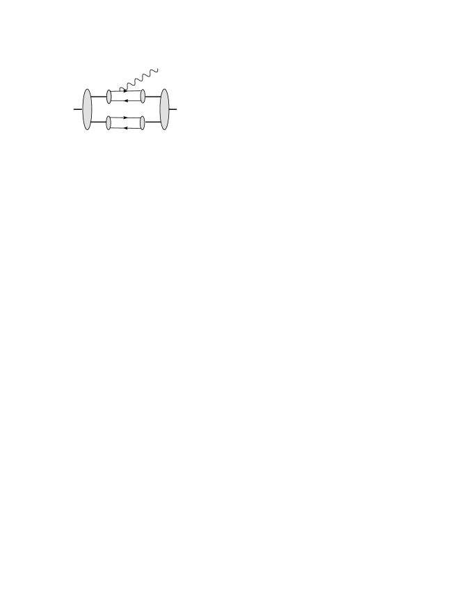
Figure 6: Molecule-Molecule Radiative Transition.

The resulting rate is given by

$$\Gamma_{MolMol} = {1\over 2}\Gamma(D^{*+}\to D^{+}\gamma;q_{*})F_{+}(q_{*})+$$ (25)

$${1\over 2}\Gamma(D^{*0}\to D^{0}\gamma;q_{*})F_{0}(q_{*})$$

where the width for $D^{*}\to D\gamma$ is evaluated at the photon momentum relevant to the $1^{+}\to\gamma 0^{+}$ process, $q_{*}$ This result has been obtained assuming that the momentum space wavefunction for the molecular state is strongly peaked at zero momentum, which will be the case for weakly bound states. The molecular form factors are given by

$$F_{\alpha}(q)=\int{d^{3}k\over(2\pi)^{3}}\psi^{(\alpha)}_{1^{+}}(k)\psi^{(\alpha)*}_{0^{+}}(k-{m_{K}\over m_{D}+m_{K}}q)$$ (26)

where the wavefunctions refer to the bound $D^{*}K$ and $DK$ systems respectively and $\alpha$ is a channel index denoting the $D^{(*)+}K^{0}$ or $D^{(*)0}K^{+}$ components of the molecules.

Weak binding implies that $q_{*}\approx m_{D^{*}}-m_{D}\approx 140$ MeV. This is reduced by the mass factor $m_{K}/(m_{D}+m_{K})=0.2$ in the argument of the wavefunction in Eq. 26. Thus the product is 28 MeV which is much smaller than the typical momenta in the weak binding potential, $\sqrt{2\mu_{DK}E_{B}}\approx 200$ MeV. Thus the form factor may be neglected and the predicted rate is given by the average of the neutral and charged M1 transitions, $D^{*}\to D\gamma$. Consulting Table 6 gives our final estimate $\Gamma(1^{+}(mol)\to 0^{+}(mol)\gamma)\approx 17$ keV, which may give a measurable branching ratio. This may be contrasted with the analogous $c\bar{s}$ transition predicted to be $(0.26\cos\phi_{s}+1.4\sin\phi_{s})^{2}\approx 1.0$ keV.

Measurement of the total widths of the $D_{s0}$ and $D_{s1}$ will be required before the emerging data can be compared with these predictionsDexpts .

IV.3 Radiative Transitions in the Heavy Quark Limit

As there are no charge conjugation constraints on the $D$ and $D_{s}$ systems, radiative transitions from ${}^{3}S_{1}$ can reach both ${}^{3}P_{J}$ and ${}^{1}P_{1}$ states. The most general transformation property of the transition at quark level is determined by noting that a positive helicity photon can change the projection of the spin or angular momentum of a quark by one unit. For radiative transitions between $S$ and $P$ levels the most general transformation for the current-quark operator is thus $AL_{+}+BS_{+}+CS_{z}L_{+}$, with unknown strengths $A,B,C$ (these can be calculated in specific models but here we wish to make more general conclusions). The relative amplitudes for transitions to the various $J^{P}$ states are then driven by Clebsch Gordan coefficients. The procedure is defined in Refs.cot and gives for the relative radiative amplitudes to or from $(0,1,2)^{+}$ :

$${\cal A}(V\to{}^{3}P_{0}\gamma) = {1\over\sqrt{3}}\left(A-C-{B\over\sqrt{2}}\right)$$ (27)

$${\cal A}(V\to 1_{L}\gamma)_{\lambda=0} = {1\over\sqrt{2}}\left((A-C)\sin\phi+B\cos\phi\right)$$ (28)

$${\cal A}(V\to 1_{L}\gamma)_{\lambda=1} = \left(A-\frac{B}{\sqrt{2}}\right){\sin\phi\over\sqrt{2}}+C\cos\phi$$ (29)

$${\cal A}(V\to{}^{3}P_{2}\gamma)_{\lambda=2} = A+C$$ (30)

$${\cal A}(V\to{}^{3}P_{2}\gamma)_{\lambda=1} = {1\over\sqrt{2}}\left(A+\frac{B}{\sqrt{2}}\right)$$ (31)

$${\cal A}(V\to{}^{3}P_{2}\gamma)_{\lambda=0} = {1\over\sqrt{6}}(A-C)+{1\over\sqrt{3}}B$$ (32)

Similar results hold for the decays involving the $1_{H}$.

These results simplify in the heavy quark limit, revealing some intriguing selection rules. In particular, in the heavy quark limit one has $\phi=-54.7^{o}$, which implies

$$-{\cal A}(V\to{}^{3}P_{0}\gamma) = {\cal A}(V\to 1_{L}\gamma)_{\lambda=0}$$ (33)

$$= {\cal A}(V\to 1_{L}\gamma)_{\lambda=1}$$

$${\cal A}(V\to 1_{H}\gamma)_{\lambda=0} = {\cal A}(V\to{}^{3}P_{2}\gamma)_{\lambda=0}$$ (34)

$${\cal A}(V\to 1_{H}\gamma)_{\lambda=1} = \sqrt{2\over 3}{\cal A}(V\to{}^{3}P_{2}\gamma)_{\lambda=2}-$$ (35)

$$\sqrt{1\over 3}{\cal A}(V\to{}^{3}P_{2}\gamma)_{\lambda=1}$$

The first of these corresponds to a selection rule which implies that the transition is pure $E1$ with $M2\equiv 0$ (this is immediately clear because the process ${}^{3}S_{1}\to{}^{3}P_{0}\gamma$ has no M2 amplitude). Hence the equality of amplitudes implies this is true for the $1_{L}$ rate as well. These relationships also imply that (apart from phase space corrections)

$$\Gamma(2^{3}S_{1}\to 1_{L}\gamma)=3\,\Gamma(2^{3}S_{1}\to{}^{3}P_{0}\gamma)$$ (36)

and

$$\Gamma(1_{L}\to{}^{3}S_{1}\gamma)=\Gamma({}^{3}P_{0}\to{}^{3}S_{1}\gamma).$$ (37)

Any deviation from these selection rules will measure deviations from the heavy quark limit and the heavy quark mixing angle.

The selection rules can be understood more immediately in the heavy quark $jj$ basis. Only the light flavoured constituent can change its quantum state in the limit $m_{Q}\to\infty$. In this case, the ${}^{3}S_{1}$ may be represented as $Q_{s(1/2)}\bar{q}_{s(1/2)}$ and the three independent $P$-states are combinations of $Q_{s(1/2)}$ and $\bar{q}$ in $p_{1/2}$ and $p_{3/2}$ with $j_{z}=\pm 1/2$ or $p_{3/2}$ with $j_{z}=\pm 3/2$. The three independent combinations of amplitudes in Eqs. 35 then correspond to the following: the transition $s_{1/2}\to p_{1/2}$ controls the identical amplitudes to the $0^{+}$ and $1^{+}(s_{1/2}p_{1/2})$ states; the transition $s_{1/2}\to p_{3/2}$ with $j_{z}=1/2$ determines the second relation; and the transition $s_{1/2}\to p_{3/2}$ with $j_{z}=3/2$ controls the third relationship.

With a large enough sample of $2^{3}S_{1}$ $c\bar{s}$ states, the radiative amplitudes to the $c\bar{s}$ $2^{+}$ and $1^{+}_{H}$ states can be compared with the selection rules to determine the mixing angle for the $1_{H}$ state in the ${}^{3}P_{1}-^{1}P_{1}$ basis. If the $1^{+}(2460)$ and $0^{+}(2317)$ are the remaining states in the $c\bar{s}$ $P$-wave system, the same mixing angle should emerge when extracted from radiative transitions involving this pair of states. If $O(10^{3})$ events are required to measure radiative amplitudes, and each of these states is produced with $b.r.(\sim 10^{-3})$, then approximately $10^{6}$ initial $2^{3}S_{1}$ mesons are required. Our estimates are that these arise at $\sim 10^{-2}$ in $B$ decays and so a suitable statistical sample should be accumulated at LHCb and other B-factories.

V Conclusions

Excited $D$ and $D_{s}$ states beyond the $P$-wave have not yet been identified. Moreover, mixing angles within the $P$ and $D$-waves are not yet quantified. Determining these observables is an important task for spectroscopy and heavy quark physics, and forms a vital prerequisite for electroweak and CP violation studies.

We expect that the emission of radially excited $D_{s}$ and $D_{s}^{*}$ will be significant in $B$-decays and can be anticipated at the 1% branching fraction level. Their decays give a potential source of $P$-wave $c\bar{s}$  states by which the ${}^{3}P-{}^{1}P$ mixing may be measured. This in turn can determine the $p_{3/2}-p_{1/2}$ mixing pattern, which is important in testing models of the enigmatic $D_{s}(2317)$ and $D_{s}(2460)$ states. For example chiral models implicitly assume that these are pure $p_{1/2}$ configurations while there need be no simple mixing pattern in $D^{(*)}K$ molecular interpretations. The $0^{+}$ and $1^{+}(p_{1/2})$ states will also be emitted in $B$-decays via the $W$ current. Their relative rates and the presence of one or two axial mesons in the data can also test the $p_{1/2}$ content and nature of the $D_{s}(2317)$ and $D_{s}(2460)$ states. Finally, radiative transitions also probe the quark structure of these hadrons and can assist in distinguishing molecular and $c\bar{s}$ assignments.

Two body decay modes of excited $D_{s}^{*}$ states have nodes in simple nonrelativistic models. Establishing the reality of these is important as such nodes have been invoked to explain anomalies in the $c\bar{c}$  spectrum above charm threshold. The presence of nodes could in principle cause states to have narrow widths, though we find this unlikely in the decays considered here unless unfavoured values of parameters are employed. In practice the nodes for certain decays tend to occur at energies where other channels have opened, thereby restoring a canonical width for the state. However, the nodes are still implicitly manifested by virtue of the ensuing anomalous branching ratios; for example, nodes might suppress the $DK$ channel while allowing a $D^{(**)}K^{(*)}$ decay, leading to relative rates that are an inversion of “phase space” expectations. Thus careful measurement of the relative branching ratios for $3^{3}S_{1}$ $D_{s}$ decays could prove to be a powerful tool for understanding gluodynamics in quark models.

Appendix A Decay Computation Details

A.1 Masses and SHO $\beta$ Values

The evaluation of the perturbative decay amplitudes requires mesonic wavefunctions. We follow tradition and employ SHO wavefunctions. Indeed, the model and experiment are sufficiently imprecise that computations with more realistic quark model reveal no systematic improvementsBG . The SHO wavefunction scale, denoted $\beta$ in the following, is typically taken as a parameter of the model. However, since we seek to describe the decay of heavy quark states, it is preferable to fix the SHO scales to quark model wavefunctions. This was achieved by choosing $\beta$ to reproduce the RMS radius of the quark model states. The resulting values are listed in Table 2.

Table 2: RMS Equivalent $\beta$ Values (GeV).

$n\,^{(2S+1)}L_{J}$	$uu$	$us$	$ss$	$uc$	$sc$	$cc$
$0\,^{1}S_{0}$	0.47 [0.4]	0.46 [0.4]	0.48	0.43	0.52	0.71
$0\,^{3}S_{1}$	0.28	0.32	0.36	0.37	0.45	0.66
$0\,^{3}P_{J}$	0.26	0.29	0.32	0.32	0.37	0.49
$0\,^{1}P_{1}$	0.27	0.29	0.33	0.33	0.38	0.50
$0\,^{3}D_{J}$	0.25	0.27	0.25	0.30	0.34	0.45
$0\,^{1}D_{2}$	0.25	0.27	0.25	0.30	0.35	0.45
$1\,^{1}S_{0}$	0.28	0.29	0.33	0.31	0.36	0.48
$1\,^{3}S_{1}$	0.24	0.26	0.30	0.30	0.35	0.47
$2\,^{1}S_{0}$	0.24	0.25	0.28	0.28	0.32	0.41
$2\,^{3}S_{1}$	0.23	0.24	0.27	0.27	0.31	0.41

The meson masses used to determine phase space and final state momenta are listed below.

Light meson masses:

$\pi=0.138$, $\eta=0.5477$, $\rho=0.7758$, $\omega=0.7826$, $K=0.495$, $K^{*}=0.8931$, $\eta^{\prime}=0.95778$.

$D$ meson masses:

$D=1.8694$, $D^{*}=2.0078$, $D_{1}=2.444$, $D_{1}^{\prime}=2.422$, $D_{2}=2.459$, $D_{0}=2.308$ (Belle), $D_{0}=2.407$ (Focus).

Two experimental values for the scalar $D$ meson mass are reported belle . Since these are incompatible we prefer to compute with both masses; leaving it to future experiment to choose between the options.

$D_{s}$ meson masses:

$D_{s}=1.9683$, $D_{s}^{*}=2.1121$, $D_{s0}=2.317$, $D_{s1}=2.459$, $D_{s1}^{\prime}=2.535$, $D_{s2}=2.572$.

Theoretical masses were:

$D^{\prime}=2.58$, ${D^{*}}^{\prime}=2.64$, $D^{\prime\prime}=3.25$, ${D^{*}}^{\prime\prime}=3.31$, $D(^{1}D_{2})=2.83$, $D(^{3}D_{1})=2.82$, $D(^{3}D_{2})=2.83$, $D(^{3}D_{3})=2.83$, $D_{s}^{\prime}=2.67$, ${D_{s}^{*}}^{\prime}=2.73$, $D_{s}^{\prime\prime}=3.24$, ${D_{s}^{*}}^{\prime\prime}=3.29$, $D_{s}(^{1}D_{2})=2.92$, $D_{s}(^{3}D_{1})=2.90$, $D_{s}(^{3}D_{2})=2.92$, $D_{s}(^{3}D_{3})=2.92$.

These were obtained from the quark model used to determine the SHO scale or from Ref. GI .

We set $D_{1}=D_{1}(2444)$ and $D_{1}^{\prime}=D_{1}(2422)$ since the latter is much narrower than the former. We also set $D_{s1}=D_{s1}(2459)$ and $D_{s1}^{\prime}=D_{s1}(2535)$ since both are narrow and the higher mass state is identified with the $D_{s1}^{\prime}$ in the heavy quark limit.

Finally, the quark model employed to determine the RMS $\beta$ values and the radiative transition rates is a standard color Coulomb plus linear scalar confinement interaction with the addition of a Gaussian-smeared contact hyperfine term. The central potential is thus

$$V(r)=\frac{4}{3}C-\frac{4}{3}\frac{\alpha_{s}}{r}+br+\frac{32\pi\alpha_{s}}{9m_{1}m_{2}}\,\tilde{\delta}_{\sigma}(r)\,\vec{\rm S}_{1}\cdot\vec{\rm S}_{2}\,$$ (38)

where $\tilde{\delta}_{\sigma}(r)=(\sigma/\sqrt{\pi})^{3}\,e^{-\sigma^{2}r^{2}}$. The parameters were chosen to reproduce a broad range of open flavour masses and are $C_{uc}=-346$ MeV, $C_{sc}=-319$ MeV, $b=0.162$ GeV², $\alpha=0.594$, and $\sigma=897$ MeV. Quark masses were taken to be $m_{u}=0.33$ GeV, $m_{s}=0.55$ GeV, and $m_{c}=1.6$ GeV in both radiative and strong computations.

A.2 Parameter Determination

A variety of ${}^{3}P_{0}$ models exist. These typically differ in the choice of weighting function used in the pair creation vertex, meson wavefunctions employed, and the phase space conventions. We shall restrict attention to the simplest vertex, which assumes a spatially uniform quark creation probability density. Possible phase space conventions include relativistic phase space (unit norm is used):

$${\rm(ps)}=2\pi k{E_{B}E_{C}\over m_{A}}$$ (39)

where $E_{B}$ is the energy of meson $B$ in the final state. This can differ substantially from the nonrelativistic version:

$${\rm(ps)}=2\pi k{m_{B}m_{C}\over(m_{B}+m_{C})}$$ (40)

especially when pions are in the final state. A third possibility, called the ‘mock meson’ method, is employed by Kokoski and IsgurKokoski:1985is :

$${\rm(ps)}=2\pi k{M_{B}M_{C}\over M_{A}}$$ (41)

where $M_{A}$ refers to the ‘mock meson’ mass of a state. This is defined to be the hyperfine-splitting averaged meson mass. In practice, the numerical result is little different from the relativistic phase space except for the case of the pion, where a mock mass of $M_{\pi}=0.77$ GeV is used. The final possibility is referred to as ’RPA phase space’PSS and postulates that the backward moving Fock components of pseudo-Goldstone bosons (pions and kaons) contribute to decays. In the chiral limit the net effect of this is to multiply amplitudes containing a single pion or kaon by a factor of 2; if two Goldstone bosons are present, the amplitude is multiplied by 3.

We have investigated the efficacy of six models in describing 32 well established experimental decay widths. These models all use SHO wavefunctions, either using a universal SHO width of $\beta=400$ MeV, the RMS-equivalent $\beta$ values of Table 2, or the RMS $\beta$s with the exception of $\beta_{\pi}$ and $\beta_{K}$ which are set to 400 MeV. The latter choice is an attempt to recognise that the lighter pseudoscalar states are Goldstone bosons and hence are likely to be larger than simple quark mode estimates. Relativistic and RPA phase space conventions have also been tested. We remark that the RPA and mock meson prescriptions yield similar results.

The resulting best fit ${}^{3}P_{0}$ couplings and their errors are listed in Table 3. As can be seen, the data and model are of sufficiently low quality that it is very difficult to distinguish the models (the models with $\beta_{\pi}=0.4$ obtain $\delta\gamma/\gamma\approx 38\%$ while employing $\beta_{RMS}$ yields $\delta\gamma/\gamma\approx 29\%$). We henceforth adopt the relativistic phase space convention with RMS $\beta$ values determined as in Table 2 and set $\gamma=0.485$.

Table 3: ${}^{3}P_{0}$ Couplings.

phase space	$\beta_{RMS}$	$\beta_{\pi}=0.4$	all $\beta=0.4$
Rel.	$0.485\pm 0.15$	$0.417\pm 0.16$	$0.505\pm 0.18$
RPA	$0.214\pm 0.06$	$0.186\pm 0.07$	$0.228\pm 0.09$

The couplings required to reproduce experiment in the 32 decay modes for the model used here are shown in Fig. 7. As can be seen, the large experimental errors preclude definitive conclusions. Nevertheless the model provides clear guidance over three orders of magnitude of predicted widths and over a broad range of quark flavours and meson quantum numbers. The specific decay modes are listed in Ref. modes

Figure 7: Equivalent Coupling vs. Mode. ${}^{3}P_{0}$ couplings required to reproduce experiment for 32 decay modes.

Appendix B E1 and M1 Radiative Transitions

Radiative transition rates based on Eq. 19 and the mixed states of Section II.2 are reported here.

Table 4: E1 Radiative Transitions in the $D$ System

mode	q (MeV)	$\Gamma$ (keV)
$D_{2}^{+}\to D^{*+}\gamma$	408	51
$D_{2}^{0}\to D^{*0}\gamma$	410	895
$D_{0}^{+}\to D^{*+}\gamma$	$\pmatrix{279\\ 364}$	$\pmatrix{17\\ 37}$
$D_{0}^{0}\to D^{*0}\gamma$	$\pmatrix{281\\ 367}$	$\pmatrix{304\\ 649}$
${D^{*}}{{}^{\prime+}}\to D_{0}^{+}\gamma$	$\pmatrix{311\\ 223}$	$\pmatrix{10.0\\ 3.8}$
${D^{*}}{{}^{\prime 0}}\to D_{0}^{0}\gamma$	$\pmatrix{311\\ 223}$	$\pmatrix{173\\ 66}$
${D^{*}}{{}^{\prime+}}\to D_{2}^{+}\gamma$	175	9.4
${D^{*}}{{}^{\prime 0}}\to D_{2}^{0}\gamma$	175	163
$D_{1}^{+}\to D^{*+}\gamma$	377	$s^{2}$ 41
$D_{1}^{0}\to D^{*0}\gamma$	379	$s^{2}$ 715
${D_{1}^{\prime}}^{+}\to D^{*+}\gamma$	395	$c^{2}$ 46
${D_{1}^{\prime}}^{0}\to D^{*0}\gamma$	398	$c^{2}$ 819
${D^{*}}^{\prime+}\to D_{1}^{+}\gamma$	209	$s^{2}$ 9.5
${D^{*}}^{\prime 0}\to D_{1}^{0}\gamma$	209	$s^{2}$ 164
${D^{*}}^{\prime+}\to{D_{1}}^{\prime+}\gamma$	189	$c^{2}$ 7.0
${D^{*}}^{\prime 0}\to{D_{1}}^{\prime 0}\gamma$	189	$c^{2}$ 122
$D_{1}^{+}\to D^{+}\gamma$	490	$c^{2}$ 59
$D_{1}^{0}\to D^{0}\gamma$	493	$c^{2}$ 1046
${D_{1}}^{\prime+}\to D^{+}\gamma$	507	$s^{2}$ 66
${D_{1}}^{\prime 0}\to D^{0}\gamma$	510	$s^{2}$ 1154
${D}^{\prime+}\to D_{1}^{+}\gamma$	153	$c^{2}$ 14
${D}^{\prime 0}\to D_{1}^{0}\gamma$	153	$c^{2}$ 233
${D}^{\prime+}\to{D_{1}}^{\prime+}\gamma$	132	$s^{2}$ 8.8
${D}^{\prime 0}\to{D_{1}}^{\prime 0}\gamma$	132	$s^{2}$ 152

Table 5: E1 Radiative Transitions in the $D_{s}$ System

mode	q (MeV)	$\Gamma$ (keV)
$D_{s2}\to D_{s}^{*}\gamma$	419	8.8
$D_{s0}\to D_{s}^{*}\gamma$	196	1.0
${D_{s}^{*}}^{\prime}\to D_{s0}\gamma$	382	3.3
${D_{s}^{*}}^{\prime}\to D_{s2}\gamma$	153	1.2
$D_{s1}\to D_{s}^{*}\gamma$	323	$s^{2}$ 4.2
${D_{s1}}^{\prime}\to D_{s}^{*}\gamma$	388	$c^{2}$ 7.1
$D_{s1}\to D_{s}\gamma$	442	$c^{2}$ 7.3
${D_{s1}}^{\prime}\to D_{s}\gamma$	504	$s^{2}$ 10.6
${D_{s}^{*}}^{\prime}\to D_{s1}\gamma$	258	$s^{2}$ 3.2
${D_{s}^{*}}^{\prime}\to D_{s1}^{\prime}\gamma$	188	$c^{2}$ 1.3
$D_{s}^{\prime}\to D_{s1}\gamma$	203	$c^{2}$ 5.4
$D_{s}^{\prime}\to D_{s1}^{\prime}\gamma$	132	$s^{2}$ 1.5

Table 6: M1 Radiative Transitions

mode	q (MeV)	$\Gamma$ (keV)	$\Gamma$ (keV) PDG
$D^{*+}\to D^{+}\gamma$	136	1.8	$1.5\pm 0.5$
$D^{*0}\to D^{0}\gamma$	137	32	$<800$
$D_{1}^{+}\to D_{0}^{+}\gamma$	$\pmatrix{132\\ 37}$	$\pmatrix{(0.7c+1.8s)^{2}\\ (0.11c+0.28s)^{2}}$
$D_{1}^{0}\to D_{0}^{0}\gamma$	$\pmatrix{132\\ 37}$	$\pmatrix{(3.2c+2.0s)^{2}\\ (0.47c+0.31s)^{2}}$
${D_{1}^{+}}^{\prime}\to D_{0}^{+}\gamma$	$\pmatrix{111\\ 15}$	$\pmatrix{(-0.56s+1.4c)^{2}\\ (-0.031s+0.07c)^{2}}$
${D_{1}^{0}}^{\prime}\to D_{0}^{0}\gamma$	$\pmatrix{111\\ 15}$	$\pmatrix{(-2.4s+1.6c0^{2}\\ (-0.12s+0.08c)^{2}}$
$D_{s}^{*}\to D_{s}\gamma$	139	0.2
$D_{s1}\to D_{s0}\gamma$	139	$(0.26c+1.4s)^{2}$
$D_{s1}^{\prime}\to D_{s0}\gamma$	209	$(-0.44s+2.5c)^{2}$

Appendix C Tables of Open Flavour Strong Decay Modes

Strong decay rates and amplitudes are collected in Tables 7 to 14. In the following $c$ and $s$ refer to $P$-wave mixing in the $D$ or $D_{s}$ sector $c=\cos\phi$ or $\cos\phi_{s}$. Mixing angles in the $D$-waves are labelled $c_{1}$ or $s_{1}$; thus $c_{1}=\cos\phi_{D}$ or $\cos\phi_{Ds}$. Estimates of decay rates containing mixing angles are given in terms of the theoretical heavy quark predictions. Rates for modes containing the Belle and Focus $D_{0}$ are presented separately; when both may occur the differing possible total widths are separated by a slash.

Table 7: Open-flavor strong decays

State	Mode	$\Gamma_{thy}$   [$\Gamma_{expt}$] (MeV)	Amps. (GeV-1/2)
$\rm D^{*+}$	$\rm D^{0}\pi^{+}$	25 keV [64(15) keV]	${}^{1}P_{1}=-0.027$
$\rm D^{*+}$	$\rm D^{+}\pi^{0}$	11 keV [29(6.8) keV]	${}^{1}P_{1}=-0.019$
$\rm D^{*0}$	$\rm D^{0}\pi^{0}$	16 keV [$<$ 2.1 MeV]	${}^{1}P_{1}=-0.021$
$\rm D_{0}(2308)$	$\rm D\pi$	316 [276(66)]	${}^{1}S_{0}=+0.635$
$\rm D_{0}(2407)$	$\rm D\pi$	283 [276(66)]	${}^{1}S_{0}=+0.504$
$\rm D_{1}$	$\rm D^{*}\pi$	$110c^{2}+191s^{2}-230sc=272$ [329(84)]	${}^{3}S_{1}=-0.338c+0.478s$, ${}^{3}D_{1}=-0.153c-0.108s$
$\rm D_{1}^{\prime}$	$\rm D^{*}\pi$	$191c^{2}+106s^{2}+240sc=22$ [19(5)]	${}^{3}S_{1}=+0.504c+0.357s$, ${}^{3}D_{1}=-0.099c+0.141s$
$\rm D_{2}$	$\rm D\pi$	35	${}^{1}D_{2}=+0.164$
	$\rm D^{*}\pi$	20	${}^{3}D_{2}=-0.154$
	$\rm D\eta$	0.08	${}^{1}D_{2}=+0.013$
	total:	55 [24(5)]

Table 8: Open-flavor strong decays, continued

State	Mode	$\Gamma_{thy}$   [$\Gamma_{expt}$] (MeV)	Amps. (GeV-1/2)
$\rm D^{\prime}$	$\rm D^{*}\pi$	27	${}^{3}P_{0}=-0.145$
	$\rm D_{0}(2308)\pi$	41	${}^{1}S_{0}=+0.355$
	$\rm D_{0}(2407)\pi$	18	${}^{1}S_{0}=+0.416$
	$\rm D^{*}\eta$	1	${}^{3}P_{0}=-0.051$
	total:	69/46
$\rm D^{*^{\prime}}$	$\rm D\pi$	1	${}^{1}P_{1}=-0.025$
	$\rm D^{*}\pi$	5	${}^{3}P_{1}=-0.059$
	$\rm D\eta$	0.4	${}^{1}P_{1}=+0.016$
	$\rm D_{s}K$	0.1	${}^{1}P_{1}=+0.010$
	$\rm D^{*}\eta$	2	${}^{3}P_{1}=-0.055$
	$\rm D_{1}\pi$	$11c^{2}+22s^{2}-31sc=33$	${}^{3}S_{1}=-0.270c+0.381s$
			${}^{3}D_{1}=-0.034c-0.024s$
	$\rm D_{1}^{\prime}\pi$	$27c^{2}+14s^{2}+38sc=1$	${}^{3}S_{1}=+0.369c+0.261s$
			${}^{3}D_{1}=-0.035c+0.049s$
	$\rm D_{2}\pi$	0.1	${}^{5}D_{1}=+0.031$
	$\rm D_{s}^{*}K$	0.7	${}^{3}P_{1}=-0.041$
	total:	44

Table 9: Open-flavor strong decays, continued

State	Mode	$\Gamma_{thy}$   [$\Gamma_{expt}$] (MeV)	Amps. (GeV-1/2)
$\rm D(^{3}D_{1})$	$\rm D\pi$	73	${}^{1}P_{1}=-0.161$
	$\rm D^{*}\pi$	45	${}^{3}P_{1}=-0.141$
	$\rm D\eta$	16	${}^{1}P_{1}=-0.082$
	$\rm D_{s}K$	55	${}^{1}P_{1}=-0.164$
	$\rm D^{*}\eta$	9	${}^{3}P_{1}=-0.071$
	$\rm D_{1}\pi$	$131c^{2}+64s^{2}+183sc=0.2$	${}^{3}S_{1}=+0.442c+0.312s$
			${}^{3}D_{1}=+0.106c+0.051s$
	$\rm D_{1}^{\prime}\pi$	$61c^{2}+127s^{2}-176sc=189$	${}^{3}S_{1}=+0.288c-0.409s$
			${}^{3}D_{1}=+0.057c-0.115s$
	$\rm D_{2}\pi$	7	${}^{5}D_{1}=+0.108$
	$\rm D_{s}^{*}K$	23	${}^{3}P_{1}=-0.129$
	$\rm D\rho$	74	${}^{3}P_{1}=-0.207$
	$\rm D\omega$	16	${}^{3}P_{1}=-0.098$
	$\rm D^{*}\rho$	13	${}^{1}P_{1}=-0.117$, ${}^{3}P_{1}=0$, ${}^{5}P_{1}=0.052$, ${}^{5}F_{1}=0.025$
	$\rm D^{*}\omega$	3	${}^{1}P_{1}=-0.063$, ${}^{3}P_{1}=0$, ${}^{5}P_{1}=0.028$, ${}^{5}F_{1}=0.011$
	total:	523
$\rm D(^{3}D_{3})$	$\rm D\pi$	53	${}^{1}F_{3}=-0.136$
	$\rm D^{*}\pi$	55	${}^{3}F_{3}=+0.155$
	$\rm D\eta$	4	${}^{1}F_{3}=-0.041$
	$\rm D_{s}K$	4	${}^{1}F_{3}=-0.044$
	$\rm D^{*}\eta$	3	${}^{3}F_{3}=+0.037$
	$\rm D_{1}\pi$	$3.5c^{2}+0.5s^{2}-2.3sc=3$	${}^{3}D_{3}=+0.071c-0.026s$
			${}^{3}G_{3}=+0.013c+0.009s$
	$\rm D_{1}^{\prime}\pi$	$0.6c^{2}+4.6s^{2}+2.8sc=2$	${}^{3}D_{3}=-0.027c-0.077s$
			${}^{3}G_{3}=+0.011c-0.016s$
	$\rm D_{2}\pi$	6	${}^{5}D_{3}=-0.099$, ${}^{5}G_{3}=-0.010$
	$\rm D_{s}^{*}K$	2	${}^{3}F_{3}=+0.034$
	$\rm D\rho$	15	${}^{3}F_{3}=+0.090$
	$\rm D\omega$	4	${}^{3}F_{3}=+0.050$
	$\rm D^{*}\rho$	99	${}^{5}P_{3}=-0.009$, ${}^{1}F_{3}=0.343$, ${}^{3}F_{3}=0$, ${}^{5}H_{3}=0.019$
	$\rm D^{*}\omega$	27	${}^{5}P_{3}=-0.004$, ${}^{1}F_{3}=0.188$, ${}^{3}F_{3}=0$, ${}^{5}H_{3}=0.009$
	$\rm D\eta^{\prime}$	$\approx 0$	${}^{1}F_{3}=-5.5\cdot 10^{-5}$
	total:	277

Table 10: Open-flavor strong decays, continued

State	Mode	$\Gamma_{thy}$   [$\Gamma_{expt}$] (MeV)	Amps. (GeV-1/2)
${\rm D_{2}^{*}}$	$\rm D^{*}\pi$	$93c_{1}^{2}+91s_{1}^{2}+9s_{1}c_{1}=87$	${}^{3}P_{2}=+0.123c_{1}-0.151s_{1}$
			${}^{3}F_{2}=+0.158c_{1}+0.129s_{1}$
	$\rm D_{0}(2308)\pi$	$0.8c_{1}^{2}+1.9s_{1}^{2}+2.4s_{1}c_{1}=0.4$	${}^{1}D_{2}=-0.026c_{1}-0.041s_{1}$
	$\rm D_{0}(2407)\pi$	$0.9c_{1}^{2}+0.7s_{1}^{2}+1.6s_{1}c_{1}=0.02$	${}^{1}D_{2}=-0.034c_{1}-0.031s_{1}$
	$\rm D^{*}\eta$	$13c_{1}^{2}+18s_{1}^{2}-22s_{1}c_{1}=27$	${}^{3}P_{2}=+0.077c_{1}-0.094s_{1}$
			${}^{3}F_{2}=+0.038c_{1}+0.032s_{1}$
	$\rm D_{1}\pi$	$0.7c_{1}^{2}s^{2}+5.1s_{1}^{2}c^{2}+7.6s_{1}^{2}s^{2}+$	${}^{3}D_{2}=-0.032c_{1}s-0.087s_{1}c-0.107s_{1}s$
		$3.8c_{1}s_{1}sc+4.6c_{1}s_{1}s^{2}+12.5s_{1}^{2}sc=0.1$
	$\rm D_{1}^{\prime}\pi$	$0.9c_{1}^{2}c^{2}+9.8s_{1}^{2}c^{2}+6.8s_{1}^{2}s^{2}+$	${}^{3}D_{2}=-0.035c_{1}c+0.096s_{1}s-0.115s_{1}c$
		$6.0c_{1}s_{1}c^{2}-5.0c_{1}s_{1}sc-16.3s_{1}^{2}sc=8.4$
	$\rm D_{2}\pi$	$86c_{1}^{2}+115s_{1}^{2}-195s_{1}c_{1}=197$	${}^{5}S_{2}=-0.349c_{1}+0.427s_{1}$
			${}^{5}D_{2}=-0.130c_{1}+0.067s_{1}$
			${}^{5}G_{2}=-0.013c_{1}-0.011s_{1}$
	$\rm D_{s}^{*}K$	$31c_{1}^{2}+45s_{1}^{2}-69s_{1}c_{1}=73$	${}^{3}P_{2}=+0.142c_{1}-0.174s_{1}$
			${}^{3}F_{2}=+0.035c_{1}+0.029s_{1}$
	$\rm D\rho$	$75c_{1}^{2}+100s_{1}^{2}-122s_{1}c_{1}=150$	${}^{3}P_{2}=+0.183c_{1}-0.224s_{1}$
			${}^{3}F_{2}=+0.092c_{1}+0.075s_{1}$
	$\rm D\omega$	$25c_{1}^{2}+33s_{1}^{2}-41s_{1}c_{1}=50$	${}^{3}P_{2}=+0.106c_{1}-0.130s_{1}$
			${}^{3}F_{2}=+0.051c_{1}+0.042s_{1}$
	$\rm D^{*}\rho$	$50c_{1}^{2}+25s_{1}^{2}=33$	${}^{3}D_{2}=-0.243c_{1}$, ${}^{5}D_{2}=0.172s_{1}$
			${}^{3}F_{2}=-0.025c_{1}$, ${}^{5}F_{2}=0.029s_{1}$
	$\rm D^{*}\omega$	$14c_{1}^{2}+7s_{1}^{2}=9$	${}^{3}D_{2}=-0.133c_{1}$, ${}^{5}D_{2}=0.094s_{1}$
			${}^{3}F_{2}=-0.012c_{1}$, ${}^{5}F_{2}=0.014s_{1}$
	$\rm D_{s0}K$	$\approx 0$	${}^{1}D_{2}=-0.007c_{1}-0.003s_{1}$
	total:	$389c_{1}^{2}+437s_{1}^{2}-409s_{1}c_{1}$ + 8
${\rm D_{2}^{*}}^{\prime}$	$\rm D^{*}\pi$	$91c_{1}^{2}+93s_{1}^{2}-9s_{1}c_{1}=96$	${}^{3}D_{2}=-0.151c_{1}-0.123s_{1}$
			${}^{3}F_{2}=+0.129c_{1}-0.158s_{1}$
	$\rm D_{0}(2308)\pi$	$1.9c_{1}^{2}+0.8s_{1}^{2}-2.4s_{1}c_{1}=2.3$	${}^{1}D_{2}=-0.041c_{1}+0.026s_{1}$
	$\rm D_{0}(2407)\pi$	$0.7c_{1}^{2}+0.9s_{1}^{2}-1.6s_{1}c_{1}=1.6$	${}^{1}D_{2}=-0.031c_{1}-0.034s_{1}$
	$\rm D^{*}\eta$	$18c_{1}^{2}+13s_{1}^{2}+22s_{1}c_{1}=4.5$	${}^{3}D_{2}=-0.094c_{1}-0.077s_{1}$
			${}^{3}F_{2}=+0.031c_{1}-0.038s_{1}$
	$\rm D_{1}\pi$	$5.1c_{1}^{2}c^{2}+7.6c^{2}s^{2}+0.7s_{1}^{2}s^{2}+$	${}^{3}D_{2}=+0.032s_{1}s-0.087c_{1}c-0.106c_{1}s$
		$12.5c_{1}^{2}cs-3.8c_{1}s_{1}cs-4.6c_{1}s_{1}s^{2}=1.2$
	$\rm D_{1}^{\prime}\pi$	$9.8c_{1}^{2}c^{2}+6.8c_{1}^{2}s^{2}+0.9s_{1}^{2}c^{2}-$	${}^{3}D_{2}=+0.035s_{1}c+0.096c_{1}s-0.115c_{1}c$
		$-16c_{1}^{2}sc-6.0c_{1}s_{1}c^{2}+5.0c_{1}s_{1}sc=7.5$
	$\rm D_{2}\pi$	$115c_{1}^{2}+86s_{1}^{2}+195s_{1}c_{1}=3.9$	${}^{5}S_{2}=+0.427c_{1}+0.349s_{1}$
			${}^{5}D_{2}=+0.067c_{1}+0.131s_{1}$
			${}^{5}G_{2}=-0.011c_{1}+0.013s_{1}$
	$\rm D_{s}^{*}K$	$45c_{1}^{2}+31s_{1}^{2}+69s_{1}c_{1}=3.3$	${}^{3}D_{2}=-0.174c_{1}-0.142s_{1}$
			${}^{3}F_{2}=0.086c_{1}-0.035s_{1}$
	$\rm D\rho$	$100c_{1}^{2}+75s_{1}^{2}+122s_{1}c_{1}=26$	${}^{3}D_{2}=-0.224c_{1}-0.183s_{1}$
			${}^{3}F_{2}=+0.075c_{1}-0.092s_{1}$
	$\rm D\omega$	$33c_{1}^{2}+25s_{1}^{2}+41s_{1}c_{1}=7.9$	${}^{3}D_{2}=-0.130c_{1}-0.106s_{1}$
			${}^{3}F_{2}=+0.042c_{1}-0.051s_{1}$
	$\rm D^{*}\rho$	$25c_{1}^{2}+50s_{1}^{2}=42$	${}^{3}D_{2}=+0.243s_{1}$, ${}^{5}D_{2}=0.172c_{1}$
			${}^{3}F_{2}=-0.025s_{1}$, ${}^{5}F_{2}=0.029c_{1}$
	$\rm D^{*}\omega$	$7c_{1}^{2}+14s_{1}^{2}=12$	${}^{3}D_{2}=+0.133s_{1}$, ${}^{5}D_{2}=0.094c_{1}$
			${}^{3}F_{2}=+0.012s_{1}$, ${}^{5}F_{2}=0.014c_{1}$
	$\rm D_{s0}K$	$\approx 0$	${}^{1}D_{2}=-0.003c_{1}+0.007s_{1}$
	total:	$437c_{1}^{2}+389s_{1}^{2}+409s_{1}c_{1}+9$

Table 11: Open-flavor strong decays, continued

State	Mode	$\Gamma_{thy}$   [$\Gamma_{expt}$] (MeV)	Amps. (GeV-1/2)
$\rm D^{\prime\prime}(3.23)$	$\rm D^{*}\pi$	46	${}^{3}P_{0}=+0.103$
	$\rm D_{0}(2308)\pi$	72	${}^{1}S_{0}=+0.154$
	$\rm D_{0}(2407)\pi$	63	${}^{1}S_{0}=+0.156$
	$\rm D^{*}\eta$	1.6	${}^{3}P_{0}=+0.020$
	$\rm D_{2}\pi$	36	${}^{5}D_{0}=+0.124$
	$\rm D_{s}^{*}K$	1.8	${}^{3}P_{0}=+0.022$
	$\rm D\rho$	1.4	${}^{3}P_{0}=-0.018$
	$\rm D\omega$	0.6	${}^{3}P_{0}=-0.012$
	$\rm D^{*}\rho$	39	${}^{3}P_{0}=+0.105$
	$\rm D^{*}\omega$	13	${}^{3}P_{0}=+0.061$
	$\rm D_{s0}K$	47	${}^{1}S_{0}=+0.134$
	$\rm D_{0}(2308)\eta$	11	${}^{1}S_{0}=+0.066$
	$\rm D_{s}K^{*}$	2.2	${}^{3}P_{0}=-0.026$
	$\rm D_{s}^{*}K^{*}$	3	${}^{3}P_{0}=+0.034$
	$\rm D_{2}\eta$	$\approx 0$	${}^{5}D_{0}=-0.004$
	total:	275/266
$\rm D^{*^{\prime\prime}}(3.31)$	$\rm D\pi$	53	${}^{1}P_{1}=-0.100$
	$\rm D^{*}\pi$	59	${}^{3}P_{1}=+0.112$
	$\rm D\eta$	5	${}^{1}P_{1}=-0.033$
	$\rm D_{s}K$	14	${}^{1}P_{1}=-0.055$
	$\rm D^{*}\eta$	4	${}^{3}P_{1}=+0.030$
	$\rm D_{1}\pi$	$50c^{2}+62s^{2}-34sc=74$	${}^{3}S_{1}=-0.095c+0.135s$
			${}^{3}D_{1}=-0.096c-0.068s$
	$\rm D_{1}^{\prime}\pi$	$65c^{2}+53s^{2}+33sc=42$	${}^{3}S_{1}=+0.134c+0.095s$
			${}^{3}D_{1}=-0.070c+0.099s$
	$\rm D_{2}\pi$	35	${}^{5}D_{1}=+0.115$
	$\rm D_{s}^{*}K$	7	${}^{3}P_{1}=+0.041$
	$\rm D\rho$	3	${}^{3}P_{1}=+0.024$
	$\rm D\omega$	1	${}^{3}P_{1}=+0.013$
	$\rm D^{*}\rho$	12	${}^{1}P_{1}=+0.012$, ${}^{3}P_{1}=0$, ${}^{5}P_{1}=-0.055$, ${}^{5}F_{1}=0$
	$\rm D^{*}\omega$	5	${}^{1}P_{1}=+0.007$, ${}^{3}P_{1}=0$, ${}^{5}P_{1}=-0.034$, ${}^{5}F_{1}=0$
	$\rm D\eta^{\prime}$	0.5	${}^{1}P_{1}=-0.011$
	$\rm D_{s}K^{*}$	0.7	${}^{3}P_{1}=-0.013$
	$\rm D_{s1}K$	$20c^{2}+34s^{2}-41sc=49$	${}^{3}S_{1}=-0.085c+0.120s$
			${}^{3}D_{1}=-0.039c-0.028s$
	$\rm D_{s1}^{\prime}K$	$27c^{2}+14s^{2}+36sc=2$	${}^{3}S_{1}=+0.120c+0.085s$
			${}^{3}D_{1}=-0.017c+0.024s$
	$\rm D_{1}\eta$	$4.3c^{2}+7.9s^{2}-9.8sc=11$	${}^{3}S_{1}=-0.041c+0.058s$
			${}^{3}D_{1}=-0.016c-0.012s$
	$\rm D_{1}^{\prime}\eta$	$8.3c^{2}+4.9s^{2}+9.8sc=1$	${}^{3}S_{1}=+0.058c+0.041s$
			${}^{3}D_{1}=-0.014c+0.020s$
	$\rm D_{s}^{*}K^{*}$	7	${}^{1}P_{1}=+0.011$, ${}^{3}P_{1}=0$, ${}^{5}P_{1}=-0.047$, ${}^{5}F_{1}=0$
	$\rm D_{2}\eta$	0.6	${}^{1}P_{1}=+0.017$
	$\rm D_{0}(2308)\rho$	10	${}^{3}S_{1}=+0.066$, ${}^{3}D_{1}=0$
	$\rm D_{0}(2308)\omega$	3	${}^{3}S_{1}=+0.038$, ${}^{3}D_{1}=0$
	$\rm D_{s0}K^{*}$	0.3	${}^{3}S_{1}=+0.013$, ${}^{3}D_{1}=0$
	total:	399/386

Table 12: Open-flavor strong decays, continued

State	Mode	$\Gamma_{thy}$   [$\Gamma_{expt}$] (MeV)	Amps. (GeV-1/2)
$\rm D_{s1}^{\prime}$	$\rm D^{*}K$	$261c^{2}+131s^{2}-369sc=0.8$ [$<$ 2.3]	${}^{3}S_{1}=0.789c+0.557s$, ${}^{3}D_{1}=-0.024c+0.035s$
$\rm D_{s2}$	$\rm DK$	27	${}^{1}D_{2}=+0.143$
	$\rm D^{*}K$	3.1	${}^{3}D_{2}=-0.069$
	$\rm D_{s}\eta$	0.2	${}^{1}D_{2}=-0.018$
	total:	30 [15(5)]
$\rm D_{s}^{\prime}$	$\rm D^{*}K$	126	${}^{3}P_{0}=-0.330$
	$\rm D_{s}^{*}\eta$	0.5	${}^{3}P_{0}=+0.043$
	total:	127
$\rm D_{s}^{*^{\prime}}$	$\rm DK$	17	${}^{1}P_{1}=+0.090$
	$\rm D^{*}K$	81	${}^{3}P_{1}=-0.236$
	$\rm D_{s}\eta$	2.6	${}^{1}P_{1}=-0.042$
	$\rm D_{s}^{*}\eta$	4.1	${}^{3}P_{1}=+0.074$
	total:	105

Table 13: Open-flavor strong decays, continued

State	Mode	$\Gamma_{thy}$   [$\Gamma_{expt}$] (MeV)	Amps. (GeV-1/2)
$\rm D_{s}(^{3}D_{1})$	$\rm DK$	120	${}^{1}P_{1}=-0.205$
	$\rm D^{*}K$	74	${}^{3}P_{1}=-0.181$
	$\rm D_{s}\eta$	39	${}^{1}P_{1}=+0.129$
	$\rm D_{s}^{*}\eta$	17	${}^{3}P_{1}=+0.102$
	$\rm DK^{*}$	81	${}^{3}P_{1}=-0.218$
	total:	331
$\rm D_{s2}^{*}$	$\rm D^{*}K$	$155c_{1}^{2}+174s_{1}^{2}-92s_{1}c_{1}=211$	${}^{3}P_{2}=+0.189c_{1}-0.232s_{1}$
			${}^{3}F_{2}=+0.173c_{1}+0.141s_{1}$
	$\rm D_{s}^{*}\eta$	$24c_{1}^{2}+35s_{1}^{2}-51s_{1}c_{1}=55$	${}^{3}P_{2}=-0.112c_{1}+0.137s_{1}$
			${}^{3}F_{2}=-0.036c_{1}-0.029s_{1}$
	$\rm DK^{*}$	$118c_{1}^{2}+165s_{1}^{2}-230s_{1}c_{1}=258$	${}^{3}P_{2}=+0.237c_{1}-0.290s_{1}$
			${}^{3}F_{2}=+0.089c_{1}+0.073s_{1}$
	$\rm D_{0}(2308)K$	$0.04c_{1}^{2}+0.78s_{1}^{2}+0.34s_{1}c_{1}=0.4$	${}^{1}D_{2}=-0.006c_{1}-0.029s_{1}$
	$\rm D_{s0}\eta$	$0.07c_{1}^{2}+0.04s_{1}^{2}+0.11s_{1}c_{1}\approx 0$	${}^{1}D_{2}=+0.010c_{1}+0.008s_{1}$
	$\rm D^{*}K^{*}$	$26c_{1}^{2}+13s_{1}^{2}=17$	${}^{3}P_{2}=-0.207c_{1}$, ${}^{5}P_{2}=0.147s_{1}$
			${}^{3}F_{2}=-0.008c_{1}$, ${}^{5}F_{2}=0.009s_{1}$
	$\rm D_{0}(2407)K$	$\approx 0$	${}^{1}D_{2}=-0.003c_{1}-0.0055s_{1}$
	$\rm D_{1}^{\prime}K$	$\approx 0$	${}^{3}D_{2}=-0.0009c_{1}c+0.0026s_{1}s-0.0026s_{1}c$
	total:	$323c_{1}^{2}+389s_{1}^{2}-373s_{1}c_{1}$
${\rm D_{s2}^{*}}^{\prime}$	$\rm D^{*}K$	$174c_{1}^{2}+155s_{1}^{2}+92s_{1}c_{1}=118$	${}^{3}P_{2}=-0.232c_{1}-0.189s_{1}$
			${}^{3}F_{2}=+0.141c_{1}-0.173s_{1}$
	$\rm D_{s}^{*}\eta$	$35c_{1}^{2}+24s_{1}^{2}+51s_{1}c_{1}=4.0$	${}^{3}P_{2}=+0.137c_{1}+0.112s_{1}$
			${}^{3}F_{2}=-0.029c_{1}+0.036s_{1}$
	$\rm DK^{*}$	$165c_{1}^{2}+118s_{1}^{2}+230s_{1}c_{1}=25$	${}^{3}P_{2}=-0.290c_{1}-0.237s_{1}$
			${}^{3}F_{2}=+0.073c_{1}-0.089s_{1}$
	$\rm D_{0}(2308)K$	$0.78c_{1}^{2}+0.04s_{1}^{2}-0.34s_{1}c_{1}=0.4$	${}^{1}D_{2}=-0.028c_{1}-0.0006s_{1}$
	$\rm D_{s0}\eta$	$\approx 0$	${}^{1}D_{2}=+0.008c_{1}-0.010s_{1}$
	$\rm D^{*}K^{*}$	$13c_{1}^{2}+26s_{1}^{2}=17$	${}^{3}P_{2}=-0.207s_{1}$, ${}^{5}P_{2}=0.145c_{1}$
			${}^{3}F_{2}=+0.008s_{1}$, ${}^{5}F_{2}=0.009c_{1}$
	$\rm D_{0}(2407)K$	$\approx 0$	${}^{1}D_{2}=-0.005c_{1}+0.003s_{1}$
	$\rm D_{1}^{\prime}K$	$\approx 0$	${}^{3}D_{2}=-0.0009s_{1}c+0.003c_{1}s-0.003c_{1}c$
	total:	$389c_{1}^{2}+323s_{1}^{2}+373s_{1}c_{1}$
$\rm D_{s}(^{3}D_{3})$	$\rm DK$	82	${}^{1}F_{3}=-0.166$
	$\rm D^{*}K$	67	${}^{3}F_{3}=+0.168$
	$\rm D_{s}\eta$	4.5	${}^{1}F_{3}=+0.043$
	$\rm D_{s}^{*}\eta$	2.2	${}^{3}F_{3}=-0.035$
	$\rm DK^{*}$	14	${}^{3}F_{3}=+0.087$
	$\rm D^{*}K^{*}$	52	${}^{5}P_{3}=-0.003$, ${}^{1}F_{3}=0.294$, ${}^{3}F_{3}=0$, ${}^{5}F_{3}=0.006$, ${}^{5}H_{3}=0$
	$\rm D_{1}^{\prime}K$	$\approx 0$	${}^{3}D_{3}=-0.0004c-0.0017s$, ${}^{3}G_{3}\approx 0$
	total:	222

Table 14: Open-flavor strong decays, continued

State	Mode	$\Gamma_{thy}$   [$\Gamma_{expt}$] (MeV)	Amps. (GeV-1/2)
$\rm D_{s}^{\prime\prime}(3.23)$	$\rm D^{*}K$	3.5	${}^{3}P_{0}=-0.030$
	$\rm D_{s}^{*}\eta$	1.9	${}^{3}P_{0}=+0.024$
	$\rm DK^{*}$	39	${}^{3}P_{0}=-0.100$
	$\rm D_{0}(2308)K$	47	${}^{1}S_{0}=+0.134$
	$\rm D_{s0}\eta$	13	${}^{1}S_{0}=-0.073$
	$\rm D^{*}K^{*}$	72	${}^{3}P_{0}=+0.152$
	$\rm D_{0}(2407)K$	35	${}^{1}S_{0}=+0.129$
	$\rm D_{2}K$	43	${}^{5}D_{0}=-0.151$
	total:	219/207
${\rm D_{s}^{*}}^{\prime\prime}(3.29)$	$\rm DK$	9.6	${}^{1}P_{1}=-0.044$
	$\rm D^{*}K$	0.3	${}^{3}P_{1}=+0.008$
	$\rm D_{s}\eta$	0.4	${}^{1}P_{1}=+0.009$
	$\rm D_{s}^{*}\eta$	0.4	${}^{3}P_{1}=+0.011$
	$\rm DK^{*}$	16	${}^{3}P_{1}=-0.062$
	$\rm D^{*}K^{*}$	117	${}^{1}P_{1}=+0.040$, ${}^{3}P_{1}=0$, ${}^{5}P_{1}=-0.180$, ${}^{5}F_{1}=0$
	$\rm D_{s}\eta^{\prime}$	0.5	${}^{1}P_{1}=+0.012$
	$\rm D_{1}K$	$18c^{2}+31s^{2}-39sc=45$	${}^{3}S_{1}=-0.082c+0.117s$
			${}^{3}D_{1}=+0.035c+0.025s$
	$\rm D_{1}^{\prime}K$	$33c^{2}+17s^{2}+44sc=1.6$	${}^{3}S_{1}=+0.118c+0.083s$
			${}^{3}D_{1}=+0.015c-0.021s$
	$\rm D_{2}K$	6	${}^{1}P_{1}=-0.054$
	$\rm D_{s1}\eta$	$3.8c^{2}+6.9s^{2}-8.9sc=10$	${}^{3}S_{1}=0.041c-0.058s$
			${}^{3}D_{1}=-0.015c-0.010s$
	$\rm D_{s1}^{\prime}\eta$	$3.6c^{2}+2.4s^{2}+3.5sc=1.1$	${}^{3}S_{1}=-0.045c-0.032s$
			${}^{3}D_{1}=-0.015c+0.022s$
	total:	208