hep-ph/0505136
YITP-05-21

FB asymmetries in the $B\to K^{*}\ell^{+}\ell^{-}$ decay: A model independent approach

A. S. Cornell^a , Naveen Gaur^b and Sushil K. Singh^b
aYukawa Institute for Theoretical Physics, Kyoto University, Kyoto 606-8502, Japan.

^bDepartment of Physics & Astrophysics, University of Delhi, Delhi 110007, India.

Abstract

Among the various “rare” semi-leptonic decays of $B$-mesons the $B\to K^{*}\ell^{+}\ell^{-}$ mode is of special interest. This is because it has the highest branching ratio among all the semi-leptonic $B$ decays within the SM. This channel also provides us with a very large number of possible observables, such as the Forward Backward (FB) asymmetry, lepton polarization asymmetry etc. Of special interest is the zero which the FB asymmetry has in this decay mode. In this work we have studied this zero in the most general model independent framework.

1 Introduction

The prospect of not just observing, but quantitatively measuring physics beyond the Standard Model (SM) at the “$B$-factories” (BELLE, BaBar, LHCb etc.) in a matter of years, if not months, has elicited much excitement in the high-energy phenomenology community. The primary reason for this is that data from these “factories” is already streaming in, whilst other projects capable of probing the frontiers of known physics may not even commence for several years! With such a valuable resource at hand it is incumbent upon us to propose the most experimentally viable tests of any possible observables of new physics effects. To a large extent this has, since the experimental observation of the inclusive and exclusive $B\to X_{s}\gamma$ and $B\to K^{*}\gamma$ decays [1], been done.

Note that the reason for the flavour-changing neutral current (FCNC) transitions of $b\to s(d)$ (which occur only through loops in the SM) having been extensively studied is that these FCNC decays provide an extremely sensitive test of the gauge structure of the SM at loop level whilst simultaneously constituting a very suitable tool for probing new physics beyond the SM. In this quest semi-leptonic processes have a very crucial role to play, as they are theoretically and experimentally very clean. Furthermore recall that new physics can manifest in rare decays through the Wilson coefficients, which can take values distinctly different from their SM counterparts, or through possible new structures in the effective Hamiltonian.

However, as the number of possible observables for the initially observed FCNC processes based on the quark level transition $b\to s\gamma$ is reasonably small, the study, both experimental and theoretical, of processes admitting many observables was required. This led to a focus on observables related to the quark level process $b\to s(d)\ell^{+}\ell^{-}$, which the phenomenological community has been studying for quite some time now. Many observables, such as the FB asymmetry, single and double lepton polarization asymmetries associated with the final state leptons, have been studied. Of the decays based on the $b\to s(d)\ell^{+}\ell^{-}$ transition we know that, theoretically, inclusive decays are easier to calculate, however they are far more difficult to observe than exclusive decays. On the other hand theoretical predictions of exclusive decays are model dependent. This model dependence is due to the fact that in calculating the branching ratios and other observables for exclusive decays we face the problem of computing the matrix element of the effective Hamiltonian responsible for the exclusive decay between the initial and final hadron states. This problem is related to the non-perturbative sector of QCD and can be solved only by means of a non-perturbative approach. These matrix elements have been investigated in the framework of different approaches, such as chiral theory, relativistic models using the light-front formalism, effective heavy quark theory and light cone QCD sum rules etc. [3, 4, 2, 5].

Many inclusive $B\to X_{s,d}\ell^{+}\ell^{-}$ [6, 7] and exclusive $B\to K(K^{*})\ell^{+}\ell^{-}$ [8, 2, 9], $B\to\ell^{+}\ell^{-}\gamma$ [10], $B\to\ell^{+}\ell^{-}$ [11] processes based on $b\to s(d)\ell^{+}\ell^{-}$ have been studied in the literature. But among all these, the processes $B\to V\ell^{+}\ell^{-}$ are of special interest (where $V$ represents a vector particle). For this reason many of its observables, such as the FB asymmetry and the lepton polarization asymmetries, have been extensively studied [12]. The FB asymmetry is one of the most important observables in this channel as various $B$-factories have stated that they shall soon release data for this asymmetry. The study of the zero of the FB asymmetry in $B\to V\ell^{+}\ell^{-}$ processes could also be a very useful probe of the SM. Note that the importance of the vanishing of the FB asymmetry in $B\to V\ell^{+}\ell^{-}$ was first discussed by Burdman [13] and then in further detail in [12] along with elaborations in the technical reports of various collaborations [14]. In these papers it was emphasized that within the SM the zero of the FB asymmetry is largely free from hadronic uncertainties and hence could be a very useful test. This feature is present in $B\to(K^{*},\phi,\rho)\ell^{+}\ell^{-}$. But amongst all these modes $B\to K^{*}\ell^{+}\ell^{-}$ has the highest SM branching ratio. As such this work will analyze the zero of this asymmetry in the context of $B\to K^{*}\ell^{+}\ell^{-}$ for a completely model independent framework assuming the most general form of the effective Hamiltonian.

It should also be noted that recent results from $B$-factories are already indicating possible new physics beyond the SM. The observations regarding $B\to\pi\pi$ and $B\to\pi K$ have already presented a challenge for theory. Although $B\to\pi\pi$ can be accommodated within the SM a problem arises as one tries to fix the $B\to\pi K$ process from the $B\to\pi\pi$ one using SU(3) flavour symmetry. This problem was first pointed out by Buras et al. [15]. Following this a resolution to this puzzle was also given by many groups [16]. It was proposed that the introduction of a large phenomenological weak phase in the electroweak penguins could resolve this puzzle. The presence of a weak phase in the electroweak penguins has already been studied extensively in many earlier works [20, 17, 18, 19]. Results from BELLE and BaBar regarding CP asymmetries in $B\to\eta K_{S}$, $B\to\eta^{\prime}K_{S}$, $B\to\phi K_{S}$ are also hinting at the presence of some new physics. There have been efforts to resolve these discrepancies by introducing new set of scalar and pseudo-scalar operators with complex mass insertions. These have all been incorporated into our analysis as we try to explore these scenarios, especially as to how the presence of weak phases in the electroweak sector and scalar sectors effect the position of the zero of the FB asymmetry in this decay mode.

As such, the present paper shall be organized along the following lines: In section 2 we give the most general form of the effective Hamiltonian and present the analytic results of the branching ratio and FB asymmetry. We shall then conclude our study in section 3 with a presentation of our numerical analysis along with our discussion of these results, summing up with some concluding remarks.

2 The Effective Hamiltonian

The processes $B\to K^{*}\ell^{+}\ell^{-}$ are based on the quark level process $b\to s\ell^{+}\ell^{-}$ . The most general model independent (MI) effective Hamiltonian for this quark level transition can be written as;

$${\cal H}_{eff} = \bigg{(}\frac{\alpha G}{\sqrt{2}\pi}\bigg{)}V_{ts}{V_{tb}}^{*}\Bigg{[}C_{SL}~{}(\bar{s}i\sigma_{\mu\nu}\frac{q^{\nu}}{q^{2}}Lb)~{}(\bar{\ell}\gamma^{\mu}\ell)+~{}C_{BR}~{}(\bar{s}i\sigma_{\mu\nu}\frac{q^{\nu}}{q^{2}}Rb)~{}(\bar{\ell}\gamma^{\mu}\ell)$$ (1)

$$+~{}C_{LL}^{tot}~{}(\bar{s}_{L}\gamma_{\mu}b_{L})~{}(\bar{\ell}_{L}\gamma^{\mu}\ell_{L})+~{}C_{LR}^{tot}~{}(\bar{s}_{L}\gamma_{\mu}b_{L})~{}(\bar{\ell}_{R}\gamma^{\mu}\ell_{R})+~{}C_{RL}(\bar{s}_{R}\gamma_{\mu}b_{R})~{}(\bar{\ell}_{L}\gamma^{\mu}\ell_{L})$$

$$+~{}C_{RR}(\bar{s}_{R}\gamma_{\mu}b_{R})(\bar{\ell}_{R}\gamma^{\mu}\ell_{R})+~{}C_{LRLR}(\bar{s}_{L}b_{R})(\bar{\ell}_{L}\ell_{R})+~{}C_{LRRL}~{}(\bar{s}_{L}b_{R})~{}(\bar{\ell}_{R}\ell_{L})$$

$$+~{}C_{RLRL}(\bar{s}_{R}b_{L})~{}(\bar{\ell}_{R}\ell_{L})+~{}C_{RLLR}(\bar{s}_{R}b_{L})~{}(\bar{\ell}_{L}\ell_{R})+~{}C_{T}(\bar{s}\sigma_{\mu\nu}b)~{}(\bar{\ell}\sigma^{\mu\nu}\ell)$$

$$+~{}iC_{TE}\epsilon^{\mu\nu\alpha\beta}(\bar{s}\sigma_{\mu\nu}b)~{}(\bar{\ell}\sigma_{\alpha\beta}\ell)\Bigg{]},$$

where $L=(1-\gamma_{5})/2$ and $R=(1+\gamma_{5})/2$. $C_{X}$ denotes the coefficients of the various four-Fermi interactions, where the first four of these are already present in the SM. The first two can be written in terms of the “standard” SM Wilson coefficients as;

$$C_{SL} = -~{}2m_{s}~{}C^{eff}_{7},$$

$$C_{BR} = -~{}2m_{b}~{}C^{eff}_{7}.$$

Of the other coefficients two of these, namely $C_{LL}$ and $C_{LR}$, are also present in the SM. These can be written in terms of the SM Wilson coefficients as;

$$C_{LL}^{tot} = C^{eff}_{9}-C_{10}+C_{LL},$$

$$C_{LR}^{tot} = C^{eff}_{9}+C_{10}+C_{LR}.$$

$C_{LL}^{tot}$ and $C_{LR}^{tot}$ are the sum of the contributions from the SM and any possible new physics. $C_{LL}$ and $C_{LR}$ are the respective new physics contributions to $C_{LL}^{tot}$ and $C_{LR}^{tot}$.

As we are interested in the process $B\to K^{*}\ell^{+}\ell^{-}$ the observables for this processes can be calculated from the effective Hamiltonian given in eqn(1). For this we also require the form factors for the $B\to K^{*}$ transition. The definition of the $B\to K^{*}$ form factors which we will use are given in reference [2];

$$\langle K^{*}(p_{K^{*}},\epsilon)|\bar{s}\gamma_{\mu}(1\pm\gamma_{5})b|B(p_{B})\rangle = -\epsilon_{\mu\nu\lambda\sigma}\epsilon^{*\nu}p^{\lambda}_{K^{*}}q^{\sigma}\frac{2V(q^{2})}{(m_{B}+m_{K^{*}})}\pm~{}i\epsilon_{\mu}^{*}(m_{B}+m_{K^{*}})$$ (2)

$$\hskip 21.68121pt\times A_{1}(q^{2})~{}~{}\mp~{}i(p_{B}+p_{K^{*}})_{\mu}(\epsilon^{*}q)\frac{A_{2}(q^{2})}{(m_{B}+m_{K^{*}})}$$

$$\hskip 21.68121pt\mp~{}iq_{\mu}\frac{2m_{K^{*}}}{q^{2}}(\epsilon^{*}q)\bigg{[}A_{3}(q^{2})-A_{0}(q^{2})\bigg{]},$$

$$\langle K^{*}(p_{K^{*}},\epsilon)|\bar{s}\sigma_{\mu\nu}b|B(p_{B})\rangle = i\epsilon_{\mu\nu\lambda\sigma}\bigg{\{}-2T_{1}(q^{2})\epsilon^{*\lambda}(p_{B}+p_{K^{*}})^{\sigma}+\frac{2(m_{B}^{2}-m_{K^{*}}^{2})}{q^{2}}$$ (3)

$$\times\bigg{(}T_{1}(q^{2})-T_{2}(q^{2})\bigg{)}\epsilon^{*\lambda}q^{\sigma}-\frac{4}{q^{2}}\bigg{(}T_{1}(q^{2})-T_{2}(q^{2})$$

$$-\frac{q^{2}}{(m_{B}^{2}-m_{K^{*}}^{2})}~{}T_{3}(q^{2})\bigg{)}(\epsilon^{*}q)p^{\lambda}_{K^{*}}q^{\sigma}\bigg{\}},$$

$$\langle K^{*}(p_{K^{*}},\epsilon)|\bar{s}i\sigma_{\mu\nu}q^{\nu}(1\pm\gamma_{5})b|B(p_{B})\rangle = 4\epsilon_{\mu\nu\lambda\sigma}\epsilon^{*\nu}p^{\lambda}_{K^{*}}q^{\sigma}~{}T_{1}(q^{2})$$ (4)

$$\pm 2i\bigg{\{}\epsilon_{*\mu}(m_{B}^{2}-m_{K^{*}}^{2})-(p_{B}+p_{K^{*}})_{\mu}(\epsilon^{*}q)\bigg{\}}~{}T_{2}(q^{2})$$

$$\pm 2i(\epsilon^{*}q)\bigg{\{}q_{\mu}-\frac{(p_{B}+p_{K^{*}})_{\mu}q^{2}}{(m_{B}^{2}-m_{K^{*}}^{2})}\bigg{\}}~{}T_{3}(q^{2}),$$

$$\langle K^{*}(p_{K^{*}},\epsilon)|\bar{s}(1\pm\gamma_{5})b|B(p_{B})\rangle = \frac{1}{m_{b}}\bigg{[}\mp 2im_{K^{*}}(\epsilon^{*}q)A_{0}(q^{2})\bigg{]}.$$ (5)

Using the above definition of the form factors we arrive at the matrix element for $B\to K^{*}\ell^{+}\ell^{-}$ as;

$${\cal M} = \frac{\alpha G}{4\sqrt{2}\pi}V_{ts}{V_{tb}}^{*}\Bigg{[}(\bar{\ell}\gamma^{\mu}\ell)\bigg{\{}-2A\epsilon_{\mu\nu\lambda\sigma}\epsilon^{*\nu}p_{K^{*}}^{\lambda}q^{\sigma}-iB\epsilon_{\mu}^{*}+iC(\epsilon^{*}q)(p_{B}+p_{K^{*}})_{\mu}+iD(\epsilon^{*}q)q_{\mu}\bigg{\}}$$ (6)

$$\hskip 21.68121pt+~{}(\bar{\ell}\gamma^{\mu}\gamma_{5}\ell)~{}\bigg{\{}-2E\epsilon_{\mu\nu\lambda\sigma}\epsilon^{*\nu}p_{K^{*}}^{\lambda}q^{\sigma}-iF\epsilon_{\mu}^{*}+iG(\epsilon^{*}q)(p_{B}+p_{K^{*}})_{\mu}+iH(\epsilon^{*}q)q_{\mu}\bigg{\}}$$

$$\hskip 21.68121pt+~{}iQ(\bar{\ell}\ell)~{}(\epsilon^{*}q)+iN~{}(\bar{\ell}\gamma_{5}\ell)~{}(\epsilon^{*}q)$$

$$\hskip 21.68121pt+16C_{TE}~{}(\bar{\ell}\sigma_{\mu\nu}\ell)~{}\bigg{\{}-2T_{1}\epsilon^{*\mu}(p_{B}+p_{K^{*}})^{\nu}+B_{6}\epsilon^{*\mu}q^{\nu}-B_{7}(\epsilon^{*}q)p_{K^{*}}^{\mu}q^{\nu}\bigg{\}}$$

$$\hskip 21.68121pt+~{}4iC_{T}~{}\epsilon_{\mu\nu\lambda\sigma}~{}(\bar{\ell}\sigma^{\mu\nu}\ell)~{}\left\{-2T_{1}\epsilon^{*\lambda}(p_{B}+p_{K^{*}})^{\sigma}+B_{6}\epsilon^{*\lambda}q^{\sigma}-B_{7}(\epsilon^{*}q)p_{K^{*}}^{\lambda}q^{\sigma}\right\}\Bigg{]},$$

where

$$A = (C_{LL}^{tot}+C_{LR}^{tot}+C_{RL}+C_{RR})\frac{V}{(m_{B}+m_{K*})}-4(C_{BR}+C_{SL})\frac{T_{1}}{q^{2}},$$

$$B = (C_{LL}^{tot}+C_{LR}^{tot}-C_{RL}-C_{RR})(m_{B}+m_{K*})A_{1}-4(C_{BR}-C_{SL})(m_{B}^{2}-m_{K*}^{2})\frac{T_{2}}{q^{2}},$$

$$C = (C_{LL}^{tot}+C_{LR}^{tot}-C_{RL}-C_{RR})\frac{A_{2}}{(m_{B}+m_{K*})}-4(C_{BR}-C_{SL})\frac{1}{q^{2}}\bigg{[}T_{2}+\frac{q^{2}}{(m_{B}^{2}-m_{K*}^{2})}T_{3}\bigg{]},$$

$$D = 2(C_{LL}^{tot}+C_{LR}^{tot}-C_{RL}-C_{RR})m_{K*}\frac{A_{3}-A_{0}}{q^{2}}+4(C_{BR}-C_{SL})\frac{T_{3}}{q^{2}},$$

$$E = (-C_{LL}^{tot}+C_{LR}^{tot}-C_{RL}+C_{RR})\frac{V}{(m_{B}+m_{K*})},$$

$$F = (-C_{LL}^{tot}+C_{LR}^{tot}+C_{RL}-C_{RR})(m_{B}+m_{K*})A_{1},$$

$$G = (-C_{LL}^{tot}+C_{LR}^{tot}+C_{RL}-C_{RR})\frac{A_{2}}{(m_{B}+m_{K*})},$$

$$H = 2(-C_{LL}^{tot}+C_{LR}^{tot}+C_{RL}-C_{RR})m_{K*}\frac{A_{3}-A_{0}}{q^{2}},$$

$$Q = -2(C_{LRRL}+C_{LRLR}-C_{RLRL}-C_{RLLR})\frac{m_{K*}}{m_{b}}A_{0},$$

$$N = -2(C_{LRLR}+C_{RLRL}-C_{RLLR}-C_{LRRL})\frac{m_{K*}}{m_{b}}A_{0},$$

$$B_{6} = 2(m_{B}^{2}-m_{K*}^{2})\frac{T_{1}-T_{2}}{q^{2}},$$

$$B_{7} = \frac{4}{q^{2}}\bigg{(}T_{1}-T_{2}-\frac{q^{2}}{(m_{B}^{2}-m_{K*}^{2})}T_{3}\bigg{)}.$$ (7)

The differential decay rate can now be evaluated from the matrix element given in eqn(6) as;

$$\frac{d\Gamma}{ds}=\frac{G^{2}\alpha^{2}}{2^{14}\pi^{5}}|V_{tb}V_{ts}^{*}|^{2}v\lambda^{1/2}m_{B}\Delta,$$ (8)

with

$$\Delta = \frac{8}{3}\lambda m_{B}^{4}\hat{s}\bigg{\{}(3-v^{2})|A|^{2}+2v^{2}|E|^{2}\bigg{\}}+\frac{1}{3\hat{r}}(3-v^{2})\bigg{\{}(\lambda+12\hat{r}\hat{s})|B|^{2}+\lambda^{2}m_{B}^{4}|C|^{2}\bigg{\}}$$ (9)

$$+\frac{1}{3\hat{r}}\bigg{\{}\lambda(3-v^{2})+24\hat{r}\hat{s}v^{2}\bigg{\}}|F|^{2}+\frac{\lambda m_{B}^{4}}{3\hat{r}}\bigg{\{}\lambda(3-v^{2})-3\hat{s}(\hat{s}-2\hat{r}-2)(1-v^{2})\bigg{\}}|G|^{2}$$

$$+\frac{1}{\hat{r}}\lambda m_{B}^{2}\hat{s}\bigg{\{}\hat{s}m_{B}^{2}(1-v^{2})|H|^{2}+|N|^{2}+v^{2}|Q|^{2}\bigg{\}}-{2\over 3}\frac{\lambda m_{B}^{2}}{\hat{r}}\bigg{\{}(1-\hat{r}-\hat{s})(3-v^{2})Re(BC^{*})$$

$$+\left((1-\hat{r}-\hat{s})(3-v^{2})+{9\over 2}\hat{s}(1-v^{2})\right)Re(FG^{*})+3\hat{s}(1-v^{2})\bigg{(}Re(FH^{*})-m_{B}^{2}(1-\hat{r})$$

$$\times Re(GH^{*})\bigg{)}\bigg{\}}+\frac{4\lambda m_{B}}{\hat{r}}\hat{m}_{\ell}\bigg{\{}m_{B}^{2}\left((1-\hat{r})Re(GN^{*})+\hat{s}Re(HN^{*})\right)-Re(FN^{*})\bigg{\}}$$

$$+512\lambda m_{B}^{3}\hat{m}_{\ell}T_{1}Re(C_{T}A^{*})+\frac{32m_{B}}{\hat{r}}\hat{m}_{\ell}\bigg{\{}2(\lambda+12\hat{r}\hat{s})B_{6}-\lambda m_{B}^{2}(1-\hat{r}-\hat{s})B_{7}$$

$$-4(\lambda+12\hat{r}(1-\hat{r}))T_{1}\bigg{\}}Re(C_{TE}B^{*})+\frac{32}{\hat{r}}\lambda m_{B}^{3}\hat{m}_{\ell}\bigg{\{}-2(1-\hat{r}-\hat{s})B_{6}+\lambda m_{B}^{2}B_{7}$$

$$+4(1+3\hat{r}-\hat{s})T_{1}\bigg{\}}Re(C_{TE}C^{*})+\frac{16}{3\hat{r}}m_{B}^{2}\hat{s}\bigg{\{}\lambda^{2}m_{B}^{4}B_{7}^{2}+4(\lambda+12\hat{r}\hat{s})B_{6}^{2}$$

$$-4\lambda m_{B}^{2}(1-\hat{r}-\hat{s})B_{6}B_{7}-16\left(\lambda+12\hat{r}(1-\hat{r})\right)B_{6}T_{1}+8\lambda m_{B}^{2}(1+3\hat{r}-\hat{s})B_{7}T_{1}\bigg{\}}$$

$$\times\bigg{(}v^{2}|C_{T}|^{2}+4(3-2v^{2})|C_{TE}|^{2}\bigg{)}+\frac{256}{3\hat{r}}m_{B}^{2}|T_{1}|^{2}{|C_{T}|}^{2}\bigg{\{}\hat{s}v^{2}\bigg{(}\lambda-12\hat{r}(\hat{s}-2\hat{r}-2)\bigg{)}$$

$$+8\lambda\hat{r}(3-v^{2})\bigg{\}}+\frac{1024}{3\hat{r}}m_{B}^{2}|T_{1}|^{2}|C_{TE}|^{2}\bigg{\{}12\lambda\hat{r}+(3-v^{2})\bigg{(}\lambda(\hat{s}-8\hat{r})+12\hat{r}(1-\hat{r}^{2})\bigg{)}\bigg{\}},$$

where $\lambda=1+\hat{r}^{2}+\hat{s}^{2}-2(\hat{r}+\hat{s})-2\hat{r}\hat{s}$, $v=\displaystyle\sqrt{1-\frac{4\hat{m}_{\ell}^{2}}{\hat{s}}}$, $\hat{r}=\displaystyle m_{K^{*}}^{2}/m_{B}^{2}$, $\hat{m}_{\ell}=\displaystyle m_{\ell}/m_{B}$ and $\hat{s}=\displaystyle q^{2}/m_{B}^{2}$.

The forward backward asymmetry can then be defined as;

$${\cal A}_{FB}=\frac{\displaystyle\int_{0}^{1}d\cos\theta\frac{d\Gamma}{dsd\cos\theta}-\int_{-1}^{0}d\cos\theta\frac{d\Gamma}{dsd\cos\theta}}{\displaystyle\int_{0}^{1}d\cos\theta\frac{d\Gamma}{dsd\cos\theta}+\int_{-1}^{0}d\cos\theta\frac{d\Gamma}{dsd\cos\theta}},$$ (10)

which in the present case shall give us;

$${\cal A}_{FB} = \frac{v\sqrt{\lambda}}{\Delta}\Bigg{[}-8m_{B}^{2}\hat{s}\bigg{\{}Re(B^{*}E)+Re(A^{*}F)\bigg{\}}+\frac{2}{\hat{r}}m_{B}\hat{m}_{\ell}\bigg{\{}(\hat{r}+\hat{s}-1){Re}(B^{*}Q)$$ (11)

$$+m_{B}^{2}{\lambda}{Re}(C^{*}Q)\bigg{\}}-\frac{8}{\hat{r}}\hat{m}_{\ell}m_{B}\bigg{\{}\bigg{(}2B_{6}(\hat{r}+\hat{s}-1)+B_{7}m_{B}^{2}{\lambda}+4(1+11\hat{r}-\hat{s})T_{1}\bigg{)}$$

$$\times Re(C_{T}^{*}F)+m_{B}^{2}\bigg{(}2B_{6}(\hat{r}+\hat{s}-1)+B_{7}m_{B}^{2}\lambda+4(1+3\hat{r}-\hat{s})T_{1}\bigg{)}\bigg{(}(\hat{r}-1)Re(C_{T}^{*}G)$$

$$-\hat{s}Re(C_{T}^{*}H)\bigg{)}\bigg{\}}+\frac{4}{\hat{r}}m_{B}^{2}\hat{s}\bigg{\{}2B_{6}(\hat{r}+\hat{s}-1)+B_{7}m_{B}^{2}\lambda+4(1+3\hat{r}-\hat{s})T_{1}\bigg{\}}$$

$$\bigg{\{}2Re(C_{TE}^{*}Q)+Re(C_{T}^{*}N)\bigg{\}}-256m_{B}^{3}\hat{m}_{\ell}\bigg{\{}B_{6}\hat{s}+2(\hat{r}-1)T_{1}\bigg{\}}Re(C_{TE}^{*}E)\Bigg{]}.$$

3 Numerical results and discussion

Using the explicit expression of the FB asymmetry given in the previous section we shall now present our numerical analysis of the dependence of the zeroes of the FB asymmetry on the various Wilson coefficients. In our numerical analysis we have used the input parameters listed in Appendix B. Furthermore, we have fixed the value of $C_{7}$ from the results of the $b\to s\gamma$ observation. Note that these results only fix the magnitude of $C_{7}$ and not the sign, as such we have chosen the SM predicted value of $C_{7}=-0.313$. Of the remaining SM Wilsons we have chosen the value of $C_{10}=-4.56$. And for $C_{9}^{eff}$ (in the SM), which has both short distance and long-distance contributions, we have followed the prescription given in Krüger and Sehgal [6]. Note that the long-distance contributions correspond to the intermediate $c\bar{c}$ resonances.

In our effective Hamiltonian, given by eqn(1), there are 12 coefficients. As pointed out earlier, two of these are related to $C_{7}$ by the relation

$$C_{SL}=-2m_{b}C_{7}^{eff}~{}~{}~{},~{}~{}~{}C_{BR}=-2m_{s}C_{7}^{eff}.$$

Similarly $C_{LL}^{tot}$ and $C_{LR}^{tot}$ can be related to the SM coefficients $C_{9}^{eff}$ and $C_{10}$. That is, $C_{LL}^{tot}=C_{9}^{eff}-C_{10}+C_{LL}$ and $C_{LR}^{tot}=C_{9}^{eff}+C_{10}+C_{LR}$. Note that as the dependence of the zero of the FB asymmetry on $C_{7}$ has already been pointed out in earlier works [13]. We have taken the values of $C_{SL}$ and $C_{BR}$ as fixed by the experimentally measured value of $C_{7}$ chosen above. This leaves the ten remaining coefficients as free parameters.

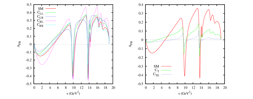
Figure 1: The FB asymmetry as a function of the dileptonic invariant mass ($s$) for various values of the Wilson coefficients. In the above plots we have chosen $|C_{LL}|=|C_{LR}|=|C_{RL}|=|C_{RR}|=3$ and $C_{T}=C_{TE}=1.5$.

As pointed out in section 1, there have been several theoretical proposals indicating that some of the new results of the $B$-factories are pointing towards the presence of weak phases in the electroweak and scalar sectors. The presence of these phases in the electroweak sector implies the possibility of $C_{LL}$, $C_{LR}$, $C_{RL}$ and $C_{RR}$ as being, in general, complex. Similarly the possibility of the presence of a phase in the scalar sector implies $C_{LRRL}$, $C_{LRLR}$, $C_{RLLR}$ and $C_{RLRL}$ as also being, in general, complex. To incorporate these possibilities in our simulations we have parameterized these coefficients as;

$$C_{X}=|C_{X}|e^{i\phi_{X}}$$ (12)

where $X$ can be $LL$, $LR$, $RL$, $RR$, $LRRL$, $LRLR$, $RLRL$ and $RLLR$.

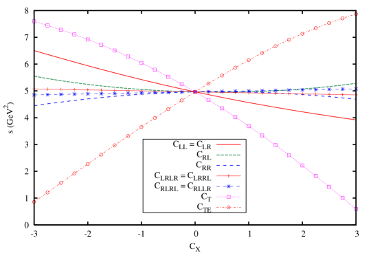
Figure 2: The Zeroes of the FB asymmetry as a function of the Wilsons. The Wilsons here are taken to be real.

The form factor definitions for $B\to K^{*}$ which we have used are given in appendix A. Finally, in our numerical analysis we have considered only the final state lepton as being the muon ($\mu$). Our reason for choosing this is due to the extreme difficulty in detecting an electron in the final state and that the branching ratio of $B\to K^{*}\ell^{+}\ell^{-}$ becomes small within the SM for $\tau$ in the final state.

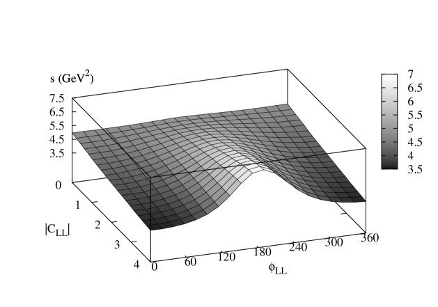
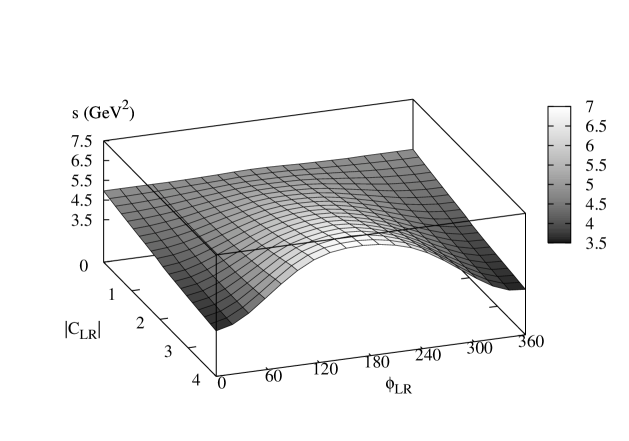
Figure 3: The Zero of the FB asymmetry as a function of the magnitude and phase of $C_{LL}$.

Figure 4: The Zero of the FB asymmetry as a function of the magnitude and phase of $C_{LR}$.

In our first set of graphs, given in Figure 1, we have plotted the FB asymmetry as a function of the dilepton invariant mass for various values of the Wilsons. Our SM value of the zero of the FB asymmetry is $s=4.94$. As can be seen from Figure 1 the value of the zero can be substantially changed for different choices of the Wilsons. We shall demonstrate this feature further later in this section.

In Figure 2 we have plotted the zero of the FB asymmetry as a function of real-valued Wilson coefficients. As can be observed from this figure the zero can show substantial modifications, especially for changes in the tensorial operators, which gives the greatest change. But as we shall soon see, substantial modifications to the FB asymmetry zeroes can arise from the other Wilsons when we include the possible new phases.

The dependence of the zero on both the magnitude and the phase of the Wilsons was next explored. Note that although all the Wilsons show changes in the zero we have only shown the results for $C_{LL}$ and $C_{LR}$, as these two Wilsons show the greatest variation. As such, in Figure 4 we have shown variation for $C_{LL}$ and in Figure 4 the dependence of the zero on the magnitude and phase of $C_{LR}$. From these figures we can not only observe the dependence of the zero on the magnitude, which further demonstrates the observations of Figure 2, but also how it can crucially depend on the phase of the Wilson. This point can be further clarified in next set of graphs.

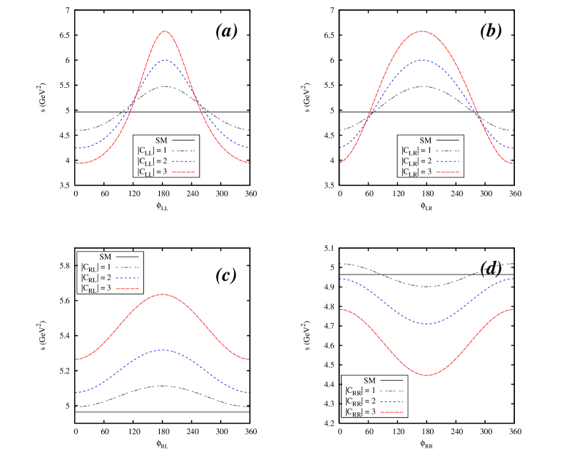
Figure 5: Plot of the zero of the FB asymmetry with the phases of the Wilsons (for different magnitudes of these Wilsons). The different panels correspond to (a) $C_{LL}$ (b) $C_{LR}$ (c) $C_{RL}$ and (d) $C_{RR}$.

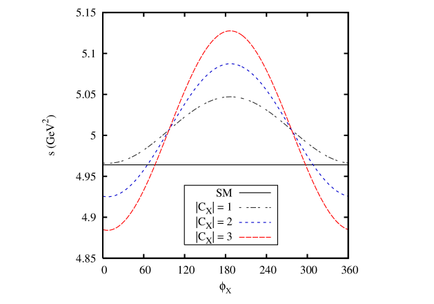
Figure 6: Plots of the zero of the FB asymmetry with the phases of various Wilsons (for different magnitudes of these Wilsons). In the above figure $X=LRLR,LRRL$.

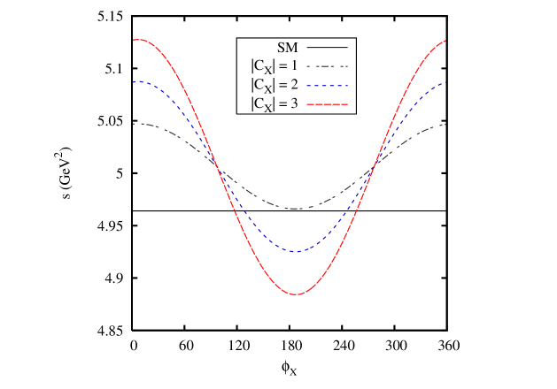
Figure 7: Plots of the zero of the FB asymmetry with the phases of various Wilsons (for different magnitudes of these Wilsons). In the above figure $X=RLLR,RLRL$.

In Figure 5 we have plotted the zero of the FB asymmetry as a function of the phases of the Wilsons for different magnitudes. This figure emphasizes how strongly the zero of the FB asymmetry depends on the phase. The variation from the SM result, in the case of $C_{LL}$ and $C_{LR}$ (which gives us the greatest variation) can change the asymmetry from 4 to 6.5, a variation of more than 60%. In Figure 6 we have plotted the zero as a function of the phase of $C_{LRLR}$ and $C_{LRRL}$. Similar graphs have been plotted in Figure 7 for $C_{RLRL}$ and $C_{RLLR}$. As can be seen from these two figures, coefficients corresponding to the scalar and electroweak operators do indeed demonstrate a dependence of the FB asymmetry on the phase. However, the dependence of the zero in the case of the electroweak operators is much greater than the scalar operators.

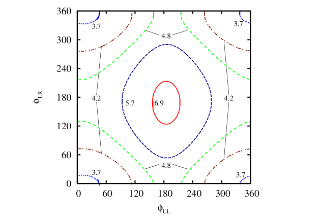
Figure 8: Contours plots for the zeroes of the FB asymmetry in the $\phi_{LL}$ and $\phi_{LR}$ plane. In this plot we have chosen $|C_{LL}|=|C_{LR}|=2$.

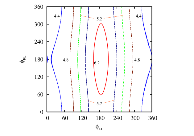
Figure 9: Contours plot for the zeroes of the FB asymmetry in the $\phi_{LL}$ and $\phi_{RL}$ plane. In this plot we have chosen $|C_{LL}|=|C_{RL}|=2$.

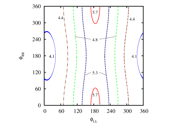
Figure 10: Contours plot for the zeroes of the FB asymmetry in the $\phi_{LL}$ and $\phi_{RR}$ plane. In this plot we have chosen $|C_{LL}|=|C_{RR}|=2$.

To illustrate our previous point further our final set of graphs, Figures 8, 9 and 10 show the contour plots of the zeroes of the FB assuming the presence of two electroweak operators now having an additional phase. As can be seen from these graphs the presence of a weak phase in the electroweak sector can give substantial deviations in the zero of FB asymmetry.

At this point we should like point out that in order to resolve the $B\to\pi\pi$ and $B\to\pi K$ puzzle Buras et al. [15] proposed the presence of a phenomenological weak phase in the electroweak penguins. This phase in effect modifies the $C_{10}$ Wilson of the SM. This modification not only increases the magnitude of $C_{10}$, by more than two, but also adds a new large phase; making the Wilson predominantly imaginary. Note that this kind of phase will not change the zero of the FB asymmetry, as within the SM the zero of the FB asymmetry does not depend on $C_{10}$. However, in general, the presence of extra phases in the electroweak sector will substantially modify the zero of the FB asymmetry.

From our analysis we have demonstrated that the zero of the FB asymmetry will not only serve as a valuable test of the SM, as emphasized in the earlier works [13, 12], but will be a useful probe of any possible new physics.

Appendix A Form Factors

The form factor definitions which we have used are as given in Ali. et al. [2];

$$F(\hat{s})=F(0)\mathrm{exp}\left(c_{1}\hat{s}+c_{2}\hat{s}^{2}\right),$$ (13)

where the values of $c_{1}$ and $c_{2}$ are given in Table 1.

	$A_{1}$	$A_{2}$	$A_{0}$	$V$	$T_{1}$	$T_{2}$	$T_{3}$
F(0)	0.337	0.282	0.471	0.457	0.379	0.379	0.260
$c_{1}$	0.602	1.172	1.505	1.482	1.519	0.517	1.129
$c_{2}$	0.258	0.567	0.710	1.015	1.030	0.426	1.128

Table 1: Form factors for the $B\to K^{*}$ transition.

Appendix B Input parameters

$m_{t}=176$ GeV   ,   $m_{c}=1.4$ GeV   ,   $m_{\mu}=0.105$ GeV

$m_{B}=5.26$ GeV   ,   $m_{b}=4.8$ GeV   ,   $sin^{2}\theta_{w}=0.23$   ,   $\alpha=1/130$   ,   $m_{K^{*}}=0.892$ GeV.

References

• [1] M. S. Alam et al. [CLEO Collaboration], Phys. Rev. Lett.  74, 2885 (1995) ; R. Ammar et al. [CLEO Collaboration], Phys. Rev. Lett.  71, 674 (1993).
• [2] A. Ali, P. Ball, L. T. Handoko and G. Hiller, Phys. Rev. D 61, 074024 (2000) [arXiv:hep-ph/9910221].
• [3] T. M. Aliev, A. Ozpineci and M. Savci, Phys. Rev. D 56, 4260 (1997) [arXiv:hep-ph/9612480] ; T. M. Aliev, M. Savci, A. Ozpineci and H. Koru, Phys. Lett. B 410, 216 (1997) [arXiv:hep-ph/9704323].
• [4] P. Ball and V. M. Braun, Phys. Rev. D 58, 094016 (1998) [arXiv:hep-ph/9805422]. D. Melikhov, N. Nikitin and S. Simula, Phys. Rev. D 57, 6814 (1998) [arXiv:hep-ph/9711362].
• [5] C. H. Chen and C. Q. Geng, Phys. Rev. D 63, 114025 (2001) [arXiv:hep-ph/0103133].
• [6] F. Kruger and L. M. Sehgal, Phys. Lett. B 380, 199 (1996) [arXiv:hep-ph/9603237].
• [7] A. S. Cornell and N. Gaur, JHEP 0309, 030 (2003) [arXiv:hep-ph/0308132] ; N. Gaur, arXiv:hep-ph/0305242 ; S. Rai Choudhury, A. Gupta and N. Gaur, Phys. Rev. D 60, 115004 (1999) [arXiv:hep-ph/9902355].
• [8] T. M. Aliev, M. K. Cakmak and M. Savci, Nucl. Phys. B 607, 305 (2001) [arXiv:hep-ph/0009133] ; T. M. Aliev, A. Ozpineci, M. Savci and C. Yuce, Phys. Rev. D 66, 115006 (2002) [arXiv:hep-ph/0208128] ; T. M. Aliev, A. Ozpineci and M. Savci, Phys. Lett. B 511, 49 (2001) [arXiv:hep-ph/0103261] ; T. M. Aliev and M. Savci, Phys. Lett. B 481, 275 (2000) [arXiv:hep-ph/0003188] ; T. M. Aliev, D. A. Demir and M. Savci, Phys. Rev. D 62, 074016 (2000) [arXiv:hep-ph/9912525] ; T. M. Aliev, C. S. Kim and Y. G. Kim, Phys. Rev. D 62, 014026 (2000) [arXiv:hep-ph/9910501] ; T. M. Aliev and E. O. Iltan, Phys. Lett. B 451, 175 (1999) [arXiv:hep-ph/9804458] ; C. H. Chen and C. Q. Geng, Phys. Rev. D 66, 034006 (2002) [arXiv:hep-ph/0207038] ; C. H. Chen and C. Q. Geng, Phys. Rev. D 66, 014007 (2002) [arXiv:hep-ph/0205306]. G. Erkol and G. Turan, Nucl. Phys. B 635, 286 (2002) [arXiv:hep-ph/0204219] ; E. O. Iltan, G. Turan and I. Turan, J. Phys. G 28, 307 (2002) [arXiv:hep-ph/0106136] ; T. M. Aliev, V. Bashiry and M. Savci, JHEP 0405, 037 (2004) [arXiv:hep-ph/0403282]. W. J. Li, Y. B. Dai and C. S. Huang, arXiv:hep-ph/0410317 ; Q. S. Yan, C. S. Huang, W. Liao and S. H. Zhu, Phys. Rev. D 62, 094023 (2000) [arXiv:hep-ph/0004262]. S. R. Choudhury, N. Gaur, A. S. Cornell and G. C. Joshi, Phys. Rev. D 68, 054016 (2003) [arXiv:hep-ph/0304084] ; S. R. Choudhury, A. S. Cornell, N. Gaur and G. C. Joshi, Phys. Rev. D 69, 054018 (2004) [arXiv:hep-ph/0307276].
• [9] A. Ali, E. Lunghi, C. Greub and G. Hiller, Phys. Rev. D 66, 034002 (2002) [arXiv:hep-ph/0112300] ; F. Kruger and E. Lunghi, Phys. Rev. D 63, 014013 (2001) [arXiv:hep-ph/0008210].
• [10] S. Rai Choudhury ,   N. Gaur  and  N. Mahajan, Phys. Rev. D 66, 054003 (2002) [arXiv:hep-ph/0203041] ; S. R. Choudhury and N. Gaur, arXiv:hep-ph/0205076 ; S. R. Choudhury and N. Gaur, arXiv:hep-ph/0207353 ; T. M. Aliev, V. Bashiry and M. Savci, Phys. Rev. D 71, 035013 (2005) [arXiv:hep-ph/0411327] ; U. O. Yilmaz, B. B. Sirvanli and G. Turan, Nucl. Phys. B 692, 249 (2004) [arXiv:hep-ph/0407006] ; U. O. Yilmaz, B. B. Sirvanli and G. Turan, Eur. Phys. J. C 30, 197 (2003) [arXiv:hep-ph/0304100] ;
• [11] S. R. Choudhury and N. Gaur, Phys. Lett. B 451, 86 (1999) [arXiv:hep-ph/9810307]. J. K. Mizukoshi, X. Tata and Y. Wang, Phys. Rev. D 66, 115003 (2002) [arXiv:hep-ph/0208078] ; T. Ibrahim and P. Nath, Phys. Rev. D 67, 016005 (2003) [arXiv:hep-ph/0208142] ; G. L. Kane, C. Kolda and J. E. Lennon, arXiv:hep-ph/0310042 ; A. J. Buras, P. H. Chankowski, J. Rosiek and L. Slawianowska, Nucl. Phys. B 659, 3 (2003) [arXiv:hep-ph/0210145] ; A. J. Buras, P. H. Chankowski, J. Rosiek and L. Slawianowska, Phys. Lett. B 546, 96 (2002) [arXiv:hep-ph/0207241] ; A. Dedes, H. K. Dreiner and U. Nierste, Phys. Rev. Lett.  87, 251804 (2001) [arXiv:hep-ph/0108037].
• [12] M. Beneke, T. Feldmann and D. Seidel, Nucl. Phys. B 612, 25 (2001) [arXiv:hep-ph/0106067] ; T. Feldmann and J. Matias, JHEP 0301, 074 (2003) [arXiv:hep-ph/0212158].
• [13] G. Burdman, Phys. Rev. D 57, 4254 (1998) [arXiv:hep-ph/9710550].
• [14] K. Anikeev et al., arXiv:hep-ph/0201071 ; J. Hewett (ed.)et al., arXiv:hep-ph/0503261 ; P. Ball et al., arXiv:hep-ph/0003238 ; A. G. Akeroyd et al. [SuperKEKB Physics Working Group], arXiv:hep-ex/0406071 ; S. Hashimoto (ed.)et al., KEK-REPORT-2004-4 ;
• [15] A. J. Buras and R. Fleischer, Eur. Phys. J. C 16, 97 (2000) [arXiv:hep-ph/0003323].
• [16] A. J. Buras, R. Fleischer, S. Recksiegel and F. Schwab, Phys. Rev. Lett.  92, 101804 (2004) [arXiv:hep-ph/0312259]; Nucl. Phys. B 697, 133 (2004) [arXiv:hep-ph/0402112]; Eur. Phys. J. C 32, 45 (2003) [arXiv:hep-ph/0309012] ; T. Yoshikawa, Phys. Rev. D 68, 054023 (2003) [arXiv:hep-ph/0306147] ; M. Gronau and J. L. Rosner, Phys. Lett. B 572, 43 (2003) [arXiv:hep-ph/0307095] ; M. Beneke and M. Neubert, Nucl. Phys. B 675, 333 (2003) [arXiv:hep-ph/0308039].
• [17] S. R. Choudhury, A. S. Cornell, N. Gaur and G. C. Joshi, arXiv:hep-ph/0504193.
• [18] A. S. Cornell and N. Gaur, JHEP 0502, 005 (2005) [arXiv:hep-ph/0408164].
• [19] S. Rai Choudhury, N. Gaur and A. S. Cornell, Phys. Rev. D 70, 057501 (2004) [arXiv:hep-ph/0402273];
• [20] G. Buchalla, G. Hiller and G. Isidori, Phys. Rev. D 63, 014015 (2001) [arXiv:hep-ph/0006136] ; G. Colangelo and G. Isidori, JHEP 9809, 009 (1998) [arXiv:hep-ph/9808487] ; A. J. Buras and L. Silvestrini, Nucl. Phys. B 546, 299 (1999) [arXiv:hep-ph/9811471] ; G. Isidori, arXiv:hep-ph/0009024.