UH-511-1069-05 The electron energy spectrum in muon decay through ${\cal O}(\alpha^{2})$

Abstract

We compute the complete ${\cal O}(\alpha^{2})$ QED corrections to the electron energy spectrum in unpolarized muon decay, including the full dependence on the electron mass. Our calculation reduces the theoretical uncertainty on the electron energy spectrum well below $10^{-4}$, the precision anticipated by the TWIST experiment at TRIUMF, which is currently performing this measurement. For this calculation, we extend techniques we have recently developed for performing next-to-next-to-leading order computations to handle the decay spectra of massive particles. Such an extension enables further applications to precision predictions for $b$, $t$, and Higgs differential decay rates.

I Introduction

The decay of a muon into an electron and a pair of neutrinos, $\mu\rightarrow e\nu_{\mu}\bar{\nu}_{e}$, occupies an important role in particle physics. The measurement of the muon lifetime Bardin:1984ie leads to the most accurate determination of the Fermi coupling constant, $G_{F}$. The muon anomalous magnetic moment is one of the most precisely measured quantities in nature Bennett:2002jb ; Brown:2001mg , and provides important constraints on physics beyond the Standard Model (SM) czar . Searches for lepton flavor-violating decays of the muon, such as $\mu\rightarrow e\gamma$ and $\mu\rightarrow eee$, constrain the flavor sector of many SM extensions kuno .

The calculations of radiative corrections to muon decay have a long and storied history kinoshita . The one-loop QED corrections were first performed within the Fermi theory of weak interactions in the 1950s firstcalcs . The cancellation of mass singular terms such as ${\rm ln}(m_{\mu}/m_{e})$ in the total rate, but not in distributions such as the electron energy spectrum, led to the development of the Kinoshita-Lee-Nauenberg theorem, which explains how to construct “infrared-safe” observables in quantum field theory where such effects cancel KLN . The calculation of the full one-loop corrections in the ${\rm SU(2)}\times{\rm U(1)}$ theory of the electroweak interactions was one of the first such computations performed EW1loop . The full two-loop corrections to the muon lifetime in the Fermi model, needed for a precision determination of $G_{F}$, were completed several years ago QED2loop ; recently, the two-loop results in the full electroweak theory were obtained twoloopew .

Muon decay continues to be of interest in particle physics. The TWIST experiment at TRIUMF TWIST measures the electron energy and angular distributions in polarized muon decay; the first results were recently reported in twistik . It is anticipated that TWIST will eventually measure the Michel parameters Michel , which describe muon decay for the most general form of the four-fermion interaction, to a precision of $\approx 10^{-4}$. This significantly increases the sensitivity of muon decay to deviations arising from new physics. For example, the lower bound on the mass of the $W_{R}$ in the manifest left-right symmetric model is improved from $M_{W_{R}}>400$ GeV to $M_{W_{R}}>800$ GeV, competitive with limits coming from the Tevatron, while the bounds on the left-right mixing parameter $\zeta$ are improved by nearly an order of magnitude kuno . Such precision requires a careful consideration of the higher order corrections. As noted above, the radiative corrections to quantities such as the electron energy distribution contain large logarithms of the form ${\rm ln}(m_{\mu}/m_{e})$, which enhances their effect. The presence of mass singularities makes it impossible to compute the radiative corrections to the electron energy spectrum by neglecting the mass of the electron from the very beginning, the approximation that has been used successfully in the calculation of QED corrections to the muon lifetime QED2loop . This feature makes the calculation of the ${\cal O}(\alpha^{2})$ corrections to the spectrum a challenging problem that has defied solution for many years.

It was realized recently that the logarithmically enhanced parts of the second order QED corrections can be computed using the factorization of mass singularities traditionally discussed in the context of QCD. In this way, the two-loop corrections with a double logarithmic enhancement, ${\cal O}(\alpha^{2}{\rm ln}^{2}(m_{\mu}/m_{e}))$, were calculated in Arbuzov:2002pp , and the singly-enhanced ${\cal O}(\alpha^{2}{\rm ln}(m_{\mu}/m_{e}))$ terms were computed in Arbuzov:2002cn . At the midpoint of the electron energy spectrum, the sizes of these two terms are respectively $-7\times 10^{-4}$ and $3\times 10^{-4}$. There are two interesting features of these results. The first is that the corrections are larger than the anticipated experimental precision, $10^{-4}$. The second is that the single-logarithmic terms are not a full factor of ${\rm ln}(m_{\mu}/m_{e})\approx 5$ times smaller than the double-logarithmic terms, indicating that the naive power-counting based on the size of this logarithm might not hold. Both of these facts render a full calculation of the ${\cal O}(\alpha^{2})$ corrections desirable.

In this paper we compute the ${\cal O}(\alpha^{2})$ QED corrections to the electron energy spectrum in muon decay. The full dependence on the electron mass is retained. We use a method of performing next-to-next-to-leading-order (NNLO) calculations developed by us in a recent series of papers secdecomp . Our technique features an automated extraction and numerical cancellation of divergences which appear as poles in the dimensional regularization parameter $\epsilon=(4-d)/2$. In muon decay, ultraviolet divergences and divergences arising from soft photon emissions appear as $1/\epsilon$ poles, while emission of photons along the electron direction is regulated by the finite mass of the electron and leads to logarithms of the ratio of the muon to electron mass, ${\rm ln}(m_{\mu}/m_{e})$. From the technical point of view, the fact that the electron mass plays the role of the collinear regulator leads to some differences as compared to calculations with only massless particles. Having masses as regulators reduces the complexity of the analytic structures which must be integrated over multi-particle phase-spaces or over virtual loop momenta. However, issues of numerical stability appear since multi-dimensional integrals are regulated by $(m_{e}/m_{\mu})^{2}\sim 10^{-5}$. We find that the presence of a mass regulator significantly simplifies the treatment of real emission processes of the type $\mu\to\nu_{\mu}\bar{\nu}_{e}e+\gamma\gamma$; however, the computation of virtual corrections becomes more complex, compared to a purely massless case. We describe these and other technical issues in detail in the main body of the paper.

Many other physics applications require computations of higher order corrections to the decay spectra of massive particles. For example, the structure of the ${\cal O}(\alpha^{2})$ corrections to muon decay is identical to the ${\cal O}(\alpha_{s}^{2})$ QCD corrections to semi-leptonic $b\rightarrow u$ and $b\rightarrow c$ transitions, which are used to extract the CKM matrix elements $|V_{ub}|$ and $|V_{cb}|$, the $b$-quark mass and other important parameters of Heavy Quark Effective Theory bphys . The calculation of QED radiative corrections to the electron energy spectrum discussed in this paper can be easily extended to obtain differential results for semi-leptonic $b$-decays at NNLO. In fact, some of the technical issues become simpler for $b$-decays, particularly $b\rightarrow c$. In this case, collinear singularities are regulated by the factor $(m_{c}/m_{b})^{2}\approx 4\times 10^{-2}$, rather than $(m_{e}/m_{\mu})^{2}\approx 10^{-5}$, leading to more stable numerics. Precise predictions for heavy particle decay spectra will also be important for measurements at both the LHC and a future linear collider. Both experiments will search for anomalous top quark couplings through final-state distributions in its decay $t\rightarrow bW$, and will determine the CP properties of any scalar boson discovered through angular properties of such decays as $\phi\rightarrow ZZ,WW,f\bar{f}$ tophiggs . The techniques required to analyze higher-order corrections to these decay modes are very similar to those presented here.

This paper is organized as follows. In the next Section we introduce our notation and discuss general aspects of the computation of the electron energy spectrum. In Section III we describe our computation of the NNLO QED corrections. In Section IV we discuss our results. Finally, we present our conclusions.

II Notation and setup

We discuss in this Section some basic notation needed to describe muon decay. We begin with the Lagrangian

$${\cal L}={\cal L}_{QED}+{\cal L}_{F}.$$ (1)

${\cal L}_{QED}$ contains the kinetic terms for the fermions and photons, along with the QED interactions,

$${\cal L}_{QED}=-\frac{1}{4}F_{\mu\nu}F^{\mu\nu}+\sum_{f}\bar{\psi}_{f}\left[i\not\!D-m_{f}\right]\psi_{f},$$ (2)

while ${\cal L}_{F}$ contains the Fermi interaction,

$${\cal L}_{F}=-2\sqrt{2}G_{F}\left[\bar{\psi}_{\nu_{\mu}}\gamma^{\rho}P_{L}\psi_{\mu}\right]\left[\bar{\psi}_{e}\gamma_{\rho}P_{L}\psi_{\nu_{e}}\right].$$ (3)

Here, $P_{L}=(1-\gamma_{5})/2$ is the usual left-handed projection operator. The Fermi Lagrangian can be Fierz rearranged into the following form:

$${\cal L}_{F}\rightarrow-2\sqrt{2}G_{F}\left[\bar{\psi}_{e}\gamma^{\rho}P_{L}\psi_{\mu}\right]\left[\bar{\psi}_{\nu_{\mu}}\gamma^{\rho}P_{L}\psi_{\nu_{e}}\right].$$ (4)

The QED corrections to this Lagrangian are finite to all orders in $\alpha$ fermiqed after the fermion mass renormalization is included. Since the QED corrections do not affect the neutrino part of this Lagrangian, and experiments do not probe properties of the neutrinos, they can be integrated out to produce an effective $\mu-e$ current. We demonstrate this here. We first note that since QED interactions only affect the leftmost fermion bilinear of Eq. 4, we can write the squared matrix element for the process $\mu\rightarrow e\nu_{e}\nu_{\mu}+X$ as

$$|{\cal M}|^{2}=|{\cal M}^{\rho\sigma}_{\mu\rightarrow e+X}|^{2}\times{\rm Tr}\left[\not\!p_{\nu_{e}}\gamma_{\rho}\not\!p_{\nu_{\mu}}\gamma_{\sigma}P_{L}\right].$$ (5)

${\cal M}^{\rho\sigma}_{\mu\rightarrow e+X}$ denotes the matrix element formed from the leftmost bilinear of Eq. 4 together with any QED corrections. Eq.(5) must be integrated over the appropriate phase-space to obtain the electron energy spectrum:

$$\frac{d\Gamma}{dx} = \int[d\Pi_{\mu\rightarrow e\nu\nu+X}]|{\cal M}|^{2}$$ (6)

$$= \int dp_{\rm nt}^{2}\int[d\Pi_{\mu\rightarrow ep_{\rm nt}+X}]|{\cal M}^{\rho\sigma}_{\mu\rightarrow e+X}|^{2}\times\int[d\Pi_{p_{\rm nt}\rightarrow\nu_{e}\nu_{\mu}}]{\rm Tr}\left[\not\!p_{\nu_{e}}\gamma_{\rho}\not\!p_{\nu_{\mu}}\gamma_{\sigma}P_{L}\right],$$

where $x=2E/m_{\mu}$ and $E$ is the electron energy. In the second line, we have partitioned the phase-space so that the muon first decays into an electron, additional radiation denoted by $X$, and a massive state with momentum

$$p_{\rm nt}=p_{\mu}-p_{e}-p_{X}.$$ (7)

This massive state then decays into the muon and electron neutrinos. The neutrino portion of the phase-space can be integrated over to obtain

$$\int[d\Pi_{p_{\rm nt}\rightarrow\nu_{e}\nu_{\mu}}]{\rm Tr}\left[\not\!p_{\nu_{e}}\gamma_{\rho}\not\!p_{\nu_{\mu}}\gamma_{\sigma}P_{L}\right]=T_{\rho\sigma}^{\rm nt},$$ (8)

with

$$T_{\rho\sigma}^{\rm nt}=-\frac{\pi p_{\rm nt}^{2}}{3(2\pi)^{d-1}}\left[g_{\rho\sigma}-\frac{p_{\rm nt,\rho}p_{\rm nt,\sigma}}{p_{\rm nt}^{2}}\right],$$ (9)

giving the expression for the decay spectrum

$$\frac{d\Gamma}{dx}=\int dp_{\rm nt}^{2}\int[d\Pi_{\mu\rightarrow ep_{\rm nt}+X}]|{\cal M}^{\rho\sigma}_{\mu\rightarrow e+X}|^{2}T_{\rho\sigma}^{\rm nt}.$$ (10)

Since, up to an overall numerical factor, $T_{\rho\sigma}^{\rm nt}$ coincides with the polarization density matrix of a vector boson with mass $p_{\rm nt}^{2}$, we can interpret Eq. 10 as the emission of such a boson in the $\mu-e$ transition. A sample of the diagrams that appear in this description are shown in Fig. 1.

Figure 1: A sample of LO and NLO diagrams which appear for the effective $\mu-e$ current after the neutrinos are integrated out. The factor to be associated with the effective $\mu-e$ vertex after squaring the matrix elements is given in Eq. 9.

Since we are regulating divergences in dimensional regularization, we briefly discuss our treatment of the $\gamma_{5}$ which appears in $P_{L}$ in Eq. 4. Our conclusion is that a naive anti-commuting $\gamma_{5}$ can be used, and fermion traces containing an odd number of $\gamma_{5}$ matrices do not contribute. This follows from the observation that the tensor $T^{\rho\sigma}_{\rm nt}$ is symmetric under $\rho\leftrightarrow\sigma$; a contribution containing an odd number of $\gamma_{5}$ matrices will produce a form factor containing the completely anti-symmetric Levi-Cevita tensor and will vanish when contracted with $T^{\rho\sigma}_{\rm nt}$.

We now discuss the form in which we will present our results. We parameterize the electron energy spectrum with the variable $x=2E/m_{\mu}$ which lies in the range

$$\frac{2m_{e}}{m_{\mu}}\leq x\leq 1+\frac{m_{e}^{2}}{m_{\mu}^{2}}.$$ (11)

We write the differential decay rate as

$$\frac{d\Gamma}{dx}=\frac{G_{F}^{2}m_{\mu}^{5}}{192\pi^{3}}\sum_{n=0}\left(\frac{\alpha}{\pi}\right)^{n}f^{(n)}(x).$$ (12)

The LO and NLO results were computed in firstcalcs ; they can be obtained in a convenient form in QED2loop ; arbuzov1l . The logarithmically enhanced contributions to $f^{(2)}(x)$ can be obtained from Arbuzov:2002pp ; Arbuzov:2002cn . The calculation of $f^{(2)}(x)$ beyond the logarithmic approximation, and including the full dependence on the electron mass, is the main subject of this paper.

III NNLO corrections

In this Section we discuss our computation of the NNLO corrections to the electron energy spectrum. We give a brief overview of the technical aspects of the calculation and then describe in detail the computation of double real emission, one-loop virtual corrections to a single photon emission, and two-loop virtual corrections.

III.1 Overview of NNLO corrections

We first present a brief overview of the various components of the NNLO corrections. The differential decay rate contains a sum over several distinct components,

$$\frac{d\Gamma}{dx}=\sum_{Y}\frac{d\Gamma_{Y}}{dx},$$ (13)

where each $d\Gamma_{Y}/dx$ is separately divergent and must be combined with the other components to produce a finite result. Our method of calculation follows the technique outlined in secdecomp . We regulate both infrared and ultraviolet divergences in dimensional regularization, setting the space-time dimension $d=4-2\epsilon$, and produce an expansion

$$\frac{d\Gamma_{Y}}{dx}=\sum_{i=2}^{0}\frac{A^{Y}_{i}(p_{\mu},p_{e})}{\epsilon^{i}},$$ (14)

where the $A^{Y}_{i}$ are functions non-singular everywhere in phase-space. Since the $A^{Y}_{i}$ are non-singular, they can be computed numerically in four dimensions. The expressions for the $d\Gamma_{Y}/dx$ can be combined, and the poles in $\epsilon$ can be cancelled numerically. We must produce such an expansion for the following components.

1. The real radiation corrections involve decays with two additional particles radiated into the final state. The two relevant processes are $\mu\rightarrow e\nu\nu+\gamma\gamma$ and $\mu\rightarrow e\nu\nu+e^{+}e^{-}$. The first one begins at $1/\epsilon^{2}$, with the singularities coming from the phase-space regions where the photon energies vanish, while the second is finite. To handle these corrections, we use the techniques presented in secdecomp . We describe our phase-space parameterizations and discuss the extraction of singularities in Subsection III.2.

2. The real-virtual component includes the 1-loop virtual corrections to the process $\mu\rightarrow e\nu\nu+\gamma$, and contributes beginning at $1/\epsilon^{2}$. We use a hybrid approach combining both analytical and numerical techniques to compute this component. We first use integration-by-parts identities and recurrence relations tkachov to reduce the corrections to a small set of master integrals. The recurrence relations are solved using the algorithm described in laporta and implemented in air . We then solve for the master integrals numerically by applying the techniques of secdecomp to their Feynman parameter representation. We discuss the details of this method, including how we handle imaginary components of the loop integrals, in Subsection III.3.

3. The virtual-virtual corrections contain the interference of two-loop virtual corrections to $\mu\rightarrow e\nu\nu$ with tree-level diagrams. These begin at $1/\epsilon^{2}$. We deal with these completely numerically by applying the techniques of secdecomp directly to their Feynman parameter representation. This numerical method of computing virtual corrections was pioneered in Binoth:2000ps ; Binoth:2003ak . We apply it here for the first time in a fully realistic calculation, which includes tensor integrals and several mass scales. We discuss the details of this calculation in Subsection III.4.

4. We must include the square of the NLO virtual corrections, which contribute at ${\cal O}(\alpha^{2})$ and produce poles beginning at $1/\epsilon^{2}$. Since the computation of this component can be performed with standard techniques, we do not discuss it further.

5. We must include both fermion mass renormalization, and external wave-function renormalization. We renormalize in the on-shell scheme. The renormalization is performed by multiplying the LO and NLO results by the factor $Z_{2}^{e}\times Z_{2}^{\mu}$, and by inserting the muon and electron mass counterterms into the NLO diagrams. Therefore, the mass counter-term is needed through ${\cal O}(\alpha)$ only. For a fermion of mass $m$, the renormalization constants are broad ; Melnikov:2000zc

   $$Z_{2} = 1+\sum_{n=1}\left[\frac{\alpha}{\pi}\frac{\Gamma(1+e)m^{-2\epsilon}}{(4\pi)^{-\epsilon}}\right]^{n}Z_{2}^{(n)},$$

   $$Z_{2}^{(1)} = -\frac{3}{4\epsilon}-\frac{1}{1-2\epsilon},~{}~{}~{}Z_{2}^{(2)}=\frac{9}{32\epsilon^{2}}+\frac{51}{64\epsilon}+\frac{433}{128}-\frac{3}{2}\zeta(3)+\pi^{2}{\rm ln}(2)-\frac{13}{16}\pi^{2},$$

   $$\delta m = m_{\rm bare}-m=m(Z_{m}-1)=\frac{\alpha}{\pi}\frac{\Gamma(1+e)m^{1-2\epsilon}}{(4\pi)^{-\epsilon}}Z_{2}^{(1)}.$$ (15)

   We note that contributions which arise from a closed fermion loop inserted into a 1-loop self-energy diagram, which appear at ${\cal O}(\alpha^{2})$, have been removed from these formulae; they are more naturally included in the contribution discussed in the following item.

6. Finally, we must include vacuum polarization corrections, in which a muon or electron loop is inserted into a 1-loop diagram. These include the insertion of a closed fermion loop into a 1-loop vertex diagram, and insertions into external leg self-energy corrections, which contribute to the muon and electron wave function renormalization constants. These corrections form a finite subset. They can be computed using dispersive techniques, as discussed in vanRitbergen:1998hn ; Davydychev:2000ee , where their contribution to the muon lifetime and electron energy spectrum are computed. Since these corrections are discussed in the literature, and can be computed with standard techniques, we do not discuss them further.

After combining items $1-6$, both ultraviolet and infrared divergences cancel, leaving a finite result. This completes the brief summary of the terms which enter the ${\cal O}(\alpha^{2})$ corrections; we now begin the technical discussion of their computation.

III.2 Real radiation corrections

We first discuss the contribution of the real radiation processes $\mu\rightarrow e\nu\nu+\gamma\gamma$ and $\mu\rightarrow e\nu\nu+e^{+}e^{-}$. A sample of the diagrams that contribute to these processes is shown in Fig. 2. They produce a contribution to the differential decay rate of the form

$$\frac{d\Gamma_{RR}}{dx}=\int dp_{\rm nt}^{2}\int[d\Pi_{\mu\rightarrow ep_{\rm nt}+X}]|{\cal M}^{\rho\sigma}_{\mu\rightarrow e+X}|^{2}T^{\rho\sigma}_{\rm nt}.$$ (16)

Figure 2: Sample diagrams which contribute to $\mu\rightarrow e\nu\nu+\gamma\gamma$ (left) and $\mu\rightarrow e\nu\nu+e^{+}e^{-}$ (right)

In order to perform the integration in Eq. 16, we must discuss both our phase-space parameterizations and the singularity structure of the matrix elements. Denoting the radiation momenta by $p_{\gamma 1}$, $p_{\gamma 2}$, $p_{e^{-}1}$, $p_{e^{+}2}$, we find the following denominators for each process:

• $\mu\rightarrow e\nu\nu+\gamma\gamma$: $d^{\gamma}_{\mu 1}=(p_{\mu}-p_{\gamma 1})-m_{\mu}^{2}$, $d^{\gamma}_{\mu 2}$, $d^{\gamma}_{e1}=(p_{e}+p_{\gamma 1})-m_{e}^{2}$, $d^{\gamma}_{e2}$, $d^{\gamma}_{\mu 12}=(p_{\mu}-p_{\gamma 1}-p_{\gamma 2})-m_{\mu}^{2}$, $d^{\gamma}_{e12}=(p_{e}+p_{\gamma 1}+p_{\gamma 2})-m_{e}^{2}$;

• $\mu\rightarrow e\nu\nu+e^{+}e^{-}$: $d^{e}_{12}=(p_{e^{-}1}+p_{e^{+}2})^{2}$, $d^{e}_{e2}=(p_{e}+p_{e^{+}2})^{2}$, $d^{e}_{\mu 12}=(p_{\mu}-p_{e^{-}1}-p_{e^{+}2})^{2}-m_{\mu}^{2}$, $d^{e}_{\mu e2}=(p_{\mu}-p_{e}-p_{e^{+}2})^{2}-m_{\mu}^{2}$, $d^{e}_{e12}=(p_{e}+p_{e^{-}1}+p_{e^{+}2})^{2}-m_{e}^{2}$.

We first discuss our phase-space representation for the photon radiation process, which takes the form

$$\int dp_{\rm nt}^{2} \int[d\Pi_{\mu\rightarrow ep_{\rm nt}+X}]=\frac{1}{(2\pi)^{3d-4}}\int ds_{\rm nt}\int d^{d}p_{\rm nt}d^{d}p_{e}d^{d}p_{\gamma 1}d^{d}p_{\gamma 2}$$ (17)

$$\times \delta(p_{\rm nt}^{2}-s_{\rm nt})\delta(p_{e}^{2}-m_{e}^{2})\delta(p_{\gamma 1}^{2})\delta(p_{\gamma 2}^{2})\delta^{(d)}(p_{\mu}-p_{e}-p_{\gamma 1}-p_{\gamma 2}-p_{\rm nt}),$$

where the restriction of the electron energy fraction $x$ is understood in the rightmost equation. It is convenient to evaluate this in the rest frame of the muon and to choose the $z$-axis along the electron direction. In this frame, the momenta are

$$p_{\mu} = \left(m_{\mu},0,0,0\right),\;\;\;p_{e}=\left(E_{e},0,0,\beta E_{e}\right),$$

$$p_{\gamma 1} = \left(E_{1},E_{1}s_{1},0,E_{1}c_{1}\right),\;\;\;p_{\gamma 2}=\left(E_{2},E_{2}s_{2}c_{\phi},E_{2}s_{2}s_{\phi},E_{2}c_{2}\right),$$ (18)

where $E_{e}$, $E_{1}$, and $E_{2}$ denote energies, $s_{1}$, $s_{2}$, $c_{1}$, and $c_{2}$ respectively denote sines and cosines of polar angles, and $s_{\phi}$, $c_{\phi}$ denote the sine and cosine of the azimuthal angle. Following secdecomp , we map this to the unit hypercube, and obtain

$$N_{\gamma} \int_{0}^{1}d\lambda_{1}d\lambda_{2}d\lambda_{3}d\lambda_{4}d\lambda_{5}\,\kappa_{12}^{-2+2\epsilon}(1+\delta^{2}-x)^{4-4\epsilon}(1-\lambda_{1})^{3-4\epsilon}[\beta x]^{1-2\epsilon}$$ (19)

$$\times\left[\lambda_{2}(1-\lambda_{2})\right]^{1-2\epsilon}\left[\lambda_{3}\lambda_{4}(1-\lambda_{3})(1-\lambda_{4})\right]^{-\epsilon}\left[\lambda_{5}(1-\lambda_{5})\right]^{-1/2-\epsilon},$$

where

$$\delta = m_{e}/m_{\mu},\;\;\;c_{1}=2\lambda_{3}-1,\;\;\;c_{2}=2\lambda_{4}-1,\;\;\;c_{\phi}=2\lambda_{5}-1,$$

$$E_{e} = x/2,\;\;\;E_{1}=\frac{\lambda_{2}(1-\lambda_{1})(1+\delta^{2}-x)}{2\kappa_{1}},\;\;\;E_{2}=\frac{\kappa_{1}(1-\lambda_{2})(1-\lambda_{1})(1+\delta^{2}-x)}{2\kappa_{12}},$$

$$N_{\gamma} = \frac{\Omega_{d-1}\Omega_{d-2}\Omega_{d-3}}{2^{7}(2\pi)^{3d-4}},\;\;\;\Omega_{d}=\frac{2\pi^{d/2}}{\Gamma(d/2)},\;\;\;s_{\rm nt}=\lambda_{1}(1+\delta^{2}-x),\;\;\;\kappa_{1}=1-\frac{x}{2}(1-\beta c_{1})$$

$$\kappa_{12} = \kappa_{1}-\frac{\kappa_{1}x}{2}(1-\beta c_{2})-\frac{\lambda_{2}(1-\lambda_{1})(1+\delta^{2}-x)(1-\vec{n}_{1}\cdot\vec{n}_{2})}{2},$$

$$\beta = \sqrt{1-4\delta^{2}/x^{2}},\;\;\;\vec{n}_{1}\cdot\vec{n}_{2}=c_{1}c_{2}+s_{1}s_{2}c_{\phi}.$$ (20)

We have removed the integration over the energy fraction $x$, and have set the scale $m_{\mu}=1$; it can be restored with dimensional analysis. The matrix element denominators become

$$d^{\gamma}_{\mu 1} = \frac{-\lambda_{2}(1-\lambda_{1})(1+\delta^{2}-x)}{\kappa_{1}},\;\;\;d^{\gamma}_{\mu 2}=\frac{-\kappa_{1}(1-\lambda_{2})(1-\lambda_{1})(1+\delta^{2}-x)}{\kappa_{12}},$$

$$d^{\gamma}_{e1} = \frac{x\lambda_{2}(1-\lambda_{1})(1+\delta^{2}-x)(1-\beta c_{1})}{2\kappa_{1}},\;\;\;d^{\gamma}_{e2}=\frac{x\kappa_{1}(1-\lambda_{2})(1-\lambda_{1})(1+\delta^{2}-x)(1-\beta c_{2})}{2\kappa_{12}},$$

$$d^{\gamma}_{\mu 12} = -(1-\lambda_{1})(1+\delta^{2}-x)\left\{1+\frac{x\lambda_{2}(1-\beta c_{1})}{2\kappa_{1}}+\frac{x\kappa_{1}(1-\lambda_{2})(1-\beta c_{2})}{2\kappa_{12}}\right\},$$

$$d^{\gamma}_{e12} = (1-\lambda_{1})(1+\delta^{2}-x)\left\{-1+\frac{\lambda_{2}}{\kappa_{1}}+\frac{\kappa_{1}(1-\lambda_{2})}{\kappa_{12}}\right\}.$$ (21)

We note that all the divergences are produced by the overall multiplicative factors of $(1-\lambda_{1})$, $\lambda_{2}$, and $(1-\lambda_{2})$; the bracketed terms in $d^{\gamma}_{\mu 12}$ and $d^{\gamma}_{e12}$ are finite for values of $x$ away from its boundaries. In the language of secdecomp , all singularities are factorizable; when the denominators are combined with the phase-space in Eq. 19, the form of Eq. 14 can be produced by expanding in plus distributions:

$$\lambda^{-1+e} = \frac{1}{\epsilon}\delta(\lambda)+\sum_{n=0}\left[\frac{{\rm ln}^{n}(\lambda)}{\lambda}\right]_{+}\frac{\epsilon^{n}}{n!},$$ (22)

$$\int_{0}^{1}d\lambda\,f(\lambda)\left[\frac{{\rm ln}^{n}(\lambda)}{\lambda}\right]_{+}=\int_{0}^{1}d\lambda\,\frac{f(\lambda)-f(0)}{\lambda}\,{\rm ln}^{n}(\lambda).$$

We must now discuss our phase-space representation for the process $\mu\rightarrow e\nu\nu+e^{+}e^{-}$, which takes the form

$$\int dp_{\rm nt}^{2} \int[d\Pi_{\mu\rightarrow ep_{\rm nt}+X}]=\frac{1}{(2\pi)^{3d-4}}\int ds_{\rm nt}\int d^{d}p_{\rm nt}d^{d}p_{e}d^{d}p_{e^{-}1}d^{d}p_{e^{+}2}\,\delta(p_{\rm nt}^{2}-s_{\rm nt})$$ (23)

$$\times \delta(p_{e}^{2}-m_{e}^{2})\delta(p_{e^{-}1}^{2}-m_{e}^{2})\delta(p_{e^{+}2}^{2}-m_{e}^{2})\delta^{(d)}(p_{\mu}-p_{e}-p_{e^{-}1}-p_{e^{+}2}-p_{\rm nt}).$$

It is convenient to view this decay as occurring iteratively; first, the muon decays into an electron and a massive “particle” with momentum $p_{\rm nt}+p_{e^{-}1}+p_{e^{+}2}$. This massive particle then decays into $p_{e^{-}1}$ and another massive particle with momentum $p_{\rm nt}+p_{e^{+}2}$, which finally decays into $p_{e^{+}2}$ and the neutrino pair. This motivates the following decomposition of the phase-space:

$$\frac{1}{(2\pi)^{3d-4}}\int ds_{\rm nt}ds_{\rm nt12}ds_{\rm nt2}\,I_{1}I_{2}I_{3},$$ (24)

where

$$I_{1} = \int d^{d}p_{e}d^{d}p_{\rm nt12}\,\delta(p_{e}^{2}-m_{e}^{2})\,\delta(p_{\rm nt12}^{2}-s_{\rm nt12})\,\delta^{(d)}(p_{\mu}-p_{e}-p_{\rm nt12}),$$

$$I_{2} = \int d^{d}p_{e^{-}1}d^{d}p_{\rm nt2}\,\delta(p_{e^{-}1}^{2}-m_{e}^{2})\,\delta(p_{\rm nt2}^{2}-s_{\rm nt2})\,\delta^{(d)}(p_{\rm nt12}-p_{e^{-}1}-p_{\rm nt2}),$$

$$I_{3} = \int d^{d}p_{e^{+}2}d^{d}p_{\rm nt}\,\delta(p_{e^{+}2}^{2}-m_{e}^{2})\,\delta(p_{\rm nt}^{2}-s_{\rm nt})\,\delta^{(d)}(p_{\rm nt2}-p_{e^{+}2}-p_{\rm nt}).$$ (25)

We evaluate $I_{1}$, $I_{2}$, and $I_{3}$ in the rest frame of the massive “particle” that defines each phase-space. Doing so yields the following expression:

$$N_{ee} \int_{0}^{1}d\lambda_{1}d\lambda_{2}d\lambda_{3}d\lambda_{4}d\lambda_{5}\,\frac{\Delta_{34}\left(\sqrt{1+\delta^{2}-x}-2\delta\right)^{2}}{\sqrt{s_{\rm nt12}s_{\rm nt2}}}\left[\beta^{3}xE_{2}E_{3}\right]^{1-2\epsilon}$$ (26)

$$\times\left[\lambda_{3}\lambda_{4}(1-\lambda_{3})(1-\lambda_{4})\right]^{-\epsilon}\left[\lambda_{5}(1-\lambda_{5})\right]^{-1/2-\epsilon},$$

where

$$N_{ee} = \frac{\Omega_{d-1}\Omega_{d-2}\Omega_{d-3}}{2^{5+4\epsilon}(2\pi)^{3d-4}},\;\;\;E_{2}=\frac{s_{\rm nt12}+\delta^{2}-s_{\rm nt2}}{2\sqrt{s_{\rm nt12}}},\;\;\;E_{3}=\frac{s_{\rm nt2}+\delta^{2}-s_{\rm nt}}{2\sqrt{s_{\rm nt2}}},\;\;\;$$

$$s_{\rm nt12} = 1+\delta^{2}-x,\;\;\;s_{\rm nt}=\lambda_{1}\left(\sqrt{1+\delta^{2}-x}-2\delta\right)^{2},\;\;\;s_{\rm nt2}=\Delta_{34}\lambda_{2}+L_{34},$$

$$\Delta_{34} = \left(\sqrt{s_{\rm nt12}}-\delta\right)^{2}-\left(\sqrt{s_{\rm nt}}+\delta\right)^{2},\;\;\;L_{34}=\left(\sqrt{s_{\rm nt12}}-\delta\right)^{2},$$

$$c_{2} = 2\lambda_{3}-1,\;\;\;c_{3}=2\lambda_{4}-1,\;\;\;c_{\phi}=2\lambda_{5}-1.$$ (27)

$c_{2}$ is the polar angle of $p_{e^{-}1}$ within the frame of $I_{2}$, while $c_{3}$ and $c_{\phi}$ are respectively the polar and azimuthal angles of $p_{e^{+}2}$ within $I_{3}$. To obtain the invariant masses that appear in the matrix elements, we must Lorentz transform the vectors $p_{\mu}$, $p_{e}$, $p_{e^{-}1}$, and $p_{e^{+}2}$ between the frames defined by the three phase-spaces. We note that all of the denominators that appear in the matrix elements are regulated by $\delta$, and therefore the process $\mu\rightarrow e\nu\nu+e^{+}e^{-}$ is finite. It is sufficient to set $\epsilon=0$ in Eq. 26 and to perform the numerical integration of the corresponding matrix element in four dimensions.

III.3 Virtual corrections to single photon emission

Figure 3: Sample diagrams which contribute to $\mu\rightarrow e\nu\nu+\gamma$

Here we discuss the one-loop virtual correction to the process $\mu\to e\nu\nu+\gamma$; some diagrams that must be considered are shown in Fig. 3. This computation is conveniently performed by a combination of analytical and numerical methods. First, we express the integrals over the loop momenta through master integrals using the reduction algorithm of laporta implemented in air . To give the list of master integrals, we introduce the following notation:

$${\rm DP}_{1}(a_{1},a_{2},a_{3},a_{4})=\int\frac{{\rm d}^{d}k}{(2\pi)^{d}}\frac{1}{(k^{2}+2p_{\mu}k)^{a_{1}}((k+p_{\mu}-p_{\gamma})^{2}-m_{\mu}^{2})^{a_{2}}(k^{2}+2p_{e}k)^{a_{3}}k^{2a_{4}}},$$

(28)

$${\rm DP}_{2}(a_{1},a_{2},a_{3},a_{4})=\int\frac{{\rm d}^{d}k}{(2\pi)^{d}}\frac{1}{(k^{2}+2p_{\mu}k)^{a_{1}}((k+p_{e}+p_{\gamma})^{2}-m_{e}^{2})^{a_{2}}(k^{2}+2p_{e}k)^{a_{3}}k^{2a_{4}}}.$$

We find that all the Feynman integrals needed for our purposes are expressed through fifteen master integrals that include the four-point functions ${\rm DP}_{1}(1,1,1,1)$ and ${\rm DP}_{2}(1,1,1,1)$, several three-point functions such as ${\rm DP}_{1}(0,1,1,1),{\rm DP}_{1}(1,1,1,0),{\rm DP}_{2}(1,1,0,1)$ and a number of two-point functions and tadpoles. These Feynman integrals depend on the energy of the external photon, $\omega_{\gamma}$; when $\omega_{\gamma}\to 0$, some of the master integrals develop infrared singularities. The extraction of singularities is performed following secdecomp ; we Feynman-parameterize the master integrals, insert these expressions into our phase-space parameterization, and disentangle singularities in both the Feynman parameters and $\omega_{\gamma}$.

We write the real-virtual component of the NNLO corrections as

$$\frac{d\Gamma_{RV}}{dx}=\int dp_{\rm nt}^{2}\int[d\Pi_{\mu\rightarrow ep_{\rm nt}+\gamma}]|{\cal M}^{\rho\sigma}_{\mu\rightarrow e+\gamma}|^{2}T^{\rho\sigma}_{\rm nt}.$$ (29)

It is quite easy to construct a phase-space parameterization convenient for the extraction of singularities; it is very similar to the double real emission case discussed in the previous Subsection. We find

$$\int dp_{\rm nt}^{2}\int[d\Pi_{\mu\rightarrow ep_{\rm nt}\gamma}]=\frac{\Omega_{d-1}\Omega_{d-2}}{2^{3+2\epsilon}(2\pi)^{2d-3}}\int\limits_{0}^{1}{\rm d}\lambda_{1}{\rm d}\lambda_{2}\lambda_{1}^{1-2\epsilon}\lambda_{2}^{-\epsilon}(1-\lambda_{2})^{-\epsilon}{\cal F}_{\rm rv}(x,\lambda_{1},\lambda_{2}),$$ (30)

where

$${\cal F}_{\rm rv}=\frac{(E_{\rm max}^{2}z(1-z)\beta)^{1-2\epsilon}}{(1-E_{e}(1-\beta\cos\theta))^{2-2\epsilon}},$$ (31)

$E_{\rm max}=(1+\delta^{2})/2$, $E_{e}=x/2$, $z=E_{e}/E_{\rm max}$, $p_{\rm nt}^{2}=2E_{\rm max}(1-z)(1-\lambda_{1})$, and $\cos\theta=-1+2\lambda_{2}$. In terms of these variables, the scalar products of the four-momenta $s_{ab}=2p_{a}\cdot p_{b}$ read

$$s_{\mu e}=2E_{e},~{}~{}~{}~{}~{}s_{\mu\gamma}=2\omega_{\gamma}=\frac{2E_{\rm max}(1-z)\lambda_{1}}{1-E_{e}(1-\beta\cos\theta)},~{}~{}~{}~{}s_{e\gamma}=2E_{e}\omega_{\gamma}(1-\beta\cos\theta).$$ (32)

From Eqs. 30 and 32 we see that potential singularities associated with the soft photon emission $\omega_{\gamma}\to 0$ are factorized both in the phase-space and in the scalar products $s_{ab}$; therefore, their extraction proceeds along the lines described in secdecomp .

An additional complication related to the real-virtual corrections is that some of the master integrals develop imaginary parts that, when the integral is Feynman-parameterized, appear as singularities in the integration region. This feature is very inconvenient since it makes it impossible to numerically integrate even otherwise finite expressions. We explain how we deal with this problem by considering the master integral ${\rm DP}_{2}(1,1,1,1)$ of Eq. 28.

We introduce a Feynman parameterization for the integral ${\rm DP}_{2}(1,1,1,1)$, and write it as

$${\rm DP}_{2}(1,1,1,1)=\frac{i\Gamma(2+\epsilon)}{(4\pi)^{d/2}}\int\limits_{0}^{1}{\rm d}\lambda_{3}\prod\limits_{i=1..3}{\rm d}x_{i}\delta(1-\sum\limits_{i=1}^{3}x_{i})\frac{x_{2}}{\phi^{2+\epsilon}},$$ (33)

where $\phi=-s_{e\gamma}\lambda_{3}x_{2}+x_{1}^{2}+(m_{e}^{2}+s_{e\gamma}\lambda_{3})x_{2}^{2}+x_{1}x_{2}(s_{\mu e}+\lambda_{3}s_{\mu\gamma})$. Changing variables to $x_{2}=\lambda_{1}\lambda_{2}$ and $x_{1}=\lambda_{1}(1-\lambda_{2})$, we find

$${\rm DP}_{2}(1,1,1,1)=\frac{i\Gamma(2+\epsilon)}{(4\pi)^{d/2}}\int\limits_{0}^{1}{\rm d}\lambda_{3}{\rm d}\lambda_{1}{\rm d}\lambda_{2}\frac{\lambda_{1}^{-\epsilon}\lambda_{2}}{\left(\lambda_{1}\Delta-s_{e\gamma}\lambda_{3}\lambda_{2}\right)^{2+\epsilon}},$$ (34)

where $\Delta=(1-\lambda_{2})^{2}+(m_{e}^{2}+s_{e\gamma}\lambda_{3})\lambda_{2}^{2}+\lambda_{2}(1-\lambda_{2})(s_{\mu e}+\lambda_{3}s_{\mu\gamma})$. The denominator in Eq. 34 can become zero in the integration region, which makes accurate numerical evaluation impossible even for non-exceptional values of the photon energy. To circumvent this problem, we rewrite Eq. 34 in the following way. First, we integrate over $\lambda_{1}$, producing a hypergeometric function

$${\rm DP}_{2}(1,1,1,1)=\frac{i\Gamma(2+\epsilon)}{(4\pi)^{d/2}}\int\limits_{0}^{1}{\rm d}\lambda_{3}{\rm d}\lambda_{2}~{}\lambda_{2}(-s_{e\gamma}\lambda_{3}\lambda_{2})^{-2-\epsilon}\frac{\Gamma(1-\epsilon)}{\Gamma(2-\epsilon)}F_{21}\left(2+\epsilon,1-\epsilon;2-\epsilon,\frac{\Delta}{s_{e\gamma}\lambda_{3}\lambda_{2}}\right).$$ (35)

We now use an identity that allows us to rewrite $F_{21}(a,b,c,z)$ through $F_{21}(...,1/z)$. We obtain

$${\rm DP}_{2}(1,1,1,1)=\frac{i\Gamma(2+\epsilon)}{(4\pi)^{d/2}}\int\limits_{0}^{1}{\rm d}\lambda_{3}{\rm d}\lambda_{2}~{}\lambda_{2}(-s_{e\gamma}\lambda_{3}\lambda_{2})^{-2-\epsilon}\left\{\frac{-1}{1+2\epsilon}\left(\frac{\Delta}{-s_{e\gamma}\lambda_{3}\lambda_{2}}\right)^{-2-\epsilon}\right.$$

$$\left.\times F_{21}\left(2+\epsilon,1+2\epsilon,2+2\epsilon,\frac{s_{e\gamma}\lambda_{3}\lambda_{2}}{\Delta}\right)+\frac{\Gamma(1-\epsilon)\Gamma(1+2\epsilon)}{\Gamma(2+\epsilon)}\left(\frac{\Delta}{-s_{e\gamma}\lambda_{3}\lambda_{2}}\right)^{-1+\epsilon}\right\}.$$ (36)

For the hypergeometric function that appears in Eq. 36 we introduce a standard integral representation and arrive at

$${\rm DP}_{2}(1,1,1,1) = \frac{-i\Gamma(2+\epsilon)}{(4\pi)^{d/2}}\int\limits_{0}^{1}\prod\limits_{i=1}^{3}{\rm d}\lambda_{i}\left\{\frac{\lambda_{2}\lambda_{1}^{2\epsilon}}{(\Delta-s_{e\gamma}\lambda_{2}\lambda_{1}\lambda_{3})^{2+\epsilon}}\right.$$ (37)

$$+ \left.\frac{\Gamma(1-\epsilon)\Gamma(1+2\epsilon)}{\Gamma(2+\epsilon)}\frac{(-s_{e\gamma}\lambda_{3}\lambda_{2})^{-2\epsilon}}{s_{e\gamma}\lambda_{3}\Delta^{1-\epsilon}}\right\}.$$

It is easy to see that the denominator of the first term on the right-hand side of Eq. 37 does not vanish inside the integration region; the imaginary part appears only from the second term on the right-hand side of Eq. 37, which is $\propto(-1)^{-2\epsilon}$. Hence, Eq. 37 can be used for numerical integration after disentangling singularities in $\omega_{\gamma}$ and the Feynman parameters.

III.4 Two-loop virtual corrections

We compute the NNLO two-loop diagrams numerically. A basic ingredient of this approach is the method of sector decomposition. In the past, this technique has been applied to scalar loop-integrals. In this paper, we extend the approach to compute a full two-loop amplitude; to the best of our knowledge, this is done here for the first time.. The tensor integrals that emerge in the two-loop amplitude can be expressed in terms of scalar integrals using, for example, the procedure in pentabox ; tarasov . In principle, the latter could be computed with a brute force application of the algorithm in Binoth:2000ps ; Binoth:2003ak . However, we have found that it is more efficient to adopt a slight modification of that approach. Specifically, since the number of Feynman diagrams we deal with is not large, we derive a Feynman integral representation for each of the diagrams. Such representations are not unique; the ones we derive simplify the evaluation of tensor integrals. First, we introduce a Feynman parameterization for the propagators of one of the loop integrals. We then integrate out the corresponding loop-momentum, and insert the result into the second loop. We carry out the remaining loop integration with a new set of Feynman parameters, using the approach of  Binoth:2000ps ; Binoth:2003ak .

Figure 4: A sample of two-loop diagrams which contribute to $\mu\rightarrow e\nu\nu$.

As an example, we derive the parameterization for tensor integrals in the cross-triangle topology, which is the second diagram in Fig. 4.. We consider the integral

$${\cal X}=\int\frac{d^{d}k_{1}}{i\pi^{d/2}}\frac{d^{d}k_{2}}{i\pi^{d/2}}\frac{\left\{k_{1}\right\}_{m}\left\{k_{2}\right\}_{n}}{A_{1}A_{2}A_{3}A_{4}A_{5}A_{6}},$$ (38)

where

$$A_{1}=k_{1}^{2},~{}~{}~{}~{}A_{2}=k_{2}^{2},~{}~{}~{}A_{3}=k_{1}^{2}+2k_{1}\cdot p_{\mu},~{}~{}~{}~{}A_{4}=k_{2}^{2}+2k_{2}\cdot p_{e},$$

$$A_{5}=\left(k_{1}+k_{2}\right)^{2}+2\left(k_{1}+k_{2}\right)\cdot p_{\mu},~{}~{}~{}~{}A_{6}=\left(k_{1}+k_{2}\right)^{2}+2\left(k_{1}+k_{2}\right)\cdot p_{e},$$ (39)

and $p_{\mu}^{2}=m_{\mu}^{2}=1,p_{e}^{2}=m_{e}^{2}$. We denote a tensor of rank $m$ in the numerator with $\left\{k\right\}_{m}\equiv k^{\mu_{1}\ldots\mu_{m}}$. We first introduce Feynman parameters for the propagators in the $k_{2}$ loop. We write

$$\frac{1}{A_{2}A_{4}A_{5}A_{6}}=\Gamma(4)\int_{0}^{1}\frac{d\lambda_{1}d\lambda_{2}d\lambda_{3}\lambda_{3}(1-\lambda_{3})}{\left[(k_{2}+q)^{2}-\lambda_{3}(1-\lambda_{3}){\cal C_{\alpha}}\right]^{4}},$$ (40)

with

$$q = \lambda_{3}k_{1}+\eta,$$

$$\eta = \lambda_{3}\left[\lambda_{1}p_{\mu}+(1-\lambda_{1})p_{e}\right]+(1-\lambda_{3})\lambda_{2}p_{e},$$

$${\cal C_{\alpha}} = k_{1}^{2}+2k_{1}\cdot\rho-\frac{\eta^{2}}{\lambda_{3}(1-\lambda_{3})},$$

$$\rho = \left[\lambda_{1}p_{\mu}+(1-\lambda_{1}-\lambda_{2})p_{e}\right].$$ (41)

We then shift the momentum $k_{2}$,

$$k_{2}=K-q;$$ (42)

the shift yields a sum of tensors in $K$ with ranks $i\leq n$:

$$\left\{k_{2}\right\}_{n}\to\sum_{i\leq n}{c}_{i}\left\{K\right\}_{i}.$$ (43)

It is now straightforward to integrate out the loop-momentum $K$, using

$$\int\frac{d^{d}K}{i\pi^{d/2}}\frac{\left\{K\right\}_{n}}{(K^{2}+\Delta)^{\alpha}}=\left(-1\right)^{d/2}\frac{\Gamma\left(\alpha-\frac{d+n}{2}\right)}{2^{n}\Gamma\left(\alpha\right)}\Delta^{\frac{d+n}{2}-\alpha}{\cal T}_{n}.$$ (44)

${\cal T}_{n}=0$ for odd $n$, and ${\cal T}_{0}=1,{\cal T}_{2}=g^{\mu_{1}\mu_{2}},{\cal T}_{4}=g^{\mu_{1}\mu_{2}}g^{\mu_{3}\mu_{4}}+g^{\mu_{1}\mu_{3}}g^{\mu_{2}\mu_{4}}+g^{\mu_{1}\mu_{4}}g^{\mu_{2}\mu_{3}},\mbox{etc}$. In order to perform the $k_{1}$ integration we introduce a new set of Feynman parameters $\lambda_{4},\lambda_{5}$ and shift the momentum $k_{1}$. The shift yields a new set of terms which, after the integration, become

$${\cal X}_{ij}=\Gamma\left(2+2\epsilon-\frac{i+j}{2}\right){\cal T}_{i}{\cal T}_{j}\int_{0}^{1}\left(\prod_{k=1}^{5}d\lambda_{k}\right)\frac{(1-\lambda_{5})\lambda_{5}^{1+\epsilon-i/2}\left[\lambda_{3}(1-\lambda_{3})\right]^{1+\epsilon-j/2}}{{\cal F}^{2+2\epsilon-\frac{i+j}{2}}},$$ (45)

with

$${\cal F}=\lambda_{5}\eta^{2}+\lambda_{3}(1-\lambda_{3})\left[p_{\mu}\lambda_{4}(1-\lambda_{5})+\lambda_{5}\rho\right]^{2}$$ (46)

The tensor integral is now written as

$${\cal X}=\sum_{i,j}f_{ij}\left(\lambda_{1},\ldots,\lambda_{5};p_{\mu},p_{e}\right){\cal X}_{ij},$$ (47)

where the terms $f_{ij}$ are polynomials in the Feynman parameters; they are produced from the shifts of the loop momenta. The above Feynman representation is ideal for integrating over Feynman parameters after the sector decomposition in Binoth:2000ps ; Binoth:2003ak is applied. Explicit expressions for the rather lengthy polynomials $f_{ij}$ in Eq. 47 are not required in order to write down a Laurent expansion in $\epsilon$; these functions are only used in the Fortran code where coefficients of the $\epsilon$ expansion are evaluated. We emphasize that our parameterization is very convenient since it allows us to treat tensor integrals on the same footing as scalar integrals.

A technical complication arises when we consider two-loop diagrams with a self-energy insertion on either the muon or electron line, as in Fig. 5. Quadratic singularities of the form $\lambda^{-2-e}$ are produced, where $\lambda$ denotes one of the Feynman parameters. We cannot use the expansion of Eq. 22 to extract these singularities as a Laurent expansion in $\epsilon$. This occurs because one of the propagators in such diagrams appears squared. We solve this problem with the following procedure. As before, we start by performing one of the loop integrations; here it is easy to integrate out the self-energy.

Figure 5: A two-loop diagram with a self-energy insertion.

Let $p$ be the momentum entering the self-energy loop and $m$ the mass in the propagator with momentum $p$. The result of the integration is

$$S=\frac{(-1)^{-\epsilon}\Gamma(1+\epsilon)}{\epsilon}\int_{0}^{1}d\lambda_{1}\frac{f(\lambda_{1})\lambda_{1}^{-\epsilon}(1-\lambda_{1})^{-\epsilon}}{\left(p^{2}-m^{2}-\frac{\lambda_{1}m^{2}}{1-\lambda_{1}}\right)^{\epsilon}},$$ (48)

where $f$ is the polynomial from tensor reduction. We then insert this result into the second loop integration and obtain the following structure in the denominator

$${\Lambda}=\frac{1}{\left(p^{2}-m^{2}\right)^{2}\left(p^{2}-m^{2}-\frac{\lambda_{1}m^{2}}{1-\lambda_{1}}\right)^{\epsilon}}.$$ (49)

A direct Feynman parameterization of $\Lambda$ and sector decomposition produces quadratic singularities. We avoid this by writing

$$\Lambda=\frac{\left(\frac{\lambda_{1}m^{2}}{1-\lambda_{1}}\right)^{-\epsilon}}{(p^{2}-m^{2})^{2}}-\epsilon\int_{0}^{1}d\lambda_{2}\frac{\lambda_{2}^{-1-\epsilon}}{(p^{2}-m^{2})\left(p^{2}-m^{2}-\frac{\lambda_{1}m^{2}}{(1-\lambda_{1})\lambda_{2}}\right)^{1+\epsilon}}$$ (50)

The first term in Eq. 50 leads to a straightforward one-loop integration, since all propagators are raised to integer powers. In the second term, the offending propagator is not raised to a quadratic power anymore. We employ a parameterization of this term following a similar procedure as in the cross-triangle topology discussed above.

To summarize, we derive representations for the two-loop diagrams in the process $\mu\to e\nu\nu$ which (i) are amenable to sector decomposition, (ii) treat tensor and scalar integrals on the same footing, and (iii) are free of quadratic singularities. We then produce an $\epsilon$-expansion of the diagrams using Eq. 22, and finally we evaluate the coefficients of the expansion numerically.

IV Results

In this Section we give numerical results for the ${\cal O}(\alpha^{2})$ corrections to the electron energy spectrum in unpolarized muon decay. We present our results in the form of a relative correction, $\delta^{(2)}=(\alpha/\pi)^{2}f^{(2)}(x)/f^{(0)}(x)$, where $f^{(0)}$ and $f^{(2)}$ are respectively the LO and NNLO coefficient functions defined in Eq. 12. This form allows us to study the magnitude of the corrections with respect to the relative experimental precision. We employ the numerical values $m_{\mu}=105.658357$ MeV and $m_{e}=0.510998902$ MeV and the on-shell value of the QED coupling constant, $\alpha=1/137.0359895$. For numerical estimates we consider electron energies in the range $0.3\leq x\leq 0.95$, which matches the acceptance of the TWIST experiment TWIST . We have checked that integrating our result over $x$ reproduces the correction to the total decay rate found in QED2loop , within numerical integration errors.

As mentioned in the Introduction, the decay spectrum contains logarithms of the form ${\rm ln}(m_{\mu}/m_{e})$, indicating that the electron energy is not physically observable as $m_{e}\rightarrow 0$. The NNLO coefficient function can be expanded as a series in this logarithm:

$$f^{(2)}(x)={\rm ln}^{2}(m_{\mu}/m_{e})\,f^{(2)}_{2}(x)+{\rm ln}(m_{\mu}/m_{e})\,f^{(2)}_{1}(x)+f^{(2)}_{0}(x).$$ (51)

The $f^{(2)}_{2}(x)$ and $f^{(2)}_{1}(x)$ terms have been calculated previously in Arbuzov:2002pp ; Arbuzov:2002cn . The new result of this paper is the term $f^{(2)}_{0}(x)$. The uncertainty associated with the impact of $f^{(2)}_{0}(x)$ on the electron energy spectrum was previously estimated as $\approx 10^{-4}$, and its computation is necessary to match the precision expected in the TWIST experiment.

Figure 6: The ratio of the constant NNLO coefficient relative to the tree result, $\delta^{(2)}_{0}=(\alpha/\pi)^{2}f^{(2)}_{0}(x)/f^{(0)}(x)$, versus the electron energy fraction $x$. The $y$-axis has been scaled by $10^{4}$.

The magnitude of $f^{(2)}_{0}(x)$ relative to the tree-level result as a function of the electron energy fraction $x$ is presented in Fig. 6. To derive $f^{(2)}_{0}$, we calculate $f^{(2)}$ using our numerical program, and subtract from it the logarithmically enhanced terms given in Arbuzov:2002pp ; Arbuzov:2002cn . We see that for a large range of electron energies, the absolute value of $f^{(2)}_{0}(x)$ is bounded by $0.5\times 10^{-4}$, a value somewhat smaller than the theoretical expectations Arbuzov:2002pp ; Arbuzov:2002cn . To estimate the remaining theoretical uncertainty on the electron spectrum, we note that ${\cal O}(\alpha^{3}\ln^{3}(m_{\mu}/m_{e}))$ corrections to the spectrum have been computed in arbuzovh ; for moderate values of $x$, the corrections are in the range of ${\rm few}\times 10^{-6}$. The pattern of logarithmic corrections at ${\cal O}(\alpha^{2})$ indicates that the ${\cal O}(\alpha^{3}\ln^{2}(m_{\mu}/m_{e}))$ terms might have a similar size. The hadronic correction to the electron energy spectrum considered in Davydychev:2000ee is even smaller. Similarly, finite $W$-mass effects are known, and influence the electron energy spectrum at the level of $\sim 10^{-6}$. We take, conservatively, $5\times 10^{-6}$ as an estimate of the remaining theoretical uncertainty for values of $x$ away from kinematic boundaries.

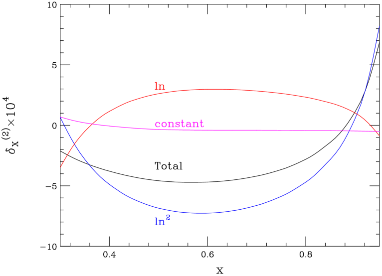
Figure 7: The ratio of the ${\rm ln}^{2}$, ${\rm ln}$, and constant NNLO coefficients, as well as the total result, relative to the tree result, $\delta^{(2)}_{X}=(\alpha/\pi)^{2}f^{(2)}_{X}(x)/f^{(0)}(x)$, versus the electron energy fraction $x$. The $y$-axis has been scaled by $10^{4}$.

An interesting feature of the electron energy spectrum is that effects of radiative corrections are enhanced by large logarithms of the ratio of the muon mass over the electron mass. The computation of the logarithmically enhanced terms in the spectrum is a much simpler problem than the full calculation reported in this paper. Since large logarithms are routinely exploited in theoretical physics for a simplified description, it is interesting to gain some experience on how well this approximation works in various calculations. To do so, we compare the double- and single-logarithmic enhanced corrections with the full second order QED correction to the electron energy spectrum in Fig. 7. We see that the ratio of the single logarithmic term over the constant term obeys the expectation $|f^{(2)}_{1}(x)/f^{(2)}_{0}(x)|\sim{\rm ln}(m_{\mu}/m_{e})\approx 5$, while the ratio of the double logarithmic term over the single logarithmic term doesn’t: $|f^{(2)}_{2}(x)/f^{(2)}_{1}(x)|<5$. Moreover, we note that the double-logarithmic terms overestimate the full correction. Because of the cancellation between the doubly- and singly-logarithmic enhanced terms, the relative importance of $f^{(2)}_{0}(x)$ increases. For example, at $x=0.5$, the constant term $f^{(2)}_{0}(x)$ changes the second order correction by about $10\%$; this should be compared with the naive estimate $1/\ln^{2}(m_{\mu}/m_{e})\sim 4\%$. From this we conclude that the leading logarithmic corrections give a correct order-of-magnitude estimate; however, the full result can deviate from the leading logarithmic approximation by a factor of $2-3$.

V Conclusions

In this paper, we have presented a calculation of the ${\cal O}(\alpha^{2})$ QED corrections to the electron energy spectrum in muon decay. The NNLO QED corrections, relative to the tree level result, are in the range $-5\,\,{\rm to}\,\,8\times 10^{-4}$, depending on the electron energy. This is larger than the $10^{-4}$ precision expected from the TWIST experiment at TRIUMF. The corrections contain logarithmically enhanced terms of the form ${\rm ln}(m_{\mu}/m_{e})$, which have been calculated previously in Arbuzov:2002pp ; Arbuzov:2002cn . The new result derived here is the constant term without logarithmic enhancement, which influences the spectrum at the level of $\sim 0.5\times 10^{-4}$. The inclusion of this correction reduces the theoretical uncertainty below the anticipated experimental precision. We have argued the the remaining uncertainty is at the level of $5\times 10^{-6}$, which is negligible for any foreseeable experiment.

Although only the electron energy spectrum is considered in this paper, the computational method introduced is flexible enough to permit a computation of any distribution in muon decay, with arbitrary restrictions on the kinematic variables of the electrons and photons. The calculation reported here can therefore be extended in several ways. For the TWIST experiment, there are two natural extensions: (1) to include polarization of the muon, which is present in the experimental setup; (2) to also constrain the lab-frame angle ${\rm cos}\,\theta$ of the electron, in order to match the fiducial region used by the TWIST experiment in their first analysis, $0.50\leq{\rm cos}\,\theta\leq 0.84$ twistik .

There are several applications of our method beyond muon decay, where precise calculations of the decay spectra of massive particles are required. Higher order corrections to semileptonic and radiative $b$ decays are needed for extraction of CKM matrix elements and fundamental parameters in heavy quark physics, and in searches for new physics. Decay distributions of top quarks, Higgs bosons, and new massive particles will be precisely measured at the LHC and at a future linear collider, and will be used to elucidate the underlying theory describing what is discovered. We anticipate that the techniques developed here will be useful in performing these analyses.

Acknowledgments. This research was supported by the US Department of Energy under contract DE-FG03-94ER-40833 and the Outstanding Junior Investigator Award DE-FG03-94ER-40833, and by the National Science Foundation under contracts P420D3620414350, P420D3620434350.

References

- (1) G. Bardin et al., Phys. Lett. B 137, 135 (1984), Nucl. Phys. A 352, 365 (1981).
- (2) G. W. Bennett et al. [Muon g-2 Collaboration], Phys. Rev. Lett. 89, 101804 (2002) [Erratum-ibid. 89, 129903 (2002)] [arXiv:hep-ex/0208001].
- (3) H. N. Brown et al. [Muon g-2 Collaboration], Phys. Rev. Lett. 86, 2227 (2001) [arXiv:hep-ex/0102017].
- (4) For a review, see A. Czarnecki and W. J. Marciano, Phys. Rev. D 64, 013014 (2001).
- (5) For a review, see Y. Kuno and Y. Okada, Rev. Mod. Phys. 73, 151 (2001).
- (6) T. Kinoshita, J. Phys. G29, 9 (2003).
- (7) R. E. Behrends, R. J. Finkelstein and A. Sirlin, Phys. Rev. 101, 866 (1956); S. M. Berman, Phys. Rev. 112, 267 (1958); T. Kinoshita and A. Sirlin, Phys. Rev. 113, 1652 (1959).
- (8) T. Kinoshita, J. Math. Phys. 3, 650 (1962); T. D. Lee and M. Nauenberg, Phys. Rev. 133, B1549 (1964).
- (9) T. W. Appelquist, J. R. Primack and H. R. Quinn, Phys. Rev. D 6, 2998 (1972).
- (10) T. van Ritbergen and R. G. Stuart, Phys. Rev. Lett. 82, 488 (1999) [arXiv:hep-ph/9808283]; T. van Ritbergen and R. G. Stuart, Nucl. Phys. B 564, 343 (2000) [arXiv:hep-ph/9904240]; M. Steinhauser and T. Seidensticker, Phys. Lett. B 467, 271 (1999) [arXiv:hep-ph/9909436].
-
(11)
M. Awramik and M. Czakon,
Phys. Lett. B 568, 48 (2003),
Phys. Rev. Lett. 89, 241801 (2002);
A. Onishchenko and O. Veretin, Phys. Lett. B 551, 111 (2003). - (12) M. Quraan et al., Nucl. Phys. A 663, 903 (2000); N. L. Rodning et al., Nucl. Phys. Proc. Suppl. 98, 247 (2001).
- (13) A. Gaponenko et al. [TWIST Collaboration], Phys. Rev. D71, 071101 (2005) [arXiv:hep-ex/0410045]; J. R. Musser [TWIST Collaboration], Phys. Rev. Lett. 94, 101805 (2005) [arXiv:hep-ex/0409063].
-
(14)
L. Michel,
Proc. Phys. Soc. A 63, 514 (1950);
C. Bouchiat and L. Michel, Phys. Rev. 106, 170 (1956). - (15) A. Arbuzov, A. Czarnecki and A. Gaponenko, Phys. Rev. D 65, 113006 (2002) [arXiv:hep-ph/0202102].
- (16) A. Arbuzov and K. Melnikov, Phys. Rev. D 66, 093003 (2002) [arXiv:hep-ph/0205172].
- (17) C. Anastasiou, K. Melnikov and F. Petriello, Phys. Rev. D 69, 076010 (2004) [arXiv:hep-ph/0311311]; C. Anastasiou, K. Melnikov and F. Petriello, Phys. Rev. Lett. 93, 032002 (2004) [arXiv:hep-ph/0402280]; C. Anastasiou, K. Melnikov and F. Petriello, arXiv:hep-ph/0409088; C. Anastasiou, K. Melnikov and F. Petriello, arXiv:hep-ph/0501130.
-
(18)
P. Gambino and N. Uraltsev, Eur. Phys. Jour. C34, 181 (2004);
C.W. Bauer et al., Phys. Rev. D67, 054012 (2003). - (19) For reviews of precision top and Higgs measurements at the LHC and ILC, see M. Beneke et al., arXiv:hep-ph/0003033; G. Weiglein et al. [LHC/LC Study Group], arXiv:hep-ph/0410364.
- (20) S. M. Berman and A. Sirlin, Ann. Phys. 20, 20 (1962).
- (21) A. B. Arbuzov, Phys. Lett. B 524, 99 (2002) [arXiv:hep-ph/0110047].
-
(22)
F. V. Tkachov, Phys. Lett. B100, 65 (1981);
K.G. Chetyrkin and F.V. Tkachov, Nucl. Phys. B192, 159 (1981). - (23) S. Laporta, Int. J. Mod. Phys. A15, 5087 (2000).
- (24) C. Anastasiou and A. Lazopoulos, JHEP 0407, 046 (2004) [arXiv:hep-ph/0404258].
- (25) T. Binoth and G. Heinrich, Nucl. Phys. B 585, 741 (2000).
- (26) T. Binoth and G. Heinrich, Nucl. Phys. B 680, 375 (2004) [arXiv:hep-ph/0305234].
- (27) N. Gray, D.J. Broadhurst, W. Grafe and K. Schilcher, Z. Phys. C48, 673 (1990); D.J. Broadhurst, N. Gray and K. Schilcher, Z. Phys. C52, 111 (1991).
- (28) K. Melnikov and T. van Ritbergen, Nucl. Phys. B 591, 515 (2000) [arXiv:hep-ph/0005131].
- (29) C. Anastasiou, E. W. N. Glover and C. Oleari, Nucl. Phys. B 575, 416 (2000) [Erratum-ibid. B 585, 763 (2000)] [arXiv:hep-ph/9912251].
- (30) O. V. Tarasov, Phys. Rev. D 54, 6479 (1996) [arXiv:hep-th/9606018].
- (31) T. van Ritbergen and R. G. Stuart, Phys. Lett. B 437, 201 (1998) [arXiv:hep-ph/9802341].
- (32) A. I. Davydychev, K. Schilcher and H. Spiesberger, Eur. Phys. J. C 19, 99 (2001) [arXiv:hep-ph/0011221].
- (33) A.B. Arbuzov, JHEP 0303, 063 (2003).