CERN-PH-TH/2005-079

SLAC-PUB-11177

Reduction of Charm Quark Mass Scheme Dependence

in $\bar{B}\rightarrow X_{s}\gamma$ at the NNLL Level

H.M. Asatrian^a, C. Greub^b, A. Hovhannisyan^a,

T. Hurth^c,d, and V. Poghosyan^a

^a Yerevan Physics Institute, 375036, Yerevan, Armenia

^b Institute for Theoretical Physics, University Berne, CH-3012 Berne, Switzerland

^c Theoretical Physics Division, CERN, CH-1211 Geneva 23, Switzerland

^d SLAC, Stanford University, Stanford, CA 94309, USA

The uncertainty of the theoretical prediction of the $\bar{B}\rightarrow X_{s}\gamma$ branching ratio at NLL level is dominated by the charm mass renormalization scheme ambiguity. In this paper we calculate those NNLL terms which are related to the renormalization of $m_{c}$, in order to get an estimate of the corresponding uncertainty at the NNLL level. We find that these terms significantly reduce (by typically a factor of two) the error on $\mbox{BR}(\bar{B}\to X_{s}\gamma)$ induced by the definition of $m_{c}$. Taking into account the experimental accuracy of around $10\%$ and the future prospects of the $B$ factories, we conclude that a NNLL calculation would increase the sensitivity of the observable $\bar{B}\rightarrow X_{s}\gamma$ to possible new degrees of freedom beyond the SM significantly.

1 Introduction

The branching ratio of $\bar{B}\rightarrow X_{s}\gamma$ is a very sensitive probe for new degrees of freedom beyond the standard model (SM) (for a review, see [1]). Within supersymmetric extensions of the SM for example, one can derive stringent bounds on the parameter space of these models [2, 3, 4, 5, 6, 7, 8]. Clearly, such bounds will be most valuable when the general nature of the new physics beyond the SM will be identified at the forthcoming LHC experiments.

Because of the heavy mass expansion that is valid for inclusive decay modes, the decay rate of $\bar{B}\rightarrow X_{s}\gamma$ is dominated by the perturbatively calculable partonic decay rate $\Gamma(b\rightarrow X_{s}\gamma$). QCD corrections to the latter, due to hard-gluon exchange, are the most important perturbative contributions; they were calculated in the past up to the next-to-leading logarithmic (NLL) level [9, 10, 11, 12, 13, 14, 15, 16, 17, 18]. Subsequently, also electroweak corrections were calculated [19, 20, 21, 22]. After completion of these computations, it was generally believed that the theoretical uncertainty of the branching ratio is below $10\%$.

However, as first pointed out in 2001 in [23], there is an additional uncertainty in the NLL results for $\Gamma(b\to X_{s}\gamma)$ which is related to the definition (renormalization scheme) of the charm quark mass. Technically, the charm quark mass depencence enters through the matrix elements $\langle s\gamma|O_{1,2}|b\rangle$ which in the context of a NLL have to be calculated up to $O(\alpha_{s})$. As these matrix elements vanish at the lowest order, the charm quark $m_{c}$ only enters (through the ratio $m_{c}/m_{b}$) at $O(\alpha_{s})$. As a consequence, the charm quark mass does not get renormalized in a NLL calculation, which means that the symbol $m_{c}$ can be identified with $m_{c,\rm{pole}}$ or with the $\overline{\mbox{MS}}$ mass $\bar{m}_{c}(\mu_{c})$ at some scale $\mu_{c}$ or with some other definition of $m_{c}$. Formally, all these assignements are equivalent, as they lead to differences which are of order $\alpha_{s}^{2}$.

Note that in contrast to the $c$-quark mass the $b$-quark mass does get renormalized in a NLL calculation and we choose to express all the following results in terms of $m_{b,\rm{pole}}$. In this respect we do not follow ref. [23], where the $m_{b,1S}$ mass was used. Unless stated otherwise, the symbol $m_{b}$ stands for $m_{b,\rm{pole}}$ in all the formulas in this paper. Numerically, we use $m_{b}=4.8$ GeV throughout.

Numerically, it turns out that the NLL result for $\Gamma(b\to X_{s}\gamma)$ strongly depends on which mass definition of the charm quark mass is used in the NLL expressions. To illustrate this, we first identify $m_{c}$ with $m_{c,\rm{pole}}$ as it was done in all analyses before the paper of Gambino and Misiak [23]. Numerically, we use $m_{c,\rm{pole}}/m_{b,\rm{pole}}=0.29$ which is based on the mass difference $m_{b,\rm{pole}}-m_{c,\rm{pole}}=3.4$ GeV fixed through the heavy mass expansion of $m_{B}$ and $m_{D}$ and $m_{b,\rm{pole}}=4.8$ GeV. The corresponding branching ratio then reads [23]

$$\mbox{BR}[\bar{B}\to X_{s}\gamma]_{E_{\gamma}>m_{b}/20} = 3.35\times 10^{-4}\,.$$ (1)

As the charm quarks which are propagating in a loop have a typical virtuality of $m_{b}/2$, the authors of Ref. [23] suggested to use $\bar{m}_{c}(\mu_{c})$ with $\mu_{c}\in[m_{c},m_{b}]$ instead of $m_{c,\rm{pole}}$. A typical value for the corresponding ratio is $\bar{m}_{c}(\mu_{c})/m_{b,\rm{pole}}=0.22$. Using this value, the branching ratio gets increased w.r.t. (1) by about $11\%$ [23]:

$$\mbox{BR}[\bar{B}\to X_{s}\gamma]_{E_{\gamma}>m_{b}/20} = 3.73\times 10^{-4}\,.$$ (2)

In a recent theoretical update of the NLL prediction of this branching ratio, the uncertainty related to the definition of $m_{c}$ was taken into account by varying $m_{c}/m_{b}$ in the conservative range $0.18\leq m_{c}/m_{b}\leq 0.31$ which covers both, the pole mass (with its numerical error) value and the running mass $\bar{m}_{c}(\mu_{c})$ value with $\mu_{c}\in[m_{c},m_{b}]$ [24]:

$$\mbox{BR}[\bar{B}\to X_{s}\gamma]=(3.70\pm 0.35|_{m_{c}/m_{b}}\pm 0.02|_{\rm{CKM}}\pm 0.25|_{\rm{param.}}\pm 0.15|_{\rm{scale}})\times 10^{-4}\,.$$ (3)

There exists a large number of measurements of the inclusive decay $\bar{B}\rightarrow X_{s}\gamma$ [25, 26, 27, 28, 29, 30] and the present experimental accuracy has reached the $10\%$ level [31]:

$$\mbox{BR}[\bar{B}\to X_{s}\gamma]=(3.52\pm 0.30)\times 10^{-4}\,.$$ (4)

In the near future, more precise data on this mode are expected from the $B$ factories. Thus, it is mandatory to reduce the present theoretical uncertainty accordingly. A systematic improvement certainly consists in performing a complete NNLL calculation . This is, however, a very complicated task (for discussion and some results see [32, 33, 34, 35]) and a certain motivation is needed to enter such an enterprise. In the present paper we try to give such a motivation: By calculating those NNLL terms which are induced by renormalizing the charm quark mass in the NLL expressions, i.e. those terms which are sensitive to the definition of the charm quark mass, we show that the large error at the NLL level related to the $m_{c}$ definition gets significantly reduced. As this error is the dominant one at the NLL level (see eq. (3)), we conclude that a complete NNLL calculation will drastically improve the theoretical prediction of the branching ratio. We stress here that in the present paper we only make a statement about the reduction of the error at the NNLL level, and not about the central value of the branching ratio; this remains the topic of a complete NNLL calculation!

The remainder of this paper is organized as follows. In section 2 we discuss in some detail how to calculate the NNLL terms induced by renormalizing $m_{c}$ in the NLL results. In order to make the paper self-contained, we first list in section 3 the structure of the NNL results and then we present the analytical results for the new terms discussed in section 2. Finally, in section 4, we numerically investigate by how much the error related to the definition of $m_{c}$ gets reduced at the NNLL level.

2 NNLL terms related to $m_{c}$ renormalization

As already explained in the introduction, the matrix elements $M_{1,2}^{\rm{virt}}(m_{c})=\langle s\gamma|O_{1,2}(\mu_{b})|b\rangle$ only start at order $O(\alpha_{s}^{1})$, or, in other words at the NLL order. As a consequence, the definition of $m_{c}$ is not fixed at this order, because $m_{c}$ does not get renormalized. This is also true for the bremsstrahlung contributions $M_{1,2}^{\rm{brems}}(m_{c})=\langle s\gamma g|O_{1,2}(\mu_{b})|b\rangle$, which are needed up to $O(g_{s})$ for a NLL calculation. In this section we concentrate on the virtual terms $M_{1,2}^{\rm{virt}}(m_{c})$, as the extension to the bremsstrahlung contributions $M_{1,2}^{\rm{brems}}(m_{c})$ is straightforward.

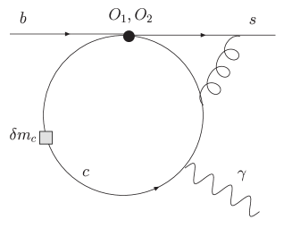
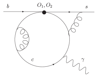
Figure 1: Left frame: Typical $\delta m_{c}$ insertion diagram (see text). Right frame: Typical diagram with a charm quark self-energy insertion (see text).

When going to NNLL precision, the matrix elements $M_{1,2}^{\rm{virt}}(m_{c})$ are needed to $O(\alpha_{s}^{2})$. At this level, there are – among many other diagrams – counterterm contributions to these matrix elements, induced by the renormalization of $m_{c}$ (see the left frame of Fig. 1). The complete set of such diagrams is generated by inserting the operator $-i\delta m_{c}\bar{\psi}_{c}\,\psi_{c}$ in the $O(\alpha_{s})$ diagrams of $O_{1,2}$ in all possible ways. The sum $\delta M^{\rm{virt}(\epsilon)}_{1,2}(m_{c})\cdot\delta m_{c}$ of all these insertions can be obtained by replacing $m_{c}\to m_{c}+\delta m_{c}$ in the $O(\alpha_{s}^{1})$ results $M^{\rm{virt}(\epsilon)}_{1,2}(m_{c})$, followed by expanding in $\delta m_{c}$ up to linear order:

$$M_{1,2}^{\rm{virt}(\epsilon)}(m_{c}+\delta m_{c})=M_{1,2}^{\rm{virt}(\epsilon)}(m_{c})+\delta M^{\rm{virt}(\epsilon)}_{1,2}(m_{c})\cdot\delta m_{c}+O((\delta m_{c})^{2})\,.$$ (5)

As $\delta m_{c}$ is ultraviolet divergent, the matrix elements $M_{1,2}^{\rm{virt}(\epsilon)}(m_{c})$ are needed in our application up to order $\epsilon^{1}$, as indicated by the notation in eq. (5).

The explicit shift $\delta m_{c}$ depends of course on the renormalization scheme. When aiming at expressing the results for $M_{1,2}^{\rm{virt}(\epsilon)}(m_{c})$ in terms of $\bar{m}_{c}(\mu_{b})$, the shift reads ($C_{F}=4/3$)

$$\delta\bar{m}_{c}(\mu_{b}) = -\frac{\alpha_{s}(\mu_{b})}{4\pi}\,C_{F}\,\frac{3}{\epsilon}\,\bar{m}_{c}(\mu_{b})\,.$$

On the other hand, when the result is expressed in terms of $m_{c,\rm{pole}}$, the shift reads

$$\delta m_{c,\rm{pole}} = -\frac{\alpha_{s}(\mu_{b})}{4\pi}\,C_{F}\,\left(\frac{3}{\epsilon}+3\ln\frac{\mu_{b}^{2}}{m_{c}^{2}}+4\right)\,m_{c,\rm{pole}}\,.$$

The infinities induced by the $1/\epsilon$ terms in $\delta m_{c}$ get cancelled in a full NNLL calculation, in particular by self-energy diagrams depicted in the right frame of Fig. 1. As we do not perform a full NNLL calculation, we suggest to consider self-energy insertions, where the self-energy $\Sigma(p^{2})$ is replaced by $\Sigma_{1}(p^{2}=m_{c}^{2})$.

The $\Sigma_{1}$-part of the self-energy $\Sigma_{1}(p^{2})$ is defined through the decomposition of the full unrenormalized self-energy $\Sigma(p^{2})$ as

$$\Sigma(p^{2})\equiv\Sigma_{2}(p^{2})(/p-m_{c})+\Sigma_{1}(p^{2}).$$ (6)

At the one-loop level, the corresponding pieces $\Sigma_{1}^{R}$ and $\Sigma_{2}^{R}$ of the renormalized self-energy are

$$\Sigma_{2}^{R}(p^{2})=\Sigma_{2}(p^{2})+\delta Z_{c},\quad\quad\Sigma_{1}^{R}(p^{2})=\Sigma_{1}(p^{2})+\delta m_{c}\,,$$ (7)

where $Z_{c}=1+\delta Z_{c}$ denotes the wave function renormalization constant of the charm quark. Eq. (7) implies that the sigularities in $\delta M_{1,2}^{\rm{virt}(\epsilon)}(m_{c})\cdot\delta m_{c}$ cancel when combined with the diagrams with $\Sigma_{1}(p^{2})$ insertions. However, for general $p^{2}$, the function $\Sigma_{1}(p^{2})$ depends on the gauge parameter $\xi$:

$$\Sigma_{1}(p^{2})=\frac{\alpha_{s}(\mu_{b})}{4\pi}C_{F}m_{c}\left\{3\left[\frac{1}{\epsilon}+\ln\frac{\mu_{b}^{2}}{m_{c}^{2}}\right]+4+\left(1-\frac{m_{c}^{2}}{p^{2}}\right)\left[\xi-\left(3-\xi\frac{m_{c}^{2}}{p^{2}}\right)\ln\left(1-\frac{p^{2}}{m_{c}^{2}}\right)\right]\right\}\,.$$

As for $p^{2}=m_{c}^{2}$ the self-energy piece $\Sigma_{1}(p^{2}=m_{c}^{2})$ is gauge-independent, we add $\Sigma_{1}(p^{2}=m_{c}^{2})$ insertions to $\delta M_{1,2}^{\rm{virt}(\epsilon)}(m_{c})\cdot\delta m_{c}$.

These momentum independent $\Sigma_{1}(p^{2}=m_{c}^{2})$ insertions can be straightforwardly aborbed into $\delta m_{c}^{\rm{eff}}$ insertions:

$$\delta m_{c,\rm{pole}}^{\rm{eff}} = \Sigma_{1}(p^{2}=m_{c}^{2})+\delta m_{c,\rm{pole}}=0\,,$$ (8)

$$\delta\bar{m}_{c}^{\rm{eff}}(\mu_{b}) = \Sigma_{1}(p^{2}=m_{c}^{2})+\delta\bar{m}_{c}(\mu_{b})=\frac{\alpha_{s}(\mu_{b})}{4\pi}\,C_{F}\,\left(3\ln\frac{\mu_{b}^{2}}{m_{c}^{2}}+4\right)\,\bar{m}_{c}(\mu_{b})\,.$$

Finally, if we wish to express the matrix elements $M^{\rm{virt}(\epsilon)}_{1,2}(m_{c})$ in terms of $\bar{m}_{c}(\mu_{c})$, the shift reads

$$\delta\bar{m}_{c}^{\rm{eff}}(\mu_{c})=\frac{\alpha_{s}(\mu_{b})}{4\pi}\,C_{F}\,\left(3\ln\frac{\mu_{c}^{2}}{m_{c}^{2}}+4\right)\,\bar{m}_{c}(\mu_{c})\,.$$ (9)

3 Analytical results

Before turning to the contributions induced through the renormalization of the charm quark mass, which are NNLL terms, we first summarize the structure of the NLL result for the branching ratio for $b\to X_{s}\gamma$. We write the decay width for $b\to X_{s}\gamma$ using a photon energy cut $E_{0}=\frac{m_{b}}{2}(1-\delta)=E_{max}(1-\delta)$ as

$$\Gamma(b\to X_{s}\gamma)_{E_{\gamma}\geq E_{0}}=\Gamma(b\to s\gamma)+\Gamma(b\to s\gamma g)_{E_{\gamma}\geq E_{0}}\,,$$ (10)

where the two parts are defined as follows:

$$\Gamma(b\to s\gamma)=\frac{G_{F}^{2}}{32\pi^{4}}|V_{ts}^{*}V_{tb}|^{2}\alpha_{em}m_{b,\rm{pole}}^{5}\,|D|^{2},$$

$$\Gamma(b\to s\gamma g)_{E_{\gamma}\geq E_{0}}=\frac{G_{F}^{2}}{32\pi^{4}}|V_{ts}^{*}V_{tb}|^{2}\alpha_{em}m_{b,\rm{pole}}^{5}\,A,$$

$$D=C_{7}^{(0)\rm{eff}}(\mu_{b})+\frac{\alpha_{s}(\mu_{b})}{4\pi}\left(C_{7}^{(1)\rm{eff}}(\mu_{b})+\sum_{i=1}^{8}C_{i}^{(0)\rm{eff}}(\mu_{b})\left[r_{i}+\gamma_{i7}^{(0)\rm{eff}}\ln\left(\frac{m_{b}}{\mu_{b}}\right)\right]-\frac{16}{3}C_{7}^{(0)\rm{eff}}(\mu_{b})\right),$$

$$A=\left(e^{-\alpha_{s}(\mu_{b})\ln(\delta)[7+2\ln(\delta)]/(3\pi)}-1\right)|C_{7}^{(0)\rm{eff}}(\mu_{b})|^{2}+\frac{\alpha_{s}(\mu_{b})}{\pi}\sum_{i,j=1,i\leq j}^{8}C_{i}^{(0)\rm{eff}}(\mu_{b})C_{j}^{(0)\rm{eff}}(\mu_{b})f_{ij}(\delta)\,.$$

The expressions for the Wilson coefficients $C_{i}(\mu_{b})$ can be found in [36]. Their numerical values we take from table 5.1 in ref. [37]. Writing the results in this specific form, the functions $f_{ij}(\delta)$ and $r_{i}$ are understood to be taken from [11] and not from the original paper [10] where the results were parametrized differently.

Following common practice, we write the branching ratio (without taking into account non-perturbative corrections) as

$$BR(b\to X_{s}\gamma)_{E_{\gamma}\geq E_{0}}=\frac{\Gamma(b\to X_{s}\gamma)_{E_{\gamma}\geq E_{0}}}{\Gamma(b\to X_{c}e\bar{\nu})}\,\mbox{BR}_{sl}^{exp}\,,$$ (13)

where the semileptonic decay rate is given by

$$\Gamma(b\to X_{c}e^{-}\bar{\nu})=\frac{G_{F}^{2}\,m_{b,\rm{pole}}^{5}}{192\pi^{3}}\,|V_{cb}|^{2}\,g\!\left(\frac{m_{c}^{2}}{m_{b}^{2}}\right)\,K\!\left(\frac{m_{c}^{2}}{m_{b}^{2}}\right)\,.$$ (14)

$g(z)=1-8\,z+8\,z^{3}-z^{4}-12\,z^{2}\,\ln(z)\,$ is the phase-space factor and the function

$$K(z)=1-\frac{2\alpha_{s}(m_{b})}{3\pi}\,\frac{f(z)}{g(z)},$$

with

$$f(z)=-(1-z^{2})\,\left(\frac{25}{4}-\frac{239}{3}\,z+\frac{25}{4}\,z^{2}\right)+z\,\ln(z)\left(20+90\,z-\frac{4}{3}\,z^{2}+\frac{17}{3}\,z^{3}\right)$$

$$+z^{2}\,\ln^{2}(z)\,(36+z^{2})+(1-z^{2})\,\left(\frac{17}{3}-\frac{64}{3}\,z+\frac{17}{3}\,z^{2}\right)\,\ln(1-z)$$

$$-4\,(1+30\,z^{2}+z^{4})\,\ln(z)\ln(1-z)-(1+16\,z^{2}+z^{4})\left(6\,\mbox{Li}(z)-\pi^{2}\right)$$

$$-32\,z^{3/2}(1+z)\left[\pi^{2}-4\,\mbox{Li}(\sqrt{z})+4\,\mbox{Li}(-\sqrt{z})-2\ln(z)\,\ln\left(\frac{1-\sqrt{z}}{1+\sqrt{z}}\right)\right]\,.$$

accounts for $O(\alpha_{s})$ QCD corrections. We note that $m_{c}$ is understood to be the pole mass in eq. (14).

We now turn to that part of NNLL corrections which is responsible for the reduction of the charm quark mass renormalization scheme dependence, as explained in section 2. We first turn to terms $\delta M_{1,2}^{\rm{virt}(\epsilon)}$ induced by $m_{c}$ renormalization in the matrix elements $M_{1,2}^{\rm{virt}(\epsilon)}$. To this end, we need $M_{1,2}^{\rm{virt}(\epsilon)}$ up to oder $\epsilon^{1}$. In [10] have calculated these matrix elements up to terms $\epsilon^{0}$, using Mellin-Barnes representations for generalized propogator to obtain analytic results in the form of the series in $z=\left(m_{c}/m_{b}\right)^{2}$ and $L=\ln(z)$. As in these calculations the expansion in $\epsilon$ was the last step, it is straightforward to calculate $M_{1,2}^{\rm{virt}(\epsilon)}$ up to order $\epsilon^{1}$.

In order to get finite results for these matrix elements, we add counterterms related to operator mixing as in ref. [10], adapted however, to the operator basis defined in ref. [11]. This step leads to $M_{1,2}^{\rm{virt,ren}}$, which we decompose as in ref. [10]:

$$M_{2}^{\rm{virt,ren}}=\langle s\gamma|O_{7}|b\rangle\,\frac{\alpha_{s}}{4\pi}\left(\frac{416}{81}\ln\frac{m_{b}}{\mu_{b}}-\frac{784}{81}\epsilon\ln^{2}\frac{m_{b}}{\mu_{b}}-4\epsilon\ln\frac{m_{b}}{\mu_{b}}r_{2}^{(0)}+r_{2}^{(0)}+r_{2}^{(1)}\epsilon\right)\,.$$ (15)

We obtain for $r_{2}=r_{2}^{(0)}+\epsilon r_{2}^{(1)}$ (note that $r_{1}=-\frac{1}{6}\,r_{2}$):

$$r_{2}^{(0)} = -{\frac{1666}{243}}-{\frac{8}{27}}\left(-48-3\,{L}^{2}-{L}^{3}+5\,{\pi}^{2}+9\,L\,(-4+{\pi}^{2})+36\,\zeta(3)\right)z+{\frac{32}{27}}\,{\pi}^{2}{z}^{3/2}$$

$$+{\frac{8}{27}}\,\left({L}^{3}-6\,L(-2+{\pi}^{2})+18+2\,{\pi}^{2}\right){z}^{2}-{\frac{4}{81}}\,\left(9-182\,L+126\,{L}^{2}+14\,{\pi}^{2}\right){z}^{3}$$

$$-\frac{8\,i\,\pi}{27}\left[{\frac{10}{3}}+2\,\left(-15-3\,L-3\,{L}^{2}+{\pi}^{2}\right)z+2\,\left(-3\,{L}^{2}+{\pi}^{2}\right){z}^{2}+{\frac{8}{3}}\,\left(-7+3\,L\right)\,{z}^{3}\right]$$

$$r_{2}^{(1)} = -{\frac{19577}{729}}+{\frac{184}{243}}\,{\pi}^{2}-{\frac{2}{405}}\left(-18180+75\,{L}^{4}+3240\,{\pi}^{2}+46\,{\pi}^{4}-30\,{L}^{2}(-24+7\,{\pi}^{2})\right.$$ (17)

$$\left.+9000\,\zeta(3)+120\,L(-66+14\,{\pi}^{2}+27\,\zeta(3))\right)z-{\frac{32}{81}}\,{\pi}^{2}\left(-49+6\,L+24\,\ln(2)\right){z}^{3/2}$$

$$+{\frac{2}{81}}\left(48\,{L}^{3}-15\,{L}^{4}+24\,{L}^{2}(-3+{\pi}^{2})-24\,L(3+5\,{\pi}^{2})+1116+36\,{\pi}^{2}\right.$$

$$\left.+40\,{\pi}^{4}+432\,\zeta(3)\right){z}^{2}-{\frac{1120}{81}}\,{\pi}^{2}{z}^{5/2}+{\frac{1}{729}}\left(22705-2484\,{L}^{2}+4536\,{L}^{3}-6036\,{\pi}^{2}\right.$$

$$\left.+6\,L(-1783+192\,{\pi}^{2})+8208\,\zeta(3)\right){z}^{3}$$

$$+{\frac{8\,i\,\pi}{27}}\,\left[-{\frac{221}{9}}+\left(15\,{L}^{2}-6\,{L}^{3}-4\,L(-9+{\pi}^{2})+186-10\,{\pi}^{2}-36\,\zeta(3)\right)z\right.$$

$$-2\left(-3-6\,{L}^{2}+3\,{L}^{3}+2\,{\pi}^{2}+2\,L{\pi}^{2}+18\,\zeta(3)\right){z}^{2}$$

$$\left.+\frac{4}{9}\,(-67+66\,L+9\,{L}^{2}+12\,{\pi}^{2}){z}^{3}\right]$$

In these formulas we retained all terms up to order $z^{3}$, as higher order terms contribute much less than $1\%$. Nevertheless, in the numerical evaluations in section 4 all terms up to $z^{6}$ were included.

At the level of the decay width, the implementation of the contribution coming from renormalization of the $c$-quark mass in the virtual contributions is (according to eq. (5)) most easily achieved by replacing $r_{1,2}$ in eq. (3) by $r_{1,2}^{(0)}+\Delta r_{1,2}$, where

$$\Delta r_{1,2}=\delta m_{c}\frac{d}{dm_{c}}\left(r_{1,2}^{(0)}+\epsilon\,r_{1,2}^{(1)}\right)\,.$$ (18)

At the NLL order, the bremsstrahlung corrections to the decay width are encoded in the quantities $f_{ij}(\delta)$ (see eq. (3)), which correspond to the interference terms $(O_{i},O_{j})$. In the following, we calculate the shifts $\Delta f_{ij}$ to these quantities induced by the renormalization of the charm quark mass. In principle, we calculate the decay width using a photon energy cut $\delta=0.9$ (see eq. (10)). However, as all bremsstrahlung contributions which contain charm quark loops are finite for $\delta\to 1$, we can approximate these terms by putting $\delta=1$. Numerically the relative error is of order $10^{-4}$.

We first calculate the shift $\Delta f_{27}$. To this end, we shift the charm quark mass in the matrix element of $\langle s\gamma g|O_{2}|b\rangle$ as in eq. (5) and then work out the interference with $\langle s\gamma g|O_{7}|b\rangle$. Because of the $1/\epsilon$ term in $\delta m_{c}$, the result is ultraviolet singular. In a full NNLL calculation this singularity gets cancelled when combined with self-energy insertions in the charm quark lines in the matrix element of $O_{2}$. We therefore do the phase space integrations involved in the derivation of $f_{27}$ (or $\Delta f_{27}$) in d=4 dimensions. As only the matrix element of $O_{2}$ depends on $m_{c}$, the shift $\Delta f_{27}$ can be constructed by first considering the quantity $f_{27}$ itself. Using the integral representation for the building block for photon and gluon emission from the $c$-quark loop [10], one obtains after integration over all but one of the phase space parameters

$$f_{27}=-\frac{8}{9}\left(\frac{\mu_{b}}{m_{b}}\right)^{2\epsilon}\int dx\,dy\,du\,u^{2}(1-u)(1-x)y\,\frac{[x(1-x)]^{-\epsilon}\,\Gamma(2+\epsilon)\,\mbox{e}^{\epsilon\gamma+i\epsilon\pi}}{\left[uy-\frac{z}{x(1-x)}+i\eta\right]^{(1+\epsilon)}}\,.$$ (19)

Here $x,y$ are Feynman parameters and $u$ is the remaining phase space parameter, $0\leq x,y,u\leq 1$. To solve the integrals, we use the Mellin–Barnes representation for the generalized propagator

$$\left[uy-\frac{z}{x(1-x)}+i\eta\right]^{-1-\epsilon} = \frac{1}{2i\pi\Gamma(1+\epsilon)}\int_{\gamma}ds\frac{\mbox{e}^{i\pi s}\,\Gamma(-s)\,\Gamma(1+\epsilon+s)}{(uy)^{1+\epsilon}}\left[\frac{z}{uyx(1-x)}\right]^{s}$$

appearing in eq. (19). $\gamma$ denotes the integration path parallel to imaginary axes which hits the real axes somewhere between $(-1-\epsilon)$ and $0$. Closing the integration path in the right $s$-half plane, one gets an expansion for $f_{27}$ in $z=(m_{c}/m_{b})^{2}$ and $L=\ln(z)$.

The shift $\Delta f_{27}$ is then obained as

$$\Delta f_{27}=\delta m_{c}\,\frac{dz}{dm_{c}}\,\frac{df_{27}}{dz}=2\frac{m_{c}}{m_{b}}\frac{\delta m_{c}}{m_{b}}\left(f_{27}^{d(0)}+\epsilon\,f_{27}^{d(1)}\right)\,.$$ (20)

To summarize, the NNLL contributions due to renormalization of $m_{c}$ in the $(O_{2},O_{7})$ interference are taken into account by replacing $f_{27}\to f_{27}^{(0)}+\Delta f_{27}$ in eq. (3). Explicitly, we find:

$$f_{27}^{(0)} = -\frac{8}{9}\left[\frac{1}{12}+\frac{1}{8}(7-2\pi^{2}+6L+2L^{2})z+(\pi^{2}-2L-L^{2})z^{2}\right.$$

$$+ \left.\frac{1}{4}(-11-6\pi^{2}-4L+6L^{2})z^{3}+\frac{1}{3}(-6+10L)z^{4}\right.$$

$$+ \left.\frac{1}{24}(13+70L)z^{5}+\frac{1}{15}(32+63L)z^{6}\right]\,,$$

$$f_{27}^{d(0)} = -\frac{8}{9}\left[\frac{1}{8}(13-2\pi^{2}+10L+2L^{2})+2(-1+\pi^{2}-3L-L^{2})z\right.$$

$$+ \left.\frac{1}{4}(-37-18\pi^{2}+18L^{2})z^{2}+\frac{2}{3}(-7+20L)z^{3}\right.$$

$$+ \left.\frac{5}{24}(27+70L)z^{4}+\frac{1}{5}(85+126L)z^{5}\right]\,,$$

$$f_{27}^{d(1)} = -\frac{8}{9}\left[\frac{1}{48}(165-52\pi^{2}-4(-15+\pi^{2})L-18L^{2}-8L^{3}-72\zeta(3))\right.$$

$$+ \left.\frac{1}{3}(2(-12+\pi^{2})L-3L^{2}+4L^{3}+6(-5+4\pi^{2}+6\zeta(3)))z\right.$$

$$- \left.\frac{3}{4}(-7+15\pi^{2}+(15+2\pi^{2})L-15L^{2}+4L^{3}+36\zeta(3))z^{2}\right.$$

$$- \left.\frac{5}{27}(235+48\pi^{2}-204L+36L^{2})z^{3}\right.$$

$$+ \left.\frac{1}{432}(-10076-4200\pi^{2}+19425L-3150L^{2})z^{4}\right.$$

$$+ \left.\frac{1}{250}(-3554-4200\pi^{2}+20685L-3150L^{2})z^{5}\right]\,.$$

Note that $f_{27}^{0}$ in eq. (3) is an expanded version in $z$ of the integral expression for $f_{27}$ in ref. [11]. We further note that $f_{28}=-\frac{1}{3}f_{27}$, $f_{17}=-\frac{1}{6}f_{27}$, $f_{18}=\frac{1}{18}f_{27}$; the same relations also hold for the respective $\Delta f_{ij}$ (see for instance, [38]).

Finally, we turn to the shift $\Delta f_{22}$ related to the $(O_{2},O_{2})$-interference. To derive this quantity, one has to perform the shift $m_{c}\to m_{c}+\delta m_{c}$ only in one of the two interfering one-loop amplitudes $M_{2}^{\rm{brems}}=\langle s\gamma g|O_{2}|b\rangle$. To this end, one writes integral representations for both, $M_{2}^{\rm{brems}}$ and $dM_{2}^{\rm{brems}}/dm_{c}$. $\Delta f_{22}$ is then represented as a five dimensional integral (4 Feynman parameters and one phase space parameter), which can be solved by double Mellin-Barnes techniques (see for instance [39]). Omitting the detail of this calculation, the terms induced by renormalizing $m_{c}$ in the $(O_{2},O_{2})$ bremsstrahlung terms are implemented in eq. (3) by replacing $f_{22}\to f_{22}^{(0)}+\Delta f_{22}$, where

$$\Delta f_{22}=2\frac{m_{c}}{m_{b}}\frac{\delta m_{c}}{m_{b}}\left(f_{22}^{d(0)}+\epsilon\,f_{22}^{d(1)}\right)\,.$$ (24)

Explicity, we get:

$$f_{22}^{(0)} = 0.04938272+(16.64197+1.887290L-0.4444444L^{2}-0.09876543L^{3})z$$

$$+ (57.92026+47.67037L+1.185185L^{2}+3.134737L^{3}+0.05925926L^{5})z^{2}$$

$$+ (-93.12628+32.36078L-12.95977L^{2}+1.777778L^{3}-0.2962963L^{4})z^{3}$$

$$+ (11.92082-11.21491L+2.074074L^{2}-0.5925926L^{3})z^{4}$$

$$+ (0.6482797-4.160089L+0.1810700L^{2}-0.3292181L^{3})z^{5}$$

$$+ (-1.125313-4.320604L-0.2444444L^{2}-0.3456790L^{3})z^{6}\,,$$

$$f_{22}^{d(0)} = 18.52926+0.9984013L-0.7407407L^{2}-0.09876543L^{3}$$

$$+ (163.5109+97.71112L+11.77458L^{2}+6.269473L^{3}+0.2962963L^{4}+0.1185185L^{5})z$$

$$+ (-247.0180+71.16280L-33.54596L^{2}+4.148148L^{3}-0.8888889L^{4})z^{2}$$

$$+ (36.46839-40.71149L+6.518519L^{2}-2.370370L^{3})z^{3}$$

$$+ (-0.9186906-20.43831L-0.08230453L^{2}-1.646091L^{3})z^{4}$$

$$+ (-11.07248-26.41251L-2.503704L^{2}-2.074074L^{3})z^{5}\,,$$

$$f_{22}^{d(1)} = 41.24600-7.794263L-0.7525535L^{2}+0.3950617L^{3}+0.07407407L^{4}$$

$$+ (234.4505+44.95451L-64.68047L^{2}-0.5200208L^{3}$$

$$- 4.498135L^{4}-0.05925926L^{5}-0.08559671L^{6})z$$

$$+ (-368.8104+245.2526L-95.81857L^{2}+28.84099L^{3}-3.851852L^{4}+0.5728395L^{5})z^{2}$$

$$+ (-3.708986-93.16023L+34.50854L^{2}-7.670782L^{3}+1.283951L^{4})z^{3}$$

$$+ (-45.10910-54.73258L+13.39517L^{2}-4.073160L^{3}+0.8779150L^{4})z^{4}$$

$$+ (-92.60340-74.33726L+10.32328L^{2}-4.786008L^{3}+1.094650L^{4})z^{5}\,.$$

We decided to give the expansion coefficients in these equations in numerical form, because the exact results are somewhat lenghty. We note that $f_{22}^{0}$ in eq. (3) is an expanded version in $z$ of the integral expression for $f_{22}$ in ref. [11]. We further note that $f_{11}=\frac{1}{36}f_{22}$ and $f_{12}=-\frac{1}{3}f_{22}$; the same relations also hold for the respective $\Delta f_{ij}$.

These analytical results are defined parts of the complete NNLL contribution which can be used within a future NNLL calculation.

4 Numerical results

In the following analysis we show that the NNLL terms, induced through the renormalization of $m_{c}$, drastically reduce the error related to the definition of the charm quark mass in $\mbox{BR}(b\to X_{s}\gamma)$. To illustrate this feature as clearly as possible, we take the fixed values shown in Table 1 for the input parameters.

$m_{b}=4.8$ GeV

$m_{c,\rm{pole}}/m_{b}=0.29$

$m_{Z}=91.187$ GeV

$\alpha_{s}(m_{Z})={0.119}$

$\alpha_{\rm em}=1/137.036$

$|V^{*}_{ts}V_{tb}/V_{cb}|^{2}=0.95$

$BR_{\rm{sl}}=10.49\%$

Table 1: Input parameters used in the numerical analysis.

In particular, we use the fixed ratio $m_{c,\rm{pole}}/m_{b,\rm{pole}}=0.29$. Furthermore, we always leave the semileptonic decay width, which enters the branching ratio for $b\to X_{s}\gamma$ through eq. (13), expressed in terms of $m_{c,\rm{pole}}$ as given in eq. (14). In this way the $m_{c}$ definition dependence of the $\mbox{BR}(b\to X_{s}\gamma)$ only comes from the numerator in eq. (13). For our studies, we neglect electroweak corrections and non-perturbative effects. As already mentioned, in the bremsstrahlung contribution we use $\delta=0.9$ for the lower cut in the photon energy (see eq. (10)).

Starting from $m_{c,\rm{pole}}=0.29\cdot 4.8$ GeV = 1.392 GeV, we first calculate $\bar{m}_{c}(m_{c,\rm{pole}})$, using the one-loop expression

$$\bar{m}_{c}(m_{c,\rm{pole}})=m_{c,\rm{pole}}\left[1-\frac{\alpha_{s}(m_{c,\rm{pole}})}{\pi}\,C_{F}\,\right]\,.$$ (28)

To get $\bar{m}_{c}(\mu_{c})$ for an arbitrary scale (typically between 1.25 GeV and 5 GeV), we use two-loop running (with 5 flavours) according to

$$\bar{m}_{c}(\mu_{c})=\bar{m}_{c}(\mu_{0})\left(\frac{\alpha_{s}(\mu_{c})}{\alpha_{s}(\mu_{0})}\right)^{\frac{\gamma_{m}^{(0)}}{2\beta_{0}}}\left[1+\left(\frac{\gamma_{m}^{(1)}}{2\beta_{0}}-\frac{\beta_{1}\gamma_{m}^{(0)}}{2\beta_{0}^{2}}\right)\,\frac{\alpha_{s}{(\mu_{c})}-\alpha_{s}(\mu_{0})}{4\pi}\right]$$ (29)

with $\mu_{0}=m_{c,\rm{pole}}$. Numerically, we get the values shown in table 2.

$\bar{m}_{c}(1.25)/m_{b}=0.257$

$\bar{m}_{c}(2.5)/m_{b}=0.214$

$\bar{m}_{c}(5.0)/m_{b}=0.187$

Table 2: $\bar{m}_{c}(\mu_{c})/m_{b}$ for $\mu_{c}=1.25,2.5,5$ GeV using $m_{c,\rm{pole}}/m_{b}=0.29$ as input.

In Figure 2 our results are given for three different values of $\mu_{b}$, where $\mu_{b}$ represents the usual renormalization scale of the effective field theory. We compare the branching ratio for $b\to X_{s}\gamma$ within the pole and the $\overline{\rm{MS}}$ scheme for the charm quark mass. Within each vertical string the solid dot represents the branching ratio using $m_{c,\rm{pole}}$, while the open symbols correspond to $\bar{m}_{c}(\mu_{c})$ for $\mu_{c}=1.25$ GeV (triangle), $\mu_{c}=2.5$ GeV (quadrangle) and $\mu_{c}=5.0$ GeV (pentagon), respectively.

Figure 2: $\mbox{BR}(b\to X_{s}\gamma)$ for three values of $\mu_{b}$. For each value of $\mu_{b}$ the left string shows the NLL results for $m_{c,pole}$ (solid dot) and for $\bar{m}_{c}(\mu_{c})$ with $\mu_{c}=1.25;2.5;5.0$ GeV (open symbols). The right strings show the corresponding NLL results supplemented by the $\delta m_{c}$ mass insertions and the $\Sigma_{1}(p^{2}=m_{c}^{2})$ insertions (see text for more details).

For each $\mu_{b}$ the left string shows the value of the branching ratio at the NLL level, while the right string shows the corresponding value where in addition $\delta m_{c}$ mass insertions and $\Sigma_{1}(p^{2}=m_{c}^{2})$ insertions were taken into account, as explained in detail in section 2. Because the combination of these insertions is zero by construction for the pole scheme (see eq. (8)), the solid dots are at the same place in the left and the right string for a given value of $\mu_{b}$.

From Figure 2 we see that the error related to the charm quark mass definition gets significantly reduced when taking into account NNLL terms connected with mass insertions. Taking as an example the results for $\mu_{b}=5$ GeV, we find that at the NLL level the branching ratio evaluated for $\bar{m}_{c}(2.5\ \mbox{GeV})$ is $12.6\%$ higher than the one based on $m_{c,\rm{pole}}$, in agreement with ref. [23]. Including the new contributions, these $12.6\%$ get reduced to $5.1\%$.

A remark concerning the remaining NNLL terms is in order: As these terms give contributions to the branching ratio which (up to terms of order $\alpha_{s}^{3}$) do not depend on charm quark mass definition, the error related to $m_{c}$ in the full NNLL result is expected to stay essentially the same as estimated in the present paper.

However, to obtain a NNLL prediction for the central value of the branching ratio, it is of course necessary to calculate all NNLL terms.

Summing up, we have shown that the relatively large error related to the definition of the charm quark mass in the NLL result for $\mbox{BR}(b\to X_{s}\gamma)$ gets significantly reduced (typically by a factor of 2) at the NNLL level. Taking into account the present experimental accuracy of around $10\%$ and the future prospects of the $B$ factories and also of possible Super-$B$ factories [40, 41], we conclude that a future NNLL QCD calculation of the $b\rightarrow X_{s}\gamma$ branching ratio will significantly increase the sensitivity of this observable to possible new physics.

References

• [1] T. Hurth, Rev. Mod. Phys. 75 (2003) 1159 [arXiv:hep-ph/0212304].
• [2] S. Bertolini, F. Borzumati and A. Masiero, Phys. Lett. B 192 (1987) 437; S. Bertolini, F. Borzumati, A. Masiero and G. Ridolfi, Nucl. Phys. B 353 (1991) 591.
• [3] G. Degrassi, P. Gambino and G. F. Giudice, JHEP 0012, 009 (2000) [arXiv:hep-ph/0009337].
• [4] M. Carena, D. Garcia, U. Nierste and C. E. M. Wagner, Phys. Lett. B 499, 141 (2001) [arXiv:hep-ph/0010003].
• [5] G. D’Ambrosio, G. F. Giudice, G. Isidori and A. Strumia, Nucl. Phys. B 645, 155 (2002) [arXiv:hep-ph/0207036].
• [6] F. Borzumati, C. Greub, T. Hurth and D. Wyler, Phys. Rev. D 62, 075005 (2000) [arXiv:hep-ph/9911245].
• [7] T. Besmer, C. Greub and T. Hurth, Nucl. Phys. B 609, 359 (2001) [arXiv:hep-ph/0105292].
• [8] M. Ciuchini, E. Franco, A. Masiero and L. Silvestrini, Phys. Rev. D 67, 075016 (2003) [Erratum-ibid. D 68, 079901 (2003)] [arXiv:hep-ph/0212397].
• [9] K. Adel and Y. Yao, Phys. Rev. D 49 (1994) 4945, [arXiv:hep-ph/9308349].
• [10] C. Greub, T. Hurth and D. Wyler, Phys. Lett. B 380 (1996) 385, [arXiv:hep-ph/9602281]; Phys. Rev. D 54 (1996) 3350, [arXiv:hep-ph/9603404].
• [11] K. Chetyrkin, M. Misiak and M. Münz, Phys. Lett. B 400 (1997) 206, [arXiv:hep-ph/9612313].
• [12] C. Greub and T. Hurth, Phys. Rev. D 56 (1997) 2934, [arXiv:hep-ph/9703349].
• [13] A. J. Buras, A. Czarnecki, M. Misiak and J. Urban, Nucl. Phys. B 611 (2001) 488, [arXiv:hep-ph/0105160].
• [14] P. Gambino, M. Gorbahn and U. Haisch, arXiv:hep-ph/0306079.
• [15] A. J. Buras, A. Czarnecki, M. Misiak and J. Urban, Nucl. Phys. B 631 (2002) 219 [arXiv:hep-ph/0203135].
• [16] H. M. Asatrian, H. H. Asatryan and A. Hovhannisyan, Phys. Lett. B 585 (2004) 263
• [17] A. Ali and C. Greub, Z. Phys. C 49 (1991) 431.
• [18] N. Pott, Phys. Rev. D 54 (1996) 938 [arXiv:hep-ph/9512252].
• [19] A. Czarnecki and W. J. Marciano, Phys. Rev. Lett. 81 (1998) 277 [arXiv:hep-ph/9804252].
• [20] A. L. Kagan and M. Neubert, Eur. Phys. J. C 7, 5 (1999) [arXiv:hep-ph/9805303].
• [21] K. Baranowski and M. Misiak, Phys. Lett. B 483, 410 (2000) [arXiv:hep-ph/9907427].
• [22] P. Gambino and U. Haisch, JHEP 0009, 001 (2000) [arXiv:hep-ph/0007259];
P. Gambino and U. Haisch, JHEP 0110, 020 (2001) [arXiv:hep-ph/0109058].
• [23] P. Gambino and M. Misiak, Nucl. Phys. B 611, 338 (2001) [arXiv:hep-ph/0104034].
• [24] T. Hurth, E. Lunghi and W. Porod, Nucl. Phys. B 704 (2005) 56 [arXiv:hep-ph/0312260].
• [25] R. Barate et al. [ALEPH Collaboration], Phys. Lett. B 429 (1998) 169.
• [26] K. Abe et al. [Belle Collaboration], Phys. Lett. B 511 (2001) 151, [arXiv:hep-ex/0103042].
• [27] S. Chen et al. [CLEO Collaboration], Phys. Rev. Lett. 87 (2001) 251807, [arXiv:hep-ex/0108032].
• [28] B. Aubert et al. [BaBar Collaboration], arXiv:hep-ex/0207074.
• [29] B. Aubert et al. [BaBar Collaboration], arXiv:hep-ex/0207076.
• [30] P. Koppenburg et al. [Belle Collaboration], Phys. Rev. Lett.  93 (2004) 061803 [arXiv:hep-ex/0403004].
• [31] J. Alexander et al. [Heavy Flavor Averaging Group (HFAG)], arXiv:hep-ex/0412073.
• [32] M. Misiak, Nucl. Phys. Proc. Suppl.  116 (2003) 279.
• [33] K. Bieri, C. Greub and M. Steinhauser, Phys. Rev. D 67 (2003) 114019 [arXiv:hep-ph/0302051].
• [34] M. Gorbahn and U. Haisch, Nucl. Phys. B 713 (2005) 291 [arXiv:hep-ph/0411071].
• [35] M. Gorbahn, U. Haisch and M. Misiak, arXiv:hep-ph/0504194.
• [36] C. Bobeth, M. Misiak and J. Urban, Nucl. Phys. B 574 (2000) 291 [arXiv:hep-ph/9910220].
• [37] H. M. Asatrian, K. Bieri, C. Greub and M. Walker, Phys. Rev. D 69 (2004) 074007 [arXiv:hep-ph/0312063].
• [38] H. H. Asatryan, H. M. Asatrian, C. Greub and M. Walker, Phys. Rev. D 66, 034009 (2002) [arXiv:hep-ph/0204341].
• [39] H. H. Asatryan, H. M. Asatrian, C. Greub and M. Walker, Phys. Rev. D 65, 074004 (2002) [arXiv:hep-ph/0109140].
• [40] A. G. Akeroyd et al. [SuperKEKB Physics Working Group], “Physics at super B factory,” arXiv:hep-ex/0406071.
• [41] J.Hewett et al. “The discovery potential of a Super B Factory,” SLAC Workshops, Stanford, USA, 2003, arXiv:hep-ph/0503261.