The neural network approach to parton fitting

Abstract

We introduce the neural network approach to global fits of parton distribution functions. First we review previous work on unbiased parametrizations of deep-inelastic structure functions with faithful estimation of their uncertainties, and then we summarize the current status of neural network parton distribution fits.

1 Introduction

The requirements of precision physics at hadron colliders have recently led to a rapid improvement in the techniques for the determination of parton distributions of the nucleon Tung (2005). Specifically it is now mandatory to determine accurately the uncertainty on these quantities. The main difficulty is that one is trying to determine the uncertainty on a function, that is, a probability measure in a space of functions, and to extract it from a finite set of experimental data, a problem which is mathematically ill-posed

The shortcomings of the standard approach to global parton fits are well known: the bias introduced by choosing fixed functional forms to parametrize the parton distributions (also known as model dependence), the problems to assess faithfully their uncertainties, the combination of inconsistent experiments, and the lack of general, process-independent error propagation techniques. Although the problem of quantifying the uncertainties in pdfs has seen a huge progress since its paramount importance was raised some years ago, until now no unambiguous conclusions have been obtained.

Here we present a novel strategy to address the problem of constructing unbiased parametrizations of parton distributions with a faithful estimation of their uncertainties, based on a combination of two techniques: Monte Carlo methods and neural networks. First we review recent work on the related problem of the construction of bias-free parametrizations of structure functions from experimental data, and then we turn to the application of our strategy to parton distributions.

2 Structure functions

The strategy presented in Forte et al. (2002); Del Debbio et al. (2004) to address to problem of parametrizing deep-inelastic structure functions $F(x,Q^{2})$ is a combination of two techniques: first we construct a Monte Carlo sampling of the experimental data (generating artificial data replicas), and then we train neural networks in each data replica, to construct a probability measure in the space of structure functions $\mathcal{P}\left[F(x,Q^{2})\right]$. The probability measure constructed in this way contains all information from experimental data, including correlations, with the only assumption of smoothness. Expectation values and moments over this probability measure are then evaluated as averages over the trained network sample,

$$\left\langle\mathcal{F}\left[F(x,Q^{2})\right]\right\rangle=\int\mathcal{D}F\mathcal{P}\left[F(x,Q^{2})\right]\mathcal{F}\left[F(x,Q^{2})\right]=\frac{1}{N_{\mathrm{rep}}}\sum_{k=1}^{N_{\mathrm{rep}}}\mathcal{F}\left(F^{(\mathrm{net})(k)}(x,Q^{2})\right)\ .$$ (1)

where $\mathcal{F}\left[F\right]$ is an arbitrary function of $F(x,Q^{2})$.

The first step is the Monte Carlo sampling of experimental data, generating $N_{\mathrm{rep}}$ replicas of the original $N_{\mathrm{dat}}$ experimental data,

$$F_{i}^{(\mathrm{art})(k)}=\left(1+r_{N}^{(k)}\sigma_{N}\right)\left[F_{i}^{(\mathrm{exp})}+r_{i}^{s,(k)}\sigma^{stat}_{i}+\sum_{l=1}^{N_{sys}}r^{l,(k)}\sigma_{i}^{sys,l}\right],\qquad i=1,\ldots,N_{\mathrm{dat}}\ ,$$ (2)

where $r$ are gaussian random numbers with the same correlation as the respective uncertainties, and $\sigma^{stat},\sigma^{sys},\sigma_{N}$ are the statistical, systematic and normalization errors. The number of replicas $N_{\mathrm{rep}}$ has to be large enough so that the replica sample reproduces central values, errors and correlations of the experimental data.

The second step consists on training a neural network on each of the data replicas. A neural network Stimpfl-Abele and Garrido (1991) (see fig. 1) is a highly nonlinear mapping between input and output patterns as a function of its parameters (the so-called weights $\omega_{ij}^{(l)}$and thresholds $\theta_{i}^{(l)}$). Neural networks are specially suitable to parametrize parton distributions since they are unbiased, robust approximants and interpolate between data points with the only assumption of smoothness. The neural network training consist on the minimization for each replica of the $\chi^{2}$ defined with the inverse of the experimental covariance matrix,

$${\chi^{2}}^{(k)}=\frac{1}{N_{\mathrm{dat}}}\sum_{i,j=1}^{N_{\mathrm{dat}}}\left(F_{i}^{(\mathrm{art})(k)}-F_{i}^{(\mathrm{net})(k)}\right)\mathrm{cov}^{-1}_{ij}\left(F_{j}^{(\mathrm{art})(k)}-F_{j}^{(\mathrm{net})(k)}\right)\ .$$ (3)

Our minimization strategy is based on Genetic Algorithms Rojo and Latorre (2004), which are specially suited for finding global minima in highly nonlinear minimization problems.

The set of trained nets, once is validated through suitable statistical estimators, becomes the sought-for probability measure $\mathcal{P}\left[F(x,Q^{2})\right]$ in the space of structure functions. Now observables with errors and correlations can be computed from averages over this probability measure, using eq. (1). For example, the average and error of a structure function $F(x,Q^{2})$ at arbitrary $(x,Q^{2})$ can be computed as

$$\left\langle F(x,Q^{2})\right\rangle=\frac{1}{N_{\mathrm{rep}}}\sum_{k=1}^{N_{\mathrm{rep}}}F^{(\mathrm{net})(k)}(x,Q^{2}),\quad\sigma(x,Q^{2})=\sqrt{\left\langle F(x,Q^{2})^{2}\right\rangle-\left\langle F(x,Q^{2})\right\rangle^{2}}\ .$$ (4)

Our strategy is summarized in fig. 1. In fig. 2 we show our results for the proton structure function $F_{2}^{p}(x,Q^{2})$, both in our original fit without HERA data Forte et al. (2002) and in the latest fit Del Debbio et al. (2004) including HERA data.

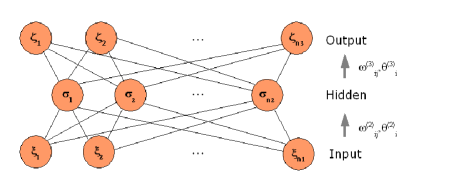
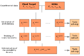
Figure 1: Left: a neural network. Right: Summary of the NNPDF approach.

3 Parton distributions

The strategy presented in the above section can be used to parametrize parton distributions, provided one now takes into account Altarelli-Parisi QCD evolution. Therefore we need to define a suitable evolution formalism, and we will consider for the sake of simplicity nonsinglet parton evolution. Since complex neural networks are not allowed, we must use the convolution theorem to evolve parton distributions in $x-$space using the inverse $\Gamma(x)$ of the Mellin space evolution factor $\Gamma(N)$, defined as

$$q(N,Q^{2})=q(N,Q_{0}^{2})\Gamma\left(N,\alpha_{s}\left(Q^{2}\right),\alpha_{s}\left(Q_{0}^{2}\right)\right)\ ,$$ (5)

$$\Gamma\left(x,\alpha_{s}\left(Q^{2}\right),\alpha_{s}\left(Q_{0}^{2}\right)\right)\equiv\frac{1}{2\pi i}\int_{c-i\infty}^{c+i\infty}dN~{}x^{-N}\Gamma\left(N,\alpha_{s}\left(Q^{2}\right),\alpha_{s}\left(Q_{0}^{2}\right)\right)\ .$$ (6)

The only subtlety is that eq. (6) defines a distribution, which must therefore be regulated at $x=1$, yielding the final evolution equation,

$$q(x,Q^{2})=q(x,Q_{0}^{2})\int_{x}^{1}dy~{}\Gamma(y)+\int_{x}^{1}\frac{dy}{y}\Gamma(y)\left(q\left(\frac{x}{y},Q_{0}^{2}\right)-yq(x,Q_{0}^{2})\right)\ ,$$ (7)

where in the above equation $q(x,Q_{0}^{2})$ is parametrized using a neural network. At higher orders in perturbation theory coefficient functions $C(N)$ are introduced through a modified evolution factor, $\tilde{\Gamma}(N)\equiv\Gamma(N)C(N)$. We have benchmarked our evolution code with the Les Houches benchmark tables Giele et al. (2002). The evolution factor $\Gamma(x)$ and its integral are computed and interpolated before the neural network training in order to have a faster fitting procedure.

As a first application of our method, we extract the nonsinglet parton distribution $q_{NS}(x,Q^{2}_{0})=\left(u+\bar{u}-d-\bar{d}\right)(x,Q^{2}_{0})$ from the nonsinglet structure function $F_{2}^{NS}(x,Q^{2})$ measured by the NMC Arneodo et al. (1997) and BCDMS Benvenuti et al. (1989, 1990) collaborations. The preliminary results of a NLO fit with fully correlated uncertainties can be seen in fig. 2. Our result is consistent within the error bands with the results from other global fits Martin et al. (2003); Stump et al. (2003); Alekhin (2003) in almost all the range of Bjorken-$x$. It is clear that the large uncertainties at small $x$ do not allow, within the current experimental data, to determine if $q_{NS}(x,Q^{2})$ grows at small $x$, as supported by different theoretical arguments as well as by other global parton fits. Only additional nonsinglet structure function data at small $x$ can settle this issue.

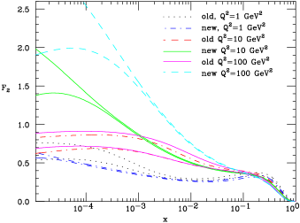
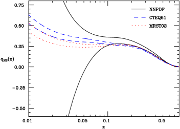
Figure 2: Left: The proton structure function, both the old version Forte et al. (2002) without HERA data and the new version Del Debbio et al. (2004) which included HERA data. Right: Preliminary results on the nonsinglet parton distribution $q_{NS}(x,Q_{0}^{2})$ compared with other global fits, for $Q_{0}^{2}=2~{}\mathrm{GeV}^{2}$

Summarizing, we have described a general technique to parametrize experimental data in an bias-free way with a faithful estimation of their uncertainties, which has been successfully applied to structure functions and that now is being implemented in the context of global parton distribution fits.

References

- Tung (2005) W.-K. Tung, AIP Conf. Proc., 753, 15–29 (2005), hep-ph/0410139.
- Forte et al. (2002) S. Forte, L. Garrido, J. I. Latorre, and A. Piccione, JHEP, 05, 062 (2002), hep-ph/0204232.
- Del Debbio et al. (2004) L. Del Debbio, S. Forte, J. I. Latorre, A. Piccione, and J. Rojo (2004), hep-ph/0501067.
- Stimpfl-Abele and Garrido (1991) G. Stimpfl-Abele, and L. Garrido, Comput. Phys. Commun., 64, 46–56 (1991).
- Rojo and Latorre (2004) J. Rojo, and J. I. Latorre, JHEP, 01, 055 (2004), hep-ph/0401047.
- Giele et al. (2002) W. Giele, et al. (2002), hep-ph/0204316.
- Arneodo et al. (1997) M. Arneodo, et al., Nucl. Phys., B483, 3–43 (1997), hep-ph/9610231.
- Benvenuti et al. (1989) A. C. Benvenuti, et al., Phys. Lett., B223, 485 (1989).
- Benvenuti et al. (1990) A. C. Benvenuti, et al., Phys. Lett., B237, 592 (1990).
- Martin et al. (2003) A. D. Martin, R. G. Roberts, W. J. Stirling, and R. S. Thorne, Eur. Phys. J., C28, 455–473 (2003), hep-ph/0211080.
- Stump et al. (2003) D. Stump, et al., JHEP, 10, 046 (2003), hep-ph/0303013.
- Alekhin (2003) S. Alekhin, Phys. Rev., D68, 014002 (2003), hep-ph/0211096.