Including the $\Delta(1232)$ resonance in baryon chiral perturbation theory

Abstract

Baryon chiral perturbation theory with explicit $\Delta(1232)$ degrees of freedom is considered. Using the extended on-mass-shell renormalization scheme, a manifestly Lorentz-invariant effective field theory with a systematic power counting is obtained. As applications we discuss the mass of the nucleon, the pion-nucleon sigma term, and the pole of the $\Delta$ propagator.

I Introduction

Chiral perturbation theory (ChPT) has been very successful in describing the vacuum sector of QCD at low energies Weinberg:1979kz ; Gasser:1984yg ; Gasser:1984gg . The sector with one baryon is more complicated. There, problems of obtaining a systematic power counting were encountered in the manifestly Lorentz-invariant formulation of the corresponding effective field theory (EFT) Gasser:1988rb . These problems have been handled in the framework of the so-called heavy-baryon chiral perturbation theory (HBChPT) Jenkins:1991jv ; Bernard:1992qa . Later the systematic power counting has also been restored in the original manifestly Lorentz-invariant formulation Tang:1996ca ; Ellis:1998kc ; Becher:1999he ; Gegelia:1999gf ; Gegelia:1999qt ; Fuchs:2003qc .

The strong coupling of the $\Delta(1232)$ resonance to the $\pi N$ channel and the relatively small mass difference between the nucleon and the delta motivate the inclusion of the $\Delta$ as an explicit dynamical degree of freedom in baryon chiral perturbation theory (BChPT). This has been done in a systematic way in the heavy-baryon formulation using the so-called “small scale expansion” (see, e.g., Ref. Hemmert:1997ye for an overview). A different power counting for the EFT with an explicit $\Delta$ degree of freedom has been considered in Refs. Pascalutsa:2002pi ; Pascalutsa:2004je .

When explicitly including the $\Delta$ resonance in BChPT, one has to deal with the whole complexity of a consistent interaction of higher-spin fields (see, e.g., Refs. Dirac:1936tg ; Fierz:1939ix ; Johnson:1960vt ; Velo:1969bt ). The problem is that, in a Lorentz-invariant formulation of a field theory involving particles of higher spin ($s\geq 1$), one necessarily introduces unphysical degrees of freedom. Physical degrees of freedom are defined on a surface specified by constraints. It turns out that it is rather non-trivial to write down interaction terms which respect the constraint structure of the theory. Various suggestions for constructing consistent interactions involving spin-3/2 particles can be found in, e.g., Refs. Nath:1971wp ; Tang:1996sq ; Pascalutsa:1998pw ; Pascalutsa:1999zz ; Deser:2000dz ; Pascalutsa:2000kd ; Pilling:2004wk ; Pilling:2004cu .

In this context we note that, as the low-energy EFT deals with small fluctuations of field variables around the vacuum, the problems showing up for stronger fields are not relevant to this theory. For such configurations the higher-order terms (infinite in number) generate contributions to physical quantities which are no longer suppressed by powers of small expansion parameters. Therefore, for large fluctuations the conclusions drawn from an analysis of a finite number of terms of the effective Lagrangian cannot be trusted. On the other hand, for small fluctuations around the vacuum one requires that the theory describes the right number of degrees of freedom in a self-consistent way. The interaction terms can be analyzed order by order in a small parameter expansion. Such an analysis leads to non-trivial constraints on the possible interactions.

In the present paper we consider the manifestly Lorentz-invariant form of BChPT with explicit $\Delta$ degrees of freedom. When using the standard formulation in combination with dimensional regularization one may face difficulties with respect to constructing the correct Lagrangian for spin-3/2 particles in $n$ space-time dimensions. Therefore, we apply the higher-derivative formulation of Ref. Djukanovic:2004px which is explicitly defined in four space-time dimensions. In order to generate a systematic power counting in the relevant EFT, we need to choose a suitable renormalization condition Becher:1999he ; Gegelia:1999gf ; Gegelia:1999qt ; Fuchs:2003qc . While the infrared regularization of Ref. Becher:1999he has been reformulated in a form which is also applicable to the effective theory with explicit resonance degrees of freedom Schindler:2003xv , we use the extended on-mass-shell (EOMS) renormalization scheme of Ref. Fuchs:2003qc in this work. Using as examples the one-loop contributions to the nucleon and $\Delta$ self-energies we demonstrate that there is a systematic power counting in the manifestly Lorentz-invariant formulation of the considered EFT. Other approaches, such as the twisted mass ChPT and chiral extrapolations in the framework of the covariant small scale expansion have recently been discussed in Refs. Walker-Loud:2005bt and Bernard:2005fy , respectively.

II The effective Lagrangian

In this section we will briefly discuss those elements of the most general effective Lagrangian which are relevant for the subsequent calculation of the nucleon mass and the pole of the $\Delta$ propagator at order $p^{3}$. All parameters and fields correspond to renormalized quantities. Counterterms are not explicitly shown.

II.1 Non-resonant Lagrangian

The non-resonant part of the effective Lagrangian consists of the sum of the purely mesonic and the $\pi N$ Lagrangians, respectively,

$${\cal L}_{\rm eff}={\cal L}_{\pi}+{\cal L}_{\pi N},$$

both of which are organized in a (chiral) derivative and quark-mass expansion (see, e.g., Ref. Scherer:2002tk for an introduction),

$${\cal L}_{\pi} = {\cal L}_{2}+{\cal L}_{4}+\cdots,$$

$${\cal L}_{\pi N} = {\cal L}_{\pi N}^{(1)}+{\cal L}_{\pi N}^{(2)}+{\cal L}_{\pi N}^{(3)}+\cdots,$$

where the subscripts (superscripts) in ${\cal L}_{\pi}$ (${\cal L}_{\pi N}$) refer to the order in the expansion. The lowest-order mesonic Lagrangian reads Gasser:1984yg

$${\cal L}_{2}=\frac{F^{2}}{4}\mbox{Tr}\left[D_{\mu}U\left(D^{\mu}U\right)^{\dagger}\right]+\frac{F^{2}}{4}\mbox{Tr}\left(\chi U^{\dagger}+U\chi^{\dagger}\right).$$ (1)

The pion fields are contained in the unimodular unitary $(2\times 2)$ matrix $U$ which, under a local $\mbox{SU}(2)_{L}\times\mbox{SU}(2)_{R}\times\mbox{U}(1)_{V}$ transformation denoted by the group element $(V_{L}(x),V_{R}(x),\exp[-i\Theta(x)])$, transforms as

$$U\mapsto U^{\prime}=V_{R}UV_{L}^{\dagger}.$$ (2)

Introducing external fields $l_{\mu}$ and $r_{\mu}$ transforming as

$$l_{\mu} \mapsto V_{L}l_{\mu}V_{L}^{\dagger}+iV_{L}\partial_{\mu}V_{L}^{\dagger},$$

$$r_{\mu} \mapsto V_{R}r_{\mu}V_{R}^{\dagger}+iV_{R}\partial_{\mu}V_{R}^{\dagger},$$

the covariant derivative is defined as

$$D_{\mu}U=\partial_{\mu}U-ir_{\mu}U+iUl_{\mu}.$$

In Eq. (1), $F$ denotes the pion-decay constant in the chiral limit: $F_{\pi}=F[1+{\cal O}(\hat{m})]=92.4$ MeV. Moreover,

$$\chi=2B(s+ip)$$

contains external scalar and pseudoscalar fields transforming as $\chi\mapsto V_{R}\,\chi\,V_{L}^{\dagger}$. We work in the isospin-symmetric limit $m_{u}=m_{d}=\hat{m}$ and the lowest-order expression for the squared pion mass is $M^{2}=2B\hat{m}$, where $B$ is related to the scalar quark condensate in the chiral limit Gasser:1984yg , $\langle 0|\bar{u}u|0\rangle=\langle 0|\bar{d}d|0\rangle=-F^{2}B$.

To improve the ultraviolet behavior of the pion propagator and to regulate the loop diagrams calculated in this work, we use the higher-derivative formulation of Ref. Djukanovic:2004px . We include the following additional terms in the effective Lagrangian:

$${\cal L}_{\pi\pi}^{\rm reg}=\sum\limits_{n=1}^{N_{\pi}}\frac{X_{n}}{4}\ \frac{F^{2}}{4}\ {\rm Tr}\left(\left\{\left(D^{2}\right)^{n}UU^{\dagger}-U\left[\left(D^{2}\right)^{n}U\right]^{\dagger}\right\}\left[D^{2}UU^{\dagger}-U\left(D^{2}U\right)^{\dagger}-\chi U^{\dagger}+U\chi^{\dagger}\right]\right),$$

where $D^{2}U=D_{\alpha}D^{\alpha}U$ and $X_{n}$ are free parameters. For our calculations we take $N_{\pi}=4$ and choose the parameters $X_{i}$ as

$$X_{1} = \frac{4}{\Lambda^{2}},$$

$$X_{2} = \frac{6}{\Lambda^{4}},$$

$$X_{3} = \frac{4}{\Lambda^{6}},$$

$$X_{4} = \frac{1}{\Lambda^{8}},$$ (3)

resulting in the modified pion Feynman propagator

$$\Delta^{\Lambda}_{\pi}(p)=\frac{1}{p^{2}-M^{2}+i0^{+}}\,\frac{\left(-\Lambda^{2}\right)^{4}}{\left(p^{2}-\Lambda^{2}+i0^{+}\right)^{4}}.$$ (4)

Here, $\Lambda$ is a free parameter which plays the role of a regulator in the loop diagrams.

Let $\Psi=(p,n)^{T}$ denote the nucleon field with two four-component Dirac fields $p$ and $n$ describing the proton and neutron, respectively, transforming as

$$\Psi\mapsto\Psi^{\prime}=\exp[-i\Theta]K[V_{L},V_{R},U]\Psi,$$ (5)

where

$$K[V_{L},V_{R},U]=\sqrt{V_{R}UV_{L}^{\dagger}}^{-1}V_{R}\sqrt{U}.$$ (6)

The $\pi N$ Lagrangian is bilinear in $\bar{\Psi}$ and $\Psi$ and involves the quantities $u$, $u_{\mu}$, $\Gamma_{\mu}$, and $\chi_{\pm}$ (and their derivatives):

$$u^{2} = U,$$

$$u_{\mu} = i\left[u^{\dagger}\left(\partial_{\mu}-ir_{\mu}\right)u-u\left(\partial_{\mu}-il_{\mu}\right)u^{\dagger}\right],$$

$$\Gamma_{\mu} = \frac{1}{2}\,\left[u^{\dagger}\left(\partial_{\mu}-ir_{\mu}\right)u+u\left(\partial_{\mu}-il_{\mu}\right)u^{\dagger}\right],$$

$$\chi_{\pm} = u^{\dagger}\chi u^{\dagger}\pm u\chi^{\dagger}u.$$

In terms of these building blocks the lowest-order Lagrangian reads Gasser:1988rb

$${\cal L}_{\pi N}^{(1)}=\bar{\Psi}\left(i\gamma_{\mu}D^{\mu}-m+\frac{1}{2}\stackrel{{\scriptstyle\circ}}{{g}}_{A}\gamma_{\mu}\gamma_{5}u^{\mu}\right)\Psi,$$ (7)

where the covariant derivative is defined as

$$D_{\mu}\Psi=(\partial_{\mu}+\Gamma_{\mu}-iv_{\mu}^{(s)})\Psi$$

with the external field transforming as $v_{\mu}^{(s)}\mapsto v_{\mu}^{(s)}-\partial_{\mu}\Theta$. Finally, $m$ denotes the mass of the nucleon at leading order in the expansion in small parameters and $\stackrel{{\scriptstyle\circ}}{{g}}_{\!A}$ refers to the chiral limit of the axial-vector coupling constant.

For our purposes, we only need to consider one of the seven structures of the Lagrangian at ${\cal O}(p^{2})$ Gasser:1988rb

$${\cal L}_{\pi N}^{(2)}=\tilde{c}_{1}\mbox{Tr}(\chi_{+})\bar{\Psi}\Psi+\cdots,$$ (8)

where $\tilde{c}_{1}$ refers to the coupling constant in the theory explicitly including delta degrees of freedom. The Lagrangian ${\cal L}^{(3)}_{\pi N}$ does not contribute in our calculations.

II.2 Lagrangian of the $\Delta(1232)$ resonance

In order to write down the Lagrangian of the $\Delta(1232)$ resonance [$I(J^{P})=\frac{3}{2}(\frac{3}{2}^{+})$] we introduce the vector-spinor isovector-isospinor fields

$$\Psi_{\mu,i}=\left(\begin{array}[]{c}\Psi_{\mu,i,\frac{1}{2}}\\ \Psi_{\mu,i,-\frac{1}{2}}\end{array}\right),\quad\mu=0,1,2,3,\quad i=1,2,3,$$ (9)

i.e., for any values of $\mu$ and $i$ the component $\Psi_{\mu,i}$ consists of an isospin doublet of Dirac spinors. The delta field components transform as Tang:1996sq

$$\Psi_{\mu,i,\alpha}\mapsto\Psi_{\mu,i,\alpha}^{\prime}=\exp[-i\Theta]{\cal K}_{ij,\alpha\beta}\Psi_{\mu,j,\beta},$$ (10)

where

$${\cal K}_{ij,\alpha\beta}=\frac{1}{2}\mbox{Tr}(\tau_{i}K\tau_{j}K^{\dagger})K_{\alpha\beta}$$ (11)

with $K$ defined in Eq. (6). The corresponding covariant derivative is given by

$$(D_{\mu}\Psi)_{\nu,i,\alpha} \equiv {\cal D}_{\mu,ij,\alpha\beta}\Psi_{\nu,j,\beta},$$

$${\cal D}_{\mu,ij,\alpha\beta} = \partial_{\mu}\delta_{ij}\delta_{\alpha\beta}-2i\epsilon_{ijk}\Gamma_{\mu,k}\delta_{\alpha\beta}+\delta_{ij}\Gamma_{\mu,\alpha\beta}-iv_{\mu}^{(s)}\delta_{ij}\delta_{\alpha\beta},$$

where we parameterized $\Gamma_{\mu}=\tau_{k}\Gamma_{\mu,k}$. The description of Eq. (9) involves 6 (uncoupled) isospin components whereas the physical delta consists of an isospin quadruplet. Introducing the isospin projection operators

$$\xi^{\frac{3}{2}}_{ij,\alpha\beta} = \delta_{ij}\delta_{\alpha\beta}-\frac{1}{3}(\tau_{i}\tau_{j})_{\alpha\beta},$$ (12)

$$\xi^{\frac{1}{2}}_{ij,\alpha\beta} = \frac{1}{3}(\tau_{i}\tau_{j})_{\alpha\beta},$$ (13)

the leading-order Lagrangian is given by Hemmert:1997ye

$${\cal L}_{\Delta}^{(1)}=\bar{\Psi}_{\mu}\xi^{\frac{3}{2}}\Lambda^{\mu\nu}\xi^{\frac{3}{2}}\Psi_{\nu},$$ (14)

where

$$\Lambda_{\mu\nu} = -\Biggl{[}(i{D/\hskip 1.00006pt}-m_{\Delta})\,g_{\mu\nu}+iA\,(\gamma_{\mu}D_{\nu}+\gamma_{\nu}D_{\mu})$$ (15)

$$+\frac{i}{2}\,(3A^{2}+2A+1)\,\gamma_{\mu}{D/\hskip 1.00006pt}\gamma_{\nu}+m_{\Delta}\,(3A^{2}+3A+1)\,\gamma_{\mu}\gamma_{\nu}$$

$$+\frac{g_{1}}{2}\,u/\,\gamma_{5}\,g_{\mu\nu}+\frac{g_{2}}{2}\,\left(\gamma_{\mu}u_{\nu}+u_{\mu}\gamma_{\nu}\right)\gamma_{5}+\frac{g_{3}}{2}\,\gamma_{\mu}u/\,\gamma_{5}\gamma_{\nu}\Biggr{]}.$$

Here, $A$ is an arbitrary real parameter except that $A\neq-1/2$ and $m_{\Delta}$ denotes the mass of the $\Delta$ at leading order in the expansion in small parameters.

The Lagrangian of Eq. (14) describes a system with constraints. Using the canonical formalism (i.e. canonical coordinates and momenta and the corresponding Hamiltonian) we have analyzed the structure of the constraints in analogy with Refs. Nath:1971wp ; Pascalutsa:1998pw . Demanding that the above interaction terms lead to a consistent theory with the correct number of physical degrees of freedom we obtain after a lengthy calculation the following relations among the coupling constants Wies:2005 :

$$g_{2}=A\,g_{1}\,,\quad g_{3}=-\frac{1+2\,A+3\,A^{2}}{2}\ g_{1}.$$ (16)

In other words, what seem to be independent interaction terms from the point of view of constructing the most general Lagrangian Hemmert:1997ye , turn out to be related once the self consistency conditions are imposed. This situation is similar to the case of the universal $\rho$-meson coupling recently discussed in Ref. Djukanovic:2004mm . There, relations among coupling constants were obtained from the requirement of the consistency of EFT with respect to renormalization.

The Lagrangian of Eq. (14) with the couplings of Eq. (16) is invariant under the set of transformations

$$\Psi_{\mu} \rightarrow \Psi_{\mu}+a\gamma_{\mu}\gamma^{\nu}\Psi_{\nu}\,,$$ (17)

$$A \rightarrow \frac{A-2\,a}{1+4\,a}$$ (18)

which are often referred to as a point transformation Nath:1971wp ; Tang:1996sq . The change of field variables of Eq. (17) generates a (new) Lagrangian ${\cal L}(\Psi_{\mu},g_{1},A+2a+4aA)$ which, as a consequence of the equivalence theorem Kamefuchi:1961sb , must yield the same observables as the original Lagrangian ${\cal L}(\Psi_{\mu},g_{1},A)$. Since $a$ can be chosen arbitrarily except that $a\neq-1/4$, physical quantities cannot depend on $A$ Nath:1971wp ; Tang:1996sq . We will use $A=-1$ in our calculations. It is worth emphasizing that we did not require the invariance under the point transformation to begin with; rather it comes out automatically as a consequence of consistency in the sense of having the right number of degrees of freedom. Moreover, demanding the invariance under the point transformation alone would not be sufficient to obtain the relations of Eq. (16). For example, in Ref. Tang:1996sq three $\pi\Delta\Delta$ interactions involving one overall coupling constant and two additional “off-shell parameters” were introduced so as to preserve the invariance under the point transformation. It was then shown that the contributions to physical quantities, generated by the two interaction terms corresponding to the above coupling constants $g_{2}$ and $g_{3}$, can be systematically included in redefinitions of coupling constants of an infinite number of local terms in the Lagrangian. As we are unable to analyze all of these structures and decide if they are allowed by consistency conditions (in the sense of generating the correct number of degrees of freedom), we choose to use the above values of Eq. (16), which are certainly consistent.

The effective Lagrangian of Eq. (14) is also invariant under the following local transformations

$$\Psi_{\mu,i}(x)\to\Psi_{\mu,i}(x)+\tau_{i}\alpha_{\mu}(x),$$ (19)

where $\alpha_{\mu}$ is an arbitrary vector-spinor isospinor function. This is due to the fact that we use six isospin degrees of freedom $\Psi_{\mu,i,\alpha}(x)$ instead of four physical isospin degrees of freedom. We could make use of Eq. (70) and rewrite the Lagrangian in terms of the physical fields, but for reasons of convenience we prefer to work with the gauge-invariant Lagrangian.

The quantization of the effective Lagrangian of Eq. (14) with the gauge fixing condition $\tau_{i}\Psi_{\mu,i}=0$ leads to the following Feynman propagator

$$S^{\mu\nu}_{0,ij,\alpha\beta}(p)=\xi^{\frac{3}{2}}_{ij,\alpha\beta}S^{\mu\nu}_{0}(p),$$ (20)

where

$$S^{\mu\nu}_{0}(p) = -\frac{p/\hskip 1.00006pt+m_{\Delta}}{p^{2}-m_{\Delta}^{2}+i0^{+}}\,\Biggl{[}g^{\mu\nu}-\frac{1}{3}\,\gamma^{\mu}\gamma^{\nu}+\frac{1}{3m_{\Delta}}\left(p^{\mu}\gamma^{\nu}-\gamma^{\mu}p^{\nu}\right)-\frac{2}{3m_{\Delta}^{2}}\,p^{\mu}p^{\nu}\Biggr{]}$$

$$+\frac{1}{3m_{\Delta}^{2}}\,\frac{1+A}{1+2A}\,\Biggl{\{}\left[\frac{A}{1+2A}\,m_{\Delta}-\frac{1+A}{2(1+2A)}p/\hskip 1.00006pt\right]\gamma^{\mu}\gamma^{\nu}-\gamma^{\mu}p^{\nu}-\frac{A}{1+2A}\,p^{\mu}\gamma^{\nu}\Biggr{\}}.$$

In particular, choosing $A=-1$ results in the most convenient expression for the free delta Feynman propagator.

From the Lagrangian at ${\cal O}(p^{2})$ we only need one term, namely,

$${\cal L}_{\Delta}^{(2)}=-c_{1}^{\Delta}\mbox{Tr}(\chi_{+})\bar{\Psi}_{\mu,i}\,\xi_{ij}^{\frac{3}{2}}\,g^{\mu\nu}\,\Psi_{\nu,j}.$$ (21)

II.3 $\pi N\Delta$ interaction term

The leading-order $\pi N\Delta$ interaction Lagrangian can be written as

$${\cal L}_{\pi N\Delta}^{(1)}=-g\,\bar{\Psi}_{\mu,i}\,\xi^{\frac{3}{2}}_{ij}\,(g^{\mu\nu}+\tilde{z}\,\gamma^{\mu}\gamma^{\nu})\,u_{\nu,j}\,\Psi+h.c.\,,$$ (22)

where we parameterized $u_{\mu}=\tau_{k}u_{\mu,k}$ , and $g$ and $\tilde{z}$ are coupling constants. The analysis of the structure of constraints yields

$$\tilde{z}=\frac{3\,A+1}{2}.$$ (23)

Again, the interaction term of Eq. (22) with the coupling constants $g$ and $\tilde{z}$ constrained by Eq. (23) is invariant under the point transformation of Eqs. (17) and (18).

II.4 Power counting

We organize our perturbative calculations by applying the standard power counting of Refs. Weinberg:1991um ; Ecker:1995gg to the renormalized diagrams, i.e., an interaction vertex obtained from an ${\cal O}(p^{n})$ Lagrangian counts as order $p^{n}$, a pion propagator as order $p^{-2}$, a nucleon propagator as order $p^{-1}$, and the integration of a loop as order $p^{4}$. In addition, we assign the order $p^{-1}$ to the $\Delta$ propagator and the order $p^{1}$ to the mass difference $\delta\equiv m_{\Delta}-m$. As will be demonstrated below, this power counting is respected by the renormalized loop diagrams within the EOMS renormalization scheme of Ref. Fuchs:2003qc .

III Nucleon mass

In this section we calculate the nucleon mass to order $p^{3}$. To that end we consider the two-point function of the nucleon

$$-i\int d^{4}xe^{ip\cdot x}\langle 0|T[\Psi(x)\bar{\Psi}(0)]|0\rangle=\frac{1}{p/\,-m-\Sigma(p/)},$$ (24)

where $\Sigma$ is the self-energy of the nucleon. The nucleon mass is identified in terms of the pole of Eq. (24) at $p/\,=m_{N}$.

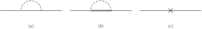
Figure 1: One-loop contributions to the nucleon self-energy at ${\cal O}(p^{3})$.

Equation (8) generates the constant tree-level contribution $-4\,\tilde{c}_{1}M^{2}$ to the self-energy at ${\cal O}(p^{2})$. The unrenormalized one-loop contribution resulting from Fig. 1 (a) has the form

$$\Sigma_{N}^{\rm loop}=-\frac{3\stackrel{{\scriptstyle\circ}}{{g}}_{\!A}^{2}\Lambda^{8}}{4F^{2}}\left[\gamma_{\mu}\left(-p/\hskip 1.00006pt+m\right)\gamma_{\nu}\ I^{\mu\nu}_{m}(411)-g_{\mu\nu}\gamma_{\lambda}\ I^{\mu\nu\lambda}_{m}(411)\right],$$ (25)

where

$$\left\{I_{m}(abc),I^{\mu\nu}_{m}(abc),I^{\mu\nu\lambda}_{m}(abc)\right\}=i\int\frac{d^{4}k}{(2\pi)^{4}}\frac{\left\{1,k^{\mu}k^{\nu},k^{\mu}k^{\nu}k^{\lambda}\right\}}{A^{a}B^{b}C^{c}_{m}},$$ (26)

with

$$A=k^{2}-\Lambda^{2}+i0^{+},$$

$$B=k^{2}-M^{2}+i0^{+},$$

$$C_{m}=(p+k)^{2}-m^{2}+i0^{+}.$$

Substituting the results of the loop integrals of Appendix C into Eq. (25), we obtain

$$\Sigma_{N}^{\rm loop}(p/\,=m_{N}) = -\frac{\stackrel{{\scriptstyle\circ}}{{g}}_{\!A}^{2}\,m}{32\,\pi^{2}\,F^{2}}\,\left[\Lambda^{2}+7\,m^{2}-6\,m^{2}\ln\left(\frac{\Lambda}{m}\right)\right]$$ (27)

$$-\frac{\stackrel{{\scriptstyle\circ}}{{g}}_{\!A}^{2}M^{2}}{64\,\pi^{2}\,F^{2}}\,\left[5\,m-24\,\tilde{c}_{1}\,m^{2}-4\,\tilde{c}_{1}\,\Lambda^{2}-12\,m\,\ln\left(\frac{\Lambda}{m}\right)\right]$$

$$-\frac{3\,\stackrel{{\scriptstyle\circ}}{{g}}_{\!A}^{2}M^{3}}{32\,\pi\,F^{2}}.$$

Within the EOMS renormalization scheme Fuchs:2003qc the first two lines of Eq. (27) are canceled by the corresponding contributions of the counterterm diagram of Fig. 1 (c), leaving the last line of Eq. (27) as the ${\cal O}(p^{3})$ contribution of the renormalized diagram of Fig. 1 (a). The unrenormalized one-loop contribution of the $\Delta$ resonance of Fig. 1 (b) reads thanks

$$\Sigma_{\Delta}^{\rm loop}=\,\frac{4\,g^{2}\,\Lambda^{8}}{3\,m_{\Delta}^{2}F^{2}}\left[\left(p/\hskip 1.00006pt+m_{\Delta}\right)\left(p_{\mu}p_{\nu}-p^{2}g_{\mu\nu}\right)I^{\mu\nu}_{m_{\Delta}}(411)+\gamma_{\lambda}\left(p_{\mu}p_{\nu}-p^{2}g_{\mu\nu}\right)I^{\mu\nu\lambda}_{m_{\Delta}}(411)\right].$$ (28)

The corresponding contribution to the mass of the nucleon is obtained from

$$\Sigma_{\Delta}^{\rm loop}(p/\,=m_{N}) = \frac{5\,g^{2}}{1152\,\pi^{2}\,F^{2}}\left[-8\,m\,\,\Lambda^{2}-21\,m^{3}+24\,m^{3}\,\ln\left(\frac{\Lambda}{m}\right)\right]$$ (29)

$$+\frac{g^{2}\,\delta}{576\,\pi^{2}\,F^{2}}\left[28\,\Lambda^{2}-135\,m^{2}+120\,m^{2}\,\ln\left(\frac{\Lambda}{m}\right)\right]$$

$$+\frac{g^{2}}{384\,\pi^{2}\,F^{2}\,m}\left[4\,\tilde{c}_{1}\,M^{2}\,m\,\left(32\,\Lambda^{2}+55\,m^{2}\right)-3\,\delta^{2}\,\left(8\,\Lambda^{2}+35\,m^{2}\right)\right]$$

$$-\frac{5\,m\,g^{2}}{48\,\pi^{2}\,F^{2}}\left[\delta^{2}+2\,M^{2}\,\left(2\,\tilde{c}_{1}\,m-1\right)\right]\,\ln\left(\frac{\Lambda}{m}\right)$$

$$+\frac{g^{2}\,\Lambda^{2}}{144\,\pi^{2}\,F^{2}\,m^{2}}\left(11\,\delta^{3}-72\,\tilde{c}_{1}\,\delta\,M^{2}\,m\right)$$

$$+\frac{g^{2}}{24\,\pi^{2}\,F^{2}}\,\left[3\,\delta^{3}-M^{2}\,\delta\left(7+60\,\tilde{c}_{1}\,m\right)\right]\,\ln\left(\frac{\Lambda}{m}\right)$$

$$+\frac{g^{2}}{288\,\pi^{2}\,F^{2}}\Biggl{[}35\,\delta^{3}+6\,\delta\,M^{2}\left(1+25\,\tilde{c}_{1}\,m\right)$$

$$+96\,\left(\delta^{2}-M^{2}\right)^{3/2}\,\ln\left(\frac{\delta-\sqrt{\delta^{2}-M^{2}}}{M}\right)\Bigg{]}$$

$$-\frac{g^{2}}{6\,\pi^{2}\,F^{2}}\,\left(2\,\delta^{3}-3\,M^{2}\,\delta\right)\,\ln\left(\frac{M}{m}\right).$$

Again, in the EOMS renormalization scheme the first six lines of Eq. (29) are canceled by the corresponding contributions of the counterterm diagram of Fig. 1 (c), leaving the last three lines of Eq. (29) as the delta loop contribution to the nucleon mass at ${\cal O}(p^{3})$. Combining the tree-level result at ${\cal O}(p^{2})$ with the ${\cal O}(p^{3})$ one-loop contributions we obtain the following expression for the nucleon mass:

$$m_{N} = m-4\,\tilde{c}_{1}M^{2}-{3\,\stackrel{{\scriptstyle\circ}}{{g}}_{\!A}^{2}\,M^{3}\over 32\,\pi\,F^{2}}+\frac{g^{2}}{288\,\pi^{2}\,F^{2}}\Biggl{[}35\,\delta^{3}+6\,\delta\,M^{2}\,\left(1+25\,\tilde{c}_{1}\,m\right)$$ (30)

$$+96\,\left(\delta^{2}-M^{2}\right)^{3/2}\,\ln\left(\frac{\delta-\sqrt{\delta^{2}-M^{2}}}{M}\right)\Bigg{]}$$

$$-\frac{g^{2}}{6\,\pi^{2}\,F^{2}}\,\left(2\,\delta^{3}-3\,M^{2}\,\delta\right)\,\ln\left(\frac{M}{m}\right)+{\cal O}\left(p^{4}\right),$$

which is in agreement with Ref. Bernard:2003xf .

By explicitly including the spin-3/2 degrees of freedom, terms of higher order in the chiral expansion have been re-summed. In order to obtain the numerical value of these terms, we expand Eq. (30) in powers of $M$ and match the terms of orders $M^{0}$ and $M^{2}$, respectively, to the corresponding quantities of the EFT without explicit spin-3/2 degrees of freedom. Taking into account that there are no tree-level $\Delta$ contributions to $c_{1}$ Becher:1999he , we obtain

$$\,\stackrel{{\scriptstyle\circ}}{{m}}\,=m+\frac{g^{2}\,\delta^{3}}{3\,\pi^{2}\,F^{2}}\ln\left(\frac{m}{2\delta}\right)+\frac{35\,g^{2}\,\delta^{3}}{288\,\pi^{2}\,F^{2}}\,,$$ (31)

$$c_{1}=\tilde{c}_{1}-(1+5\,\tilde{c}_{1}\,m)\frac{5\,g^{2}\,\delta}{192\,\pi^{2}\,F^{2}}+\frac{g^{2}\,\delta}{8\,\pi^{2}\,F^{2}}\,\ln\left(\frac{m}{2\delta}\right),$$ (32)

where $\,\stackrel{{\scriptstyle\circ}}{{m}}\,$ denotes the nucleon mass in the chiral limit and $c_{1}$ replaces the coupling constant of Eq. (8) in the theory without spin-3/2 degrees of freedom. Using Eqs. (31) and (32), the nucleon mass of Eq. (30) can be rewritten as

$$m_{N} = \,\stackrel{{\scriptstyle\circ}}{{m}}\,-4\,c_{1}M^{2}-{3\,\stackrel{{\scriptstyle\circ}}{{g}}_{\!A}^{2}\,M^{3}\over 32\,\pi\,F^{2}}+\tilde{m}_{N},$$ (33)

where $\tilde{m}_{N}\sim M^{4}$ and contains an infinite number of terms if expanded in powers of $M/\delta$.

In order to calculate the numerical value of $\tilde{m}_{N}$, we make use of $g=1.127$ as obtained from a fit to the $\Delta\to\pi N$ decay width, and take the numerical values

$$g_{A}=1.267,\quad F_{\pi}=92.4\,\mbox{MeV},\quad m_{N}=m_{p}=938.3\,\mbox{MeV},$$

$$M_{\pi}=M_{\pi^{+}}=139.6\,\mbox{MeV},\quad m_{\Delta}=1210\,\mbox{MeV},\,\delta=m_{\Delta}-m_{N}.$$ (34)

Substituting the above values in the expression for $\tilde{m}_{N}$ results in

$$\tilde{m}_{N}=-5.7\,\mbox{MeV}.$$ (35)

We recall that an analysis of the nucleon mass up to and including order $M^{4}$ Fuchs:2003kq yields $(882.8+74.8-15.3)\,\mbox{MeV}=942.3$ MeV for the first three terms of Eq. (33). This analysis made use of $c_{1}=-0.9\,m_{N}^{-1}$ Becher:2001hv as obtained from a (tree-level) fit to the $\pi N$ scattering threshold parameters of Ref. Koch:bn and a value of 45 MeV Gasser:1990ce for the pion-nucleon sigma term to be discussed below. In other words, the explicit inclusion of the spin-3/2 degrees of freedom does not have a significant impact on the nucleon mass.

Applying the Hellmann-Feynman theorem Hellmann ; Feynman to the nucleon mass Gasser:1984yg ; Gasser:1988rb ; Lehnhart:2004vi

$$\sigma=M^{2}\frac{\partial m_{N}}{\partial M^{2}},$$ (36)

the pion-nucleon sigma term to order $p^{3}$ reads

$$\sigma = -4\,\tilde{c}_{1}M^{2}-\frac{9\,\stackrel{{\scriptstyle\circ}}{{g}}_{\!A}^{2}M^{3}}{64\,\pi\,F^{2}}+\frac{5\,g^{2}\,(1+5\,\tilde{c}_{1}\,m)\,\delta\,M^{2}}{48\,\pi^{2}\,F^{2}}$$ (37)

$$-\frac{g^{2}\,(\delta^{2}-M^{2})^{\frac{1}{2}}\,M^{2}}{2\,\pi^{2}\,F^{2}}\,\ln\left(\frac{\delta-\sqrt{\delta^{2}-M^{2}}}{M}\right)+\frac{g^{2}\,\delta\,M^{2}}{2\,\pi^{2}\,F^{2}}\,\ln\left(\frac{M}{m}\right).$$

Again, expanding Eq. (37) in powers of $M$ and using Eq. (32), we rewrite $\sigma$ as

$$\sigma=-4\,c_{1}M^{2}-\frac{9\,\stackrel{{\scriptstyle\circ}}{{g}}_{\!A}^{2}M^{3}}{64\,\pi\,F^{2}}+\tilde{\sigma},$$ (38)

where $\tilde{\sigma}$ is of order $M^{4}$ and contains an infinite number of terms if expanded in powers of $M/\delta$. With the numerical values of Eq. (III) we obtain from Eq. (37)

$$\tilde{\sigma}=-10.2\,\mbox{MeV},$$ (39)

while the first two terms of Eq. (38) yield $(74.8-22.9)\,\mbox{MeV}=51.9$ MeV. These numbers have to be compared with the empirical values of the sigma term extracted from data on pion-nucleon scattering: 40 MeV Buettiker:1999ap , $(45\pm 5)$ MeV Gasser:1990ce , and $(64\pm 7)$ MeV Pavan:2001wz . Equation (39) indicates that the explicit inclusion of the spin-3/2 degrees of freedom plays a more important role for the sigma term than for the nucleon mass. However, one has to keep in mind that the sigma term only starts at order $M^{2}$ and thus, on a relative scale, is automatically more sensitive to higher-order corrections.

IV Pole of the $\Delta$ propagator

Using isospin symmetry, the isospin structure of the dressed $\Delta$ propagator is given by

$$S^{\mu\nu}_{ij,\alpha\beta}(p)=\xi^{\frac{3}{2}}_{ij,\alpha\beta}S^{\mu\nu}(p),$$ (40)

where $S^{\mu\nu}(p)$ is obtained by solving the equation

$$S^{\mu\nu}(p)=S_{0}^{\mu\nu}(p)-S^{\mu\rho}(p)\Sigma_{\rho\sigma}(p)S_{0}^{\sigma\nu}(p).$$ (41)

Here, $S_{0}^{\mu\nu}(p)$ refers to the free Feynman propagator of Eq. (20) and $i\,\Sigma^{\mu\nu}$ originates from the sum of the one-particle-irreducible diagrams contributing to the two-point function of the $\Delta$. The solution of Eq. (41) has a rather complicated form Kaloshin:2003xc , but at this stage we are only interested in determining the pole of the dressed propagator. For that purpose we may contract Eq. (41) with appropriate vector spinors,

$$\bar{u}_{\mu}S^{\mu\nu}u_{\nu}=\bar{u}_{\mu}S_{0}^{\mu\nu}u_{\nu}-\bar{u}_{\mu}S^{\mu\rho}\Sigma_{\rho\sigma}S_{0}^{\sigma\nu}u_{\nu},$$ (42)

where

$$\gamma^{\mu}\,u_{\mu} = 0,$$

$$p^{\mu}\,u_{\mu} = 0,$$ (43)

with corresponding expressions for the adjoints. We parameterize the dressed propagator and the self-energy of the $\Delta$ resonance as

$$\Sigma^{\mu\nu}=\sum_{a=1}^{10}\Sigma_{a}{\cal P}_{a}^{\mu\nu},$$ (44)

$$S^{\mu\nu}=\sum_{a=1}^{10}S_{a}{\cal P}_{a}^{\mu\nu},$$ (45)

where the $\Sigma_{a}$ and $S_{a}$ are functions of $p^{2}$, and the basis $\{{\cal P}_{a}^{\mu\nu}\}$ is specified in Appendix B. Using the identities

$$\bar{u}_{\mu}S^{\mu\nu} = \bar{u}^{\nu}\left(S_{1}+p/\hskip 1.00006ptS_{6}\right),$$ (46)

$$\bar{u}_{\mu}S_{0}^{\mu\nu} = -\frac{\bar{u}^{\nu}\left(p/\hskip 1.00006pt+m_{\Delta}\right)}{p^{2}-m_{\Delta}^{2}}\,,$$ (47)

$$S_{0}^{\mu\nu}u_{\nu} = -\frac{\left(p/\hskip 1.00006pt+m_{\Delta}\right)u^{\mu}}{p^{2}-m_{\Delta}^{2}},$$ (48)

we solve Eq. (42) for $S_{1}$ and $S_{6}$:

$$S_{1} = \frac{m_{\Delta}+\Sigma_{1}}{\left(m_{\Delta}+\Sigma_{1}\right)^{2}-p^{2}\left(1-\Sigma_{6}\right)^{2}},$$ (49)

$$S_{6} = \frac{1-\Sigma_{6}}{\left(m_{\Delta}+\Sigma_{1}\right)^{2}-p^{2}\left(1-\Sigma_{6}\right)^{2}}\,.$$ (50)

As was to be expected, both scalar functions $S_{1}$ and $S_{6}$ have the same poles.

The pole is found by solving the equation

$$x=f(x)$$ (51)

with

$$f(x)=\frac{[m_{\Delta}+\Sigma_{1}(x)]^{2}}{[1-\Sigma_{6}(x)]^{2}}.$$ (52)

Performing a loop expansion for both the function $f(x)$ as well as the solution $y$ to Eq. (51),

$$f(x) = \sum_{i=0}^{\infty}\hbar^{i}\,f^{(i)}(x),$$

$$y = \sum_{j=0}^{\infty}\hbar^{j}y^{(j)},$$

we obtain up to and including order $\hbar$:

$$y^{(0)}+\hbar y^{(1)}+O(\hbar^{2})=y^{(0)}+\hbar\frac{f^{(1)}(y^{(0)})}{1-f^{(0)^{\prime}}(y^{(0)})}+O(\hbar^{2}).$$

In fact, using suitable field redefinitions Kamefuchi:1961sb ; Scherer:1994wi , in a first step any dependence on $p^{2}$ of the tree-level contribution to the self-energy can be removed, i.e. $f^{(0)^{\prime}}(x)=0$. We then obtain, setting $\hbar=1$,

$$s=s^{(0)}+s^{(1)}+\cdots$$ (53)

for the pole $s$ of the $\Delta$ propagator to one-loop order, where

$$s^{(0)} = \frac{\left(m_{\Delta}+\Sigma_{1}^{(0)}\right)^{2}}{\left(1-\Sigma_{6}^{(0)}\right)^{2}},$$

$$s^{(1)} = 2\frac{m_{\Delta}+\Sigma_{1}^{(0)}}{\left(1-\Sigma_{6}^{(0)}\right)^{3}}\left[(m_{\Delta}+\Sigma_{1}^{(0)})\Sigma_{6}^{(1)}(p^{2})+(1-\Sigma_{6}^{(0)})\Sigma_{1}^{(1)}(p^{2})\right]_{p^{2}=s^{(0)}}.$$

In a second step, using again a suitable field redefinition, the tree-level contribution proportional to ${\cal P}_{6}^{\mu\nu}=g^{\mu\nu}p/\,$, i.e. $\Sigma_{6}^{(0)}$, can also be removed and the result simplifies even further,

$$s=\left(m_{\Delta}+\Sigma_{1}^{(0)}\right)^{2}+2\left(m_{\Delta}+\Sigma_{1}^{(0)}\right)\left[\left(m_{\Delta}+\Sigma_{1}^{(0)}\right)\Sigma_{6}^{(1)}(p^{2})+\Sigma_{1}^{(1)}(p^{2})\right]_{p^{2}=\left(m_{\Delta}+\Sigma_{1}^{(0)}\right)^{2}}+\cdots.$$ (54)

Substituting $\Sigma_{1}^{(0)}=-4c^{\Delta}_{1}\,M^{2}$ in Eq. (54) we obtain to one-loop order at ${\cal O}(p^{3})$

$$s=m_{\Delta}^{2}-8\,m_{\Delta}\,c^{\Delta}_{1}M^{2}+s_{\rm 1\,loop},$$ (55)

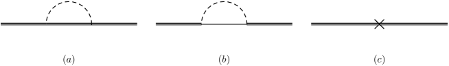
Figure 2: One-loop contributions to the $\Delta$ self-energy at ${\cal O}(p^{3})$.

where the contributions to $s_{\rm 1\,loop}$ of ${\cal O}(p^{3})$ result from the loop diagrams of Fig. 2.

The unrenormalized contribution of Fig. 2 (a) with an internal delta line is given by

$$\Sigma^{\mu\nu}_{{\rm loop},\Delta} = -\frac{5g_{1}^{2}}{3F^{2}}\Biggl{\{}\frac{2}{3}I_{m_{\Delta}}^{\mu\nu}(411)\left(2m_{\Delta}+3\,p/\hskip 1.00006pt-\frac{p^{2}p/\hskip 1.00006pt}{m_{\Delta}^{2}}\right)-g^{\mu\nu}I_{m_{\Delta}}^{\alpha\beta}(411)\left[g_{\alpha\beta}\left(m_{\Delta}+p/\hskip 1.00006pt\right)-2\gamma_{\alpha}p_{\beta}\right]$$ (56)

$$+g^{\mu\nu}I_{m_{\Delta}}^{\alpha\beta\lambda}(411)g_{\alpha\beta}\gamma_{\lambda}-\frac{2}{3}I_{m_{\Delta}}^{\mu\nu\lambda}(411)\frac{{\gamma_{\lambda}}\left({m_{\Delta}}^{2}-p^{2}\right)+2{p_{\lambda}}\left({m_{\Delta}}+p/\hskip 1.00006pt\right)}{m_{\Delta}^{2}}\Biggr{\}}.$$

The corresponding contribution to the pole reads

$$s_{{\rm loop},\Delta} = \frac{5g_{1}^{2}m_{\Delta}^{2}}{10368\pi^{2}F^{2}}\left[40\Lambda^{2}+321{{m_{\Delta}}}^{2}-264{{m_{\Delta}}}^{2}\ln\left(\frac{\Lambda}{{m_{\Delta}}}\right)\right]$$ (57)

$$+\frac{5g_{1}^{2}M^{2}}{864{\pi}^{2}F^{2}}\left[9{m_{\Delta}^{2}}-20\Lambda^{2}m_{\Delta}{c_{1}^{\Delta}}-151{{m_{\Delta}}}^{3}{c_{1}^{\Delta}}-4{m_{\Delta}^{2}}\left(5-22{{m_{\Delta}}}{c_{1}^{\Delta}}\right)\ln\left(\frac{\Lambda}{{m_{\Delta}}}\right)\right]$$

$$+\frac{25g_{1}^{2}}{432\pi F^{2}}M^{3}m_{\Delta}.$$

The unrenormalized one-loop contribution of Fig. 2 (b) with an internal nucleon line is given by

$$\Sigma^{\mu\nu}_{{\rm loop},N}=-\frac{g^{2}}{F^{2}}\left[\left(p/\hskip 1.00006pt+m\right)I^{\mu\nu}_{m}(411)+\gamma_{\lambda}I^{\lambda\mu\nu}_{m}(411)\right].$$ (58)

The corresponding contribution to the pole reads

$$s_{{\rm loop},N} = \frac{g^{2}}{F^{2}}\Biggl{\{}-\frac{35m_{\Delta}^{4}}{768\pi^{2}}-\frac{5m_{\Delta}^{2}\Lambda^{2}}{288\pi^{2}}+\frac{5m_{\Delta}^{4}}{96\pi^{2}}\ln\left(\frac{\Lambda}{m_{\Delta}}\right)$$ (59)

$$+\frac{\delta m_{\Delta}}{96\pi^{2}}\left[20m_{\Delta}^{2}+\Lambda^{2}-20m_{\Delta}^{2}\ln\left(\frac{\Lambda}{m_{\Delta}}\right)\right]$$

$$+\frac{1}{576\pi^{2}}\left[-240\delta^{2}m_{\Delta}^{2}-15m_{\Delta}^{3}\Sigma_{1}^{(0)}-14m_{\Delta}\Sigma_{1}^{(0)}\Lambda^{2}+60m_{\Delta}^{2}\left(2\delta^{2}+M^{2}\right)\ln\left(\frac{\Lambda}{m_{\Delta}}\right)\right]$$

$$-\frac{\delta}{96\pi^{2}}\left[-\Sigma_{1}^{(0)}\Lambda^{2}+6m_{\Delta}(\delta^{2}+M^{2})\ln\left(\frac{\Lambda}{m_{\Delta}}\right)+20m_{\Delta}^{2}\Sigma_{1}^{(0)}\ln\left(\frac{\Lambda}{m_{\Delta}}\right)\right]$$

$$-\frac{m_{\Delta}}{288\pi^{2}}\Biggl{[}-95\delta^{3}+3\delta M^{2}+48\left(\delta^{2}-M^{2}\right)^{\frac{3}{2}}\ln\left(\frac{\delta-\sqrt{\delta^{2}-M^{2}}}{M}\right)$$

$$-48\delta^{3}\ln\left(\frac{M}{m_{\Delta}}\right)+72\delta M^{2}\ln\left(\frac{M}{m_{\Delta}}\right)\Biggr{]}$$

$$-i\frac{m_{\Delta}\left(\delta^{2}-M^{2}\right)^{\frac{3}{2}}}{6\pi}\Biggr{\}},$$

where $\Sigma_{1}^{(0)}=-4c_{1}^{\Delta}\,M^{2}$.

After taking the contribution of the counterterm diagram of Fig. 2 (c) into account, we finally obtain for the pole

$$s=m_{\Delta}^{2}-8m_{\Delta}\,c_{1}^{\Delta}M^{2}+2m_{\Delta}L_{\Delta}+2m_{\Delta}L_{N}-i\,\frac{g^{2}}{F^{2}}\frac{m_{\Delta}\left(\delta^{2}-M^{2}\right)^{\frac{3}{2}}}{6\pi}+{\cal O}(p^{4}),$$ (60)

where

$$L_{\Delta} = -\frac{g^{2}}{576\,\pi^{2}F^{2}}\,\Biggl{[}-95\,\delta^{3}+3\,\delta\,M^{2}\,+48\,\left(\delta^{2}-M^{2}\right)^{\frac{3}{2}}\ln\left(\frac{\delta-\sqrt{\delta^{2}-M^{2}}}{M}\right)$$

$$+24\,\delta\left(3\,M^{2}-2\,\delta^{2}\right)\ln\left(\frac{M}{m_{\Delta}}\right)\Biggr{]},$$

$$L_{N} = \frac{25\,g_{1}^{2}}{864\,\pi\,F^{2}}\,M^{3}.$$

The contribution of the renormalized loop diagrams is indeed of order $p^{3}$ as suggested by the power counting. The so-called pole mass is given by

$${m_{\Delta}}_{\rm pole}=m_{\Delta}-4c_{1}^{\Delta}M^{2}+L_{\Delta}+L_{N}+{\cal O}(p^{4}).$$ (61)

Using the numerical values of Eq. (III) and the SU(6) estimate $g_{1}=9\,g_{A}/5$, we obtain $L_{\Delta}=102.8$ MeV and $L_{N}=15.6$ MeV. We made use of 100 MeV Eidelman:2004wy as the value for $(-2)$ times the imaginary part of the pole to fix $g=1.127$. Unfortunately we do not have a reliable estimate for the parameter $c_{1}^{\Delta}$. For the moment, we assume it to be the same as $\tilde{c}_{1}$ of the $\pi N$ Lagrangian and we obtain an estimate of 126 MeV to 177 MeV for $-4c_{1}^{\Delta}M^{2}$, depending on how $\tilde{c}_{1}$ is fitted to data.

V Summary

We have considered the explicit inclusion of the $\Delta(1232)$ resonance in baryon chiral perturbation theory. The requirement of the consistency of the corresponding effective field theory in the sense of having the right number of degrees of freedom, leads to non-trivial constraints among coupling constants of various interaction terms. These constraints are compatible with the symmetries underlying the effective theory. Implementing them in the effective Lagrangian and using the extended on-mass-shell renormalization scheme (or the reformulated version of the IR renormalization) in combination with the higher-derivative formulation we obtain a consistent effective field theory with a systematic power counting. Thus, we are in a position to calculate low-energy processes involving pions, nucleons, and deltas to any specified order in a small parameter expansion. As applications we have considered the ${\cal O}\left(p^{3}\right)$ contributions to the nucleon mass, the pion-nucleon sigma term, and the pole of the $\Delta$ resonance.

Appendix A Isospin projections

For the isospin components we make use of the following conventions. Let $X=Y\otimes Z$ denote the direct product of isospin-1 and isospin-1/2 spaces, respectively. We parameterize a general vector $|\Psi\rangle\in X$ as

$$|\Psi\rangle=\sum_{i=1}^{3}\sum_{\alpha=-\frac{1}{2}}^{\frac{1}{2}}\Psi_{i,\alpha}|i\rangle\otimes|\frac{1}{2},\alpha\rangle=\sum_{m=-1}^{1}\sum_{\alpha=-\frac{1}{2}}^{\frac{1}{2}}(-)^{m}\Psi^{(1)}_{-m,\alpha}|1,m\rangle\otimes|\frac{1}{2},\alpha\rangle,$$

where the two decompositions refer to a Cartesian and a spherical basis of $Y$, respectively. Using the Clebsch-Gordan decomposition $X=X_{\frac{3}{2}}\oplus X_{\frac{1}{2}}$, we describe a general isospin-3/2 state as

$$X_{\frac{3}{2}}\ni|\Delta\rangle=\sum_{M=-\frac{3}{2}}^{\frac{3}{2}}\Delta_{M}|\frac{3}{2},M\rangle.$$

The scalar product $(\langle 1,m|\otimes\langle\frac{1}{2},\alpha|)|\Delta\rangle$ generates the component $(-)^{m}\Psi_{-m,\alpha}^{(1)}$ of the state $|\Delta\rangle$ in terms of the Clebsch-Gordan coefficient $\langle 1,m;\frac{1}{2},\alpha|(1,\frac{1}{2})\frac{3}{2},M\rangle$ and the components $\Delta_{M}$.

Re-expressing the spherical components in terms of Cartesian components, we then obtain, in terms of the projection operator $\xi^{\frac{3}{2}}$ of Eq. (12),

$$\xi^{\frac{3}{2}}_{1j}\Psi_{\mu,j} = \frac{1}{\sqrt{2}}\,\left(\begin{array}[]{c}\frac{1}{\sqrt{3}}\,\Delta^{0}_{\mu}-\Delta^{++}_{\mu}\\ \Delta^{-}_{\mu}-\frac{1}{\sqrt{3}}\,\Delta^{+}_{\mu}\end{array}\right),$$ (64)

$$\xi^{\frac{3}{2}}_{2j}\Psi_{\mu,j} = -\frac{i}{\sqrt{2}}\,\left(\begin{array}[]{c}\frac{1}{\sqrt{3}}\,\Delta^{0}_{\mu}+\Delta^{++}_{\mu}\\ \Delta^{-}_{\mu}+\frac{1}{\sqrt{3}}\,\Delta^{+}_{\mu}\end{array}\right),$$ (67)

$$\xi^{\frac{3}{2}}_{3j}\Psi_{\mu,j} = \sqrt{\frac{2}{3}}\left(\begin{array}[]{c}\Delta^{+}_{\mu}\\ \Delta^{0}_{\mu}\end{array}\right).$$ (70)

This phase convention agrees with Ref. Tang:1996sq but is opposite to Ref. Hemmert:1997ye .

Appendix B Decomposition

For the decomposition of the dressed propagator and the self-energy of the $\Delta$ resonance of Eqs. (44) and (45) we make use of the basis

$${\cal P}_{1}^{\mu\nu}=g^{\mu\nu},\quad{\cal P}_{2}^{\mu\nu}=\gamma^{\mu}\gamma^{\nu},\quad{\cal P}_{3}^{\mu\nu}=p^{\mu}\gamma^{\nu},\quad{\cal P}_{4}^{\mu\nu}=\gamma^{\mu}p^{\nu},\quad{\cal P}_{5}^{\mu\nu}=p^{\mu}p^{\nu},$$

$${\cal P}_{6}^{\mu\nu}=p/\hskip 1.00006ptg^{\mu\nu},\quad{\cal P}_{7}^{\mu\nu}=p/\hskip 1.00006pt\gamma^{\mu}\gamma^{\nu},\quad{\cal P}_{8}^{\mu\nu}=p/\hskip 1.00006ptp^{\mu}\gamma^{\nu},\quad{\cal P}_{9}^{\mu\nu}=p/\hskip 1.00006pt\gamma^{\mu}p^{\nu},\quad{\cal P}_{10}^{\mu\nu}=p/\hskip 1.00006ptp^{\mu}p^{\nu}.$$ (71)

Appendix C Loop integrals

The loop integrals of Eq. (26) have been calculated using the method of dimensional counting Gegelia:1994zz :

$$I^{\mu\nu}_{m}(411)=g^{\mu\nu}A+\frac{p^{\mu}p^{\nu}}{p^{2}}B,$$ (72)

where

$$A = \frac{1}{192p^{2}\pi^{2}}\,\Biggl{[}m^{4}-2M^{2}m^{2}+3p^{2}m^{2}+M^{4}+3M^{2}p^{2}+p^{2}\Lambda^{2}$$

$$+2M^{2}\left(-m^{2}+M^{2}+p^{2}\right)\ln\left(\frac{M}{m}\right)+2p^{2}\left(-3m^{2}-3M^{2}+p^{2}\right)\ln\left(\frac{\Lambda}{m}\right)\Biggr{]}$$

$$-\frac{I_{f}}{12p^{2}}\left[m^{4}-2\left(M^{2}+p^{2}\right)m^{2}+\left(M^{2}-p^{2}\right)^{2}\right],$$

$$B = -\frac{1}{96p^{2}\pi^{2}}\Biggl{[}2m^{4}-4M^{2}m^{2}-5p^{2}m^{2}+2M^{4}-3(p^{2})^{2}+M^{2}p^{2}$$

$$+4M^{2}\left(-m^{2}+M^{2}+p^{2}\right)\ln\left(\frac{M}{m}\right)+4(p^{2})^{2}\ln\left(\frac{\Lambda}{m}\right)\Biggr{]}$$

$$+\frac{I_{f}}{3p^{2}}\left[m^{4}-2\left(M^{2}+p^{2}\right)m^{2}+M^{4}+(p^{2})^{2}+M^{2}p^{2}\right].$$

$$I^{\mu\nu\rho}_{m}(411)=\frac{g^{\mu\nu}p^{\rho}+g^{\mu\rho}p^{\nu}+g^{\nu\rho}p^{\mu}}{p^{2}}C+\frac{p^{\mu}p^{\nu}p^{\rho}}{(p^{2})^{2}}D,$$ (73)

where

$$C = \frac{1}{4608p^{2}\pi^{2}}\Biggl{\{}12m^{6}-36M^{2}m^{4}-42p^{2}m^{4}+36M^{4}m^{2}-60(p^{2})^{2}m^{2}+24M^{2}p^{2}m^{2}$$

$$-12M^{6}+3(p^{2})^{3}-36M^{2}(p^{2})^{2}+18M^{4}p^{2}-8(p^{2})^{2}\Lambda^{2}$$

$$-24M^{2}\left[m^{4}-2\left(M^{2}+p^{2}\right)m^{2}+M^{4}+(p^{2})^{2}-M^{2}p^{2}\right]\ln\left(\frac{M}{m}\right)$$

$$+24(p^{2})^{2}\left(4\,m^{2}+2\,M^{2}-p^{2}\right)\ln\left(\frac{\Lambda}{m}\right)\Biggr{\}}$$

$$-\frac{I_{f}}{24(p^{2})^{2}}\Biggl{\{}m^{6}-3\left(M^{2}+p^{2}\right)m^{4}+\left[3M^{4}+2p^{2}M^{2}+3(p^{2})^{2}\right]m^{2}$$

$$-\left(M^{2}-p^{2}\right)^{2}\left(M^{2}+p^{2}\right)\Biggr{\}}$$

$$D = \frac{1}{768p^{2}\pi^{2}}\Biggl{\{}-12m^{6}+36M^{2}m^{4}+42p^{2}m^{4}-36M^{4}m^{2}-52(p^{2})^{2}m^{2}$$

$$-48M^{2}p^{2}m^{2}+12M^{6}-19(p^{2})^{2}+4M^{2}(p^{2})^{2}+6M^{4}p^{2}$$

$$+24M^{2}\left[m^{4}-2\left(M^{2}+p^{2}\right)m^{2}+M^{4}+(p^{2})^{2}+M^{2}p^{2}\right]\ln\left(\frac{M}{m}\right)+24(p^{2})^{3}\ln\left(\frac{\Lambda}{m}\right)\Biggr{\}}$$

$$-\frac{I_{f}}{{4p^{2}}}\Biggl{\{}-m^{6}+3\left(M^{2}+p^{2}\right)m^{4}-\left[3M^{4}+4p^{2}M^{2}+3(p^{2})^{2}\right]m^{2}$$

$$+M^{6}+(p^{2})^{3}+M^{2}(p^{2})^{2}+M^{4}p^{2}\Biggr{\}}.$$

In the above expressions $I_{f}$ is given by Fuchs:2003qc

$$I_{f}=\frac{1}{16\pi^{2}}\left[\frac{p^{2}-m^{2}+M^{2}}{p^{2}}\ln\left(\frac{M}{m}\right)+\frac{2\,m\,M}{p^{2}}F(\Omega)\right],$$ (74)

where

$$F(\Omega) = \left\{\begin{array}[]{ll}\sqrt{\Omega^{2}-1}\ln\left(-\Omega-\sqrt{\Omega^{2}-1}\right),&\Omega\leq-1,\\ \sqrt{1-\Omega^{2}}\arccos(-\Omega),&-1\leq\Omega\leq 1,\\ \sqrt{\Omega^{2}-1}\ln\left(\Omega+\sqrt{\Omega^{2}-1}\right)-i\pi\sqrt{\Omega^{2}-1},&1\leq\Omega,\end{array}\right.$$

with

$$\Omega=\frac{p^{2}-m^{2}-M^{2}}{2mM}.$$

References

- (1) S. Weinberg, Physica A96, 327 (1979).
- (2) J. Gasser and H. Leutwyler, Annals Phys. 158, 142 (1984).
- (3) J. Gasser and H. Leutwyler, Nucl. Phys. B250, 465 (1985).
- (4) J. Gasser, M. E. Sainio, and A. Švarc, Nucl. Phys. B307, 779 (1988).
- (5) E. Jenkins and A. V. Manohar, Phys. Lett. B 255, 558 (1991).
- (6) V. Bernard, N. Kaiser, J. Kambor, and U.-G. Meißner, Nucl. Phys. B388, 315 (1992).
- (7) H. Tang, hep-ph/9607436.
- (8) P. J. Ellis and H. Tang, Phys. Rev. C 57, 3356 (1998).
- (9) T. Becher and H. Leutwyler, Eur. Phys. J. C9, 643 (1999).
- (10) J. Gegelia and G. Japaridze, Phys. Rev. D 60, 114038 (1999).
- (11) J. Gegelia, G. Japaridze, and X. Q. Wang, J. Phys. G 29, 2303 (2003).
- (12) T. Fuchs, J. Gegelia, G. Japaridze, and S. Scherer, Phys. Rev. D 68, 056005 (2003).
- (13) T. R. Hemmert, B. R. Holstein, and J. Kambor, J. Phys. G 24, 1831 (1998).
- (14) V. Pascalutsa and D. R. Phillips, Phys. Rev. C 67, 055202 (2003).
- (15) V. Pascalutsa and M. Vanderhaeghen, arXiv:nucl-th/0412113.
- (16) P. A. M. Dirac, Proc. Roy. Soc. Lond. 155A, 447 (1936).
- (17) M. Fierz and W. Pauli, Proc. Roy. Soc. Lond. A 173, 211 (1939).
- (18) K. Johnson and E. C. G. Sudarshan, Annals Phys. 13, 126 (1961).
- (19) G. Velo and D. Zwanziger, Phys. Rev. 186, 1337 (1969).
- (20) L. M. Nath, B. Etemadi, and J. D. Kimel, Phys. Rev. D 3, 2153 (1971).
- (21) H. B. Tang and P. J. Ellis, Phys. Lett. B 387, 9 (1996).
- (22) V. Pascalutsa, Phys. Rev. D 58, 096002 (1998).
- (23) V. Pascalutsa and R. Timmermans, Phys. Rev. C 60, 042201 (1999).
- (24) S. Deser, V. Pascalutsa, and A. Waldron, Phys. Rev. D 62, 105031 (2000).
- (25) V. Pascalutsa, Phys. Lett. B 503, 85 (2001).
- (26) T. Pilling, Mod. Phys. Lett. A 19, 1781 (2004).
- (27) T. Pilling, arXiv:hep-th/0404131.
- (28) D. Djukanovic, M. R. Schindler, J. Gegelia, and S. Scherer, arXiv:hep-ph/0407170.
- (29) M. R. Schindler, J. Gegelia, and S. Scherer, Phys. Lett. B 586, 258 (2004).
- (30) A. Walker-Loud and J. M. S. Wu, arXiv:hep-lat/0504001.
- (31) V. Bernard, T. R. Hemmert, and U.-G. Meißner, arXiv:hep-lat/0503022.
- (32) S. Scherer, in Advances in Nuclear Physics, Vol. 27, edited by J. W. Negele and E. W. Vogt (Kluwer Academic/Plenum Publishers, New York, 2003).
- (33) N. Wies, thesis, Johannes Gutenberg-Universität Mainz, 2005.
- (34) D. Djukanovic, M. R. Schindler, J. Gegelia, G. Japaridze, and S. Scherer, Phys. Rev. Lett. 93, 122002 (2004).
- (35) S. Kamefuchi, L. O’Raifeartaigh, and A. Salam, Nucl. Phys. 28, 529 (1961).
- (36) S. Weinberg, Nucl. Phys. B363, 3 (1991).
- (37) G. Ecker, Prog. Part. Nucl. Phys. 35, 1 (1995).
- (38) Loop diagrams have been calculated using the program FORM Vermaseren:2000nd .
- (39) J. A. M. Vermaseren, arXiv:math-ph/0010025.
- (40) V. Bernard, T. R. Hemmert, and U.-G. Meißner, Phys. Lett. B 565, 137 (2003).
- (41) T. Fuchs, J. Gegelia, and S. Scherer, Eur. Phys. J. A 19, 35 (2004).
- (42) T. Becher and H. Leutwyler, J. High Energy Phys. 0106, 017 (2001).
- (43) R. Koch, Nucl. Phys. A448, 707 (1986).
- (44) J. Gasser, H. Leutwyler, and M. E. Sainio, Phys. Lett. B 253, 252 (1991).
- (45) H. G. A. Hellmann, Z. Phys. 85, 180 (1933).
- (46) R. P. Feynman, Phys. Rev. 56, 340 (1939).
- (47) B. C. Lehnhart, J. Gegelia, and S. Scherer, J. Phys. G 31, 89 (2005).
- (48) P. Buettiker and U.-G. Meißner, Nucl. Phys. A668, 97 (2000).
- (49) M. M. Pavan, I. I. Strakovsky, R. L. Workman, and R. A. Arndt, PiN Newslett. 16, 110 (2002).
- (50) A. E. Kaloshin and V. P. Lomov, Mod. Phys. Lett. A 19, 135 (2004).
- (51) S. Scherer and H. W. Fearing, Phys. Rev. D 52, 6445 (1995).
- (52) S. Eidelman et al. [Particle Data Group], Phys. Lett. B 592, 1 (2004).
- (53) J. Gegelia, G. S. Japaridze, and K. S. Turashvili, Theor. Math. Phys. 101, 1313 (1994).