IFJPAN-V-04-07
CERN-PH-TH/2005-066

Solving constrained Markovian evolution in QCD
with the help of the non-Markovian Monte Carlo^⋆

S. Jadach and M. Skrzypek

Institute of Nuclear Physics, Academy of Sciences,
ul. Radzikowskiego 152, 31-342 Cracow, Poland,
and

CERN Department of Physics, Theory Division
CH-1211 Geneva 23, Switzerland

We present the constrained Monte Carlo (CMC) algorithm for the QCD evolution. The constraint resides in that the total longitudinal energy of the emissions in the MC and in the underlying QCD evolution is predefined (constrained). This CMC implements exactly the full DGLAP evolution of the parton distributions in the hadron with respect to the logarithm of the energy scale. The algorithm of the CMC is referred to as the non-Markovian type. The non-Markovian MC algorithm is defined as the one in which the multiplicity of emissions is chosen randomly as the first variable and not the last one, as in the Markovian MC algorithms. The former case resembles that of the fixed-order matrix element calculations. The CMC algorithm can serve as an alternative to the so-called backward evolution Markovian algorithm of Sjöstrand, which is used for modelling the initial-state parton shower in modern QCD MC event generators. We test practical feasibility and efficiency of our CMC implementation in a series of numerical exercises, comparing its results with those from other MC and non-MC programs, in a wide range of $Q$ and $x$, down to the 0.1% precision level. In particular, satisfactory numerical agreement is found with the results of the Markovian MC program of our own and the other non-MC program. The efficiency of the new constrained MC is found to be quite good.
Keywords: QCD, Monte Carlo, Evolution equations, Markovian process.
PACS numbers: 12.38.Bx, 12.38.Cy 12.39.St

To appear in Computer Physics Communications

IFJPAN-V-04-07
CERN-PH-TH/2005-066

^⋆This work is partly supported by the EU grant MTKD-CT-2004-510126 in partnership with the CERN Physics Department and by the Polish Ministry of Scientific Research and Information Technology grant No 620/E-77/6.PR UE/DIE 188/2005-2008.

1 Introduction

It is commonly known that the evolution equations of the quark and gluon distributions in the hadron, derived in QCD by using the renormalization group or diagrammatic techniques [1], can be often interpreted probabilistically as a Markovian process; see for instance the review of ref. [2].

The Markovian type Monte Carlo (MC) algorithm, implementing the QCD or QED evolution equations, is the basic ingredient in all parton-shower-type MCs. An unconstrained forward Markovian MC, with the evolution kernels from perturbative QCD/QED, can only be used for the final-state radiation (FSR). It is dramatically inefficient for the initial-state radiation (ISR), because the hard process selects certain values of the parton energy and the type of the proton. The MC algorithm that allows us to fix (predefine) the energy and the type of the parton exiting the parton shower, entering the hard process, we shall call the constrained MC algorithm or simply the constrained MC (CMC).

For the ISR parton shower an elegant example of the constrained MC is the backward Markovian evolution MC algorithm of Sjöstrand [4], which is a widely adopted effective solution in all popular MC event generators, notably in PYTHIA [6] and HERWIG [7]. However, the backward Markovian evolution algorithm is a kind of work-around, because it does not solve, strictly speaking, the QCD evolution equations. It merely exploits their solutions coming from an external, typically non-MC, program.

The problem that we are posing and solving in the present work is the following: Is it possible to invent an efficient constrained MC algorithm, not necessarily of the Markovian type, which solves internally the full QCD DGLAP evolution equations on its own, without relying on the external non-MC solutions? Since this is a highly non-trivial technical problem in the area of the MC techniques, it is necessary to clearly state the motivations that have led us to posing it and investing quite some effort in finding at least one satisfactory solution. The most important motivation is that we hope to gain more power in the modelling of the ISR parton showers – this can be potentially profitable for the better integration of the complete next-to-leading-logarithmic (NLL) corrections in the parton shower MCs. We also hope for an easier MC modelling of the unintegrated parton distributions $D_{k}(Q,p_{T},x)$ and MC modelling of the CCFM-type evolution [8] in QCD.

Let us define more precisely the terminology to be used in this work, since it varies in the literature quite a lot. By Markovian MC algorithm we understand an algorithm in which the number of emissions (determining the dimension of the phase-space integral) is generated as the last variable or one of the last ones. On the other hand we shall call a non-Markovian MC algorithm the one in which the number of emissions (the dimension of the integral), is generated randomly as one of the first variables.

The name of “constrained MC” can also be associated with a MC in which the distribution to be generated is restricted to a less-dimensional hyperspace by inserting the $\delta(F(x_{1},...,x_{n}))$ function, where $F(x_{1},...,x_{n})=0$ defines the constraint. The CMC algorithm should efficiently generate points within this subspace. It is widely known that it is usually much more complicated to generate the distribution on such a hyperspace that in the entire space, even if the original unconstrained distribution is simple, for example it is the product of many simple distributions. The energy-momentum conserving $\delta^{(4)}(P-\sum p_{i})$ is a well known example of such a constraint.

In our case the constraint is given by $\delta(x-\prod z_{i})$, where $x$ is predefined (the outermost integration variable, generated in a CMC as the first one) and $z_{i}$ are arguments of the DGLAP evolution kernels. We shall describe an example of the CMC algorithm which fulfills such a constraint, measure its efficiency and make a numerical test of its correctness, by comparing its results with those of the traditional unconstrained Markovian MC, and other non-MC programs.

The outline of the paper is the following: in section 2 we introduce the basic notation and rederive an iterative solution of the DGLAP evolution equations. Since the full solution is algebraically involved, we discuss in section 3 our CMC solution for the simpler case of pure bremsstrahlung out of quark or gluon. Section 4 describes the hierarchical reorganization of the iterative solution, which is necessary for the full scale solution with arbitrary number of gluon–quark transitions. This complete solution, along with numerical tests, is presented in section 5. Summary and outlook concludes the paper. For the sake of completeness, a small appendix lists the standard LL QCD kernels.

This paper describes the main part of a wider effort on the MC modelling of the QCD evolution equations. In ref. [9] the reader may find an alternative CMC algorithm for the QCD evolution, which looks slightly inferior to the one presented here and is implemented numerically only for pure bremsstrahlung. References [10] and [11] are devoted to a precision MC modelling of the LL and NLL DGLAP evolution equations using the Markovian (unconstrained) class of algorithms. In this context it is worth to remind the reader that the consistent integration of the NLL perturbative corrections at the fully exclusive level in the MC event generator of the parton shower type is the challenging problem both theoretically and practically. For the recent efforts in this direction see refs. [12, 13], for example. The algebraic proof of certain important identity used in this work is published separately in ref. [14].

2 Iterative solution of the QCD evolution equations

Let us rederive the iterative solution of the QCD evolution equations. The starting point is the DGLAP [1] set of evolution equations:

$$\begin{split}\frac{\partial}{\partial t}D_{k}(t,x)&=\sum_{j}\int\limits_{x}^{1}\frac{dz}{z}P_{kj}(z)\frac{\alpha_{S}(t)}{\pi}D_{j}\Big{(}t,\frac{x}{z}\Big{)}=\sum_{j}{\mathcal{P}}_{kj}(t,\cdot)\otimes D_{j}(t,\cdot),\end{split}$$ (1)

where

$$f(\cdot){\otimes}g(\cdot)(x)\equiv\int dx_{1}dx_{2}\delta(x-x_{1}x_{2})f(x_{1})g(x_{2}),$$ (2)

and ${\mathcal{P}}_{kj}(t,z)\equiv\frac{\alpha_{S}(t)}{\pi}P_{kj}(z)$. Indices $i$ and $k=G,q,\bar{q}$ denote gluon or quark – the evolution time is $t=\ln(Q)$. The differential evolution equation can be turned into the following integral equation:

$$\begin{split}&e^{\Phi_{k}(t,t_{0})}D_{k}(t,x)=D_{k}(t_{0},x)+\int\limits_{t_{0}}^{t}dt_{1}e^{\Phi_{k}(t_{1},t_{0})}\sum_{j}{\mathcal{P}^{\Theta}_{kj}(t_{1},\cdot)}\otimes D_{j}(t_{1},\cdot)(x),\end{split}$$ (3)

where $\varepsilon$ is the IR regulator in the kernels,

$${\mathcal{P}_{kj}(t,z)} = -\mathcal{P}^{\delta}_{kk}(t,\varepsilon)\delta_{kj}\delta(1-z)+\mathcal{P}^{\Theta}_{kj}(t,z),$$ (4)

$$\mathcal{P}^{\Theta}_{kj}(t,z) = \mathcal{P}_{kj}(t,z)\Theta(1-z-\varepsilon),$$ (5)

and the Sudakov form factor is given by

$${\Phi_{k}(t,t_{0})}=\int_{t_{0}}^{t}dt^{\prime}\;\mathcal{P}^{\delta}_{kk}(t^{\prime},\varepsilon).$$ (6)

The complete set of LL kernels $\mathcal{P}_{kj}$ is collected in an appendix.

The multiple iteration of the above integral equation leads us to an iterative solution of the evolution equations, given by the following series of integrals, ready for the evaluation with the help of the standard MC methods:

$$\begin{split}&D_{k}(t,x)=e^{-\Phi_{k}(t,t_{0})}D_{k}(t_{0},x)+\sum_{n=1}^{\infty}\;\sum_{k_{0}...k_{n-1}}\bigg{[}\prod_{i=1}^{n}\int\limits_{t_{0}}^{t}dt_{i}\;\Theta(t_{i}-t_{i-1})\int\limits_{0}^{1}dz_{i}\bigg{]}\\ &e^{-\Phi_{k}(t,t_{n})}\int\limits_{0}^{1}dx_{0}\;\bigg{[}\prod_{i=1}^{n}\mathcal{P}_{k_{i}k_{i-1}}^{\Theta}(t_{i},z_{i})e^{-\Phi_{k_{i-1}}(t_{i},t_{i-1})}\bigg{]}D_{k_{0}}(t_{0},x_{0})\delta\bigg{(}x-x_{0}\prod_{i=1}^{n}z_{i}\bigg{)},\end{split}$$ (7)

where $k_{n}\equiv k$. In ref. [10] the above equation was solved with the three-digit precision using the Markovian MC method. In this work the above solution is the starting point for constructing the CMC algorithm.

There is still one standard technical point: the one-loop dependence of the strong coupling $\alpha_{S}(t)=2\pi/(\beta_{0}(t-\ln\Lambda_{0}))$ may destroy the efficiency of the MC algorithm, unless it is conveniently compensated by means of the mapping $t_{i}\to\tau_{i}=\ln(t_{i}-\ln\Lambda_{0})$. Once it is done, the iterative solution transforms into the following form:

$$\begin{split}D_{k}&(\tau,x)=e^{-\Phi_{k}(\tau,\tau_{0})}D_{k}(\tau_{0},x)+\sum_{n=1}^{\infty}\;\int_{0}^{1}dx_{0}\;\sum_{k_{0}...k_{n-1}}\bigg{[}\prod_{i=1}^{n}\int_{\tau_{0}}^{\tau}d\tau_{i}\;\Theta(\tau_{i}-\tau_{i-1})\int_{0}^{1}dz_{i}\bigg{]}\\ &~{}~{}\times e^{-\Phi_{k}(\tau,\tau_{n})}\bigg{[}\prod_{i=1}^{n}\mathcal{P}_{k_{i}k_{i-1}}^{\Theta}(\tau_{i},z_{i})e^{-\Phi_{k_{i-1}}(\tau_{i},\tau_{i-1})}\bigg{]}D_{k_{0}}(\tau_{0},x_{0})\delta\bigg{(}x-x_{0}\prod_{i=1}^{n}z_{i}\bigg{)},\end{split}$$ (8)

where $k\equiv k_{n}$. The kernel $\mathcal{P}$ and form factor $\Phi$ are from now on redefined as follows:

$$\begin{split}\mathcal{P}_{k_{i}k_{i-1}}(\tau_{i},z_{i})&=\frac{\alpha_{S}(t)}{\pi}\;\frac{\partial t}{\partial\tau}\;P_{k_{i}k_{i-1}}(z_{i})=\frac{2}{\beta_{0}}\;P_{k_{i}k_{i-1}}(z_{i}),\\ {\Phi_{k}(\tau,\tau_{0})}&=\int_{\tau_{0}}^{\tau}d\tau^{\prime}\;\mathcal{P}^{\delta}_{kk}(\varepsilon)=(\tau-\tau_{0})\mathcal{P}^{\delta}_{kk}(\varepsilon).\end{split}$$ (9)

In the present LL case, $\mathcal{P}$ becomes completely independent of $\tau_{i}$. See also refs. [9, 11] for more discussion on the optimal choice of the evolution time.

In the following we shall often employ the short-hand notation:

$$\begin{split}&\theta_{x>y}\equiv\theta(x-y),\;\;\hbox{where}\;\;\theta_{x>y}=1\;\;\hbox{for}\;\;x>y,\;\;\hbox{otherwise}\;\;\theta_{x>y}=0,\\ &\delta_{x=y}\;\;\hbox{instead of}\;\;\delta(x-y),\end{split}$$ (10)

so as to keep formulas more compact.

Throughout this work we concentrate on the LL case. However, our CMC algorithm solves most of the problems on the way to the CMC solution for the NLL DGLAP. The exact Monte Carlo solution of the NLL DGLAP evolution equations in the framework of the unconstrained Markovian approach is presented in a separate work (ref. [11]). It may serve as a numerical benchmark for the future work on the NLL CMC.

3 CMC for pure bremsstrahlung only

Before we unfold all the details of our construction of the CMC algorithm for the full DGLAP equations, let us first describe it for the simpler case of the pure QCD bremsstrahlung. This will help the reader to follow all algebraic technicalities of the full CMC solution. It will also provide a building block for the full CMC solution.

The starting point is the iterative solution of the QCD evolution equations of eq. (8) truncated to the multiple gluon bremsstrahlung emitted from the parton $k=G,q,\bar{q}$, with the starting distribution $D_{k}(\tau_{0},x_{0})=\delta(x_{0}-1)$:

$$\begin{split}&x\mathcal{D}_{kk}(\tau,\tau_{0};x)=e^{-\Phi_{k}(\tau,\tau_{0})}\bigg{\{}\delta_{x=1}+\sum_{n=1}^{\infty}\frac{1}{n!}\;\prod_{i=1}^{n}\int\limits_{\tau_{i-1}}^{\tau}d\tau_{i}\;\int\limits_{0}^{1}dz_{i}\;z_{i}\mathcal{P}_{kk}^{\Theta}(\tau_{i},z_{i})\delta_{x=\prod_{i=1}^{n}z_{i}}\bigg{\}}.\\ \end{split}$$ (11)

For the purpose of the MC generation, we introduce simplified kernels:

$$\begin{split}&zP^{\Theta}_{GG}(z)\to z\hat{P}^{\Theta}_{GG}(z)=zB_{GG}\Theta(1-\varepsilon-z)\left(\frac{1}{1-z}+\frac{1}{z}\right)=B_{GG}\frac{\Theta(1-\varepsilon-z)}{1-z},\\ &zP^{\Theta}_{qq}(z)\to z\hat{P}^{\Theta}_{qq}(z)=B_{qq}\frac{\Theta(1-\varepsilon-z)}{1-z}.\end{split}$$ (12)

Note that in eq. (12) we do not modify the virtual parts of the kernels. We also do not assume any sum rules relating $\mathcal{P}^{\delta}_{kk}$ to $\int z\mathcal{P}^{\theta}_{kk}$. This is so because we view eq. (11) as a part of a bigger framework (eq. (8) for example) with both quarks and gluons, and we will assume later on a complete sum rule $\mathcal{P}^{\delta}_{kk}=\sum_{j}\int z\mathcal{P}^{\theta}_{jk}$.

The above simplification of eq. (12) will be countered by the MC weight $w_{P}$ defined below:

$$\begin{split}&x\mathcal{D}_{kk}(\tau,\tau_{0};x)=e^{-\Phi_{k}(\tau,\tau_{0})}\bigg{\{}\delta_{x=1}+x^{\omega_{k}}\sum_{n=1}^{\infty}\frac{1}{n!}b_{k}^{n}\;\prod_{i=1}^{n}\int\limits_{\ln(\varepsilon)}^{\ln(1-x)}dy_{i}\;\delta_{x=\prod_{i=1}^{n}z_{i}(y_{i})}\int\limits_{\tau_{i-1}}^{\tau}d\tau_{i}\;w_{P}\bigg{\}},\end{split}$$ (13)

where $y_{i}=\ln(1-z_{i})$ and

$$\begin{split}&w_{P}=x^{-\omega_{k}}\prod_{j=1}^{n}\frac{P^{\Theta}_{kk}(z_{j})}{\hat{P}^{\Theta}_{kk}(z_{j})},\\ &\Phi_{k}(\tau,\tau_{0})=(\tau-\tau_{0})\left(b_{k}\ln\frac{1}{\varepsilon}-a_{k}\right),\\ &b_{k}\equiv\frac{2}{\beta_{0}}B_{kk},\quad a_{k}\equiv\frac{2}{\beta_{0}}A_{kk}.\end{split}$$ (14)

The factor $x^{\omega_{k}}$ is introduced in order to obtain as uniform shape of the MC weight distribution for all $x\in(0,1)$ as possible. It will also help to correct for the fact that $P_{qq}(z_{i})$ does not have a $1/z_{i}$ component – in this case $\prod_{i}z_{i}=x$ can be pulled out of the integrand. For the moment we assume $\omega_{G}=0$ and $\omega_{q}=1$, but obviously they are dummy parameters, which may influence the MC efficiency but not the final MC distributions.

The energy constraint

$$\begin{split}&x=\prod_{i=1}^{n}z_{i}(y_{i})=\prod_{i=1}^{n}\big{(}1-\exp(y_{i})\big{)}=F(y_{1},y_{2},\dots,y_{n}),\equiv F({\bf y})\quad\hbox{\rm or}\\ &\ln\frac{1}{x}=\sum_{j=1}^{n}f(y_{j})=-\ln F({\bf y});\quad f(y_{j})=-\ln\big{(}1-\exp\big{(}y_{j})\big{)}=-\ln z_{j}\end{split}$$ (15)

provides also an integration limit $z(y_{i})\geq x$, which translates into $y_{i}=\ln(1-z_{i})\leq\ln(1-x)$. Taking advantage of the symmetry of the integrand we can introduce ordering in the $y$-variables:

$$\begin{split}&x\mathcal{D}_{kk}(\tau,\tau_{0};x)=e^{-\Phi_{k}(\tau,\tau_{0})}\bigg{\{}\delta_{x=1}+\\ &~{}~{}~{}+x^{\omega_{k}-1}\sum_{n=1}^{\infty}b_{k}^{n}\;\prod_{i=1}^{n}\int\limits_{y_{\min}}^{y_{\max}}dy_{i}\;\theta_{y_{i}>y_{i-1}}\delta\left(\ln\frac{1}{x}-\sum_{j}f(y_{j})\right)\int\limits_{\tau_{0}}^{\tau}d\tau_{i}\;w_{P}\bigg{\}}.\;\end{split}$$ (16)

where $y_{0}\equiv y_{\min}=\ln(\varepsilon)$ and $y_{\max}=\ln(1-x)$.

The function $f(y_{i})$ is very steeply (exponentially) rising, hence the constraint $x=\prod_{i=1}^{n}z_{i}(y_{i})$ is effectively “saturated” by a single $z_{j}$ while the other ones are $z_{i}\simeq 1,\;i\neq j$. In terms of $y$ variables, $y_{j}\simeq y_{\max}$, while the other ones $y_{i},\;\;i\neq j$, move freely within the $(y_{\min},y_{\max})$ interval. In our case, because we ordered $y$-variables, it is the biggest $y_{n}\simeq y_{\max}$ that effectively takes responsibility for satisfying the constraint.

In the following we translate the above statements into rigorous mathematics. The procedure of eliminating the energy constraint goes in three steps:
Step one. We introduce the new integration variable $Y$. Its introduction is immediately countered by the $\delta$-function:

$$\begin{split}&x\mathcal{D}_{kk}(\tau,\tau_{0};x)=e^{-\Phi_{k}(\tau,\tau_{0})}\bigg{\{}\delta_{x=1}+x^{\omega_{k}-1}\sum_{n=1}^{\infty}b_{k}^{n}\;\\ &~{}~{}~{}\times\int dY\prod_{i=1}^{n}\int\limits_{y_{\min}}^{y_{\max}}dy_{i}\;\theta_{y_{i}>y_{i-1}}\delta(y_{n}+Y-y_{\max})\delta\left(\ln\frac{1}{x}-\sum_{j}f(y_{j})\right)\int\limits_{\tau_{0}}^{\tau}d\tau_{i}\;w_{P}.\bigg{\}}.\;\end{split}$$ (17)

Step two. We perform the following simple linear transformation

$$y_{i}=y^{\prime}_{i}-Y.$$ (18)

Note that $Y$ was “adjusted” from the very beginning such that $y^{\prime}_{n}=y_{n}+Y=y_{\max}$, see also a graphical illustration in fig. 1.

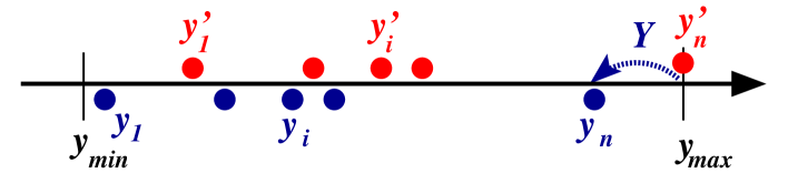
Figure 1: Graphical representation of the linear transformation $y_{i}\to y_{i}^{\prime}$

The Jacobian of the above linear transformation is equal to 1. We obtain:

$$\begin{split}&x\mathcal{D}_{kk}(\tau,\tau_{0};x)=e^{-\Phi_{k}(\tau,\tau_{0})}\bigg{\{}\delta_{x=1}+x^{\omega_{k}-1}\sum_{n=1}^{\infty}b_{k}^{n}\;\int dY\\ &~{}~{}~{}~{}~{}~{}~{}~{}\times\prod_{i=1}^{n}\int\limits_{y_{\min}}^{y_{\max}}dy^{\prime}_{i}\;\theta_{y^{\prime}_{i}>y^{\prime}_{i-1}}\delta(y^{\prime}_{n}-y_{\max})\delta\left(\ln\frac{1}{x}-\sum_{j}f(y^{\prime}_{j}-Y)\right)\int\limits_{\tau_{0}}^{\tau}d\tau_{i}\;w_{P}\bigg{\}},\end{split}$$ (19)

where $y^{\prime}_{0}\equiv y_{\min}+Y$, and $\theta_{y_{1}>y_{\min}}=\theta_{y^{\prime}_{1}>Y+y_{\min}}=\theta_{y^{\prime}_{1}>y^{\prime}_{0}}$ defines the IR lower boundary of the phase space.
Step three. The energy constraint $\delta(x-F)$ is eliminated by means of the $Y$-integration:

$$\begin{split}&x\mathcal{D}_{kk}(\tau,\tau_{0};x)=e^{-\Phi_{k}(\tau,\tau_{0})}\bigg{\{}\delta_{x=1}+\\ &~{}~{}~{}+x^{\omega_{k}-1}\sum_{n=1}^{\infty}b_{k}^{n}\;\prod_{i=1}^{n}\int\limits_{y_{\min}}^{y_{\max}}dy^{\prime}_{i}\;\theta_{y^{\prime}_{i}>y^{\prime}_{i-1}}\delta(y^{\prime}_{n}-y_{\max})\frac{1}{|\partial_{Y}\ln F({\bf y}^{\prime}-Y)|_{Y=Y_{0}}}\int\limits_{\tau_{0}}^{\tau}d\tau_{i}\;w_{P}\bigg{\}},\end{split}$$ (20)

where $Y_{0}=Y_{0}(x,{\bf y}^{\prime})$ is the solution of the transcendental equation $x=F({\bf y}^{\prime}-Y)$. One subtle point is that thanks to $y^{\prime}_{0}=y_{\min}+Y_{0}(x,{\bf y}^{\prime})$, and $Y_{0}\geq 0$ we may keep formally the same integration limits $y^{\prime}_{i}\in(y_{\min},y_{\max})$ as before.

Summarizing the above three steps: we effectively traded complicated $\delta(x-F({\bf y}))$ into much simpler $\delta(y^{\prime}_{n}-y_{\max})$. We may also say that we projected, by means of the parallel shift (along the diagonal), points from the hyperspace $y_{n}=y_{\max}$ into the hyperspace $x=F({\bf y})$.

Let us now have a closer look into formula for $\partial_{Y}F({\bf y}^{\prime}-Y)$, which is necessary for the MC weight and for the numerical solution of the equation $x=F({\bf y}^{\prime}-Y)$:

$$\begin{split}&|\partial_{Y}\ln F({\bf y}^{\prime}-Y)|_{Y=Y_{0}}=\left|\left(\sum_{k=1}^{n}\partial_{Y}f(y_{k}^{\prime}-Y)\right)\right|_{Y=Y_{0}}=\bigg{|}\sum_{k=1}^{n}\frac{\exp(y_{k}^{\prime}-Y)}{z_{k}}\bigg{|}_{Y=Y_{0}}\\ &=\sum_{k=1}^{n}\frac{1-z_{k}}{z_{k}}\;=\sum_{k=1}^{n}|\partial_{y}\ln z(y)|_{z=z_{k}}\end{split}$$ (21)

The additional transformation $y^{\prime}_{i}=y_{\min}+r_{i}\Delta_{y}$ with $\Delta_{y}=y_{\max}-y_{\min}$ and $0\leq r_{i}\leq 1$ as well as exporting part of the integrand into MC weight brings the integral closer to the form suited for the MC generation:

$$\begin{split}&x\mathcal{D}_{kk}(\tau,\tau_{0};x)=e^{-\Phi_{k}(\tau,\tau_{0})}\bigg{\{}\delta_{x=1}+x^{\omega_{k}-1}\sum_{n=1}^{\infty}b_{k}^{n}\Delta^{n-1}_{y}\prod_{i=1}^{n}\int\limits_{0}^{1}dr_{i}\;\theta_{r_{i}>r_{i-1}}\delta(r_{n}-1)\int\limits_{\tau_{0}}^{\tau}d\tau_{i}w_{0}^{\#}\bigg{\}},\\ &w_{0}^{\#}=w_{P}\frac{1}{|\partial_{Y}\ln F({\bf y}^{\prime}-Y)|_{Y=Y_{0}}}\;\theta_{y^{\prime}_{1}-Y_{0}>y_{\min}},\quad r_{0}\equiv 0.\end{split}$$ (22)

The average or maximum weight is improved if the weight $w_{0}^{\#}(z_{1},...,z_{n})$ is rescaled by the function $g(x)$ (which can be pulled out of the integral). The weight distribution is conveniently stabilized if we take for $g(x)$ the biggest term in $|\partial_{y}\ln z(y)|_{z=z_{k}}$, with the largest $y_{k}$, which we approximate as $z_{k}\simeq x$:

$$\begin{split}&w^{\#}=w_{P}\;\frac{xg(x)}{|\partial_{Y}\ln F({\bf y}^{\prime}-Y)|_{Y=Y_{0}}}\;\theta_{y^{\prime}_{1}-Y_{0}>y_{\min}},\quad g(x)=|\partial_{y}\ln z(y)|_{z=x}=\frac{1-x}{x}.\end{split}$$ (23)

Finally we introduce the normalized variables $s_{i}=(\tau_{i}-\tau_{0})/(\tau-\tau_{0})$, rescale $w^{\#}$ and symmetrize over $r_{i}$:

$$\begin{split}&x\mathcal{D}_{kk}(\tau,\tau_{0};x)=e^{-\Phi_{k}(\tau,\tau_{0})}\bigg{\{}\delta_{x=1}+\\ &~{}~{}~{}~{}~{}~{}~{}~{}~{}~{}+\frac{x^{\omega_{k}-1}}{xg(x)}\sum_{n=1}^{\infty}b_{k}\frac{\Delta^{n-1}}{(n-1)!}\;(\tau-\tau_{0})\prod_{i=1}^{n}\int\limits_{0}^{1}dr_{i}\;\frac{\delta(1-\max r_{j})}{n}\int\limits_{0}^{1}ds_{i}\;w^{\#}\bigg{\}},\\ &\Delta=b_{k}(\tau-\tau_{0})\Delta_{y}=b_{k}(\tau-\tau_{0})[\ln(1-x)-\ln\varepsilon]=\mathcal{R}(1-x)-\mathcal{R}(\varepsilon),\;\\ &\mathcal{R}(x)=b_{k}(\tau-\tau_{0})\ln x.\end{split}$$ (24)

Introducing explicitly a Poisson distribution $P(n|\lambda)=e^{-\lambda}\lambda^{n}/n!$, and remembering that $\Phi_{k}(\tau,\tau_{0})=-(b_{k}\ln\varepsilon+a_{k})(\tau-\tau_{0})$, we obtain the following master formula on which the MC algorithm is built:

$$\begin{split}&x\mathcal{D}_{kk}(\tau,\tau_{0};x)=\sum_{n=0}^{\infty}e^{(\tau-\tau_{0})a_{k}}\bigg{\{}e^{\mathcal{R}(\varepsilon)}\delta_{n=0}\delta_{x=1}+\delta_{n>0}\theta_{1-x>\varepsilon}e^{\mathcal{R}(1-x)}\frac{b_{k}x^{\omega_{k}-1}}{xg(x)}(\tau-\tau_{0})\\ &~{}~{}~{}~{}~{}~{}~{}~{}~{}~{}\times P\Big{(}n-1\Big{|}\mathcal{R}(1-x)-\mathcal{R}(\varepsilon)\Big{)}\prod_{i=1}^{n}\int\limits_{0}^{1}dr_{i}\;\frac{\delta(1-\max r_{j})}{n}\int\limits_{0}^{1}ds_{i}\;w^{\#}\bigg{\}},\\ &\tau_{i}=\tau_{0}+s_{i}(\tau-\tau_{0}),\quad z_{i}=1-e^{y_{i}}=1-\exp(y_{\min}+r_{i}\Delta_{y}-Y_{0}).\end{split}$$ (25)

In our CMC algorithm for pure bremsstrahlung one generates first $x$, then $n$, next $z_{i}$ (constructed from $y_{i}$) and finally $\tau_{i}$ (constructed from $s_{i}$). The algorithm is clearly non-Markovian, as is seen from the fact that the number of emissions is generated as the second variable, not as the last one. The distribution of the variable $x$ is done according to the following primary distribution:

$$\begin{split}x\mathcal{D}^{\prime}_{kk}(\tau,\tau_{0};x)&=e^{(\tau-\tau_{0})a_{k}}\bigg{\{}\delta_{x=1}\;e^{\mathcal{R}(\varepsilon)}+\theta_{1-x>\varepsilon}e^{\mathcal{R}(1-x)}\;\frac{b_{k}(\tau-\tau_{0})}{xg(x)}\;x^{\omega_{k}-1}\bigg{\}}\\ &=e^{(\tau-\tau_{0})a_{k}}\bigg{\{}\delta_{x=1}\;e^{\mathcal{R}(\varepsilon)}+\theta_{1-x>\varepsilon}\;e^{\mathcal{R}(1-x)}|\partial_{x}\mathcal{R}(1-x)|\;x^{\omega_{k}-1}\bigg{\}},\end{split}$$ (26)

which is obtained by means of neglecting $w^{\#}$ and performing all summations and integrations. The MC weight $w^{\#}$ is, of course, restored later on.

It is quite convenient, in the construction of the MC program, that in the above distribution we are able to extend artificially the integration above $x=1-\varepsilon$, by means of mapping $x$ into the new variable $U=\exp(\mathcal{R}(1-x))$, so that we can generate $x$ as if there was no $\delta_{x=1}$. This resembles quite strongly the analogous trick for the multiple photon emissions in the YFS-type MCs for QED [18]. Let us work out the details, restoring the initial parton distribution at $t=t_{0}$ and the hard process function $H(x)$:

$$\begin{split}&\int\limits_{\epsilon_{1}}^{1}dx\;H(x)\;D_{kk}(\tau,x)=\int\limits_{\epsilon_{1}}^{1}dx\;\int\limits_{0}^{1}dZ\;\int\limits_{0}^{1}dx_{0}\;\delta(x-x_{0}Z\;)H(x)\;\mathcal{D}^{\prime}_{kk}(\tau,\tau_{0};Z)\;D_{k}(\tau_{0},x_{0})\;\\ &=\int\limits_{\epsilon_{1}}^{1}dxH(x)\int\limits_{x}^{1}\frac{dZ}{Z}Z^{\omega_{k}-2}e^{(\tau-\tau_{0})a_{k}}\left\{\delta_{Z=1}\;e^{\mathcal{R}(\varepsilon)}+\theta_{1-Z>\varepsilon}e^{\mathcal{R}(1-Z)}|\partial_{Z}\mathcal{R}(1-Z)|\right\}D_{k}\Big{(}\tau_{0},\frac{x}{Z}\Big{)}\\ &=\int\limits_{\epsilon_{1}}^{1}dx\;H(x)\int\limits_{0}^{\exp(\mathcal{R}(1-x))}\!\!\!dU\;Z(U)^{\omega_{k}-3}e^{(\tau-\tau_{0})a_{k}}\left\{\delta_{U=0}\;e^{\mathcal{R}(\varepsilon)}+\theta_{U\geq\exp(\mathcal{R}(\varepsilon))}\right\}D_{k}\Big{(}\tau_{0},\frac{x}{Z(U)}\Big{)}\\ &~{}~{}=\int\limits_{\epsilon_{1}}^{1}\frac{dx}{x}\;H(x)\;\int\limits_{0}^{\exp(\mathcal{R}(1-x))}\!\!\!dU\;Z(U)^{\omega_{k}-2}e^{(\tau-\tau_{0})a_{k}}\;\;\frac{x}{Z(U)}D_{k}\Big{(}\tau_{0},\frac{x}{Z(U)}\Big{)},\\ &U(Z)=e^{\mathcal{R}(1-Z)}=(1-Z)^{b_{k}(\tau-\tau_{0})},\\ &Z(U)=1-\exp\big{(}(b_{k}(\tau-\tau_{0}))^{-1}\ln U\big{)},\end{split}$$ (27)

and remembering that $1>Z(U)>1-\varepsilon$ is mapped exactly into one point at $U=0$, reproducing the component $\sim\delta_{Z=1}$, i.e. $\int^{\exp(\mathcal{R}(\varepsilon))}_{0}dU=\exp(\mathcal{R}(\varepsilon))$. Once $x$ is chosen, $n$ is generated according to a Poisson distribution (shifted by 1) and then all variables $\tau_{i}$ and $z_{i}$ are generated.

The above collection of detailed formulas determines uniquely the whole CMC algorithm for the pure bremsstrahlung case. For the sake of completeness let us summarize point by point the complete CMC algorithm:

• The outmost integration variable generated as the first one is total $x$, the argument of the hard process cross section $H(x)$.

• The second generated variable is $Z$, the total loss of energy due to multiple gluon bremsstrahlung, with the help of the mapping: $U(Z)=e^{\mathcal{R}(1-Z)}=(1-Z)^{b_{k}(\tau-\tau_{0})}$.

• The generation of variables $x$ and $U$ (and of $k=k_{0}$, if necessary) is done with the help of the general-purpose MC tool FOAM [19, 20].

• Knowing $Z(U)$, if $Z>1-\varepsilon$, the emission multiplicity $n$ is generated according to a Poisson distribution $P_{n-1}$ (non-Markovian!), otherwise $Z=1$ and $n=0$.

• Variables $s_{i},i=1,2,...,n$ are generated uniformly and mapped onto $\tau_{i}(s_{i})$ and $t_{i}(\tau_{i})$. They are ordered.

• Not ordered variables $r_{i}\in(0,1)$ are generated, such that one of them is set equal to 1; they are mapped into $y^{\prime}_{i}(r_{i})$.

• The solution $Y=Y_{0}$ of the transcendental equation $\ln F({\bf y}^{\prime}-Y)-\ln x=0$ is found numerically (NB: the derivative $\partial_{Y}\ln F$ for the MC weight is obtained as a byproduct).

• With $Y_{0}$ at hand, all variables $z_{i}(y_{i}(y^{\prime}_{i})),\;i=1,2,...,n$ are calculated.

• In the case $y_{1}<y_{\min}$, see fig. 2, the MC weight $w^{\#}$ is zero and the algorithm stops.

• Finally the MC weight $w^{\#}$ is calculated. Optionally the weighted MC event is transformed into an unweighted one with the help of the standard rejection method.

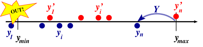
Figure 2: Graphical representation of the rescaling procedure $y_{i}\to y_{i}^{\prime}$

In this way we completed the description of the CMC algorithm for the pure bremsstrahlung case, which will be the essential building block for the general-case CMC algorithm described in the following.

3.1 Numerical test of the CMC for pure bremsstrahlung

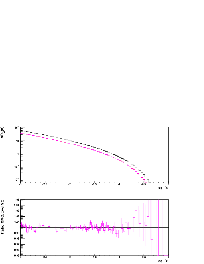
Figure 3: Comparison of CMC and EvolMC in the case of pure bremsstrahlung out of gluon.

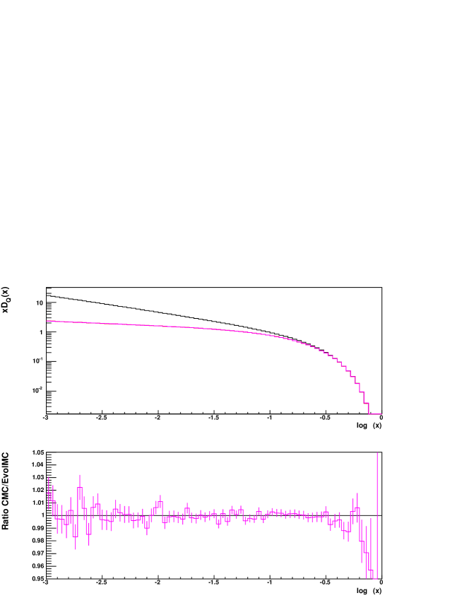
Figure 4: Comparison of CMC and EvolMC in the case of pure bremsstrahlung out of quark

The CMC for pure gluon bremsstrahlung was tested separately for emission from gluon and quark lines by comparing its results with those from the Markovian MC EvolMC of refs. [10] and [11]. As in ref. [10] results are for the LL DGLAP evolution of the parton distribution in the proton from energy scale $Q=1$ GeV to $Q=1$ TeV. We use the same starting parton distributions in proton at $Q=1$ GeV as in ref. [10] and the same range of $x\in(0.001,1)$. In the upper plot of fig. 3 we show the gluon distribution evolved up to scale $Q=1$ TeV (lower curve) due to pure gluon bremsstrahlung, obtained using our new CMC and the Markovian EvolMC. Results are indistinguishable; we therefore plot their ratio in the lower plot of this figure. The results of the two programs agree perfectly, within the statistical errors, which are of order $0.5\%$ at low $x$. MC results are for statistics of a few hundred millions of MC events. A higher-statistics comparison will be presented in the following section. We also include, in the upper plot of fig. 3, the result of the evolution (from the Markovian MC) due to all transitions, not only bremsstrahlung. As we see, the complete result differs from the pure bremsstrahlung one by a factor of almost 2, hence the inclusion of the transitions of gluon into quark and back is very important.

In fig. 4 we present numerical results of the analogous comparisons for the quark singlet $Q=q+\bar{q}$. Again, pure bremsstrahlung results of the new CMC agree very well with these of the Markovian EvolMC, to within of the statistical error, which is about 0.5% in most of the $x$ range. Contrary to the previous case the curve for full evolution coincides with that for pure bremsstrahlung. This is easy to explain as a result of the suppression of the gluon distribution at high $x$, resulting in the smallness of the $Q\leftarrow G$ contribution.

On the technical side, let us remark that there are two methods of obtaining pure bremsstrahlung contributions from the Markovian MC. One may simulate full DGLAP evolution, including $Q\leftrightarrow G$ transitions and select events (evolution histories) in which only pure bremsstrahlung occurs. The other method is to suppress kernels for $Q\leftrightarrow G$ transitions completely. In the present version of the Markovian EvolMC, both methods are available, and both give identical results. In the present work we mainly use the first method of selecting evolution histories out of complete evolution.

4 The CMC with the flavour transitions – full DGLAP

4.1 General discussion

Before getting into details, let us describe the essential ingredients of our CMC algorithm for full LL DGLAP, with an arbitrary number of flavour-changing transitions $G\leftrightarrow Q$, where $Q=q,\bar{q}$. The first ingredient is the observation, made in ref. [10], that the average number $\langle n\rangle$ of $G\leftrightarrow Q$ transitions is much lower than the average number $\langle N\rangle$ of $G\to G$ or $Q\to Q$ ones, that is of the gluon bremsstrahlung emissions. In fact $\langle n\rangle\simeq 1$ for the evolution from $Q_{0}=1$ GeV to $Q=1$ TeV, while $\langle N\rangle\sim 20$ (for $\varepsilon=10^{-4}$). This suggests quite strongly that we should consider the evolution process (emission chain) as a two-level process: sublevel of the pure bremsstrahlung and superlevel of the flavour transitions. Let us call it “hierarchical” organization of the emission chain. The hope is that the small number of superlevel transitions can be modelled, for example by a general-purpose MC tool such as FOAM, thanks to a relatively small dimensionality of the problem. The assumption is that pure bremsstrahlung segments can be treated separately and efficiently.

As discussed in ref. [9], for the treatment of the energy constraint $\delta$-function, there are at least two options. We may deal with it independently and separately for each of the two levels; this is called type I solution in ref. [9]. In the other CMC solution, nicknamed CMC type II in ref. [9], the energy constraint is implemented globally, for both levels at once, using the assumption (corrected later on by the MC weight) that $D_{k}(t_{0},x)\sim x^{\eta_{k}-1}$. The latter solution is described and implemented in ref. [9], up to bremsstrahlung level, with the explicit algebraic layout for the full DGLAP.

In the following we shall walk along the path of CMC class I solution, the superlevel implementation employing the general-purpose MC tool FOAM and the sublevel being implemented exactly as in the previous section. Both levels feature the energy constraint, that is the total loss due to multiple emissions/transitions is predefined and in the MC it is generated as one of the first variables. The same is true for the total number $n$ of flavour transitions and the number of gluon emissions $n_{i}$, in every $i$-th pure bremsstrahlung segment of the emission chain.

4.2 Hierarchical organization of the emission/evolution chain

As we have argued in the above discussion, the two-level “hierarchical” reorganization of the emission/evolution chain is mandatory for any reasonable CMC scenario. In algebraic language, the transition to hierarchical organization means that the sums over the flavour indices in the iterative solution of the evolution equations of eq. (8) are reorganized in such a way that all adjacent gluon emission vertices are lumped together into the distributions/integrals $\mathcal{D}_{kk}(\tau,\tau_{0};x)$ of the previous section. The remaining integrals and sums will belong to the superlevel. The formal derivation of the resulting hierarchical iterative solution of the evolution equation is presented separately in ref. [14]. In the following we shall present only the final result, discuss its structure and apply it to the CMC algorithm.

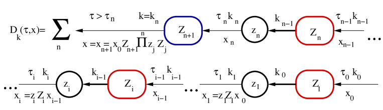
Figure 5: The scheme of kinematics and flavour indices in the hierarchical Markovian.

The iterative solution of the DGLAP equation reorganized in the hierarchical form reads as follows:

$$\begin{split}D_{k}&(\tau,x)=\int dZ\;dx_{0}\;e^{-(\tau-\tau_{0})R_{k}^{\prime}}d_{k}(\tau,Z|\tau_{0})\;D_{k}(\tau_{0},x_{0})\delta_{x=Zx_{0}}+\\ &+\sum_{n=1}^{\infty}\;\sum_{{k_{n-1}\dots,k_{1},k_{0}}\atop{k_{j}\neq k_{j-1},j=1,\dots,n}}\bigg{[}\prod_{j=1}^{n}\int\limits_{\tau_{0}}^{\tau}d\tau_{j}\;\theta_{\tau_{j}>\tau_{j-1}}\bigg{]}\;\int\limits_{0}^{1}dZ_{n+1}\;\bigg{[}\prod_{i=1}^{n}\int\limits_{0}^{1}dz_{i}\;\int\limits_{0}^{1}dZ_{i}\bigg{]}\;\int\limits_{0}^{1}dx_{0}\;\\ &~{}~{}~{}~{}~{}~{}~{}~{}~{}~{}~{}~{}~{}~{}~{}~{}~{}~{}\times e^{-(\tau-\tau_{n})R_{k}^{\prime}}\;\;d_{k}(\tau,Z_{n+1}|\tau_{n})\;\\ &~{}~{}~{}~{}~{}~{}~{}~{}~{}~{}~{}~{}~{}~{}~{}~{}~{}~{}\times\bigg{[}\prod_{i=1}^{n}\mathcal{P}_{k_{i}k_{i-1}}^{\Theta}(z_{i})\;e^{-(\tau_{i}-\tau_{i-1})R_{k_{i-1}}^{\prime}}\;d_{k_{i-1}}(\tau_{i},Z_{i}|\tau_{i-1})\bigg{]}\;\\ &~{}~{}~{}~{}~{}~{}~{}~{}~{}~{}~{}~{}~{}~{}~{}~{}~{}~{}\times D_{k_{0}}(\tau_{0},x_{0})\delta\bigg{(}x-x_{0}\prod_{i=1}^{n}z_{i}\prod_{i=1}^{n+1}Z_{i}\bigg{)},\\ &d_{k}(\tau,Z|\tau_{0})=Z^{-1}e^{-(\tau-\tau_{0})R_{kk}}\bigg{\{}\delta_{Z=1}+\sum_{n=1}^{\infty}\prod_{i=1}^{n}\int\limits_{\tau_{0}}^{\tau}d\tau_{i}\;\theta_{\tau_{i}>\tau_{i-1}}\int\limits_{0}^{1}dz_{i}\;z_{i}\mathcal{P}_{kk}^{\Theta}(z_{i})\delta_{Z=\prod_{i=1}^{n}z_{i}}\bigg{\}},\end{split}$$ (28)

where we denote $k\equiv k_{n}$ and the virtual form factors are defined as follows:

$$\begin{split}&R_{k}\equiv\mathcal{P}_{kk}^{\delta}(\varepsilon)=\sum_{j}\int\limits_{0}^{1}dz\;z\mathcal{P}^{\Theta}_{jk}(z),\qquad\Phi_{k}(\tau,\tau_{0})=(\tau-\tau_{0})R_{k},\\ &R_{jk}=\int\limits_{0}^{1}dz\;z\mathcal{P}^{\Theta}_{jk}(z),\quad R_{k}^{\prime}=\sum_{j\neq k}R_{jk}=R_{k}-R_{kk}.\end{split}$$ (29)

The $d_{k}$-function obeys the normalization condition $\int_{0}^{1}dZ\;Zd_{k}(\tau,Z|\tau_{0})\equiv 1$. It is easy to check that $d_{k}$ is related to the pure bremsstrahlug distribution $\mathcal{D}_{kk}$ worked out in section 3, eq. (11), in the following way:

$$\begin{split}&\mathcal{D}_{kk}(\tau,\tau_{0};Z)=e^{-(\tau-\tau_{0})R^{\prime}_{k}}d_{k}(\tau,Z|\tau_{0}),\\ &R_{k}=b_{k}\ln(1/\varepsilon)-a_{k}.\end{split}$$ (30)

As is also schematically shown in fig. 5, the integrand of eq. (28) consists of a product of the superlevel transition probabilities, each of them consisting of the flavour-changing kernel and the pure bremsstrahlung function. The whole emission chain is terminated with yet another bremsstrahlung function.

Let us add the following interesting side remark: We could interpret the above formula as the Markovian process, each step being an entire (pure bremsstrahlung) Markovian process of its own. Of course, it would be possible to implement such a hierarchical two-level Markovian scenario as the MC simulation of the unconstrained QCD evolution; however, in such a case, contrary to the CMC case, there is no convincing reason to invest an extra effort to implement in practice such a solution.

4.3 The CMC solution type I

Exploiting the two-level hierarchical solution of eq. (28), we shall work out in the following the CMC solution of type I, concentrating on the flavour-changing superlevel, because the pure bremsstrahlung level is the same as described in section 3, except that it is repeated here not once but many times in a single evolution process. As a first step, let us write eq. (28) once again, in a more compact form, eliminating $\int dx_{0}$ at the expense of the $\delta$-function:

$$\begin{split}&D_{k}(\tau,x)=\int dZ\;\mathcal{D}_{kk}(\tau,\tau_{0};Z)\;\frac{\bar{x}_{0}}{x}D_{k}(\tau_{0},\bar{x}_{0})\;\theta_{x<Z}+\\ &~{}~{}~{}+\sum_{n=1}^{\infty}\;\sum_{{k_{n-1}\dots,k_{1},k_{0}}\atop{k_{j}\neq k_{j-1},j=1,\dots,n}}\bigg{[}\prod_{j=1}^{n}\int\limits_{\tau_{0}}^{\tau}d\tau_{j}\;\theta_{\tau_{j}>\tau_{j-1}}\bigg{]}\;\int\limits_{0}^{1}dZ_{n+1}\;\mathcal{D}_{kk}(\tau,\tau_{n};Z_{n+1})\;\\ &~{}~{}~{}~{}~{}~{}\times\bigg{[}\prod_{i=1}^{n}\int\limits_{0}^{1}dz_{i}\;\mathcal{P}_{k_{i}k_{i-1}}^{\Theta}(z_{i})\;\int\limits_{0}^{1}dZ_{i}\;\mathcal{D}_{k_{i-1}k_{i-1}}(\tau_{i},\tau_{i-1};Z_{i})\bigg{]}\;\\ &~{}~{}~{}~{}~{}~{}\times\frac{\bar{x}_{0}}{x}D_{k_{0}}(\tau_{0},\bar{x}_{0})\;\theta_{x<Z_{n+1}\prod_{i=1}^{n}z_{i}Z_{i}},\\ &\bar{x}_{0}\equiv x\bigg{(}Z_{n+1}\prod_{i=1}^{n}z_{i}Z_{i}\bigg{)}^{-1}.\end{split}$$ (31)

Next, we work out the explicit kinematic limits in terms of $x$-variables defined as follows:

$$x_{i}\equiv\bigg{(}\prod_{j=1}^{i}z_{j}Z_{j}\bigg{)}\bar{x}_{0}=x\bigg{(}Z_{n+1}\prod_{j=i+1}^{n}z_{j}Z_{j}\bigg{)}^{-1},\;i=0,1,2,..,n,\quad x_{n+1}\equiv x,\quad z_{n+1}\equiv 1.$$ (32)

In this way, we obtain

$$\begin{split}&D_{k}(\tau,x)=x^{-1}\int_{x}^{1}dZ_{1}\;\mathcal{D}_{kk}(\tau,\tau_{0};Z_{1})\;\bar{x}_{0}D_{k}(\tau_{0},\bar{x}_{0})+\\ &~{}~{}~{}+x^{-1}\sum_{n=1}^{\infty}\;\sum_{{k_{n-1}\dots,k_{1},k_{0}}\atop{k_{j}\neq k_{j-1},j=1,\dots,n}}\bigg{[}\prod_{j=1}^{n}\int\limits_{\tau_{0}}^{\tau}d\tau_{j}\;\theta_{\tau_{j}>\tau_{j-1}}\bigg{]}\;\int\limits_{x}^{1}dZ_{n+1}\;\mathcal{D}_{kk}(\tau,\tau_{n};Z_{n+1})\;\\ &~{}~{}~{}~{}~{}~{}\times\bigg{[}\prod_{i=1}^{n}\int\limits_{x_{i}}^{1}dz_{i}\;\mathcal{P}_{k_{i}k_{i-1}}^{\Theta}(z_{i})\;\int\limits_{x_{i}/z_{i}}^{1}dZ_{i}\;\mathcal{D}_{k_{i-1}k_{i-1}}(\tau_{i},\tau_{i-1};Z_{i})\bigg{]}\;\bar{x}_{0}D_{k_{0}}(\tau_{0},\bar{x}_{0}).\;\end{split}$$ (33)

The functions $\mathcal{D}_{k_{i-1}k_{i-1}}(\tau_{i},\tau_{i-1};Z_{i})$ are the multidimensional integrals of their own, described in section 3, which in the Monte Carlo are implemented as a separate module providing pure bremsstrahlung subevents with the weight $w^{\#}_{k_{i-1}}$. In the first stage of the MC, neglecting $w=\prod_{i}w^{\#}_{k_{i-1}}$, i.e. replacing $\mathcal{D}_{kk}$ by $\mathcal{D}^{\prime}_{kk}$ of eq. (26), we have to generate $3n+1$ continuous variables explicitly present in eq. (33) according to the integrand

$$\begin{split}&D_{k}(\tau,x)=x^{-1}\int\limits_{0}^{(1-x)^{b_{k}(\tau-\tau_{0})}}dU_{1}\;Z(U_{1})^{\omega_{k}-2}e^{a_{k}(\tau-\tau_{0})}\;\bar{x}_{0}D_{k}(\tau_{0},\bar{x}_{0})+\\ &~{}+x^{-1}\sum_{n=1}^{\infty}\;\sum_{{k_{n-1}\dots,k_{1},k_{0}}\atop{k_{j}\neq k_{j-1},j=1,\dots,n}}\bigg{[}\prod_{j=1}^{n}\int\limits_{\tau_{0}}^{\tau}d\tau_{j}\;\theta_{\tau_{j}>\tau_{j-1}}\bigg{]}\;\int\limits_{0}^{(1-x)^{b_{k}(\tau-\tau_{n})}}dU_{n+1}\;Z(U_{n+1})^{\omega_{k}-2}e^{a_{k}(\tau-\tau_{n})}\;\\ &~{}~{}~{}~{}~{}~{}~{}\times\bigg{[}\prod_{i=1}^{n}\int\limits_{x_{i}}^{1}dz_{i}\;\mathcal{P}_{k_{i}k_{i-1}}^{\Theta}(z_{i})\;\int\limits_{0}^{(1-x_{i}/z_{i})^{b_{k_{i-1}}(\tau_{i}-\tau_{i-1})}}dU_{i}\;Z(U_{i})^{\omega_{k_{i-1}}-2}e^{a_{k_{i-1}}(\tau_{i}-\tau_{i-1})}\bigg{]}\;\\ &~{}~{}~{}~{}~{}~{}~{}\times\bar{x}_{0}D_{k_{0}}(\tau_{0},\bar{x}_{0}),\end{split}$$ (34)

where $U_{i}=\exp(\mathcal{R}(Z_{i}))$ and

$$\bar{x}_{0}\equiv x\bigg{(}Z(U_{n+1})\prod_{i=1}^{n}z_{i}Z(U_{i})\bigg{)}^{-1}.$$ (35)

The first term ($n=0$) in the above sum is identical to the one discussed in section 3. The second term for $n=1$ is the new and non-trivial one, representing one $q\to G$ or $G\to q$ transition accompanied by the two segments of the pure bremsstrahlung. It reads as follows:

$$\begin{split}&D_{k}(\tau,x)|_{n=1}=x^{-1}\sum_{{k_{0}}\atop{k\neq k_{0}}}\int\limits_{\tau_{0}}^{\tau}d\tau_{1}\;\int\limits_{0}^{(1-x)^{b_{k}(\tau-\tau_{1})}}dU_{2}\;Z(U_{2})^{\omega_{k}-2}e^{a_{k}(\tau-\tau_{1})}\;\\ &~{}~{}~{}\times\int\limits_{x_{1}}^{1}dz_{1}\;\mathcal{P}_{kk_{0}}^{\Theta}(z_{1})\;\int\limits_{0}^{(1-x_{1}/z_{1})^{b_{k_{0}}(\tau_{1}-\tau_{0})}}dU_{1}\;Z(U_{1})^{\omega_{k_{0}}-2}e^{a_{k_{0}}(\tau_{1}-\tau_{0})}\;\;\bar{x}_{0}D_{k_{0}}(\tau_{0},\bar{x}_{0}),\end{split}$$ (36)

where $x_{1}\equiv x/Z_{2}$, $\bar{x}_{0}\equiv x/(Z_{2}Z_{1}z_{1})$ and $k_{1}\equiv k$.

In addition to continuous variables, we have to solve the problem of generating efficiently all discrete variables $k_{i},i=0,1,\dots,n-1$. For gluon and $2n_{f}$ quarks and antiquarks in the contribution with $n$ flavour transitions, we have in eqs. (31)–(34) up to $(2n_{f}+1)^{n}$ terms. This might be a serious problem in the case of implementing all these component integrals one by one in the general-purpose MC tool such as Foam, taking for example $n\leq n_{\max}=4$. Luckily, thanks to symmetries valid in the LL approximation, we are able to get this problem under control, at least for massless identical quarks. This methodology is not the same as the traditional splitting of parton distributions into singlet and non-singlet parts, although it exploits the same properties of the kernels.

The essence of the solution of the above problem can be demonstrated in a transparent way for just one type of quark and antiquark. The extension to the case of $n_{f}$ identical massless quarks is not difficult and will be done later on. Let us analyse the flavour sum $\sum_{k_{n-1}k_{n-2}\dots k_{1},k_{0}}$, with the condition $k_{i}\neq k_{i-1},i=1,2,\dots,n$, in eq. (34). We split the parton distribution of eq. (34) into components with a well defined number of flavour transitions $D(x)=\sum_{n=0}^{n_{\max}}D^{(n)}$, and we shall discuss the components $D^{(n)}$ one by one. In the above and in the following we omit all bremsstrahlung contributions in $D^{(n)}$, integrations over $z_{i}$, etc., in eq. (34) – we keep track of only the flavour-changing kernels and their indices.

The easiest case is $n$=0, that is the case of the pure bremsstrahlung. Here, the integrand contains just one term proportional to $D_{k}$, modulo the bremsstrahlung part, where $k$ is one of the three possible flavours $k=G,q,\bar{q}$. In the distribution given to Foam this contribution is treated separately and is generated automatically by Foam with the correct probability.

The first non-trivial case is that of $n=1$ and $k=k_{1}=G$. Here, the sum under consideration is $D^{(1)}_{G}=\sum_{k_{0}}\mathcal{P}_{Gk_{0}}D_{k_{0}}$, where $k_{0}\neq G$, hence $k_{0}=q,\bar{q}$. Since $\mathcal{P}_{Gq}=\mathcal{P}_{G\bar{q}}$ we may replace both of them by $\mathcal{P}_{Gq}$ and pull them out of the sum. We obtain $D^{(1)}_{G}=\mathcal{P}_{Gq}\sum_{k_{0}=q,\bar{q}}D_{k_{0}}=\mathcal{P}_{Gq}D_{Q}$, where we have introduced the inclusive (singlet) initial quark distribution $D_{Q}=\sum_{k_{0}=q,\bar{q}}D_{k_{0}}$.

In the similar case $k=k_{1}=q$ for $n=1$, the sum under consideration is $D^{(1)}_{q}=\sum_{k_{0}}\mathcal{P}_{qk_{0}}D_{k_{0}}$. In this case the only possible contribution is for $k_{0}=G$, and the only remaining term is $D^{(1)}_{q}=\mathcal{P}_{qG}D_{G}$. In the case of tagged antiquark, $k_{0}=\bar{q}$, we obtain exactly the same contribution: $D^{(1)}_{\bar{q}}=\mathcal{P}_{qG}D_{G}$.

The general case of the $n>1$ transitions is quite similar to the $n=1$ case. In the case of $k=k_{n}=G$, in the sum

$$D^{(n)}_{G}=\sum_{k_{n-1}k_{n-2}\dots k_{1},k_{0}}\mathcal{P}_{Gk_{n-1}}\dots\mathcal{P}_{k_{1}k_{0}}D_{k_{0}},$$

we may repeat the previous reasoning we followed for $n=1$. In the first step we reduce the summation over the last index $k_{n-1}=q,\bar{q}$ with the help of $\mathcal{P}_{Gq}=\mathcal{P}_{G\bar{q}}$ and $\mathcal{P}_{qG}=\mathcal{P}_{\bar{q}G}$ obtaining:

$$D^{(n)}_{G}=2\mathcal{P}_{Gq}\sum_{k_{n-2}\dots k_{1},k_{0}}\mathcal{P}_{qk_{n-2}}\dots\mathcal{P}_{k_{1}k_{0}}D_{k_{0}}.$$

In the next step we get rid of the sum over $k_{n-2}$

$$D^{(n)}_{G}=2\mathcal{P}_{Gq}\mathcal{P}_{qG}\sum_{k_{n-3}\dots k_{1},k_{0}}\mathcal{P}_{Gk_{n-3}}\dots\mathcal{P}_{k_{1}k_{0}}D_{k_{0}}.$$

We continue with the elimination of the sums one by one, obtaining for odd $n$:

$$D^{(n)}_{G}=2^{(n-1)/2}\;\mathcal{P}_{Gq}\mathcal{P}_{qG}\mathcal{P}_{Gq}\dots\mathcal{P}_{Gq}\;D_{Q},$$

while for even $n$ we obtain:

$$D^{(n)}_{G}=2^{n/2}\;\mathcal{P}_{Gq}\mathcal{P}_{qG}\mathcal{P}_{Gq}\dots\mathcal{P}_{qG}\;D_{G}.$$

As a result of the above reasoning, the whole sum is reduced to just one term for each $n$. (Every $n=0,1,\dots,n_{\max}$ is generated by Foam separately.) It is important to stress that, in the MC, where we are interested in a fully exclusive history of the intermediate states in the emission chain, we may easily undo the summation over equal contributions from quarks and antiquarks, leading to factors $2^{(n-1)/2}$ or $2^{n/2}$, and choose randomly with the probability $1/2$ between $k_{j}=q$ and $k_{j}=\bar{q}$ for every intermediate non-gluon state (every other link in the emission tree).

The case of $k=k_{n}=q$ and $n>1$ can be analysed in an analogous way:

$$D^{(n)}_{q}=\sum_{k_{n-1}k_{n-2}\dots k_{1},k_{0}}\mathcal{P}_{qk_{n-1}}\dots\mathcal{P}_{k_{1}k_{0}}D_{k_{0}}.$$

Due to kernel properties and $k_{n}\neq k_{n-1}$, the condition $D^{(n)}_{q}$ reduces in the first step to:

$$D^{(n)}_{q}=\mathcal{P}_{qG}\sum_{k_{n-2}\dots k_{1},k_{0}}\mathcal{P}_{Gk_{n-2}}\dots\mathcal{P}_{k_{1}k_{0}}D_{k_{0}}.$$

The final result is either

$$D^{(n)}_{q}=2^{(n-1)/2}\;\mathcal{P}_{qG}\mathcal{P}_{Gq}\mathcal{P}_{qG}\dots\mathcal{P}_{Gq}\;D_{Q},\hskip 28.45274pt\hbox{for}~{}n~{}\hbox{odd}$$

or

$$D^{(n)}_{q}=2^{n/2}\;\mathcal{P}_{qG}\mathcal{P}_{Gq}\mathcal{P}_{qG}\dots\mathcal{P}_{qG}\;D_{G},\hskip 28.45274pt\hbox{for}~{}n~{}\hbox{even}.$$

Summarizing, for identical quarks, in the LL approximation, we may effectively get rid of summations over all of the flavour indices! The case of $n_{f}$ identical quarks is quite analogous – the only difference is that we get $(2n_{f})^{(n-1)/2}$ or $(2n_{f})^{n/2}$ weight factors in front of each single final term. When restoring the type of the intermediate quark we choose randomly with equal probability one of the $2n_{f}$ quarks and antiquarks.

The above collective treatment of the intermediate quarks/antiquarks in the process of implementing the distributions of eq. (34) as integrands of Foam is relatively easy for the finite number of flavour transitions ($n=0,1,2,3,4$). As we remember, the only case where we need to explicitly generate an individual quark or antiquark type $k_{0}$ according to $\sim\mathcal{P}_{k_{0}}(x_{0})H_{k_{0}}$, is the case of $n=0$, i.e. pure bremsstrahlung. In all other cases, $n>0$, we may treat quarks and antiquarks at the intermediate stage of the MC generation collectively and randomly choose their individual type (index) later on, with equal probabilities.

In the above explicit algebra, the difference between the traditional split into singlet and non-singlet components $D^{S}=D_{q}+D_{\bar{q}}$ and $D^{NS}=D_{q}-D_{\bar{q}}$ and our alternative split into pure bremsstrahlung component $D_{q}^{(0)}$ or $D_{\bar{q}}^{(0)}$ and the rest $D_{q}^{(n>0)}=D_{\bar{q}}^{(n>0)}$ is manifest. Both techniques exploit, of course, the same symmetry properties of the kernels.

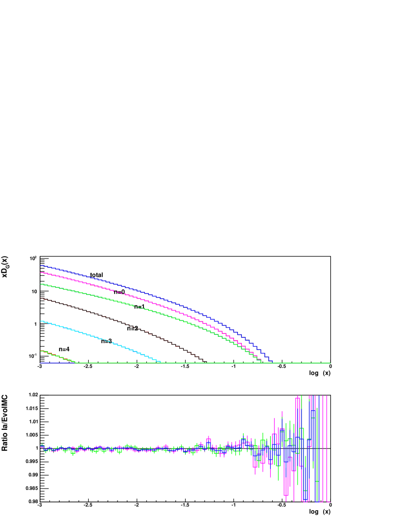
Figure 6: CMC versus Markovian MC for gluons; number of quark–gluon transitions $n=0,1,2,3,4$ and the total. The ratio in the lower plot is for $n=0,1$ and the total (blue).

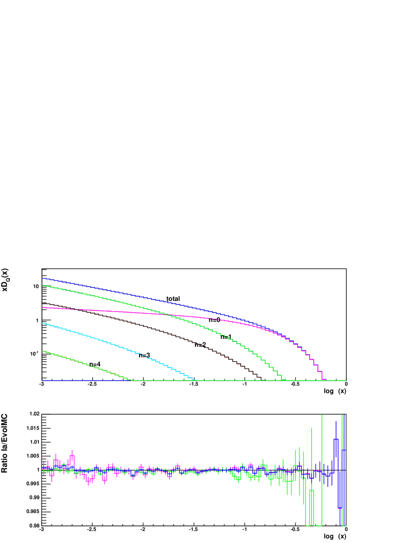
Figure 7: CMC versus Markovian MC for quarks; number of quark-gluon transitions $n=0,1,2,3,4$ and the total. The ratio in the lower plot is for $n=0,1$ and the total (blue).

With all the above algebra at hand, we can formulate our CMC algorithm in the general LL DGLAP case:

• Generate superlevel variables $n$, $k_{i}$, $\tau_{i}$ $Z_{i}$ and $z_{i}$ using the Foam general-purpose MC tool according to eq. (34).

• In the above we limit the number of flavour transitions ($G\to Q$ and $Q\to G$) to $n=0,1,2,3,4$, aiming at a precision of $\sim 0.2\%$.

• For each pure gluon bremsstrahlung segment defined by $Z_{i}$ and $(\tau_{i},\tau_{i-1})$, $i=1,2,...,n+1$, gluon emission variables $(z^{(i)}_{j},\tau^{(i)}_{j}),\;j=1,2,...,n^{(i)}$, are generated using the previously described dedicated CMC.

• Weighted events are generated. They are optionally turned into weight-1 events using the conventional rejection method.

The above algorithm is already implemented in the C++ programming language and tested using Markovian MC EvolMC of refs. [10] and [11]; see next section. In the program construction the central variable is the number of quark–gluon transitions $n$. We do not know the analytical expression for the distribution of this variable. It is one of the variables managed by Foam. In the initialization phase, Foam finds out the distribution of $n$ numerically and then generates $n$ efficiently in the range $0\leq n\leq n_{\max}$. In the CMC program construction the $n_{\max}=0,1$ cases were programmed first and the results were compared with EvolMC. The main programming exercise consist of the careful programming of the integrand distribution for Foam. It was finally done for arbitrary $n_{\max}$. The other part of the programming is related to joining pieces of several pure bremsstrahlung segments into a single long emission chain with an arbitrary number of quark–gluon transitions. Object-oriented programming tools made this task easier.

4.4 The CMC for DGLAP: numerical results

The basic tests of the new CMC algorithm are presented in figs. 6 and 7. As in section 3.1, we examine results of the DGLAP evolution from the energy scale $Q=1$ GeV to $Q=1$ TeV, using as the starting point quark and gluon distributions in proton at $Q=1$ GeV, exactly the same as in ref. [10]. In fig. 6 we show distributions of gluon at $Q=1$ TeV, while in fig. 7 are plotted the results for quark, $Q=q+\bar{q}$, at the same high scale $Q=1$ TeV. In these two figures we compare gluon and quark distributions obtained from the new CMC program and from the Markovian EvolMC of ref. [10]. The main numerical results from both programs, marked as “total” in the upper plot of both figures, are indistinguishable. We therefore plot their ratio in the lower plot of both figures. They agree perfectly well within the statistical error, in the entire range of $x$. For $x<0.1$ the statistical error is below $0.1\%$.

The plots in figs. 6 and 7 contain, however, more tests than that for the total normalization. As already mentioned, in the process of constructing the CMC program we have tested also each “slice” of the gluon and quark distribution for a given number of quark–gluon transitions $n=0,1,2,3,4$, on the way from 1 GeV to 1 TeV. For example, in fig. 6 we show separately the contributions to the gluon distribution from the following evolution histories:
$n=0$: $G\to G$
$n=1$: $Q\to G$ and any number of gluon emissions out of $Q$ and $G$,
$n=2$: $G\to Q\to G$, etc.
$n=3$: $Q\to G\to Q\to G$, etc.
$n=4$: $G\to Q\to G\to Q\to G$, etc. (“Total” is the sum of $n=0,1,2,3,4$.)
They are shown in the upper plot of the figure one by one for the two programs compared, CMC and EvolMC. As before, the results are indistinguishable – this is why we plot their ratios in the lower plot of the figure. The discrepancy is within the statistical error, as in the total contribution. In this plot the comparison of the two programs for the $n=0$ slice is a repetition of the pure bremsstrahlung test from section 3.1, but for much higher statistics.

Analogous slices for the quark distribution:
$n=0$: $Q\to Q$
$n=1$: $G\to Q$ and any number of gluon emissions out of $Q$ and $G$,
$n=2$: $G\to Q\to G\to Q$, etc.
$n=3$: $G\to Q\to G\to Q$, etc.
$n=4$: $Q\to G\to Q\to G\to Q$, etc. (“Total” is the sum of $n=0,1,2,3,4$) are shown in fig. 7. Again the results from the new CMC and Markovian EvolMC agree perfectly well.

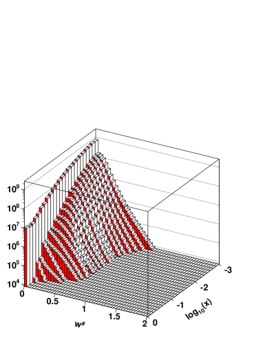
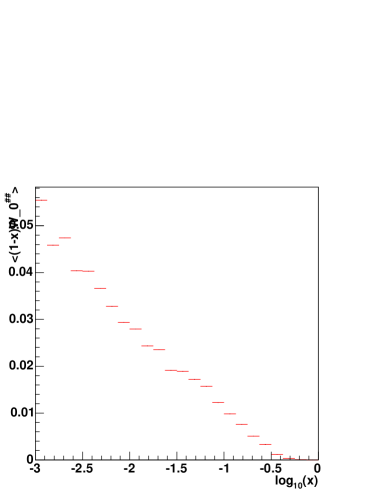
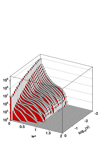
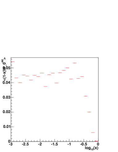
Figure 8: Weight distribution of the new CMC algorithm for gluon (upper plots) and quark (lower plots) as a function of $x$.

In fig. 8 we show the distributions of the MC weight distribution separately for the evolution yielding gluon and quark at $Q=1$ TeV. This is an important technical test of the MC integration/simulation performed with the help of the general-purpose MC tool Foam. As we see, the resulting MC weight is well limited, $w\leq 1$, and the average weight is about 0.08. The efficiency is therefore quite good, substantially better than that for method II.b of ref. [9]. Note that for $n_{\max}=4$ the integrand of Foam is 15-dimensional, but the modelling of this distribution is performed using only 2000 cells. This clearly demonstrates the power and the usefulness of this tool.

5 Conclusions and outlook

In this work we have shown that there exists an efficient constrained Monte Carlo algorithm for the initial-state radiation emission chain in QCD. Its most likely application will be in the construction of a new class of parton shower Monte Carlo event generators for the QCD initial-state radiation.

In this context it is worthwhile to mention that a similar CMC algorithm of class I has been worked out [23] for the HERWIG-type QCD evolution, see ref. [5], i.e. for the $z$-dependent $\alpha_{S}((1-z)Q)$ and $t$-dependent IR cut-off $\epsilon(t)$.

The present CMC solution is restricted to the LL kernels. It will be interesting to extend it to the NLL case. The preparatory step in this direction is already done. In ref. [11] the $\overline{MS}$ NLL kernels are implemented within the Markovian Monte Carlo program. They can be ported to the non-Markovian CMC in the future, if necessary.

Let us stress that the CMC algorithm of this work is not the only one known. For instance an alternative non-Markovian CMC algorithm class II exists; see refs. [24] and [9]. It is defined there for the full DGLAP, although it is implemented/tested for the pure bremsstrahlung only. It has worse MC efficiency than the algorithm presented here and leads to higher dimensionality of the integrand managed by FOAM.

Another possible application of the presented CMC algorithm is the MC modelling of the unintegrated parton distributions, including these based on the CCFM-type evolution, for the purpose of MC simulating $W$ and $Z$ production at LHC. In fact, the unintegrated parton distributions $D_{k}(k_{T},x)$ are already calculated [26] from the one-loop type CCFM model of ref. [27], in the framework of unconstrained Markovian MC.

Acknowledgments
We would like to thank W. Płaczek and T. Sjöstrand for useful discussions. We thank for their warm hospitality the CERN Particle Theory Group where part of this work was done. We thank to ACK Cyfronet AGH Computer Center for granting us access to their PC clusters funded by the European Commission grant: IST-2001-32243 and the Polish State Committee for Scientific Research grants: 620/E-77/SPB/5PR UE/DZ 224/2002-2004 and 112/E-356/SPB/5PR UE/DZ 224/2002-2004

Appendix: QCD LL kernels

We present here a table of the elements in the LL kernels ($T_{f}=n_{f}T_{R}$), $Q=q+\bar{q}$

$IK$	$A^{(0)}_{KK}$	$B^{(0)}_{KK}$	$C^{(0)}_{IK}$	$D^{(0)}_{IK}(z)$	$\hat{D}_{IK}(z)$	$\int dzD^{(0)}_{IK}(z)$
$GG$	$\frac{11}{6}C_{A}-\frac{2}{3}T_{f}$	$2C_{A}$	$2C_{A}$	$2C_{A}(-2+z-z^{2})$	$0$	$-\frac{11}{3}C_{A}$
$QG$	$-$	$-$	$0$	$2T_{f}(z^{2}+(1-z)^{2})$	$2T_{f}$	$\frac{4}{3}T_{f}$
$QQ$	$\frac{3}{2}C_{F}$	$2C_{F}$	$0$	$C_{F}(-1-z)$	$0$	$-\frac{3}{2}C_{F}$
$GQ$	$-$	$-$	$2C_{F}$	$C_{F}(-2+z)$	$0$	$-\frac{3}{2}C_{F}$

$$P_{ik}(z)=\delta(1-z)\delta_{ik}A_{kk}+\frac{1}{(1-z)_{+}}\delta_{ik}B_{kk}+\frac{1}{z}C_{ik}+D_{ik}(z).$$ (37)

Temporary simplifications for the purpose of the MC generation are:

$$\begin{split}&zP^{\Theta}_{GG}(z)\to z\hat{P}^{\Theta}_{GG}(z)=zB_{GG}\theta_{1-z>\varepsilon}\left(\frac{1}{1-z}+\frac{1}{z}\right)=B_{GG}\frac{\theta_{1-z>\varepsilon}}{1-z},\\ &zP^{\Theta}_{qq}(z)\to z\hat{P}^{\Theta}_{qq}(z)=B_{qq}\frac{\theta_{1-z>\varepsilon}}{1-z},\\ &z\mathcal{P}^{\Theta}_{kk}(t,z)\to z\hat{\mathcal{P}}^{\Theta}_{kk}(t,z)=\frac{\alpha_{S}(t)}{\pi}\;z\hat{P}^{\Theta}_{kk}(z)=\frac{2B_{kk}}{\beta_{0}(t-t_{\Lambda})}\;\frac{\theta_{1-z>\varepsilon}}{1-z},\\ &\mathcal{P}^{\delta}_{kk}(t)=\frac{\alpha_{S}(t)}{\pi}\bigg{\{}B_{kk}\ln\frac{1}{\varepsilon}-A_{kk}\bigg{\}}.\end{split}$$ (38)

References

-
[1]
L.N. Lipatov, Sov. J. Nucl. Phys. 20 (1975) 95;
V.N. Gribov and L.N. Lipatov, Sov. J. Nucl. Phys. 15 (1972) 438;
G. Altarelli and G. Parisi, Nucl. Phys. 126 (1977) 298;
Yu. L. Dokshitzer, Sov. Phys. JETP 46 (1977) 64. - [2] R. Ellis, W. Stirling, and B. Webber, QCD and Collider Physics. Cambridge University Press, 1996.
- [3] N. G. van Kampen, Stochastic Processes in Physics and Chemistry. North Holland, 1981.
- [4] T. Sjostrand, Phys. Lett. B157 (1985) 321.
- [5] G. Marchesini and B. R. Webber, Nucl. Phys. B310 (1988) 461.
- [6] T. Sjostrand et al., Comput. Phys. Commun. 135 (2001) 238–259, hep-ph/0010017.
- [7] G. Corcella et al., JHEP 01 (2001) 010, hep-ph/0011363.
-
[8]
M. Ciafaloni, Nucl. Phys. B296 (1988) 49;
S. Catani, F. Fiorani and G. Marchesini, Phys. Lett. B234 339, Nucl. Phys. B336 (1990) 18;
G. Marchesini, Nucl. Phys. B445 (1995) 49. - [9] S. Jadach and M. Skrzypek, Acta Phys. Polon. B36 (2005) 2979–3021, hep-ph/0504205.
- [10] S. Jadach and M. Skrzypek, Acta Phys. Polon. B35 (2004) 745–756, hep-ph/0312355.
- [11] K. Golec-Biernat, S. Jadach, W. Placzek, and M. Skrzypek, Report IFJPAN-V-04-08, hep-ph/0603031.
- [12] S. Frixione and B. R. Webber, JHEP 06 (2002) 029, hep-ph/0204244.
- [13] P. Nason, JHEP 11 (2004) 040, hep-ph/0409146.
- [14] S. Jadach, M. Skrzypek, and Z.Wa̧s, Report IFJPAN-V-04-09.
-
[15]
L. Van Hove, Nucl. Phys. B9 (1969) 331;
W. Kittel, W. Wójcik, L. Van Hove, Comput. Phys. Commun. 1 (1970) 425. - [16] S. Jadach, Comput. Phys. Commun. 9 (1975) 297.
- [17] S. Jadach, MPI-PAE/PTh 6/87, preprint of MPI München, unpublished.
- [18] S. Jadach and B. F. L. Ward, Comput. Phys. Commun. 56 (1990) 351–384.
- [19] S. Jadach, Comput. Phys. Commun. 130 (2000) 244–259, physics/9910004.
- [20] S. Jadach, Comput. Phys. Commun. 152 (2003) 55–100, physics/0203033.
- [21] M. Botje, ZEUS Note 97-066, http://www.nikhef.nl/ h24/qcdcode/.
- [22] K. Golec-Biernat, the Fortran code to be obtained from the author, unpublished.
- [23] S. Jadach and M. Skrzypek, Report CERN-PH-TH/2005-146, IFJPAN-V-05-09, Contribution to the HERA–LHC Workshop, CERN–DESY, 2004–2005, http://www.desy.de/heralhc/, hep-ph/0509178.
- [24] S. Jadach and M. Skrzypek, Nucl. Phys. Proc. Suppl. 135 (2004) 338–341.
- [25] H. Jung and G. P. Salam, Eur. Phys. J. C19 (2001) 351–360, hep-ph/0012143.
- [26] K. Golec-Biernat, S. Jadach, M. Skrzypek, and W. Płaczek, report IFJPAN-V-05-03, in preparation.
- [27] G. Marchesini and B. R. Webber, Nucl. Phys. B349 (1991) 617–634.