Monte Carlo simulation of events with Drell-Yan lepton pairs from antiproton-proton collisions: the fully polarized case

Abstract

In this paper, we extend the study of Drell-Yan processes with antiproton beams already presented in a previous work. We consider the fully polarized $\bar{p}^{\uparrow}p^{\uparrow}\rightarrow\mu^{+}\mu^{-}X$ process, because this is the simplest scenario for extracting the transverse spin distribution of quarks, or transversity, which is the missing piece to complete the knowledge of the nucleon spin structure at leading twist. We perform Monte Carlo simulations for transversely polarized antiproton and proton beams colliding at a center-of-mass energy of interest for the future HESR at GSI. The goal is to possibly establish feasibility conditions for an unambiguous extraction of the transversity from data on double spin asymmetries.

I Introduction

Building the nonperturbative structure of the nucleon bound state in QCD requires, first of all, the knowledge of the leading (spin) structure of the nucleon in terms of quarks and gluons. The transverse spin distribution (in jargon, transversity) constitutes the missing cornerstone that completes such knowledge together with the well known and measured unpolarized and helicity distributions Artru and Mekhfi (1990); Jaffe and Ji (1991); Jaffe (1996); Barone and Ratcliffe (2003).

From the technical point of view, the transversity is not diagonal in the parton helicity basis, hence the jargon of chiral-odd function. But in the transverse spin basis it is diagonal and it can be given the probabilistic interpretation of the mismatch between the numbers of partons with spin parallel or antiparallel to the transverse polarization of the parent hadron. In a nucleon (and, in general, for all hadrons with spin $\textstyle{\frac{1}{2}}$), the gluon has no transversity because of the mismatch in the change of helicity units; hence, the evolution of transversity for quarks decouples from radiative gluons. But it also decouples from charge-even $q\bar{q}$ configurations of the Dirac sea, because it is odd also under charge conjugation transformations. In conclusion, the transversity should behave like a nonsinglet function, describing the distribution of a valence quark spoiled by any radiative contribution Jaffe (1996). The prediction of a weaker evolution of transversity with respect to the helicity distribution is counterintuitive and it represents a basic test of QCD in the nonperturbative domain.

The first moment of transversity is related to the chiral-odd twist-2 tensor operator $\sigma^{\mu\nu}\gamma_{5}$, which is not part of the hadron full angular momentum tensor Jaffe (1996). Therefore, the transversity is not related to some partonic fraction of the nucleon spin, but it opens the door to studies of chiral-odd QCD operators and, more generally, of the role of chiral symmetry breaking in the nucleon structure. In particular, another basic test of QCD should be possible, namely to verify the prediction that the nucleon tensor charge is much larger than its helicity, as it emerges from preliminary lattice studies Aoki et al. (1997).

From the experimental point of view, the transversity is quite an elusive object: being chiral-odd, it needs to be coupled to a chiral-odd partner inside the cross section. As such, it is systematically suppressed in inclusive Deep-Inelastic Scattering (DIS) Jaffe and Ji (1993). The first pioneering work about the strategy for its measurement suggested the production of Drell-Yan lepton pairs from the collision of two transversely polarized proton beams Ralston and Soper (1979). By flipping the spin of one of the two beams, it is possible to build a double spin asymmetry in the azimuthal angle of the final pair, that displays at leading twist the factorized product of the two transversities for the colliding quark-antiquark pair. This is the simplest possible scenario, since no other unknown functions are involved. But, in principle, the transverse spin distribution of an antiquark in a transversely polarized proton cannot be large. Moreover, the combined effect of evolution and of the Soffer inequality seems to constrain the double spin asymmetry to very small values Martin et al. (1998); Barone et al. (1997).

Alternatively, in semi-inclusive reactions the transversity can appear in the leading-twist part of the cross section together with a suitable chiral-odd fragmentation function Mulders and Tangerman (1996). For 1-pion inclusive production, like in $pp^{\uparrow}\rightarrow\pi X$ or $ep^{\uparrow}\rightarrow e^{\prime}\pi X$ reactions, the chiral-odd partner can be identified with the Collins function Collins (1993). However, the situation is not so clear, since other competitive mechanisms (like, e.g., the Sivers effect Sivers (1990)) can produce the same single spin asymmetry when flipping the spin of the transversely polarized target. This happens because one crucial requirement is that the spin asymmetry must keep memory of the transverse momentum of the detected pion with respect to the jet axis, and, consequently, of the intrinsic transverse momentum of the parton. Several nonperturbative mechanisms can be advocated to relate the latter to the transverse polarization (see, among others, the Refs. Gamberg et al. (2003); Bacchetta et al. (2004); Efremov et al. (2003); Anselmino et al. (2005)), ultimately involving the orbital angular motion of partons inside hadrons Brodsky et al. (2002); Belitsky et al. (2003); Burkardt and Hwang (2004).

Rapid developments are emerging in this field. In particular, new azimuthal asymmetries are being deviced to extract the transversity at leading twist while, at the same time, circumventing the problem of an explicit dependence upon the transverse momentum. When the 2-pion inclusive production Collins and Ladinsky (1994) is considered both in hadronic collisions Bacchetta and Radici (2004a) and lepton DIS with a transversely polarized target Bacchetta and Radici (2003); Bacchetta and Radici (2004b), the chiral-odd partner of transversity is represented by the interference fragmentation function $H_{1}^{{<\kern-2.10002pt{\scriptscriptstyle)}}}$ Bianconi et al. (2000), of which a specific momentum enters the leading-twist single spin asymmetry depending only upon the total momentum and invariant mass of the pion pair Radici et al. (2002); Jaffe et al. (1998).

Experimentally, some recent measurements of semi-inclusive reactions with hadronic Bravar (2000) and leptonic Airapetian et al. (2004) beams have been performed using pure transversely polarized proton targets. New experiments are planned in several laboratories (HERMES at DESY, CLAS at TJNAF, COMPASS at CERN, RHIC at BNL). In particular, we mention the new project of an antiproton factory at GSI in the socalled High Energy Storage Ring (HESR). In fact, the option of having collisions of (transversely polarized) proton and antiproton beams should make it possible to study single and double spin asymmetries in Drell-Yan processes PAX Collab. (2004); Lenisa et al. (2004); ASSIA Collab. (2004); Maggiora (2005); Efremov et al. (2004); Anselmino et al. (2004) with the further advantage of involving unsuppressed distributions of valence partons, like the transversely polarized antiquark in a transversely polarized antiproton.

In a previous paper Bianconi and Radici (2004), we have explored the Drell-Yan processes $\bar{p}\,p^{(\uparrow)}\rightarrow\mu^{+}\,\mu^{-}\,X$. For the single-polarized one, in the leading-twist single spin asymmetry the transversity happens convoluted with another chiral-odd function Boer (1999), which is likely to be responsible for the well known (and yet unexplained) violation of the Lam-Tung sum rule, an anomalous azimuthal asymmetry in the corresponding unpolarized cross section Falciano et al. (1986); Guanziroli et al. (1988); Conway et al. (1989). Monte Carlo simulations have been performed for several kinematic configurations of interest for HESR at GSI, in order to estimate the minimum number of events needed to unambiguously extract the above chiral-odd distributions from a combined analysis of the two asymmetries.

In this paper, we will extend that work by considering numerical simulations for the fully polarized Drell-Yan process $\bar{p}^{\uparrow}\,p^{\uparrow}\rightarrow\mu^{+}\,\mu^{-}\,X$, again at several kinematic configurations of interest for the HESR project at GSI. Since this is the simplest possible combination at leading twist involving, moreover, the dominant valence contribution of the transversity, the goal is to possibly establish feasibility conditions for its unambiguous direct extraction from data on double spin asymmetries. Most of the details of the simulation have been presented in Ref. Bianconi and Radici (2004) and they will be briefly reviewed in Sec. II, together with a description of the kinematics. Results are discussed in Sec. III and some final conclusions are drawn in Sec. IV.

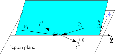
Figure 1: The Collins-Soper frame.

II Theoretical framework and numerical simulations

In a Drell-Yan process, a lepton with momentum $k_{1}$ and an antilepton with momentum $k_{2}$ (with $k_{1(2)}^{2}\sim 0$) are produced from the collision of two hadrons with momentum $P_{1}$, mass $M_{1}$, spin $S_{1}$, and $P_{2},M_{2},S_{2}$, respectively (with $P_{1(2)}^{2}=M_{1(2)}^{2},\;S_{1(2)}^{2}=-1,\;P_{1(2)}\cdot S_{1(2)}=0$). The center-of-mass (cm) square energy available is $s=(P_{1}+P_{2})^{2}$ and the invariant mass of the final lepton pair is given by the time-like momentum transfer $q^{2}\equiv M^{2}=(k_{1}+k_{2})^{2}$. In the kinematical regime where $M^{2},s\rightarrow\infty$, while keeping the ratio $0\leq\tau=M^{2}/s\leq 1$ limited, the lepton pair can be assumed to be produced from the elementary annihilation of a parton and an antiparton with momenta $p_{1}$ and $p_{2}$, respectively. If $P_{1}^{+}$ and $P_{2}^{-}$ are the dominant light-cone components of hadron momenta in this regime, then the partons are approximately collinear with the parent hadrons and carry the light-cone momentum fractions $0\leq x_{1}=p_{1}^{+}/P_{1}^{+},\;x_{2}=p_{2}^{-}/P_{2}^{-}\leq 1$, with $q^{+}=p_{1}^{+},\;q^{-}=p_{2}^{-}$ by momentum conservation Boer (1999). It is usually convenient to study the problem in the socalled Collins-Soper frame Collins and Soper (1977) (see Fig. 1), where

$$\hat{t} = \frac{q}{\sqrt{q^{2}}}$$

$$\hat{z} = \frac{x_{1}P_{1}}{\sqrt{q^{2}}}-\frac{x_{2}P_{2}}{\sqrt{q^{2}}}$$

$$\hat{h} = \frac{q_{{}_{T}}}{|{\bf q}_{{}_{T}}|}\;,$$ (1)

and ${\bf q}_{{}_{T}}$ is the transverse momentum of the final lepton pair detected in the solid angle $(\theta,\phi)$. Azimuthal angles are measured in a plane perpendicular to $\hat{z},\hat{t}$, and containing $\hat{h}$.

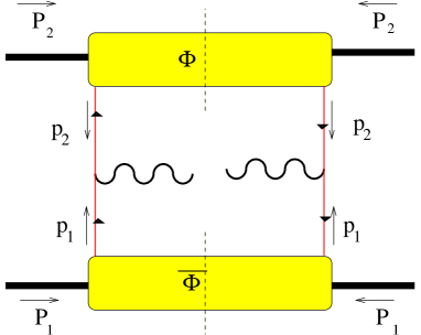
Figure 2: The leading-twist contribution to the Drell-Yan process.

II.1 Double spin asymmetry

If the invariant mass $M$ is not close to the values of known vector resonances, under the above mentioned conditions for factorization the elementary annihilation can be assumed to proceed through a virtual photon converting into the final lepton pair. Then, the leading-order contribution is represented in Fig. 2 Ralston and Soper (1979). The hadronic tensor is given by

$$W^{\mu\nu}=\frac{1}{3}\int dp_{1}^{-}dp_{2}^{+}\,\mbox{Tr}\left[\bar{\Phi}(p_{1};P_{1},S_{1})\,\gamma^{\mu}\,\Phi(p_{2};P_{2},S_{2})\,\gamma^{\nu}\right]\Bigg{|}_{p_{1}^{+}=x_{1}P_{1}^{+},\,p_{2}^{-}=x_{2}P_{2}^{-}}\,+\,\left(\begin{array}[]{ccc}q&\leftrightarrow&-q\\ \mu&\leftrightarrow&\nu\end{array}\right)\;,$$ (2)

where the nonlocal correlators for the annihilating antiparton (labeled ”1”) and parton (labeled ”2”) are defined as

$$\bar{\Phi}(p_{1};P_{1},S_{1}) = \int\frac{d^{4}z}{(2\pi)^{4}}\,e^{-ip_{1}\cdot z}\,\langle P_{1}S_{1}|\psi(z)\,\bar{\psi}(0)|P_{1},S_{1}\rangle\;,$$

$$\Phi(p_{2};P_{2},S_{2}) = \int\frac{d^{4}z}{(2\pi)^{4}}\,e^{ip_{2}\cdot z}\,\langle P_{2},S_{2}|\bar{\psi}(0)\,\psi(z)|P_{2},S_{2}\rangle\;.$$ (3)

They correspond to the blobs in Fig. 2 and contain all the soft mechanisms building up the distribution of the two annihilating partons inside the corresponding hadrons.

Inserting into Eq. (3) the leading-twist parametrization for $\Phi$ and $\bar{\Phi}$ in terms of the (un)polarized partonic distribution functions Boer and Mulders (1998), the Drell-Yan differential cross section for transversely polarized hadrons, after integrating upon $d{\bf q}_{{}_{T}}$, becomes Tangerman and Mulders (1995)

$$\frac{d\sigma^{\uparrow\uparrow}}{dx_{1}\,dx_{2}\,d\Omega} = \frac{\alpha^{2}}{12q^{2}}\,\Bigg{[}(1+\cos^{2}\theta)\,\sum_{f}\,e_{f}^{2}\,\bar{f}^{f}_{1}(x_{1})\,f_{1}^{f}(x_{2})$$ (4)

$$\;+\sin^{2}\theta\,\cos 2\phi\,\frac{\tilde{\nu}(x_{1},x_{2})}{2}$$

$$\;+|{\bf S}_{{}_{T1}}|\,|{\bf S}_{{}_{T2}}|\,\sin^{2}\theta\,\cos(2\phi-\phi_{{}_{S_{1}}}-\phi_{{}_{S_{2}}})\,\sum_{f}\,e_{f}^{2}\,\bar{h}^{f}_{1}(x_{1})\,h_{1}^{f}(x_{2})$$

$$\quad+(1\leftrightarrow 2)\Bigg{]}\;,$$

where $\alpha$ is the fine structure constant, $d\Omega=\sin\theta d\theta d\phi$, $e_{f}$ is the charge of the parton with flavor $f$, and $\phi_{{}_{S_{i}}}$ is the azimuthal angle of the transverse spin of hadron $i$ as it is measured with respect to the lepton plane in a plane perpendicular to $\hat{z}$ and $\hat{t}$ (see Fig. 1). The function $f^{f}_{1}(x)$ is the usual distribution of unpolarized partons with flavor $f$, carrying a fraction $x$ of the unpolarized parent hadron; $h_{1}^{f}(x)$ is the transversity for the same flavor and momentum fraction (analogously for the antiparton distributions). The function $\tilde{\nu}$ contains the contribution of the parton distribution $h_{1}^{\perp}$ Boer (1999), which describes the influence of the (anti)parton transverse polarization on its momentum distribution inside an unpolarized parent hadron: it is believed to be responsible for the observed anomalous azimuthal asymmetry in the unpolarized Drell-Yan cross section, the socalled violation of the Lam-Tung sum rule Falciano et al. (1986); Guanziroli et al. (1988); Conway et al. (1989), which no QCD calculation is presently able to justify in a consistent way Brandenburg et al. (1993, 1994); Eskola et al. (1994).

The double spin asymmetry is defined as

$$A_{{}_{TT}} = \frac{d\sigma^{\uparrow\uparrow}-d\sigma^{\uparrow\downarrow}}{d\sigma^{\uparrow\uparrow}+d\sigma^{\uparrow\downarrow}}$$ (5)

$$= |{\bf S}_{{}_{T1}}|\,|{\bf S}_{{}_{T2}}|\,\frac{\sin^{2}\theta}{1+\cos^{2}\theta}\,\cos(2\phi-\phi_{{}_{S_{1}}}-\phi_{{}_{S_{2}}})\,\frac{\sum_{f}\,e_{f}^{2}\,\bar{h}^{f}_{1}(x_{1})\,h_{1}^{f}(x_{2})+(1\leftrightarrow 2)}{\sum_{f}\,e_{f}^{2}\,\bar{f}^{f}_{1}(x_{1})\,f_{1}^{f}(x_{2})+(1\leftrightarrow 2)}\;.$$

In the next Section, we describe the details for numerically simulating $A_{{}_{TT}}$ using the cross section (4).

II.2 The Monte Carlo simulation

In this Section, we discuss numerical simulations of the double spin asymmetry $A_{{}_{TT}}$ of Eq. (5) for the $\bar{p}^{\uparrow}p^{\uparrow}\rightarrow\mu^{+}\mu^{-}X$ process. Our goal is to explore if it is possible to establish precise conditions in order to determine the feasibility of an unambiguous extraction of the transversity from data. Most of the technical details of the present simulation are mutuated from a previous work, where we performed a similar analysis for the unpolarized and single-polarized Drell-Yan process. Therefore, we will heavily refer to Ref. Bianconi and Radici (2004) and references therein, in the following.

As for the kinematics, several options have been considered in Ref. Bianconi and Radici (2004). Since the cross section decreases for increasing $\tau$, events statistically tend to accumulate in the phase space part corresponding to small $\tau$, where $x_{p}(x_{\bar{p}})$ fall into the range 0.1-0.3 dominated by the valence contributions. In fact, the phase space for large $\tau=x_{p}x_{\bar{p}}$ is scarcely populated because the virtual photon introduces a $1/M^{2}\propto 1/\tau$ factor and the parton distributions become negligible for $x_{p}(x_{\bar{p}})\rightarrow 1$. Since the spectrum of very low invariant masses contains many vector resonances, where the elementary annihilation cannot be simply described by a diagram like the one in Fig. 2, it seems more convenient to reach such low values of $\tau$ by adequately increasing the cm square energy $s$ Bianconi and Radici (2004). Moreover, in this case the elementary annihilation should not be significantly affected by higher-order corrections like subleading twists, and the leading-twist theoretical framework depicted in Sec. II.1 should be reliable. Hence, for the HESR at GSI the most convenient setup seems to be the option where antiprotons with energy $E_{\bar{p}}$ collide against protons with energy $E_{p}$. Nevertheless, as in Ref. Bianconi and Radici (2004) we will explore also the option where the antiproton beam with the same energy hits a fixed proton target.

As for the collider mode, neglecting hadron masses we have

$$s\ =\ (P_{p}+P_{\bar{p}})^{2}\ \approx\ 4\,E_{p}\,E_{\bar{p}}\;,$$ (6)

because for the two colliding beams ${\bf\hat{P}}_{p}=-{\bf\hat{P}}_{\bar{p}}$. As in Ref. Bianconi and Radici (2004), we will select the kinematics where antiprotons have energy $E_{\bar{p}}=15$ GeV and protons $E_{p}=3.3$ GeV, such that $s\sim 200$ GeV². If $M$ is constrained in the ”safe” range 4-9 GeV between the $\bar{c}c$ threshold and the first resonance of the $\Upsilon$ family, then $\tau$ falls into the statistically significant range 0.08-0.4 where the parton distribution functions are dominated by the valence contribution. At the same cm energy, we will consider also the range $1.5\leq M\leq 2.5$ GeV between the $\phi$ and $J/\psi$ resonances, which corresponds to the even lower range $0.01\lesssim\tau\lesssim 0.03$.

For the fixed target mode, which at present is the selected setup by the PANDA collaboration at HESR at GSI PANDA Collab. (2004), we have approximately

$$s=(P_{p}+P_{\bar{p}})^{2}\approx 2\,M_{p}\,E_{\bar{p}}\;,$$ (7)

such that for the considered $E_{\bar{p}}=15$ GeV it results $s\approx 30$ GeV². For this case, we will restrict the invariant mass to the range $1.5\leq M\leq 2.5$ GeV, corresponding to $0.07\leq\tau\leq 0.2$. In fact, for $M>4$ GeV most events are characterized by large partonic fractional momenta, where the quark-antiquark fusion model cannot explain the dimuon production.

The Monte Carlo events have been generated by the following cross section Bianconi and Radici (2004):

$$\frac{d\sigma}{d\Omega dx_{{}_{F}}d\tau d{\bf q}_{{}_{T}}}=K\,\frac{1}{s}\,A({\bf q}_{{}_{T}},x_{{}_{F}},M)\,F(x_{{}_{F}},\tau)\,\sum_{i=1}^{4}\,c_{i}({\bf q}_{{}_{T}},x_{{}_{F}},\tau)\,S_{i}(\theta,\phi,\phi_{{}_{S_{p}}},\phi_{{}_{S_{\bar{p}}}})\;,$$ (8)

or, equivalently,

$$\frac{d\sigma}{d\Omega dx_{\bar{p}}dx_{p}d{\bf q}_{{}_{T}}}=K\,\frac{1}{s}\,(x_{\bar{p}}+x_{p})\,A({\bf q}_{{}_{T}},x_{\bar{p}}-x_{p},M)\,F^{\prime}(x_{\bar{p}},x_{p})\,\sum_{i=1}^{4}\,c^{\prime}_{i}({\bf q}_{{}_{T}},x_{\bar{p}},x_{p})\,S_{i}(\theta,\phi,\phi_{{}_{S_{p}}},\phi_{{}_{S_{\bar{p}}}})\;,$$ (9)

where the invariant $x_{{}_{F}}=x_{\bar{p}}-x_{p}$ is the fraction of the available total longitudinal momentum carried by the two annihilating partons in the collision cm frame. As it has been stressed in Ref. Bianconi and Radici (2004), the range of values for $x_{{}_{F}}$ depends on the energy. For the considered case of $E_{\bar{p}}=15$ GeV, it results $-0.9\leq x_{{}_{F}}\leq 0.9$, where positive values correspond to small $\theta$ angles in the Collins-Soper frame (see Fig. 1), and viceversa. Equations (8) and (9) imply the approximation of a factorized transverse-momentum dependence, which has been achieved by assuming the following phenomenological parametrization

$$A(q_{{}_{T}},x_{{}_{F}},M)=\frac{5\,\displaystyle{\frac{a}{b}\,\left[\frac{q_{{}_{T}}}{b}\right]^{a-1}}}{\left[1+\left(\displaystyle{\frac{q_{{}_{T}}}{b}}\right)^{a}\right]^{6}}\;,$$ (10)

where $a(x_{{}_{F}},M),\,b(x_{{}_{F}},M),$ are parametric polynomials given in Appendix A of Ref. Conway et al. (1989) and $q_{{}_{T}}=|{\bf q}_{{}_{T}}|$. Actually, the Drell-Yan events studied in Ref. Conway et al. (1989) were produced by $\pi-p$ collisions; however, the same analysis, repeated for $\bar{p}-p$ collisions Anassontzis et al. (1988), gives a similar distribution for $q_{{}_{T}}$ not very close to 0 and not much larger than 3 GeV/c. In addition, the above $q_{{}_{T}}$ distribution was fitted for $M>4$ GeV and is singular near $M=1.5$ GeV Conway et al. (1989); for $M<4$ GeV we have assumed the same form with the mass parameter in the coefficients $a$ and $b$ fixed to the value $M=4$ GeV.

In order to simulate Eq. (4), the events produced by Eqs. (8) or (9) have been integrated in $d{\bf q}_{{}_{T}}$. However, apart from theoretical problems related to unwanted soft mechanisms, it is anyway not possible to collect events with very small $q_{{}_{T}}$ because of the collider configuration. Hence, events have been selected with $q_{{}_{T}}>1$ GeV/$c$. In our previous work Bianconi and Radici (2004), the searched asymmetry was emphasized by this threshold. Here, no such enhancement can be present, of course, because of the further integration. But the unavoidable dependence in $q_{{}_{T}}$, introduced by the lower cutoff, reflects in a drastic variation of the size of the sample. A precise answer depends on the experimental setup, but for $q_{{}_{T}}>1$ GeV/$c$ approximately 50% of the initial sample is excluded, while for $q_{{}_{T}}>0.5$ GeV/$c$ this fraction of events is reduced to 20%.

The experimental observation that Drell-Yan pairs are usually distributed with $q_{{}_{T}}>1$ GeV/$c$ Conway et al. (1989), suggests that soft mechanisms are suppressed, because confinement induces much smaller quark intrinsic transverse momenta, but for the same reason it also indicates sizeable QCD corrections to the simple parton model. QCD corrections in the Leading-Log Approximation (LLA) Altarelli et al. (1979) would imply a logarithmic dependence on the scale $M^{2}$ inside the various parameters entering the parton distributions Buras and Gaemers (1978) contained in Eqs. (8) and (9), such that it would determine their DGLAP evolution. However, it must be stressed that the key scale is $M$, and its range here explored is the same of Refs. Conway et al. (1989); Anassontzis et al. (1988), where the functions $F$ and $c_{i}$ in Eq. (8) [or $F^{\prime}$ and $c^{\prime}_{i}$ in Eq. (9)] are assumed to be independent of $M$. In particular, $F^{\prime}$ is given by

$$F^{\prime}(x_{\bar{p}},x_{p})=\frac{\alpha^{2}}{12Q^{2}}\,\sum_{f}\,e_{f}^{2}\,\bar{f}_{1}^{f}(x_{\bar{p}})\,f_{1}^{f}(x_{p})+(\bar{p}\leftrightarrow p)\;,$$ (11)

i.e. it is the azimuthally symmetric unpolarized part of Eq. (4) which has been factorized out. The unpolarized distribution $f_{1}^{f}(x)$ for various flavors $f=u,d,s$, is parametrized as in Ref. Anassontzis et al. (1988). QCD corrections in the Next-to-Leading-Log Approximation (NLLA) Altarelli et al. (1979) are responsible for the well known $K$ factor, which is roughly independent of $x_{{}_{F}}$ and $M^{2}$ but it grows like $\sqrt{\tau}$ Conway et al. (1989). In accordance with Ref. Bianconi and Radici (2004), for the range of interest $0.08\lesssim\tau\lesssim 0.4$ we assume as the best compromise the constant value $K=2.5$. But we observe that in an azimuthal asymmetry the corrections to the cross sections in the numerator and in the denominator should compensate each other; indeed, the smooth dependence of the spin asymmetry on NLLA corrections has been confirmed for fully polarized Drell-Yan processes at high cm square energies Martin et al. (1998).

The whole solid angle $(\theta,\phi)$ of the final muon pair in the Collins-Soper frame is randomly distributed in each variable. From Eq. (4), the explicit form of the $q_{{}_{T}}$-integrated angular distribution is

$$\sum_{i=1}^{4}\,c^{\prime}_{i}(x_{\bar{p}},x_{p})\,S_{i}(\theta,\phi,\phi_{{}_{S_{p}}},\phi_{{}_{S_{\bar{p}}}}) = 1+\cos^{2}\theta$$ (12)

$$+\frac{\nu(x_{\bar{p}},x_{p})}{2}\,\sin^{2}\theta\,\cos 2\phi$$

$$+|{\bf S}_{{}_{Tp}}|\,|{\bf S}_{{}_{T\bar{p}}}|\,c_{4}(x_{\bar{p}},x_{p})\,\sin^{2}\theta\,\cos(2\phi-\phi_{{}_{S_{p}}}-\phi_{{}_{S_{\bar{p}}}})\;.$$

Recalling that the azimuthally symmetric unpolarized part $F^{\prime}(x_{\bar{p}},x_{p})$ of the cross section has been factorized out, the functions $\nu$ and $c_{4}$ turn out to be

$$\nu(x_{\bar{p}},x_{p}) = \frac{\tilde{\nu}(x_{\bar{p}},x_{p})}{\sum_{f}\,e_{f}^{2}\,\bar{f}_{1}^{f}(x_{\bar{p}})\,f_{1}^{f}(x_{p})+(\bar{p}\leftrightarrow p)}$$

$$c_{4}(x_{\bar{p}},x_{p}) = \frac{\sum_{f}\,e_{f}^{2}\,\bar{h}^{f}_{1}(x_{\bar{p}})\,h_{1}^{f}(x_{p})+(\bar{p}\leftrightarrow p)}{\sum_{f}\,e_{f}^{2}\,\bar{f}_{1}^{f}(x_{\bar{p}})\,f_{1}^{f}(x_{p})+(\bar{p}\leftrightarrow p)}\;.$$ (13)

As for the former, the corresponding azimuthal asymmetry has been studied in Ref. Bianconi and Radici (2004) adopting the simple parametrization of Ref. Boer (1999) and testing it against the previous measurement of Ref. Conway et al. (1989). The latter has been further simplified by assuming that the contribution of each flavor $f$ to the parton distributions can be approximated by a corresponding average function Bianconi and Radici (2004):

$$c_{4}(x_{\bar{p}},x_{p})\sim\frac{\langle\bar{h}_{1}(x_{\bar{p}})\rangle}{\langle\bar{f}_{1}(x_{\bar{p}})\rangle}\,\frac{\langle h_{1}(x_{p})\rangle}{\langle f_{1}(x_{p})\rangle}\;.$$ (14)

Four types of analytic dependences will be explored for the ratio $\langle h_{1}(x)\rangle/\langle f_{1}(x)\rangle$, namely the constants 1 and 0, and the ascending and descending functions $\sqrt{x}$ and $\sqrt{1-x}$, respectively. All the functional forms satisfy the Soffer bound Soffer (1995) across the whole range $0\leq x\leq 1$, and they show different behaviours in the most relevant range $0.1\lesssim x\lesssim 0.4$ for the considered kinematics, as it will be clear in the following. The goal is to explore under which conditions such different behaviours in the ratio can be recognized also in the corresponding double spin asymmetry

$$A_{{}_{TT}}=|{\bf S}_{{}_{Tp}}|\,|{\bf S}_{{}_{T\bar{p}}}|\,\frac{\sin^{2}\theta}{1+\cos^{2}\theta}\,\cos(2\phi-\phi_{{}_{S_{p}}}-\phi_{{}_{S_{\bar{p}}}})\,c_{4}(x_{\bar{p}},x_{p})\;,$$ (15)

by inserting Eq. (14) into Eq. (5). In fact, in that case the measurement of $A_{{}_{TT}}$ would allow the extraction of unambigous information on the analytical form of the tranversity $h_{1}(x)$.

The azimuthal asymmetry defined in Eq. (5), i.e. by flipping the transverse polarization of one of the two beams, can be obtained by changing the sign of the cosine function in Eq. (15). While in the laboratory frame the azimuthal angles of the beam transverse polarization are fixed, in the Collins-Soper frame they are variable, since the $\hat{h}$ axis is directed along $q_{{}_{T}}/|{\bf q}_{{}_{T}}|$. Hence, for each randomly distributed $\phi_{{}_{S_{\bar{p}}}}$ two sets of events are accumulated for each bin in $x_{p}$, corresponding to $\phi_{{}_{S_{\bar{p}}}}=\phi_{{}_{S_{p}}}$ (parallel transverse polarizations, positive cosine function indicated by $U$) and to $\phi_{{}_{S_{\bar{p}}}}=\phi_{{}_{S_{p}}}+\pi$ (antiparallel transverse polarizations, negative cosine function indicated by $D$). Then, the asymmetry is constructed as $(U-D)/(U+D)$ and binned in $x_{p}$ after integrating upon ${\bf q}_{{}_{T}},x_{\bar{p}}$, and the zenithal angle $\theta$. As in Ref. Bianconi and Radici (2004), the $\theta$ angular distribution is restricted to the range 60-120 deg, because the $\sin^{2}\theta$ dependence would dilute the spin asymmetry if events at small $\theta$ were included. This cutoff produces a reduction of events by a factor $\approx 2/5$: larger statistics are obtained at the price of smaller absolute sizes of the resulting asymmetry. For small modifications of the above range, the relative size of statistical error bars and asymmetries will not change much.

A further reduction of the event sample is due to the transverse polarization of the (anti)proton beams, which is assumed to be 50% on the average, giving an overall dilution factor 0.25. In our simulation, this means that an average 75% of events have been sorted assuming no polarization at all, while for 25% of events a full transverse polarization is assumed for both beams. We hope that actual polarizations will be larger than 50%, but at the same time we must be aware that this fact could be compensated by more realistic parton distributions that are less close to the Soffer bound than the test functions discussed in this paper.

III Results

In this section, we present results for the Monte Carlo simulation of double spin asymmetries for the $\bar{p}^{\uparrow}\,p^{\uparrow}\rightarrow\mu^{+}\,\mu^{-}\,X$ process in order to explore under which conditions the transversity could be unambiguously extracted from such data. As explained in the previous section, the most convenient kinematical option for the HESR at GSI seems, at present, the collision of an antiproton beam with energy $E_{\bar{p}}=15$ GeV and of a proton beam with $E_{p}=3.3$ GeV, such that the available cm square energy is $s\approx 200$ GeV². But we have considered also the option of an antiproton beam with the same energy hitting a fixed proton target such that $s\approx 30$ GeV². The overall dilution due to beam transverse polarization is assumed 0.25. Events are sorted according to the cross section of Eq. (9) and supplemented by Eqs. (11)-(14) with $|{\bf S}_{{}_{Tp}}|=|{\bf S}_{{}_{T\bar{p}}}|=1$ for the 25% of events, and 0 for the 75% of them.

In the following, we will study the double spin asymmetry of Eq. (15) generated by the $\cos(2\phi-\phi_{{}_{S_{\bar{p}}}}-\phi_{{}_{S_{p}}})$ dependence of Eq. (12) in the Collins-Soper frame: positive values of the cosine function $(U)$ correspond to parallel transverse polarizations of the two beams, negative values $(D)$ to antiparallel polarizations. The asymmetry $(U-D)/(U+D)$ is then constructed for each bin $x_{p}$ by integrating upon the other variables ${\bf q}_{{}_{T}},x_{\bar{p}},\theta$. In some cases we also show the corresponding bidimensional $(x_{p},x_{\bar{p}})$ distributions.

Each displayed histogram contains 17000 events. According to the reduction factors due to the cuts in $M$, $q_{{}_{T}}$, and $\theta$ (as discussed in the previous section), we need to consider an initial sample of 80000 events, which become 40000 by applying the cutoff in $q_{{}_{T}}$, and are further reduced to the final 17000 after the cutoff in $\theta$. The discussed slightly smoother cut $q_{{}_{T}}>0.5$ GeV/$c$ implies a starting sample of 68000 events to arrive at the same final 17000 events of the histogram. The $q_{{}_{T}}$ distribution of Eq. (10) is phenomenological, therefore these reduction factors should be realistic (at least in the mass range $4\leq M\leq 9$ GeV). In our Monte Carlo simulation it is not possible to predict how many muon pairs would be produced with no mass cuts at all, since we take into account physical devices that dominate in certain mass ranges only.

The asymmetry $(U-D)/(U+D)$ will be calculated only for those $x_{p}$ bins that are statistically significant, namely that contain a minimum number of events in order to avoid large fluctuations of purely statistical origin. For the bidimensional $(x_{p},x_{\bar{p}})$ distribution, the cutoff is of at least 10 events per bin. For the $x_{\bar{p}}$-integrated distribution, the cutoff is of at least 100 events per bin. Anyway, these statistical cuts do not affect much the overall number of surviving events. This latter sample will be referred to as the sample of ”good” events, in the sense that it contains all the events surviving all the described cuts. As already anticipated, in the histograms of the following figures the ”good” events amount to 17000. In Ref. Bianconi and Radici (2004), we already discussed the relation between the number of ”good” events and the running time for an experiment at a given machine luminosity. The same conclusions apply here, so that a sample of 10000-30000 events seems a reasonable estimate for a sensible measurement, as it will be clear in the following.

As in the previous paper Bianconi and Radici (2004), statistical errors are obtained by making 20 independent repetitions of the simulation for each considered case, and then calculating for each $x_{p}$ bin the average value of the double spin asymmetry and its variance. Again, we checked that 20 repetitions are a reasonable threshold to have stable numbers, since the results do not change significantly when increasing the repetitions from 6 to 20.

In Fig. (3), the sample of 17000 ”good” events for the $\bar{p}^{\uparrow}\,p^{\uparrow}\rightarrow\mu^{+}\,\mu^{-}\,X$ process is displayed in the above kinematic conditions for the collider mode. The invariant mass of the lepton pair is constrained in the range $4\leq M\leq 9$ GeV. The four panels correspond to the choices: a) $\langle h_{1}(x_{p})\rangle/\langle f_{1}(x_{p})\rangle=\sqrt{x_{p}}$; b) $\langle h_{1}(x_{p})\rangle/\langle f_{1}(x_{p})\rangle=\sqrt{1-x_{p}}$; c) $\langle h_{1}(x_{p})\rangle/\langle f_{1}(x_{p})\rangle=1$; d) $\langle h_{1}(x_{p})\rangle/\langle f_{1}(x_{p})\rangle=0$. The first two cases have been selected in order to have two opposite behaviours, namely ascending and descending, and to verify if they can be identified also in the corresponding asymmetries. The last two ones are displayed to set a reference scale for the absolute size of the asymmetry and to crosscheck the statistics when $A_{{}_{TT}}\propto\langle h_{1}(x_{p})\rangle/\langle f_{1}(x_{p})\rangle=0$. In any case, all four choices respect the Soffer bound Soffer (1995). For each bin, two groups of events are stored corresponding to positive values of $\cos(2\phi-\phi_{{}_{S_{\bar{p}}}}-\phi_{{}_{S_{p}}})$ in Eq. (12), represented by the darker histograms (events $U$), and to negative values, corresponding to the superimposed lighter ones (events $D$). The bins at the boundaries, corresponding to $x_{p}<0.1$ and $x_{p}>0.7$, contain a number of events below the discussed statistical cutoffs and they will be discarded in the corresponding asymmetry.

In Fig. 4, the corresponding double spin asymmetry $(U-D)/(U+D)$ is displayed again in $x_{p}$ bins for all the four choices: full squares for $\langle h_{1}(x_{p})\rangle/\langle f_{1}(x_{p})\rangle=\sqrt{x_{p}}$, upward triangles for $\langle h_{1}(x_{p})\rangle/\langle f_{1}(x_{p})\rangle=\sqrt{1-x_{p}}$, downward triangles for $\langle h_{1}(x_{p})\rangle/\langle f_{1}(x_{p})\rangle=1$, and open squares for $\langle h_{1}(x_{p})\rangle/\langle f_{1}(x_{p})\rangle=0$. The error bars represent statistical errors only.

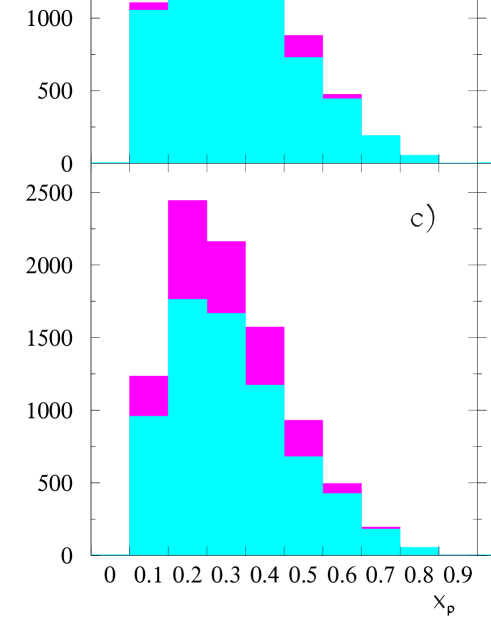
Figure 3: The sample of 17000 events for the $\bar{p}^{\uparrow}\,p^{\uparrow}\rightarrow\mu^{+}\,\mu^{-}\,X$ process where a transversely polarized antiproton beam with energy $E_{\bar{p}}=15$ GeV collides on a transversely polarized proton beam with $E_{p}=3.3$ GeV producing muon pairs of invariant mass $4\leq M\leq 9$ GeV (for further details on the cutoffs, see text). a) $\langle h_{1}(x_{p})\rangle/\langle f_{1}(x_{p})\rangle=\sqrt{x_{p}}$ (brackets mean that each flavor contribution in the numerator is replaced by a common average term, similarly in the denominator; for further details, see text). b) $\langle h_{1}(x_{p})\rangle/\langle f_{1}(x_{p})\rangle=\sqrt{1-x_{p}}$. c) $\langle h_{1}(x_{p})\rangle/\langle f_{1}(x_{p})\rangle=1$. d) $\langle h_{1}(x_{p})\rangle/\langle f_{1}(x_{p})\rangle=0$. For each bin, the darker histogram corresponds to positive values of $\cos(2\phi-\phi_{{}_{S_{\bar{p}}}}-\phi_{{}_{S_{p}}})$ in Eq. (12), the superimposed lighter one to negative values.

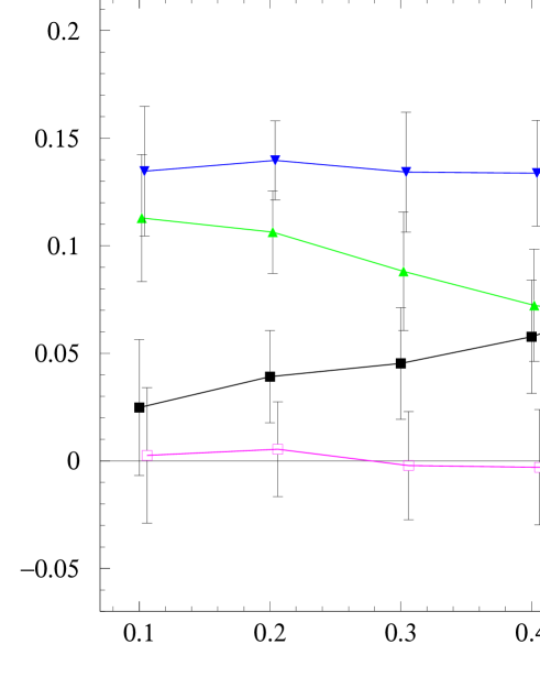
Figure 4: Asymmetry $(U-D)/(U+D)$ between cross sections in the previous figure corresponding to darker histograms ($U$) and superimposed lighter histograms ($D$), as bins in $x_{p}$. Full squares for the case when $\langle h_{1}(x_{p})\rangle/\langle f_{1}(x_{p})\rangle=\sqrt{x_{p}}$, upward triangles when it equals $\sqrt{1-x_{p}}$, downward triangles when it equals 1 and open squares when it equals 0. Continuous lines are drawn to guide the eye. Error bars due to statistical errors only, obtained by 20 independent repetitions of the simulation (see text for further details).

From the above results, we first deduce that the considered sample of events in the specified kinematics is sufficient to produce an average significant asymmetry, at most about 15% for $\langle h_{1}(x_{p})\rangle/\langle f_{1}(x_{p})\rangle=1$. When the ratio equals 0, the corresponding asymmetry consistently oscillates around 0 in all considered bins, also for low $x_{p}$ where the smaller error bars are due to the more dense population of events. In fact, the cross section is known to rapidly increase for decreasing $\tau$ and data accumulate in the part of the phase space corresponding to the lowest possible $\tau$ which, for the considered kinematics, is $\tau\gtrsim 0.08$. At the same time, in the range $0.1\leq x_{p}<0.4$ it seems also that the asymmetries corresponding to the ascending $\sqrt{x_{p}}$ and descending $\sqrt{1-x_{p}}$ functions keep this different behaviour. This means that, although in this limited (but significant) range, it should be possible to extract also information on the analytical dependence of the transversity upon the parton fractional momentum. For higher $x_{p}$ (and $\tau\lesssim 0.4$), the phase space is less populated and the error bars are so large that each one of the four choices for the ratio $\langle h_{1}(x_{p})\rangle/\langle f_{1}(x_{p})\rangle$ can be confused with the other ones.

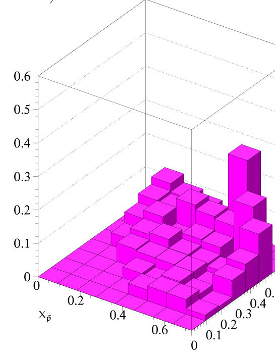
Figure 5: Unintegrated asymmetry $(U-D)/(U+D)$ for the case $\langle h_{1}(x)\rangle/\langle f_{1}(x)\rangle=\sqrt{x}$ in the same conditions as the previous figure, but plotted in bins of $x_{\bar{p}}$ and $x_{p}$. Left panel: distribution of average values. Right panel: distribution of the variances, i.e. of half the statistical ”error bars”, obtained by 20 independent repetitions of the simulation (see text for further details).

This trend is confirmed and better clarified by looking at the unintegrated asymmetry, displayed in Fig. 5 in bins of $x_{\bar{p}}$ and $x_{p}$ for the case $\langle h_{1}(x_{\bar{p}})\rangle\,\langle h_{1}(x_{p})\rangle/\langle f_{1}(x_{\bar{p}})\rangle\,\langle f_{1}(x_{p})\rangle=\sqrt{x_{\bar{p}}}\,\sqrt{x_{p}}$. Namely, it corresponds to the full squares of Fig. 4 for the $x_{\bar{p}}$-integrated case. The left panel represents the bidimensional plot of the average values of the unintegrated double spin asymmetry, while the right panel gives the distribution of the variance, i.e. of half the ”error bar” for each $(x_{\bar{p}},x_{p})$ bin. On the boundaries of the plot, where $x_{\bar{p}},x_{p}$ are close to 1, the small number of collected events produces large statistical errors and also large asymmetries due to fluctuations. Anyway, each bin containing less than 10 events is considered not statistically relevant and the corresponding asymmetry and error have been artificially put to zero. Viceversa, for small $x_{p}\lesssim 0.3$ the variance is small through all the $x_{\bar{p}}$ range so to give a distinguishable integrated double spin asymmetry. Unfortunately, because of the ascending trend of the function $\sqrt{x}$, the absolute values of the asymmetry are small in the $x_{p}$ range of interest, even if statistically different from zero.

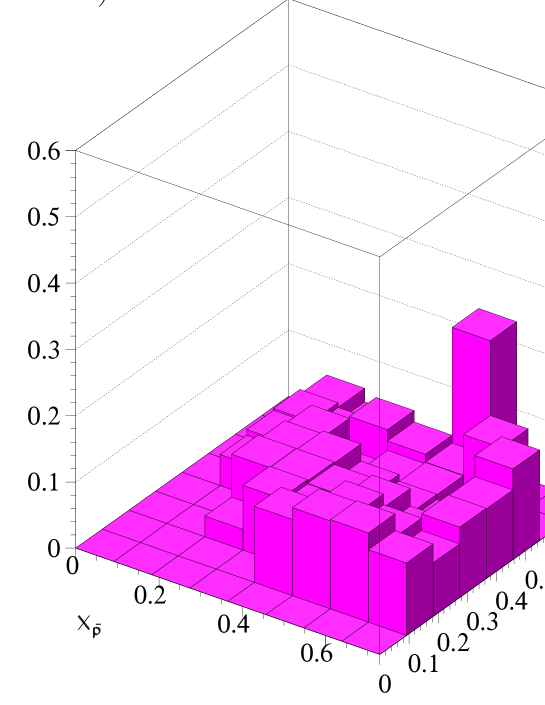
Figure 6: Unintegrated asymmetry $(U-D)/(U+D)$ for the case $\langle h_{1}(x)\rangle/\langle f_{1}(x)\rangle=\sqrt{1-x}$ in the same conditions as the previous figure, plotted in bins of $x_{\bar{p}}$ and $x_{p}$. Left panel: distribution of average values. Right panel: distribution of the variances, i.e. of half the statistical ”error bars”, obtained by 20 independent repetitions of the simulation (see text for further details).

In Fig. 6 the unintegrated double spin asymmetry is displayed for the case $\langle h_{1}(x_{\bar{p}})\rangle\,\langle h_{1}(x_{p})\rangle/\langle f_{1}(x_{\bar{p}})\rangle\,\langle f_{1}(x_{p})\rangle=\sqrt{1-x_{\bar{p}}}\,\sqrt{1-x_{p}}$ in the same conditions as in the previous figure. Therefore, it corresponds to the upward triangles of Fig. 4 for the $x_{\bar{p}}$-integrated case. Similar arguments apply to the statistical selection of the results. The only difference is that for the relevant $x_{p}\lesssim 0.3$ range the absolute values of the asymmetry are more significant because of the descending trend of the function $\sqrt{1-x}$. By comparing the right panel of this figure with the corresponding one in Fig. 5, we notice that errors actually do not depend on the selected test function. They increase with increasing $\tau$, with the exception of some bins that are crossed by the hyperbole $M>4$ GeV/c.

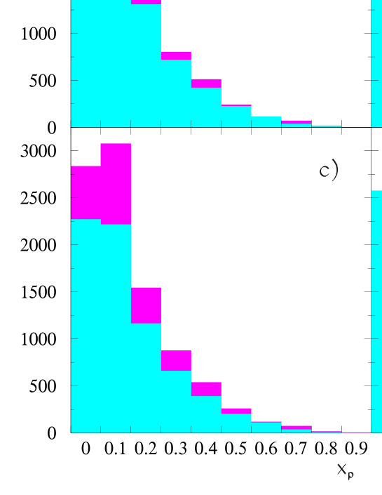
Figure 7: The sample of 17000 events for the $\bar{p}^{\uparrow}\,p^{\uparrow}\rightarrow\mu^{+}\,\mu^{-}\,X$ process for the lepton invariant mass $1.5\leq M\leq 2.5$ GeV, while the other kinematic conditions, conventions for each panel, and color codes of histograms are as in Fig.3 (for further details, see text).

In Fig. (7), the sample of 17000 ”good” events for the $\bar{p}^{\uparrow}\,p^{\uparrow}\rightarrow\mu^{+}\,\mu^{-}\,X$ process is displayed in the same conditions as in Fig. 3, but with the invariant mass of the lepton pair in the range $1.5\leq M\leq 2.5$ GeV. Again, the conventions for the four panels and the color codes of the histograms are the same as in Fig. 3. Since the range of explored $\tau=M^{2}/s$ is now 0.01-0.03, the bins for $x_{p}\rightarrow 0$ are more populated than before, while for $x_{p}>0.7$ yet they are statistically not significant and again they will be discarded in the asymmetry plot.

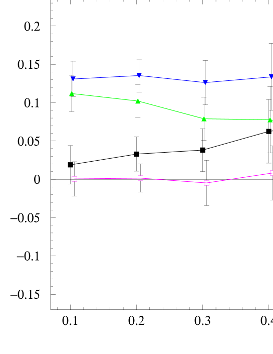
Figure 8: Double spin asymmetry $(U-D)/(U+D)$ between cross sections in the previous figure corresponding to darker histograms ($U$) and superimposed lighter histograms ($D$), as bins in $x_{p}$. Notations as in Fig. 4. Continuous lines are drawn to guide the eye. Error bars due to statistical errors only, obtained by 20 independent repetitions of the simulation (see text for further details).

In Fig. 8, the corresponding double spin asymmetry $(U-D)/(U+D)$ is displayed with the same conventions as in Fig. 4. The larger population for small $x_{p}$ bins reflects in smaller error bars for all four choices of the ratio $\langle h_{1}(x_{p})\rangle/\langle f_{1}(x_{p})\rangle$. Consequently, in the range $0.1\lesssim x_{p}\lesssim 0.3$ the functions $\sqrt{x_{p}}$ (full squares) and $\sqrt{1-x_{p}}$ (upward triangles) are even more distinguishable than in the previous case.

As already recalled in the previous section, we have also explored the typical kinematics suggested by the PANDA collaboration in its proposal at HESR at GSI PANDA Collab. (2004). Namely, the operational mode where the antiproton beam with energy $E_{\bar{p}}=15$ GeV hits a proton target and produces lepton pairs with low invariant masses; we have considered the range $1.5\leq M\leq 2.5$ GeV for the same reasons as above. We have still assumed that the transverse polarization of both beam and target is 50% on the average, such that the corresponding overall dilution factor is 0.25. This corresponds to take $|{\bf S}_{{}_{Tp}}|=|{\bf S}_{{}_{T\bar{p}}}|=1$ in Eqs. (12) and (15) for the 25% of the events, while taking them 0 for the remaining 75%. The resulting cm square energy is $s=30$ GeV² and the range of explored $\tau$ is approximately 0.07-0.2. Consequently, the integrated event distribution of Fig. 9 is more populated at higher $x_{p}$ bins for all the four $\langle h_{1}\rangle/\langle f_{1}\rangle$ ratios explored (notations, conventions and histogram color codes are as in Fig. 3).

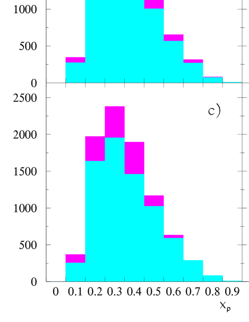
Figure 9: The sample of 17000 events for the $\bar{p}^{\uparrow}\,p^{\uparrow}\rightarrow\mu^{+}\,\mu^{-}\,X$ process where a transversely polarized antiproton beam with energy $E_{\bar{p}}=15$ GeV hits a transversely polarized proton target producing muon pairs with invariant mass $1.5\leq M\leq 2.5$ GeV and $s=30$ GeV². Conventions for each panel and color codes of histograms are as in Fig.3 (for further details, see text).

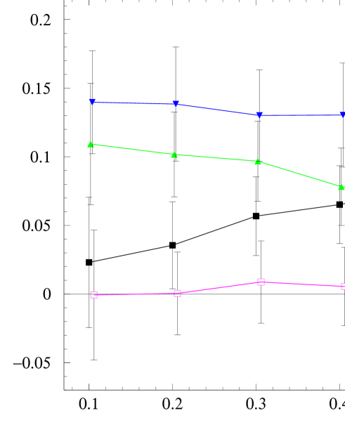
Figure 10: Double spin asymmetry $(U-D)/(U+D)$ between cross sections in the previous figure corresponding to darker histograms ($U$) and superimposed lighter histograms ($D$), as bins in $x_{p}$. Notations as in Fig. 4. Continuous lines are drawn to guide the eye. Error bars due to statistical errors only, obtained by 20 independent repetitions of the simulation (see text for further details).

In Fig. 10, the double spin asymmetry $(U-D)/(U+D)$, corresponding to cross sections of the previous figure, is displayed with the same conventions as in Fig. 4. At variance with the result of Fig. 8, the explored portion of phase space for larger $\tau$ (hence, for larger $x_{p}$ bins) is not favoured by the given $1/\tau$ qualitative dependence of the cross section: a lower density of events reflects in larger statistical error bars which prevent from clearly distinguishing each one of the four considered forms for the $\langle h_{1}\rangle/\langle f_{1}\rangle$ ratio. This means that for the considered sample of 17000 ”good” events, it is not yet clear how to extract information on the analytical structure of $h_{1}(x)$. However, it should be possible at least to observe a nonvanishing asymmetry and give an estimate of its magnitude and sign.

The relevant message of previous figures is that it is crucial to consider integrated distributions in one parton fractional momentum only, in order to reasonably populate bins and to reach a deconvolution of transversity from the product $h(x_{\bar{p}})h(x_{p})$. The price to pay is that the useful phase space in the other fractional momentum is reduced to few bins. It is easy to estimate where the maximum of the distribution is located. Assuming that the bidimensional $(x_{\bar{p}},x_{p})$ distribution is dominated by the $1/\tau$ factor associated with the elementary $q\bar{q}$ fusion into a virtual photon, the distribution is $1/(x_{\bar{p}}x_{p})$ for $\tau>M^{2}_{min}/s$, and 0 otherwise. Consequently, the $x_{\bar{p}}$-integrated distribution has the form $\log(x_{p}s/M^{2}_{min})/x_{p}$ and reaches its peak value for $\log(x_{p}s/M^{2}_{min})=1$, i.e. for $x_{p}=eM_{min}^{2}/s\approx 3M_{min}^{2}/s$. For $M=4$ GeV and $s=200$ GeV², $x_{p}\approx 0.22$ in agreement with Fig. 4. It is evident that it is possible to span the domain of valence contributions for $s$ in the range 100-300 GeV² and $M\gtrsim 4$ GeV. A similar conclusion holds by directly considering the unintegrated distribution, where the relevant contribution of annihilating valence (anti)partons corresponds to $x_{\bar{p}}=x_{p}\approx 0.3$, such that $\tau=x_{p}x_{\bar{p}}\approx 0.1$ can be reached again for $100\lesssim s\lesssim 300$ GeV² and $M\gtrsim 4$ GeV.

Moreover, exploring different masses at the same $s$ (as we did in Figs. 4 and 8) is useful to estimate the role of higher twist effects, since the latter can be classified according to powers of $M/M_{p}$, where $M_{p}$ is the proton mass. However, our results do not include these corrections since precision calculations are beyond the scope of the present work.

In conclusion, it seems that in the collider mode for the HESR at GSI, where the cm square energy is $s=200$ GeV², a sample of 17000 Drell-Yan events from collisions of transversely polarized antiproton and proton beams with proper lepton invariant masses is sufficient to generate sizeable double spin asymmetries from which information can be extracted about the functional dependence of the transversity, but limited to the range $0.1\lesssim x\lesssim 0.3$. For the lower case $s=30$ GeV² in the fixed-target mode, the double spin asymmetry is still sizeable, but the larger statistical error bars do not allow for such a clean extraction.

IV Conclusions

In a previous paper Bianconi and Radici (2004), we produced a Monte Carlo simulation to study the physics case of a Drell-Yan process with unpolarized antiproton beams and transversely polarized proton targets. Here, we have considered the fully polarized $\bar{p}^{\uparrow}\,p^{\uparrow}\rightarrow\mu^{+}\,\mu^{-}\,X$ process in order to explore the leading transverse spin structure of the nucleon. Both works are finalized at the kinematics of the High Energy Storage Ring (HESR), a source for (polarized) antiprotons under development at GSI. In fact, using antiproton beams offers the advantage of involving unsuppressed distributions of valence partons: the transversely polarized quark in a transversely polarized proton, and the transversely polarized antiquark in a transversely polarized antiproton.

Different kinematical options have been considered. Since the cross section fastly decreases for increasing $\tau=M^{2}/s=x_{p}x_{\bar{p}}$ (where $M$ is the lepton pair invariant mass and $s$ is the center-of-mass square energy), events tend to accumulate in the phase space part corresponding to the smallest $\tau$ allowed by the mass cutoff, which is dominated by the valence contribution to parton distributions. It seems convenient to reach such low values of $\tau$ by adequately increasing $s$. The $x_{\bar{p}}$-integrated distributions present a Poisson-like shape in the parton fractional momentum $x_{p}$ with a peak at $x_{p}\approx 3M^{2}_{min}/s$ and width 0.1-0.2. Outside this range, the event distributions are of difficult analysis. For typical $M_{min}$ values, the most interesting $s$ range turns out to be 100-300 GeV², where the possibility of repeating the experiment at different $s$ values allows to analyze different $x_{p}$ ranges.

We have simulated the fully polarized Drell-Yan process using antiproton beams with energy $E_{\bar{p}}=15$ GeV and (transverse) polarization 50%, and proton beams with the same polarization and energy $E_{p}=3.3$ GeV, such that $s=200$ GeV². To avoid the $c\bar{c}$ threshold and other resonances in the mass spectrum of the lepton pair, we selected the invariant mass $M$ in the ranges 4-9 GeV and 1.5-2.5 GeV. The corresponding explored $\tau$ ranges are 0.08-0.4 and 0.01-0.03, respectively. We have also explored the case where the transversely polarized antiproton beam of 15 GeV hits a transversely polarized fixed proton target producing lepton pairs with invariant mass in the same range 1.5-2.5 GeV. In this case, $s=30$ GeV² and the $\tau$ range is approximately 0.07-0.2. The mass range 4-9 GeV has not been considered here, because it implies average $x_{p}$ values where the parton model underlying the simulation is not appropriate.

In all cases, the transverse momentum of the dimuon couple has been limited to $q_{{}_{T}}>1$ GeV/$c$ and its zenithal-angle distribution is restricted to the range 60-120 deg. The former cut is induced by the need to avoid complicated soft mechanisms and to match the experimental requirements of the collider setup. The latter cut prevents the angular dependence of the cross section from diluting the related asymmetry. All these cuts produce a remarkable reduction of the Drell-Yan events: the considered initial sample of 80000 events (only affected by the mass cut) is reduced to 17000.

At leading twist in the cross section, the contribution of interest has a characteristic azimuthal dependence of the kind $\cos(2\phi-\phi_{{}_{S_{\bar{p}}}}-\phi_{{}_{S_{p}}})$, where $\phi$ is the azimuthal angle of the final lepton pair and $\phi_{{}_{S_{p(\bar{p})}}}$ is the azimuthal position of the (anti)proton transverse spin in the Collins-Soper frame. Hence, for each randomly distributed $\phi_{{}_{S_{\bar{p}}}}$ events have been accumulated for parallel $(\phi_{{}_{S_{\bar{p}}}}=\phi_{{}_{S_{p}}})$ and antiparallel $(\phi_{{}_{S_{\bar{p}}}}=\phi_{{}_{S_{p}}}+\pi)$ beam polarizations. The corresponding azimuthal asymmetry has been built either integrating upon all variables but the quark fractional momentum $x_{p}$, or keeping also the corresponding antiquark $x_{\bar{p}}$ dependence and building bidimensional plots.

For each kinematical case, we have considered four functional dependences for the transversity, each one with a very peculiar trend, namely constant, ascending, descending, and zero, but all satisfying the Soffer bound. The goal is to recover the same different trend also in the corresponding double spin asymmetry, which means that feasibility conditions for an unambiguous extraction of the transversity could be established. In the collider mode with $s=200$ GeV², the double spin asymmetry has very small statistical error bars for $0.1\lesssim x_{p}\lesssim 0.3$. With this limitation, it seems that a sample of 17000 events satisfying all the described cutoffs, should be sufficient to grant the identification of the analytical behaviour of the transversity. This statement is still valid at the lower $M$ range considered by keeping the same $s$, because the resulting $\tau$ range is shifted to lower values and the statistics is higher. Viceversa, for the option where the antiproton beam hits a fixed proton target, a lower $s$ results in larger error bars: measuring a nonvanishing double spin asymmetry seems possible, but the extraction of the transversity looks more problematic.

In conclusion, with the present simulation we have explored the feasibility conditions for an unambiguous extraction of the transversity from Drell-Yan data with polarized antiproton beams; we hope to have contributed to the studies of the physics case for hadronic collisions with antiproton beams at the HESR at GSI.

References

- Artru and Mekhfi (1990) X. Artru and M. Mekhfi, Z. Phys. C45, 669 (1990).
- Jaffe and Ji (1991) R. L. Jaffe and X. Ji, Phys. Rev. Lett. 67, 552 (1991).
- Jaffe (1996) R. L. Jaffe (1996), proceedings of the Ettore Majorana International School on the Spin Structure of the Nucleon, Erice, Italy, 3-10 Aug 1995., eprint [http://arXiv.org/abs]hep-ph/9602236.
- Barone and Ratcliffe (2003) V. Barone and P. G. Ratcliffe, Transverse Spin Physics (World Scientific, River Edge, USA, 2003).
- Aoki et al. (1997) S. Aoki, M. Doui, T. Hatsuda, and Y. Kuramashi, Phys. Rev. D56, 433 (1997), eprint hep-lat/9608115.
- Jaffe and Ji (1993) R. L. Jaffe and X. Ji, Phys. Rev. Lett. 71, 2547 (1993), eprint [http://arXiv.org/abs]hep-ph/9307329.
- Ralston and Soper (1979) J. P. Ralston and D. E. Soper, Nucl. Phys. B152, 109 (1979).
- Martin et al. (1998) O. Martin, A. Schafer, M. Stratmann, and W. Vogelsang, Phys. Rev. D57, 3084 (1998), eprint hep-ph/9710300.
- Barone et al. (1997) V. Barone, T. Calarco, and A. Drago, Phys. Rev. D56, 527 (1997), eprint hep-ph/9702239.
- Mulders and Tangerman (1996) P. J. Mulders and R. D. Tangerman, Nucl. Phys. B461, 197 (1996), erratum-ibid. B484 (1996) 538, eprint [http://arXiv.org/abs]hep-ph/9510301.
- Collins (1993) J. C. Collins, Nucl. Phys. B396, 161 (1993), eprint [http://arXiv.org/abs]hep-ph/9208213.
- Sivers (1990) D. W. Sivers, Phys. Rev. D41, 83 (1990).
- Gamberg et al. (2003) L. P. Gamberg, G. R. Goldstein, and K. A. Oganessyan, Phys. Rev. D68, 051501 (2003), eprint hep-ph/0307139.
- Bacchetta et al. (2004) A. Bacchetta, A. Schaefer, and J.-J. Yang, Phys. Lett. B578, 109 (2004), eprint hep-ph/0309246.
- Efremov et al. (2003) A. V. Efremov, K. Goeke, and P. Schweitzer, Phys. Lett. B568, 63 (2003), eprint hep-ph/0303062.
- Anselmino et al. (2005) M. Anselmino, M. Boglione, U. D’Alesio, E. Leader, and F. Murgia, Phys. Rev. D71, 014002 (2005), eprint hep-ph/0408356.
- Brodsky et al. (2002) S. J. Brodsky, D. S. Hwang, and I. Schmidt, Phys. Lett. B530, 99 (2002), eprint [http://arXiv.org/abs]hep-ph/0201296.
- Belitsky et al. (2003) A. V. Belitsky, X. Ji, and F. Yuan, Nucl. Phys. B656, 165 (2003), eprint hep-ph/0208038.
- Burkardt and Hwang (2004) M. Burkardt and D. S. Hwang, Phys. Rev. D69, 074032 (2004), eprint hep-ph/0309072.
- Collins and Ladinsky (1994) J. C. Collins and G. A. Ladinsky (1994), eprint [http://arXiv.org/abs]hep-ph/9411444.
- Bacchetta and Radici (2004a) A. Bacchetta and M. Radici, Phys. Rev. D70, 094032 (2004a), eprint hep-ph/0409174.
- Bacchetta and Radici (2003) A. Bacchetta and M. Radici, Phys. Rev. D67, 094002 (2003), eprint hep-ph/0212300.
- Bacchetta and Radici (2004b) A. Bacchetta and M. Radici, Phys. Rev. D69, 074026 (2004b), eprint hep-ph/0311173.
- Bianconi et al. (2000) A. Bianconi, S. Boffi, R. Jakob, and M. Radici, Phys. Rev. D62, 034008 (2000), eprint [http://arXiv.org/abs]hep-ph/9907475.
- Radici et al. (2002) M. Radici, R. Jakob, and A. Bianconi, Phys. Rev. D65, 074031 (2002), eprint [http://arXiv.org/abs]hep-ph/0110252.
- Jaffe et al. (1998) R. L. Jaffe, X. Jin, and J. Tang, Phys. Rev. Lett. 80, 1166 (1998), eprint [http://arXiv.org/abs]hep-ph/9709322.
- Bravar (2000) A. Bravar (Spin Muon), Nucl. Phys. A666, 314 (2000).
- Airapetian et al. (2004) A. Airapetian et al. (HERMES) (2004), eprint [http://arXiv.org/abs]hep-ex/0408013.
- PAX Collab. (2004) PAX Collab., Letter of Intent for Antiproton-Proton Scattering Experiments with Polarization, Spokespersons: F. Rathmannn and P. Lenisa (2004), http://www.fz-juelich.de/ikp/pax/.
- Lenisa et al. (2004) P. Lenisa et al. (PAX) (2004), eprint hep-ex/0412063.
- ASSIA Collab. (2004) ASSIA Collab., Letter of Intent for A Study of Spin-dependent Interactions with Antiprotons: the Structure of the Proton, Spokesperson: R. Bertini (2004), http://www.gsi.de/documents/DOC-2004-Jan-152-1.ps.
- Maggiora (2005) M. Maggiora (ASSIA) (2005), eprint hep-ex/0504011.
- Efremov et al. (2004) A. V. Efremov, K. Goeke, and P. Schweitzer, Eur. Phys. J. C35, 207 (2004), eprint hep-ph/0403124.
- Anselmino et al. (2004) M. Anselmino, V. Barone, A. Drago, and N. N. Nikolaev, Phys. Lett. B594, 97 (2004), eprint hep-ph/0403114.
- Bianconi and Radici (2004) A. Bianconi and M. Radici, Phys. Rev. D71, 074014 (2004), eprint hep-ph/0412368.
- Boer (1999) D. Boer, Phys. Rev. D60, 014012 (1999), eprint hep-ph/9902255.
- Falciano et al. (1986) S. Falciano et al. (NA10), Z. Phys. C31, 513 (1986).
- Guanziroli et al. (1988) M. Guanziroli et al. (NA10), Z. Phys. C37, 545 (1988).
- Conway et al. (1989) J. S. Conway et al., Phys. Rev. D39, 92 (1989).
- Collins and Soper (1977) J. C. Collins and D. E. Soper, Phys. Rev. D16, 2219 (1977).
- Boer and Mulders (1998) D. Boer and P. J. Mulders, Phys. Rev. D57, 5780 (1998), eprint [http://arXiv.org/abs]hep-ph/9711485.
- Tangerman and Mulders (1995) R. D. Tangerman and P. J. Mulders, Phys. Rev. D51, 3357 (1995), eprint [http://arXiv.org/abs]hep-ph/9403227.
- Brandenburg et al. (1993) A. Brandenburg, O. Nachtmann, and E. Mirkes, Z. Phys. C60, 697 (1993).
- Brandenburg et al. (1994) A. Brandenburg, S. J. Brodsky, V. V. Khoze, and D. Muller, Phys. Rev. Lett. 73, 939 (1994), eprint hep-ph/9403361.
- Eskola et al. (1994) K. J. Eskola, P. Hoyer, M. Vanttinen, and R. Vogt, Phys. Lett. B333, 526 (1994), eprint hep-ph/9404322.
- PANDA Collab. (2004) PANDA Collab., Letter of Intent for the Proton-Antiproton Darmstadt Experiment, Spokesperson: U. Wiedner (2004), http://www.gsi.de/documents/DOC-2004-Jan-115-1.pdf.
- Anassontzis et al. (1988) E. Anassontzis et al., Phys. Rev. D38, 1377 (1988).
- Altarelli et al. (1979) G. Altarelli, R. K. Ellis, and G. Martinelli, Nucl. Phys. B157, 461 (1979).
- Buras and Gaemers (1978) A. J. Buras and K. J. F. Gaemers, Nucl. Phys. B132, 249 (1978).
- Soffer (1995) J. Soffer, Phys. Rev. Lett. 74, 1292 (1995), eprint [http://arXiv.org/abs]hep-ph/9409254.