Unitarity constraints on top quark
signatures of Higgsless models

Abstract

We use conditions for unitarity cancellations to constrain the couplings of the top and bottom quarks to Kaluza-Klein modes in Higgsless models of electroweak symmetry breaking. An example for the mass spectrum of quark resonances in a theory space model is given and the implications for the collider phenomenology in the top sector are discussed, comparing to signatures of Little Higgs and strong electroweak symmetry breaking models.
PACS Numbers: 12.15.-y, Electroweak interactions; 14.65.Ha,Top quarks; 11.10.Kk, Field theories in dimensions other than four; 11.15.Ex, Spontaneous breaking of gauge symmetries

1 Introduction

Recently it has been suggested that a viable description of electroweak symmetry breaking (EWSB) without a Higgs boson, weakly coupled up to energies of $\Lambda=5$-$10$ TeV, may be achieved employing gauge symmetry breaking by boundary conditions in a higher dimensional spacetime [1]. Variants of the setup in a warped or flat extra dimension [2] and four dimensional ‘theory space’ models [3, 4, 5] have been constructed. The mechanism of gauge symmetry breaking by boundary conditions has been investigated from several perspectives [6, 7] and applied to extended gauge symmetries and six dimensional models [8]. The basic idea of the higher dimensional Higgsless models is to cure the bad high energy behavior of scattering amplitudes of massive gauge bosons by the exchange of Kaluza-Klein (KK)-excitations of the electroweak gauge bosons. The relevant unitarity cancellations are ensured by higher dimensional gauge invariance [1, 6, 9] or by a large number of sites in theory space models [10]. A cutoff scale $\Lambda$—reflecting the non-renormalizable nature of the higher dimensional gauge theory—is implied by partial wave unitarity bounds [9, 10, 11] resulting from the increasing number of open channels.

Fermion masses in 5D Higgsless models can be generated by allowing the fermions to propagate in the extra dimension and introducing appropriate boundary localized kinetic and mass terms [12] which is consistent with unitarity cancellations as long as the reduced gauge symmetry at the boundaries is respected by the localized terms [13].

Early phenomenological studies of the five dimensional models considered fermions localized near a brane and found it difficult to accommodate electroweak precision data [14, 15] while raising the cutoff scale significantly compared to four dimensional strongly interacting models [11], in agreement with theory space results [4, 5]. However, as pointed out subsequently [16, 17] the delocalization of the fermions in the extra dimension or analogous theory space constructions [18, 19, 20] allows to suppress the couplings of the light fermions to the KK-gauge bosons and might be the key for a realistic model.

While no fully realistic model has emerged yet, recent studies [21, 22] concentrate on signatures of the mechanism of Higgsless EWSB in gauge boson scattering at the CERN Large Hadron Collider (LHC). To identify generic signatures in this channel, ref. [22] utilizes the conditions for unitarity cancellations [1, 6] to constrain the couplings of the gauge boson KK-resonances. The aim of the present work is to constrain signatures of Higgsless models in the top quark sector using a similar approach. We show that the KK-excitations of the third family quarks are also a generic feature of a Higgsless model which remains perturbative up to a scale $\Lambda\approx 5$-$10$ TeV, although the detailed structure of the mass spectrum and the coupling constants is more model dependent than in gauge boson scattering.

The large top quark mass implies that the third family quarks play a special role in Higgsless models, for instance it appears difficult to delocalize the third family in the same way as the lighter fermions [16]. In addition, it has been argued [16] that precision electroweak constraints on the $Zb\bar{b}$ vertex require the first KK-excitations of the third family quarks to be considerably heavier than the gauge boson KK-modes. In this context it is interesting to recall the Appelquist-Chanowitz (AC) unitarity bound [23, 24] $\Lambda_{t}=8\pi v^{2}/(\sqrt{2N_{c}}m_{t})\sim 3.5$ TeV on the the scale of mass generation for the top quark (we have used the slightly tighter bound given recently by Dicus and He in [24]). Hence there is a potential tension between the AC bound and large masses of top-quark KK-modes. On the other hand, this bound suggests that signals of the mechanism of mass generation are more likely to be observable in the third family quarks than for lighter fermions, especially if the light fermions are delocalized and decouple from the gauge boson KK-modes.

In section 2 we review previous results on third family quarks in 5D Higgsless models and give an example for the mass spectrum of the KK bottom and top quarks in a theory space model. In section 3 we will present the sum rules ensuring the boundedness of the 4 particle scattering amplitudes involving third family quarks. Based on this sum rules, in section 4 we introduce a simple scenario for the first KK-level of gauge bosons and third family quarks in a Higgsless model and comment on the resulting collider phenomenology, comparing it to that of the heavy top quark in Little Higgs models and of heavy gauge bosons in models of strong EWSB.

2 Third family quarks in Higgsless models

In this section we recall different possibilities for the fermionic sector of Higgsless models and the resulting KK-spectrum in the top quark sector (For convenience, the term ‘KK-mode’ will be used also in theory space models). After a short overview over 5D models, in subsection 2.1 a simple theory space model is discussed in some more detail. While it is beyond the scope of the present work to construct a fully realistic model, this section provides us with an example for a mass spectrum of the KK modes that will be used for purposes of illustration later on. Some aspects of the top quark sector in Higgsless models with a warped extra dimension have been discussed in [14, 16].

Let us briefly recall the setup of 5D models and the features of the fermion mass spectrum. The models of [1, 2] employ a left-right symmetric bulk gauge group $SU(2)_{L}\otimes SU(2)_{R}\otimes U(1)$. The same group structure is also used in warped models including a Higgs scalar [25]. Flavor physics in these models has been discussed in [26]. On the brane at $y=\pi R\equiv\ell$ the left-right symmetry is broken to the diagonal subgroup $SU(2)_{L+R}$, on the second brane at $y=0$ the symmetry breaking pattern is $SU(2)_{R}\otimes U(1)\to U(1)_{Y}$. Left- and right-handed fermions arise as zero modes of bulk $SU(2)_{L}$ and $SU(2)_{R}$ doublets $\Psi_{L}$ and $\Psi_{R}$, respectively.

Without additional structure, the zero mode fermions are massless and there are degenerate Dirac-KK modes for the left- and right-handed fermions. To give masses to the zero modes, Dirac masses consistent with the unbroken $SU(2)_{L+R}$ can be added on the brane at $y=\ell$ [12]. To obtain a mass splitting between the up and down type quarks, two different possibilities have been considered. In [12] the right-handed up- and down type quarks are contained in the same bulk $SU(2)_{R}$ doublet $\Psi_{R}$. To lift the mass degeneracy in the isospin multiplets, one can use the $y=0$ brane where the broken $SU(2)_{R}$ allows to add boundary kinetic terms for the right handed down-type quarks. The large boundary term needed in this setup to obtain the mass splitting between the top and bottom quark also results in a large mass splitting of the first KK-modes of bottom and top quark. In the setup of [25] also used in a Higgsless model in [14], two $SU(2)_{R}$ doublets $\Psi^{t}_{R}$ and $\Psi^{b}_{R}$ are introduced that contain the right-handed top and bottom quarks as zero modes. This allows to use different brane masses for top and bottom quarks at $y=\ell$ so no large boundary kinetic term is needed to split the isospin doublets. Additional structure must be added on the $y=0$ brane to give large masses to the unwanted down-type zero mode of $\Psi^{t}_{R}$ and the up-type zero mode of $\Psi^{b}_{R}$.

The large boundary mass term necessary for the top quark mass splits the initially degenerate KK-modes of $\Psi_{L}$ and $\Psi_{R}$. In a flat extra-dimension, the splitting turns out to be similar to the brane mass itself, in a warped extra dimension the effects can be even larger depending on the localization of the zero mode fermions [14, 27]. Thus, in this setup the mass of the lightest top quark KK-mode is likely to be significantly lighter than that of the gauge bosons. Since perturbativity in gauge boson scattering requires the gauge boson KK-modes to be as light as possible [11], the first KK-mode of the top quark would therefore be dangerously light. In the setup with $t_{R}$ and $b_{R}$ in the same bulk doublet $\Psi_{R}$ [12], the large boundary kinetic term needed to get the top-bottom mass splitting will make the first bottom KK-mode even lighter, while in the setup with separate $\Psi^{t}_{R}$ and $\Psi^{b}_{R}$ doublets, one expects only a small mass splitting of the bottom KK-modes. Furthermore, reference [16] finds a tension in obtaining a large enough top mass while obeying constraints on the $Zbb$ vertex and concludes that in a realistic warped 5D model the masses in the top quark sector must be generated by a separate mechanism. This tension is reduced if one allows the gauge boson KK-modes to become heavier by giving up the demand for perturbativity up to $5$-$10$ TeV [14]. Also warped models including a a Higgs scalar [25, 26] and with the first gauge boson KK level at $3$-$4$ TeV are less affected by this problem.

2.1 Theory space setup

As an example for a theory space Higgsless model including delocalized fermions, we consider the ‘one-site delocalized’ setup of ref. [18] that performed a numerical analysis for a 4-site model. We will now extend this simple model to include right-handed fermions and generate fermion masses. We thus consider a $SU(2)^{3}\otimes U(1)$ gauge theory with $3$ nonlinear sigma models with symmetry breaking pattern $SU(2)\otimes SU(2)/SU(2)$ acting as link fields. The link fields $U_{i}$ transform under the gauge transformations as

$$U_{i}\to g_{i-1}^{\dagger}U_{i}g_{i}$$ (2.1)

where $i\in\{1,2,3\}$. Here for $i<3$ the gauge transformations $g_{i}$ are elements of $SU(2)_{i}$ while for $i=3$ there is only a $U(1)$ gauge transformation.

In [18] a left handed fermion doublet $\psi_{L}=(\psi_{t,L},\psi_{b,L})$ is introduced on the site $i=0$ and a doublet of vector-like fermions $\Psi_{1}$ on the second site $i=1$. Both have the same Hypercharge and therefore are charged under the $U(1)$ on site $3$. The continuum limit will be similar to the setup of [17] based on a single bulk $SU(2)$ where also non-local couplings of the fermions to the unbroken $U(1)$ located on one boundary have to be introduced. Avoiding this nonlocality in theory space requires additional $U(1)$ groups, corresponding to a faithful deconstruction of the 5D $SU(2)_{R}\otimes SU(2)_{L}\otimes U(1)$ 5D model [4] which will not be considered in the following. To give mass to the standard model (SM) fermions, we will additionally include two right-handed fermions $\chi_{bR}$ and $\chi_{tR}$ on the $U(1)$ site, with the same Hypercharges as the right-handed SM up- and down-type quarks. Finally, a second vector-like doublet $\Psi_{2}$ is introduced at the site $i=2$. A gauge invariant Lagrangian is given by

$$-\mathcal{L}_{M}=M_{\Psi 1}\bar{\Psi}_{1L}\Psi_{1R}+M_{\Psi 2}\bar{\Psi}_{2L}\Psi_{2R}+y_{1}f_{1}\bar{\psi}_{L}U_{1}\Psi_{1R}+y_{2}f_{2}\bar{\Psi}_{1L}U_{2}\Psi_{2R}\\ +y_{3}f_{3}\bar{\Psi}_{2L}U_{3}(\lambda^{0}+\lambda^{3}\sigma^{3})\chi_{R}+\,\text{h.c.}$$ (2.2)

where the notation $\chi_{R}=(\chi_{tR},\chi_{bR})$ has been introduced. Here ‘nonlocal’ gauge invariant terms involving products of the link fields have been discarded. They are usually argued to be generated by higher order effects only and therefore suppressed. The mass matrix for the top quark sector is given by

$$-\mathcal{L}_{M_{t}}=\begin{pmatrix}\bar{\psi}_{t},&\bar{\Psi}_{t1},&\bar{\Psi}_{t2}\end{pmatrix}_{L}\begin{pmatrix}f_{1}y_{1}&0&0\\ M_{\Psi 1}&f_{2}y_{2}&0\\ 0&M_{\Psi 2}&f_{3}y_{t}\end{pmatrix}\begin{pmatrix}\Psi_{t1}\\ \Psi_{t2}\\ \chi_{t}\end{pmatrix}_{R}+\,\text{h.c.}$$ (2.3)

with $y_{t}=y_{3}(\lambda^{0}+\lambda^{3})$. The matrix for the bottom sector differs only in the third entry on the diagonal that is instead given by $y_{b}=y_{3}(\lambda^{0}-\lambda^{3})$.

For the ‘one-site delocalized’ model without $\chi_{R}$ and $\Psi_{2}$, there is a massless zero mode $\psi_{L}^{(0)}=(\cos\theta_{\Psi 1}\psi_{L}-\sin\theta_{\Psi 1}\Psi_{1L})$ with $\sin\theta_{\Psi 1}=f_{1}y_{1}/\sqrt{(f_{1}y_{1})^{2}+M_{\Psi 1}^{2}}$. Applying this setup to the light fermions, good agreement with electroweak precision data was found in [18] for the parameters $f_{1}=300$ GeV and $f_{2}=f_{3}=592$ GeV and a mixing angle $\sin^{2}\theta_{\Psi 1}=0.01477$ that translates into

$$M_{\Psi_{1}}=\frac{f_{1}y_{1}}{\tan\theta_{\Psi 1}}=y_{1}\times 2450\,\text{GeV}$$ (2.4)

while the masses of the KK gauge boson are given by [18] $m_{W^{(1)}}\sim m_{Z^{(1)}}\sim 890$ GeV. Remarkably, already in this simple model the ‘KK excitation’ $\psi_{L}^{(1)}=(\sin\theta_{\Psi 1}\psi_{L}+\cos\theta_{\Psi 1}\Psi_{1L})$ has a mass of $m_{\psi^{(1)}}=\sqrt{(y_{1}f_{1})^{2}+M_{\Psi 1}^{2}}=y_{1}\times 2.5$ TeV and is naturally heavier than the gauge boson KK-modes. For purposes of illustration, we use the same input parameters for our extended setup for the third family quarks. As an example for a mass spectrum where the mass splitting of the first top and bottom quark masses is not too large, for the parameters $y_{1}=1.5$, $y_{2}=4$, $y_{t}=5$, $y_{b}=0.08$ and choosing $M_{\Psi 1}=M_{\Psi 2}$ as in (2.4) one obtains the spectrum

$$m_{t} =178.7\,\text{GeV} m_{T^{1}} =3.1\,\text{TeV} m_{T^{2}} =5.6\,\text{TeV}$$ (2.5)

$$m_{b} =4.6\,\text{GeV} m_{B^{1}} =2.5\,\text{TeV} m_{B^{2}} =5.5\,\text{TeV}$$

In contrast to the five dimensional setup, there are no almost degenerate KK-modes in this model. From the eigenvectors of the square of the mass matrix in (2.2) one finds that—because of the large Yukawa coupling $y_{t}$—the right handed top-quark zero mode has a considerable admixture of $\Psi_{t1/2,R}$ while the other zero modes are approximately ‘localized’ on the sites $0$ and $3$. Such a composite structure of the right-handed top is also expected in warped 5D models, where the right-handed top quark has to be localized near the brane where EWSB takes place [14, 16, 26]. Thus, corrections to the right-handed top quark couplings seem to be another generic prediction of the class of Higgsless models considered here, in addition to the direct signatures of the KK-modes that are the focus of the remainder of this work.

3 Unitarity cancellations in the top quark sector

To introduce our method and to present results needed in the following, we briefly review the unitarity bounds on the couplings of the KK-gauge bosons to the $W$ and $Z$ obtained in [22]. The cancellation of terms growing like $E^{4}$ and $E^{2}$ in the $WZ\to WZ$ and $W^{+}W^{-}\to W^{+}W^{-}$ scattering amplitudes implies the sum rules (see also [1, 28, 6])

$$3\sum_{n}g^{2}_{ZWW^{(n)}}m^{2}_{W^{(n)}} =g^{2}_{ZWW}\frac{m_{Z}^{4}}{m_{W}^{2}}$$ (3.1)

$$3\sum_{n}g_{WWZ^{(n)}}^{2}m_{Z^{(n)}}^{2} =\left(4m_{W}^{2}-3m_{Z}^{2}\right)g_{WWZ}^{2}+4m_{W}^{2}g_{WW\gamma}^{2}$$

up to terms suppressed by an order of $(m_{W}/m_{W^{(}n)})^{2}$. Therefore upper bounds [22] on the interaction of the $W$ and $Z$ KK-modes can be obtained:

$$g_{ZWW^{(1)}} \lesssim\frac{g_{ZWW}m_{Z}^{2}}{\sqrt{3}m_{W^{(1)}}m_{W}}\overset{\text{SM}}{=}\frac{gm_{Z}}{\sqrt{3}m_{W^{(1)}}}$$ (3.2)

$$g_{WWZ^{(1)}} \overset{\text{SM}}{\lesssim}\frac{gm_{W}}{\sqrt{3}m_{Z^{(1)}}}$$

We have indicated the result of inserting the tree level SM values for the zero mode couplings. One expects corrections to these values in Higgsless models [1] but the SM values will be used for purposes of illustration. In the remainder of this section, the relations corresponding to (3.1) in the top-quark sector are discussed, the constraints on the coupling constants corresponding to (3.2) will be subject of section 4.

3.1 Unitarity sum rules for third family quarks

Consider the scattering of zero mode fermions, denoted by $q_{i}$, and zero mode vector bosons, denoted by $V_{a}$, that couple to the corresponding KK-modes $Q_{i}^{(n)}$ and $V_{a}^{(n)}$. We will only be concerned with interactions that involve a single KK-excitation and parameterize the corresponding interaction Lagrangian as

$$\mathcal{L}_{\text{int}}=\sum_{n}\Bigl{\{}\mathrm{i}g_{V_{a}V_{b}V_{c}^{(n)}}\partial^{\mu}V_{a}^{\nu}V_{b\mu}V_{c\nu}^{(n)}\\ +\left[g^{L/R}_{i(j,n)V_{a}}\bar{q}_{i}\mathchoice{\ooalign{$\hfil\displaystyle\mkern 0.0mu/\hfil$\crcr$\displaystyle V$}}{\ooalign{$\hfil\textstyle\mkern 0.0mu/\hfil$\crcr$\textstyle V$}}{\ooalign{$\hfil\scriptstyle\mkern 0.0mu/\hfil$\crcr$\scriptstyle V$}}{\ooalign{$\hfil\scriptscriptstyle\mkern 0.0mu/\hfil$\crcr$\scriptscriptstyle V$}}_{a}\left(\tfrac{1\pm\gamma^{5}}{2}\right)Q_{j}^{(n)}+g^{L/R}_{ijV_{a}^{(n)}}\bar{q}_{i}\mathchoice{\ooalign{$\hfil\displaystyle\mkern 0.0mu/\hfil$\crcr$\displaystyle V$}}{\ooalign{$\hfil\textstyle\mkern 0.0mu/\hfil$\crcr$\textstyle V$}}{\ooalign{$\hfil\scriptstyle\mkern 0.0mu/\hfil$\crcr$\scriptstyle V$}}{\ooalign{$\hfil\scriptscriptstyle\mkern 0.0mu/\hfil$\crcr$\scriptscriptstyle V$}}_{a}^{(n)}\left(\tfrac{1\pm\gamma^{5}}{2}\right)q_{j}\right]+\,\text{h.c.}\Bigr{\}}$$ (3.3)

where we have included the zero modes in the sums by defining $Q^{(0)}_{i}=q_{i}$ and similarly for the vector bosons. A sum over the internal quantum numbers is implied. With the convention of (3.3), in the SM we have for instance $g_{ZW^{+}W^{-}}=g\cos\theta_{w}$ where $g=2m_{W}/v$ is the weak coupling constant.

The unitarity sum rules for this situation can be obtained in a straightforward way from the results of [28] by omitting the Higgs contributions and allowing for an infinite number of intermediate particles. The cancellation of the leading divergences $\propto E^{2}$ in the scattering $\bar{q}_{i}q_{k}\to V_{a}V_{b}$ is ensured by the sum rule.

$$\sum_{n,j}\left[g^{L/R}_{i(j,n)V_{a}}g^{L/R}_{(j,n)kV_{b}}-g^{L/R}_{i(j,n)V_{b}}g^{L/R}_{(j,n)kV_{a}}\right]=\sum_{n,c}g_{V_{a}V_{b}V_{c}^{(n)}}g^{L/R}_{ikV_{c}^{(n)}}$$ (3.4a)

This is just the generalization of the Lie algebra $$[\tau^{a},\tau^{b}]=\mathrm{i}f^{abc}\tau^{c} \tau^{a} f^{abc} \propto E$$ that holds in a gauge theory where the fermions live in a representation of the gauge group generated by the and the structure constants enter the triple gauge boson vertex. This relation therefore is not associated with the symmetry breaking mechanism. In contrast, for the cancellation of the subleading divergences usually a Higgs boson is invoked. In absence of Higgs scalars, this sum rule takes the form

$$\sum_{n,j}m_{q_{i}}g^{L}_{i(j,n)V_{b}}g^{L}_{(j,n)kV_{a}}+m_{q_{k}}g^{R}_{i(j,n)V_{a}}g^{R}_{(j,n)kV_{b}}-m_{q_{j}^{(n)}}\left(g^{R}_{i(j,n)V_{b}}g^{L}_{(j,n)kV_{a}}+g^{R}_{i(j,n)V_{a}}g^{L}_{(j,n)kV_{b}}\right)\\ =\sum_{c,n}\frac{(m_{V_{a}}^{2}-m_{V_{b}}^{2}-m_{V_{c}^{(n)}}^{2})}{2m_{V_{c}^{(n)}}^{2}}g_{V_{a}V_{b}V_{c}^{(n)}}\left(m_{q_{i}}g^{L}_{ikV_{c}^{(n)}}-m_{q_{k}}g^{R}_{ikV_{c}^{(n)}}\right)$$ (3.4b)

and the same equation with left- and right-handed couplings exchanged. It can be shown that in the special case of identical fermions and bosons as external particles, the right-handed version of (3.4b) is not an independent condition but is satisfied identically after (3.4a) is used, in agreement with a result of Gunion et.al in [28].

The relations (3.4) are a consequence of the underlying higher dimensional gauge symmetry and can consequently also be obtained from the Ward Identities of the theory [6]. As verified in [6, 13], these relations are left intact by gauge symmetry breaking by Dirichlet boundary conditions and boundary terms for the fermions consistent with the reduced gauge symmetry on the brane. Similar to the case of gauge boson scattering [10], it is expected that the unitarity cancellations work approximately for a large number of sites in theory space models.

We now will evaluate the sum rules (3.4) for processes involving the third family quarks and the $W$ and $Z$ bosons. The KK-modes of the bottom and top quarks will be denoted as $T^{(n)}$ and $B^{(n)}$. In a 5D model, there can be separate towers of vector-like KK-modes for the left-handed and right-handed quarks but for notational simplicity, we will not introduce a different notation for these towers. The $b$ quark is treated as massless everywhere and frequently axial couplings $g^{A}=\frac{1}{2}(g_{R}-g_{L})$ are used.

For the processes $W^{+}W^{-}\to t\bar{t}$ and $W^{+}W^{-}\to b\bar{b}$ the condition (3.4a) gives

$$-(g^{L/R}_{Wtb})^{2}+g_{ZWW}g_{ttZ}^{L/R}+g_{WW\gamma}g_{tt\gamma} =\sum_{n}\left[(g^{L/R}_{WtB^{(n)}})^{2}-g_{WWZ^{(n)}}g_{ttZ^{(n)}}^{L/R}\right]\overset{\text{SM}}{=}0$$ (3.5a)

$$(g^{L/R}_{Wtb})^{2}+g_{ZWW}g_{bbZ}^{L/R}+\mathrm{i}g_{WW\gamma}g_{bb\gamma} =-\sum_{n}\left[(g^{L/R}_{WT^{(n)}b})^{2}+g_{WWZ^{(n)}}g_{bbZ^{(n)}}^{L/R}\right]\overset{\text{SM}}{=}0$$ (3.5b)

The sign change in the relation for bottom quarks arises since a different term in the Lie algebra (3.4a) contributes. In the following, we will concentrate on the sum rule for top quarks, the case of bottom quarks is similar. As indicated, the expressions on the left hand side vanish if the tree level SM values are inserted, reflecting the fact that these relations are a consequence of gauge invariance alone, independent of the mechanism of EWSB. Note however, that many top quark couplings are presently constrained only indirectly by experiment, for instance by assuming unitarity of the Cabibbo-Kobayashi-Maskawa matrix. In a Higgsless model the couplings of the zero modes will in general receive corrections compared to the SM. In particular, as mentioned in section 2 one expects modified couplings of the right-handed top quark, arising from localization towards the EWSB brane in 5D models or from a large Yukawa coupling on the $U(1)_{Y}$ site in theory space models. The condition for the cancellation of the subleading divergences (3.4b) results in

$$(g^{L}_{Wtb})^{2}+g_{ZWW}g_{ttZ}^{A}=\sum_{n}\Biggl{[}\tfrac{m_{B^{(n)}}}{m_{t}}g^{R}_{WtB^{(n)}}g^{L}_{WtB^{(n)}}-(g^{L}_{WtB^{(n)}})^{2}-g_{WWZ^{(n)}}g_{ttZ^{(n)}}^{A}\Biggr{]}$$ (3.6)

Subtracting the left- and right-handed versions of (3.5) and using (3.6) one can eliminate the $Ztt$ couplings :

$$(g^{L}_{Wtb})^{2}+(g^{R}_{Wtb})^{2}=\sum_{n}\left[2\tfrac{m_{B^{(n)}}}{m_{t}}g^{R}_{WtB^{(n)}}g^{L}_{WtB^{(n)}}-(g^{L}_{WtB^{(n)}})^{2}-(g^{R}_{WtB^{(n)}})^{2}\right]$$ (3.7)

Note that the disappearance of the couplings of the $Z$-KK-modes from the sum rule implies that the unitarity cancellations cannot be achieved by including only vector boson resonances and the presence of fermion KK-modes is necessary.

Following [22] we should now proceed to obtain an upper bound on the $g_{WtB^{(1)}}$ coupling by saturating the sum rule (3.7) by the first resonance. However, in principle individual terms of the sum (3.7) can be negative if the left-and right-handed couplings are very different. On the other hand, for the higher KK-modes this becomes increasingly unlikely because the positive contribution is enhanced by the KK-mass. Hence we expect that a bound similar to (3.2) can safely be obtained from the sum rule (3.7) in a scenario with a non-degenerate KK-spectrum as in the theory space model discussed in section 2. Introducing the notation $g^{L}_{WqQ^{(1)}}=\sqrt{2}\sin\theta_{Q}g_{WqQ^{(1)}}$ and $g^{R}_{WqQ^{(1)}}=\sqrt{2}\cos\theta_{Q}g_{WqQ^{(1)}}$ one then obtains

$$(g^{L}_{Wtb})^{2}\gtrsim 2g_{WtB^{(1)}}^{2}\left(\tfrac{m_{B^{(1)}}}{m_{t}}\sin 2\theta_{B}-1\right)$$ (3.8)

In contrast to the case of gauge boson scattering considered in [22], this bound is not model independent but involves the relation of right-and left-handed couplings. We will solve the sum rules derived in this section under the assumption of a non-degenerate spectrum and saturation by the first KK-level in the next section. For almost degenerate KK-excitations of the $b$ quark as in some $SU(2)_{L}\otimes SU(2)_{R}\otimes U(1)$ 5D models, in principle there can be cancellations among the degenerate modes and more detailed knowledge of the chiral structure of the couplings would be necessary to exploit the sum rules.

Turning now to the process $ZZ\to t\bar{t}$, in this case the sum rule (3.4a) is satisfied trivially, since there is no coupling of three neutral gauge bosons, even involving KK modes. The remaining relation (3.4b) gives

$$4\left(g_{ttZ}^{A}\right)^{2}=-\sum_{n}\left[\left(g_{tT^{(n)}Z}^{L}\right)^{2}+\left(g_{tT^{(n)}Z}^{R}\right)^{2}-2\tfrac{m_{T^{(n)}}}{m_{t}}g_{tT^{(n)}Z}^{R}g_{tT^{(n)}Z}^{L}\right]\overset{\text{SM}}{=}\frac{g^{2}}{4\cos^{2}\theta_{W}}$$ (3.9)

Finally, there are the sum rules for $W^{+}Z\to\bar{b}t$ that have a more involved form than those considered previously:

$$\begin{split}(g_{ttZ}^{L/R}&-g_{bbZ}^{L/R}-g_{ZWW})g_{Wtb}^{L/R}\\ &=-\sum_{n}\Biggl{[}g_{tT^{(n)}Z}^{L/R}g_{WT^{(n)}b}^{L/R}-g_{bB^{(n)}Z}^{L/R}g_{WtB^{(n)}}^{L/R}-g_{ZWW^{(n)}}g_{W^{(n)}tb}^{L/R}\Biggr{]}\overset{\text{SM}}{=}0\end{split}$$ (3.10a)

$$\begin{split}&-\left(2g_{ttZ}^{A}+\tfrac{m_{Z}^{2}}{2m_{W}^{2}}g_{ZWW}\right)g_{Wtb}^{L}\\ &=\sum_{n}\Biggl{[}(\tfrac{m_{T^{(n)}}}{m_{t}}g_{tT^{(n)}Z}^{R}-g_{tT^{(n)}Z}^{L})g_{WT^{(n)}b}^{L}+\tfrac{m_{B^{(n)}}}{m_{t}}g_{WtB^{(n)}}^{R}g_{bB^{(n)}Z}^{L}+\tfrac{1}{2}g_{W^{(n)}tb}^{L}g_{ZWW^{(n)}}\Biggr{]}\overset{\text{SM}}{=}0\end{split}$$ (3.10b)

where the second equation holds up to terms of the order $m_{W}^{2}/m^{2}_{W^{(n)}}$. In this case, the condition with left- and right-handed couplings exchanged gives an independent condition. The only new couplings appearing in these relations are the coupling of the $W$-KK modes $g_{W^{(n)}tb}$. Combining both relations of (3.10) results in the consistency relation

$$0\overset{\text{SM}}{=}\sum_{n}\left(2\tfrac{m_{T^{(n)}}}{m_{t}}g_{tT^{(n)}Z}^{R}-g_{tT^{(n)}Z}^{L}\right)g_{WT^{(n)}b}^{L}+\left(2\tfrac{m_{B^{(n)}}}{m_{t}}g_{WtB^{(n)}}^{R}-g_{WtB^{(n)}}^{L}\right)g_{bB^{(n)}Z}^{L}$$ (3.11)

The sum rules derived in this section are sufficient to ensure that the matrix elements for four-particle processes with external SM particles remain bounded at large energies. For a fully consistent model, in addition to the interaction considered in (3.3) also coupling constants among the KK-modes have to be taken into account, satisfying the appropriate sum rules to cancel unitarity violations in the scattering amplitudes of the KK-resonances [1]. Furthermore despite cancellation of the terms growing with the energy, eventually partial wave unitarity will be violated by the growing multiplicity of open channels [9, 11].

4 Implications for collider phenomenology

Obtaining generic predictions from the unitarity sum rules derived in the last section is less straightforward than in gauge boson scattering considered in [22]. With some further input from model-building or some simplifying assumptions, however, these relations can be useful to constrain the interactions of the first KK-level of a Higgsless model. This is demonstrated in subsection 4.1 for a simple setup with a non-degenerate mass spectrum. In subsection 4.2 we give examples for the high energy behavior of some four particle cross sections in this scenario and study the effects of varying the KK-masses and coupling constants. In subsection 4.3 we compare our scenario to top-sector signatures of Little Higgs models and general vector resonances in models of strong EWSB.

4.1 Minimal Higgsless scenario for the first KK-level

In the following all zero-mode couplings will be approximated by their tree-level SM value (implicitly also done in [22]) and it is assumed that the sum rules are saturated by the first resonance. It is straightforward to allow for deviations of the zero mode couplings from their SM values, we comment on this briefly below. Almost degenerate KK-resonances of the quarks will not be considered, as discussed in section 2 this corresponds to theory space models of the type considered in [18] or the continuum limit as in [17]. Under these assumptions, the sum rules derived in section 3 can be solved so that all four point amplitudes of the SM fermions and gauge bosons remain bounded at high scattering energies. A unitarization of four point amplitudes with external particles from the first KK-level would require the inclusion of higher KK levels [1]. The scenario described in this section has been implemented into the multi-purpose event-generator O’Mega/WHIZARD [29].

In the following, the explicit analytic expressions of the coupling constants in terms of masses and SM couplings will be displayed only for the case of equal left-and right handed couplings. As argued in subsection 4.2 below, the deviations from this limit should remain small in order to keep the cross sections significantly beyond the SM predictions in the $m_{H}\to\infty$ limit up to $\sqrt{s}=5$ TeV. In our implementation in O’Mega, the left-and right-handed couplings are kept as free input parameters and the exact formulas resulting from the sum rules are used. Ambiguities in the absolute signs of the coupling constants will be fixed to satisfy the constraint (3.11).

Considering (3.8) in the vector-like limit $\theta_{Q}=\pi/4$ and inserting the SM value $g^{L}_{Wtb}=g/\sqrt{2}$ gives:

$$g_{WqQ^{(1)}}^{L/R}\approx\frac{g}{2}\sqrt{\frac{m_{q}}{m_{Q^{(1)}}}}$$ (4.1)

Similarly, from the sum rules (3.5) from $W^{+}W^{-}\to q\bar{q}$ one obtains, truncating after the first KK-level and using the SM value for the zero mode couplings:

$$g_{qqZ^{(1)}}^{L/R}=(-)^{\chi_{q}}\frac{(g_{WqQ^{(1)}}^{L/R})^{2}}{g_{WWZ^{(1)}}}=(-)^{\chi_{q}}\frac{\sqrt{3}g}{4}\frac{m_{q}m_{Z^{(1)}}}{m_{W}m_{Q^{(1)}}}$$ (4.2)

with $\chi_{t}=0$ and $\chi_{b}=1$. The neutral current coupling of the quark resonances is given from (3.9) as

$$g_{qQ^{(1)}Z}^{L/R}\approx\sqrt{\frac{2m_{q}}{m_{Q^{(1)}}}}g^{A}_{qqZ}=(-)^{\chi_{q}+1}\frac{g}{2\cos\theta_{w}}\sqrt{\frac{m_{q}}{2m_{Q^{(1)}}}}$$ (4.3)

The remaining coupling $g_{W^{(1)}tb}$ can be fixed using (3.10a):

$$g_{W^{(1)}tb}^{L/R}=\frac{1}{g_{ZWW^{(1)}}}(g_{tT^{(1)}Z}^{L/R}g_{WT^{(1)}b}^{L/R}-g_{bB^{(1)}Z}^{L/R}g_{WtB^{(1)}}^{L/R})\approx-\frac{gm_{W^{(1)}}}{2m_{B^{(1)}}m_{W}}\sqrt{\frac{3}{2}m_{t}m_{b}}$$ (4.4)

where the last expression holds provided $m_{T^{(1)}}\approx m_{B^{(1)}}$. Finally, under the condition that the terms proportional to the KK-masses dominate, the consistency condition (3.11) simplifies to

$$m_{T^{(1)}}g_{tT^{(1)}Z}^{R}g_{WT^{(1)}b}^{L}=-m_{B^{(1)}}g_{WtB^{(1)}}^{R}g_{bB^{(1)}Z}^{L}$$ (4.5)

which is satisfied for our sign conventions used above. For deviations from the vector-like limit, this condition and the one obtained by exchanging left- and right-handed couplings constrains the ratios of left-and right handed couplings, leaving us with two additional free parameters. Together with the triple gauge boson couplings (3.2), these results provide a simple description for the first KK-level of a Higgsless model.

Let us briefly discuss the impact of modified zero mode couplings. Consider a non-vanishing right-handed $Wtb$ coupling, parameterized as $g^{R}_{Wtb}=\frac{g}{\sqrt{2}}\epsilon_{R}$. From (3.5), (3.7) and (3.10a) we obtain the relative changes in the couplings (4.1), (4.2) and (4.4) as

$$\frac{\delta g_{WtB^{(1)}}^{L/R}}{g_{WtB^{(1)}}^{L/R}}\approx\frac{\epsilon_{R}^{2}}{2}\qquad,\qquad\frac{\delta g_{ttZ^{(1)}}^{R}}{g_{ttZ^{(1)}}^{R}}\approx\frac{m_{B^{(1)}}}{m_{t}}\epsilon_{R}^{2}\qquad,\qquad\frac{\delta g_{W^{(1)}tb}^{R}}{g_{W^{(1)}tb}^{R}}\approx\frac{2m_{B^{(1)}}}{\sqrt{m_{t}m_{b}}}\epsilon_{R}$$ (4.6)

A non-vanishing right-handed $Wtb$ coupling therefore gives only small corrections to the couplings of the quark KK-modes while the couplings of the $Z$ boson KK-modes can be enhanced moderatly for instance $\epsilon_{R}=5\%$ results in $\delta g_{ttZ^{(1)}}^{R}/g_{ttZ^{(1)}}^{R}\approx 4\%$ for $m_{B^{(1)}}=3$ TeV. In contrast, large changes can arise in the couplings of the KK-modes of the $W$ boson.

We are now in the position to determine the decay widths of the KK particles. The partial decay widths for $W^{(1)}\to WZ$ [22] and $Z^{(1)}\to W^{+}W^{-}$ are given by

$$\Gamma_{W^{(1)}\to WZ} \approx\frac{g_{W^{(1)}WZ}^{2}}{48\pi}\frac{m^{5}_{W^{(1)}}}{4m_{W}^{2}m_{Z}^{2}}\lesssim\frac{\alpha_{\mathrm{QED}}m_{W^{(1)}}^{3}}{144\sin^{2}\theta_{w}m_{W}^{2}}$$ (4.7)

$$\Gamma_{Z^{(1)}\to WW} \approx\frac{g_{WWZ^{(1)}}^{2}}{48\pi}\frac{m^{5}_{Z^{(1)}}}{4m_{W}^{4}}\lesssim\frac{\alpha_{\mathrm{QED}}m_{Z^{(1)}}^{3}}{144\sin^{2}\theta_{w}m_{W}^{2}}$$

For $m_{W^{(1)}}=m_{Z^{(1)}}=700$ GeV the numerical value is approximately $13$ GeV. For vector-like couplings, the partial decay width of the heavy $Z$ into top-quarks is given by

$$\Gamma_{Z^{(1)}\to t\bar{t}}\approx\frac{g^{2}_{ttZ^{(1)}}m_{Z^{(1)}}}{4\pi}\approx\frac{3\,\alpha_{\mathrm{QED}}m^{3}_{Z^{(1)}}}{16\sin^{2}\theta_{w}m_{W}^{2}}\left(\frac{m_{t}}{m_{B^{(1)}}}\right)^{2}=27\left(\frac{m_{t}}{m_{B^{(1)}}}\right)^{2}\Gamma_{Z^{(1)}\to W^{+}W^{-}}$$ (4.8)

For $m_{B^{(1)}}=2.5$ TeV the numerical value is about $14\%$ of the $Z^{(1)}\to W^{+}W^{-}$ branching ratio but for $m_{B^{(1)}}=1$ TeV it becomes as large as $86\%$. As can be seen from (4.4), the fermionic branching ratio of the $W^{(1)}$ $\Gamma_{W^{(1)}\to t\bar{b}}$ is suppressed compared to that of the $Z^{(1)}$ by a factor $m_{b}/m_{t}$.

The partial decay widths of the heavy quarks into SM particles are

$$\Gamma_{Q^{(1)}\to qZ} \approx\frac{g_{Q^{(1)}qZ}^{2}}{16\pi}\frac{m_{Q^{(1)}}^{3}}{m_{Z}^{2}}=\frac{\alpha_{\mathrm{QED}}}{32\sin^{2}\theta_{w}\cos^{2}\theta_{w}}\frac{m_{q}m_{Q^{(1)}}^{2}}{m_{Z}^{2}}$$ (4.9)

$$\Gamma_{Q^{(1)}\to qW} \approx\frac{g_{Q^{(1)}qW}^{2}}{16\pi}\frac{m_{Q^{(1)}}^{3}}{m_{W}^{2}}=\frac{\alpha_{\mathrm{QED}}}{16\sin^{2}\theta_{w}}\frac{m_{q}m_{Q^{(1)}}^{2}}{m_{W}^{2}}$$

The dominant decay channels are hence the neutral current decay for the $T^{(1)}$ and the charged current decay for the $B^{(1)}$ that are not suppressed by the small $b$-quark mass. For $m_{T^{(1)}}=m_{B^{(1)}}=1$ TeV we find $\Gamma_{T^{(1)}\to tZ}\approx 30$ GeV and $\Gamma_{B^{(1)}\to tW}\approx 60$ GeV. The dependence on $m_{Q}^{2}$ leads to a rapid growth with the mass, for instance $m_{T^{(1)}}=3$ TeV and $m_{B^{(1)}}=2.5$ TeV lead to $\Gamma_{T^{(1)}\to tZ}\approx 270$ GeV and $\Gamma_{B^{(1)}\to tW}\approx 380$ GeV. Note that for such large masses also decays like $Q^{(1)}\to Z^{(1)}q$ are kinematically allowed. In a 5D theory with a flat extra dimension compactified on an orbifold, the corresponding KK-number conserving coupling constants are of the same order of magnitude as the zero mode couplings, whereas couplings involving a single KK mode are suppressed since they are generated only by KK-parity violating boundary terms. While we have not worked out the unitarity constraints for the KK-number conserving coupling constants, we expect they are not suppressed by factors $\mathcal{O}(\sqrt{(m_{q}/m_{Q})})$. We estimate the order of magnitude for the partial decay width for these channels by $\Gamma_{T^{(1)}\to tZ^{(1)}}\sim(m_{T^{(1)}}m_{Z}^{2})/(m_{t}m_{Z^{(1)}}^{2})\Gamma_{T^{(1)}\to tZ}\sim 0.3\Gamma_{T^{(1)}\to tZ}$ for $m_{T^{(1)}}=3$ TeV. While this simple argument suggests that the decay to one KK-mode and a zero mode is subdominant, this point can only be settled within a concrete model.

4.2 High energy-behavior of cross sections

We now give results for the cross sections $W^{+}W^{-}\to t\bar{t}$ and $ZZ\to t\bar{t}$ in the scenario discussed in the previous subsection. This serves on one hand to demonstrate that our choice of coupling constants indeed implements the required unitarity cancellations and leads to decreasing cross sections at high energies. On the other hand, we address the question whether one can safely raise the KK-masses of the third family quarks near the AC-bound while significantly improving the high energy behavior compared to the SM in the limit of an infinite Higgs mass. We also discuss whether the couplings can be raised significantly compared to the values discussed above, either by deviating from vector-like couplings or by violating the sum rules.

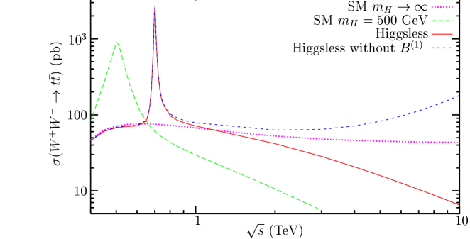
Figure 1: Cross section for $W^{+}W^{-}\to t\bar{t}$ in the SM with a Higgs resonance, the SM in the $m_{H}\to\infty$ limit and the Higgsless scenario with $m_{Z}^{(1)}=700$ GeV and $m_{B^{(1)}}=2.5$ TeV

In figure 1 the cross section for $W^{+}W^{-}\to t\bar{t}$ is shown in various scenarios. As expected, in the SM in the limit of an infinite Higgs mass the cross section tends to a constant at high energies, corresponding to a scattering matrix element growing linearly with the energy. Both in the SM with a Higgs resonance (for comparison with the Higgsless model, a rather heavy Higgs with $m_{H}=500$ GeV is shown in this plot, but the high energy limit is the same for a lighter Higgs) and in the Higgsless scenario the scattering matrix element is bounded at large energies and the cross section decreases. However, in the Higgsless scenario this decrease sets in at much higher energies than in the SM. It has been checked, that this behavior is not improved for smaller $m_{Z^{(1)}}$. As emphasized previously, the improved high energy behavior in the Higgsless scenario is due to the heavy $B$ quark. Indeed, as can be seen in figure 1 and in agreement with the sum rule (3.5), the inclusion of a single $Z$ resonance without a heavy $B$ rather destroys the unitarity cancellations present in the SM and leads to a growing cross section at high energies (for comparison the couplings of the $Z^{(1)}$ have been taken as in (4.2) with $m_{B^{(1)}}=2.5$ TeV).

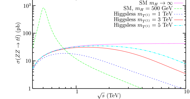
Figure 2: Cross section for $ZZ\to t\bar{t}$ in the SM with a Higgs resonance, the SM in the $m_{H}\to\infty$ limit and the Higgsless SM for three different masses of the heavy top.

Figure 2 shows the cross section for the process $ZZ\to t\bar{t}$ for three different values of $m_{T^{(1)}}$. Here no resonance appears in the Higgsless model so the unitarization is entirely due to the top quark KK-mode. It can be seen that that the numerical value of the cross section at large energies is determined by the mass of the $T^{(1)}$ since the unitarity cancellations become effective earlier on for a lower mass. For $m_{T^{(1)}}=1$ TeV the cross section is suppressed considerable compared to the $m_{H}\to\infty$ limit of the SM already for $\sqrt{s}$= 2 TeV. At $\sqrt{s}$= 3.5 TeV the cross section remains about $20\%$ below the infinite Higgs mass limit for masses up to $5$ TeV. The situation is similar for $W^{+}W^{-}\to t\bar{t}$. While a partial wave analysis as in [9, 10, 11] is required to arrive at definite conclusions, this result indicates that it should be possible to raise the mass of the KK-modes of the top and bottom quarks as seems to be required by low energy constraints without running in conflict with unitarity.

The explicit expressions for the coupling constants like (4.1) and (4.3) hold only if the difference between left- and right-handed couplings is not too large. One observes from (3.8) that in principle the coupling constants can be enhanced by a factor $(\sin 2\theta_{B}-m_{t}/m_{B^{(1)}})^{-1}$. On the other hand, this also increases the cross section so that the demand to do better than the SM in the infinite Higgs mass limit at $\sqrt{s}=\Lambda_{t}=3.5$ TeV places a bound on the ratio $g_{WtB^{(1)}}^{L}/g_{WtB^{(1)}}^{R}=\tan\theta_{B}$. From figure 3 one can see that this implies $\tan\theta_{B}\gtrsim 0.4$, corresponding to an enhancement of $g_{WtB^{(1)}}$ by a factor of $1.6$ compared to (4.1). Therefore the relations (4.1) and (4.3) will not be corrected by large numbers, if one insists on a better high energy behavior than in the SM with $m_{H}\to\infty$.

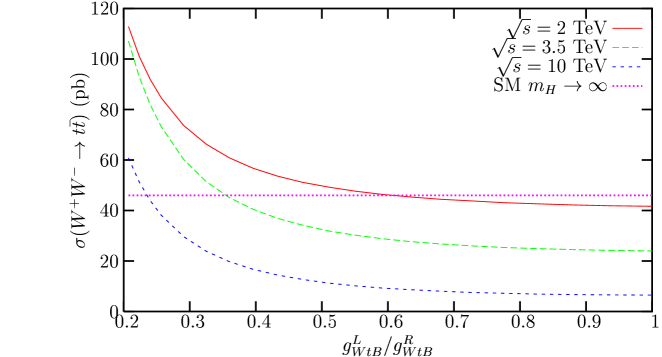
Figure 3: Cross section for $WW\to t\bar{t}$ for a varying ratio of left-and right handed $WtB^{(1)}$ couplings while keeping the bound (3.8) saturated.

Another interesting question concerns the effect of small violations of the unitarity sum rules on the high energy behavior of the cross section. For the example of the $W^{+}W^{-}\to t\bar{t}$ cross section, figure 4 shows the effect of varying the $WtB^{(1)}$ coupling while keeping the remaining couplings fixed. As a first observation, one notes that the coupling constant derived in subsection 4.1 indeed is ‘optimal’ in the sense that the cross section has the smallest value in the high energy limit. For smaller energies, however, the ‘optimal’ coupling is shifted to larger values, indicating that the cancellations induced by the heavy $B$ quark become more effective earlier on for an increased coupling, while in the high energy limits the cancellations are spoiled. Depending on the cutoff scale $\Lambda\sim 5$-$10$ TeV of the theory induced by perturbativity in gauge boson scattering, the coupling $g_{WtB}$ might be raised at most to $1.2$-$1.4$ times the value inferred from (4.1).

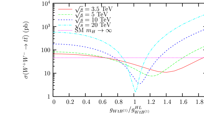
Figure 4: Dependence of the $WW\to t\bar{t}$ cross section on the $WtB^{(1)}$ coupling where $g^{HL}_{WtB^{(1)}}$ denotes the value (4.1). The remaining couplings are kept fixed.

4.3 Comparison with other EWSB scenarios

Let us now compare our scenario with the collider phenomenology of fermion or vector boson resonances in the top sector that have been considered in the context of Little Higgs models [30, 31] or strong EWSB [32, 33]. We first turn to the top-quark signals of the gauge boson KK-modes before we discuss the KK-modes of the third family quarks.

Signals of a $1$ TeV vector resonance in the vector boson fusion process $W^{+}W^{-}\bar{t}t$ were studied in [32] for an $e^{+}e^{-}$ linear collider operating at $\sqrt{s}=1.5$ TeV. From the results of the second reference in [32] one finds that this process is suitable for probing the partial widths in the region $\Gamma_{Z^{(1)}\to W^{+}W^{-}}\gtrsim 10$ TeV and $\Gamma_{Z^{(1)}\to t\bar{t}}\gtrsim 2.4$ TeV with a precision of $13\%$ for a luminosity of $200\,\text{fb}^{-1}$. The bosonic decay width is of the expected magnitude in our scenario, for the fermionic decay width of the $Z^{(1)}$ (4.8), this region corresponds to masses $m_{B^{(1)}}\lesssim 2.2$ TeV. A high energy linear collider therefore should be suitable to probe the coupling of the third family quarks to the KK-modes of the gauge bosons and might even provide a check on the unitarity sum rules.

Concerning hadron collider signatures, it was found that at the LHC the detection of resonances in $W^{+}W^{-}\to\bar{t}t$ is overwhelmed by QCD background [33]. Recently, the second reference in [33] considered a different scenario with a neutral gauge boson coupling predominantly to the third generation of quarks with the coupling to gauge bosons and light fermions suppressed. The associated production of a heavy vector boson with $b$ or $t$ quarks, for instance in single top production $Wb\to tZ^{(1)}$ or in bottom or top pair production $gg\to t\bar{t}Z^{(1)}$ has been found to be the most useful signature. For a partial decay width $\Gamma_{Z^{(1)}\to t\bar{t}}=63$ GeV this reference finds a $5\sigma$ significance at the LHC for masses up to $m_{Z^{(1)}}=2$ TeV. In our scenario the partial decay width of the heavy $Z$ to top quarks is only about $4\%-17\%$ of the value considered in [33], depending on $m_{B^{(1)}}$. However, for $m_{Z^{(1)}}<1$ TeV—as expected from unitarity in gauge boson scattering—the cross sections of the channels considered in [33] grow rapidly so one expects that they are useful also in the context of Higgsless models. Clearly, a more careful study in the scenario described in 4.1 is needed to arrive at definite conclusions, for instance the total cross section for $W^{+}W^{-}\to t\bar{t}$ at high energies (c.f. figure 1) is by construction much smaller than in the scenarios with a single vector resonance considered in [32, 33].

While the detection of the KK-resonances of the gauge bosons would provide evidence for the nature of the mechanism of gauge symmetry breaking, the KK-resonances of the top and bottom quark are connected to the mechanism of mass generation of the quarks and might help to distinguish 5D from theory space models. The production of heavy top quarks at the LHC has been studied recently in the context of Little Higgs models [30, 31]. In the so called Littlest Higgs model [34], the couplings of the heavy top $T$ are suppressed compared to that of the top quark by a mixing angle given approximately by [30] $\lambda_{1}m_{t}/(\lambda_{2}m_{T})$ where the ratio of Yukawa couplings $\lambda_{1}$ and $\lambda_{2}$ is usually taken to be of the order one. For $\lambda_{1}/\lambda_{2}=1$, the discovery reach of the LHC for the heavy top has been estimated [31] as $m_{T}=2$ TeV for the production in $W$-$b$ fusion $qb\to q^{\prime}T$ and the decay channel $T\to Wb$. In comparison to our result (4.9), the total decay width of the heavy top in the Littlest Higgs model is given by [30]

$$\Gamma_{T}^{\text{LH}}\approx\frac{\alpha_{\mathrm{QED}}m_{T}m_{t}^{2}}{8\sin^{2}\theta_{w}m_{W}^{2}}\left(\frac{\lambda_{1}}{\lambda_{2}}\right)^{2}=\frac{4m_{t}}{m_{T}}\left(\frac{\lambda_{1}}{\lambda_{2}}\right)^{2}\Gamma^{\text{HL}}_{T^{(1)}\to tZ}$$ (4.10)

with branching ratios given by [30] $\text{Br}(T\to bW)=50\%$ and $\text{Br}(T\to tZ)=\text{Br}(T\to tH)=25\%$. Recall from (4.9) that the decay $T^{(1)}\to bW$ is suppressed by a factor $2m_{b}/m_{t}\sim 5\%$ in the Higgsless scenario. Thus for $m_{T^{(1)}}=1$ TeV the heavy top has $\Gamma_{T}^{LH}=22$ GeV in the Littlest Higgs model and is moderately narrower than in the Higgsless scenario. In contrast, for $m_{T}=3$ TeV the heavy top remains relatively narrow in the little Higgs model with $\Gamma_{T}^{LH}=62$ TeV while the width is over four times larger in the Higgsless scenario. On the other hand, the charged coupling constants involved in the production of the heavy top are given by $g_{WTb}^{L}=\frac{g}{\sqrt{2}}\frac{m_{t}\lambda_{1}}{m_{T}\lambda_{2}}$ compared to our result (4.1). Noting that the relevant quantity is the sum of the squared left-and right-handed couplings, the production cross section in the Littlest Higgs model and the Higgsless scenario will be related by

$$\sigma_{\text{LH}}(Wb\to T)=\frac{m_{t}^{2}}{m_{b}m_{T}}\left(\frac{\lambda_{1}}{\lambda_{2}}\right)^{2}\sigma_{\text{HL}}(Wb\to T^{(1)})$$ (4.11)

For $m_{T}=1$ TeV, the cross section in the Higgsless scenario corresponds to that in the Little Higgs scenario for $\lambda_{2}=2.7\lambda_{1}$. In this mass region, the phenomenology of the heavy top hence is similar to that in the Littlest Higgs model, albeit for a slightly pessimistic point in parameter space. For $m_{T}=3$ TeV this improves to $\lambda_{2}=1.6\lambda_{1}$ but in this mass region the heavy top is already a rather broad resonance so its phenomenology will be even more challenging than in the Littlest Higgs model.

The heavy bottom quark is a feature distinguishing the Higgsless scenario from (minimal implementations of) Little Higgs models. Here the charged current coupling is enhanced by the top quark mass, unfortunately the production in the $s$-channel process $q\bar{q}\to W^{-}\to B^{(1)}\bar{t}$ is kinematically suppressed at LHC energies. Another possible production channel, neutral current $bZ$ fusion $qb\to qB^{(1)}$ suffers from the suppressed neutral current coupling, so the situation is similar as for the heavy top quark.

One could also consider the production of the heavy quarks by QCD processes. In Little Higgs models, strong pair production of the heavy top quark has found to be kinematically suppressed compared to the weak process of single $T$ production [30]. Strong effects might be more relevant in higher dimensional models where there are also effects of the KK-modes of the gluons (see e.g. [25]) that, however, are not special to Higgsless models and cannot be constrained in our approach. If the KK-modes of the top and bottom quark evade direct detection at the LHC, effects of quark mixing with the KK-modes may only be observable by indirect effects on the top quark gauge couplings [35].

5 Summary and outlook

In the spirit of a recent analysis of gauge boson scattering in generic Higgsless models [22], we have constrained the interactions in the top sector of Higgsless models by unitarity sum rules. While the KK-resonances of the bottom and top quarks are essential for good high energy behavior of scattering amplitudes involving the top quark, electroweak precision constraints in a 5D Higgsless model suggest that they must be significantly heavier than the gauge boson KK-modes [16]. In section 2 we have seen that this can be achieved more naturally in theory-space models than in 5D models.

Although a larger number of coupling constants is involved compared to gauge boson scattering discussed in [22], the sum rules presented in section 3 constrain the parameter space significantly. In section 4 we have solved them in the approximation that only the first KK-level contributes and for a non-degenerate mass spectrum as in the theory space model discussed in section 2. A numerical analysis of the cross section for $W^{+}W^{-}\to t\bar{t}$ in this scenario has shown that the coupling constants can only deviate from the values given in section 4.1 by a limited amount if the high energy behavior is to improve significantly compared to the SM in the $m_{H}\to\infty$ limit. It will be interesting to compare the top sector of a realistic theory space or higher dimensional Higgsless model to the scenario discussed in section 4.

The collider phenomenology of the gauge boson KK-modes in our setup has some features in common with certain models of strong EWSB where vector resonances couple predominantly to the third generation [32, 33] while the feature of a excited top quark with mass $m_{T}=1$-$3$ TeV is shared by Little Higgs models. Comparison with results of [32, 33] suggests that the coupling of the first $Z$ boson KK-mode to the top quark can be probed in $t\bar{t}$ production via vector boson fusion at a high energy linear collider [32] and in associated production with top quarks at the LHC [33]. The phenomenology of the top and bottom quark KK-modes is more challenging since the charged current interactions of the heavy top and the neutral current interactions of the heavy bottom are suppressed by the small mass of the bottom quark. If the top and bottom quark KK-modes indeed have to be significantly heavier than that of the gauge bosons, as suggested in [16], they will be difficult to detect at the LHC. The scenario described in section 4 has been implemented into the multi-purpose event-generator O’Mega/WHIZARD, allowing for more detailed phenomenological studies in the future.

Note added:

After the submission of this paper, ref [36] appeared that discusses a model for the third family quarks based on two slices of $AdS_{5}$ space. In this setup scalar ”top-pions” appear and the KK-resonances of the top and bottom quark are in the $6-7$ TeV region. The top-sector is either strongly coupled or a a ”Top-Higgs” is introduced, restoring unitarity in $W^{+}W^{-}\to t\bar{t}$ scattering. In contrast, the present work considered a top sector that remains perturbative without introduction of a scalar boson.

References

- [1] C. Csáki et al. Phys. Rev. D69 (2004) 055006 [hep-ph/0305237]
- [2] C. Csáki, C. Grojean, L. Pilo, and J. Terning Phys. Rev. Lett. 92 (2004) 101802 [hep-ph/0308038]; Y. Nomura JHEP 11 (2003) 050 [hep-ph/0309189]; R. Barbieri, A. Pomarol, and R. Rattazzi Phys. Lett. B591 (2004) 141 [hep-ph/0310285]
- [3] R. Foadi, S. Gopalakrishna, and C. Schmidt JHEP 03 (2004) 042 [hep-ph/0312324]; J. Hirn and J. Stern Eur. Phys. J. C34 (2004) 447 [hep-ph/0401032]; R. Casalbuoni, S. De Curtis, and D. Dominici Phys. Rev. D70 (2004) 055010 [hep-ph/0405188]; N. Evans and P. Membry hep-ph/0406285
- [4] R. S. Chivukula et al. Phys. Rev. D70 (2004) 075008 [hep-ph/0406077]; Phys. Lett. B603 (2004) 210 [hep-ph/0408262]; Phys. Rev. D71 (2005) 035007 [hep-ph/0410154]
- [5] H. Georgi Phys. Rev. D71 (2005) 015016 [hep-ph/0408067]; M. Perelstein JHEP 10 (2004) 010 [hep-ph/0408072]
- [6] T. Ohl and C. Schwinn Phys. Rev. D70 (2004) 045019 [hep-ph/0312263]
- [7] T. Nagasawa and M. Sakamoto Prog. Theor. Phys. 112 (2004) 629 [hep-ph/0406024]; C. S. Lim, T. Nagasawa, M. Sakamoto, and H. Sonoda hep-th/0502022; N.-K. Tran hep-th/0502205; R. Holman and M. R. Martin hep-ph/0503054
- [8] S. Gabriel, S. Nandi, and G. Seidl Phys. Lett. B603 (2004) 74 [hep-ph/0406020]; C. D. Carone and J. M. Conroy Phys. Rev. D70 (2004) 075013 [hep-ph/0407116]; M. Hashimoto and D. K. Hong Phys. Rev. D71 (2005) 056004 [hep-ph/0409223]
- [9] R. Chivukula, D. A. Dicus, and H.-J. He Phys. Lett. B525 (2002) 175 [hep-ph/0111016]; R. S. Chivukula, D. A. Dicus, H.-J. He, and S. Nandi Phys. Lett. B562 (2003) 109 [hep-ph/0302263]; S. De Curtis, D. Dominici, and J. R. Pelaez Phys. Lett. B554 (2003) 164 [hep-ph/0211353]; Phys. Rev. D67 (2003) 076010 [hep-ph/0301059]; Y. Abe et al. Prog. Theor. Phys. 109 (2003) 831 [hep-th/0302115]; Prog. Theor. Phys. 113 (2005) 199 [hep-th/0402146]; A. Mück, L. Nilse, A. Pilaftsis, and R. Rückl Phys. Rev. D71 (2005) 066004 [hep-ph/0411258]
- [10] R. S. Chivukula and H.-J. He Phys. Lett. B532 (2002) 121 [hep-ph/0201164]; H.-J. He hep-ph/0412113. talk presented at DPF 2004, Riverside , 26-31 Aug 2004.
- [11] M. Papucci hep-ph/0408058
- [12] C. Csáki et al. Phys. Rev. D70 (2004) 015012 [hep-ph/0310355]
- [13] C. Schwinn Phys. Rev. D69 (2004) 116005 [hep-ph/0402118]
- [14] G. Burdman and Y. Nomura Phys. Rev. D69 (2004) 115013 [hep-ph/0312247]
- [15] H. Davoudiasl, J. L. Hewett, B. Lillie, and T. G. Rizzo Phys. Rev. D70 (2004) 015006 [hep-ph/0312193]; JHEP 05 (2004) 015 [hep-ph/0403300]; G. Cacciapaglia, C. Csáki, C. Grojean, and J. Terning Phys. Rev. D70 (2004) 075014 [hep-ph/0401160]; R. Barbieri, A. Pomarol, R. Rattazzi, and A. Strumia Nucl. Phys. B703 (2004) 127 [hep-ph/0405040]; J. L. Hewett, B. Lillie, and T. G. Rizzo JHEP 10 (2004) 014 [hep-ph/0407059]
- [16] G. Cacciapaglia, C. Csáki, C. Grojean, and J. Terning Phys. Rev. D71 (2005) 035015 [hep-ph/0409126]
- [17] R. Foadi, S. Gopalakrishna, and C. Schmidt Phys. Lett. B606 (2005) 157 [hep-ph/0409266]
- [18] R. S. Chivukula et al. Phys. Rev. D71 (2005) 115001 [hep-ph/0502162]
- [19] R. Casalbuoni, S. De Curtis, D. Dolce, and D. Dominici Phys. Rev. D71 (2005) 075015 [hep-ph/0502209]
- [20] R. S. Chivukula et al. hep-ph/0504114
- [21] M. S. Chanowitz hep-ph/0412203. talk presented at Physics at LHC, July 13 - 17, 2004, Vienna
- [22] A. Birkedal, K. Matchev, and M. Perelstein Phys. Rev. Lett. 94 (2005) 191803 [hep-ph/0412278]
- [23] T. Appelquist and M. S. Chanowitz Phys. Rev. Lett. 59 (1987) 2405. Erratum: ibid. 60, 1589 (1988)
- [24] The relevance of the AC bound for realistic models of EWSB has been under discussion, see e.g. M. Golden Phys. Lett. B338 (1994) 295 [hep-ph/9408272]; S. Jäger and S. Willenbrock Phys. Lett. B435 (1998) 139 [hep-ph/9806286]; R. S. Chivukula Phys. Lett. B439 (1998) 389 [hep-ph/9807406]; F. Maltoni, J. M. Niczyporuk, and S. Willenbrock Phys. Rev. D65 (2002) 033004 [hep-ph/0106281]; D. A. Dicus and H.-J. He Phys. Rev. D71 (2005) 093009 [hep-ph/0409131]; hep-ph/0502178
- [25] K. Agashe, A. Delgado, M. J. May, and R. Sundrum JHEP 08 (2003) 050 [hep-ph/0308036]
- [26] K. Agashe, G. Perez, and A. Soni Phys. Rev. Lett. 93 (2004) 201804 [hep-ph/0406101]; Phys. Rev. D71 (2005) 016002 [hep-ph/0408134]
- [27] S. Chang, S. C. Park, and J. Song Phys. Rev. D71 (2005) 106004 [hep-ph/0502029]
- [28] C. H. Llewellyn Smith Phys. Lett. B46 (1973) 233; J. F. Gunion, H. E. Haber, and J. Wudka Phys. Rev. D43 (1991) 904
- [29] T. Ohl, J. Reuter, and C. Schwinn. in progress; M. Moretti, T. Ohl, and J. Reuter in 2nd ECFA/DESY Study 1998-2001, pp. 1981–2009. hep-ph/0102195; W. Kilian in 2nd ECFA/DESY Study 1998-2001, pp. 1924–1980.
- [30] T. Han, H. E. Logan, B. McElrath, and L.-T. Wang Phys. Rev. D67 (2003) 095004 [hep-ph/0301040]; M. Perelstein, M. E. Peskin, and A. Pierce Phys. Rev. D69 (2004) 075002 [hep-ph/0310039]
- [31] G. Azuelos et al. Eur. Phys. J. C39 (2005) S13 [hep-ph/0402037]
- [32] E. Ruiz Morales and M. E. Peskin in Proceedings of the 4th International Workshop on Linear Colliders (LCWS 99), Barcelona, 28 Apr - 5 May 1999. hep-ph/9909383; T. Han, Y. J. Kim, A. Likhoded, and G. Valencia Nucl. Phys. B593 (2001) 415 [hep-ph/0005306];
- [33] T. Han, D. L. Rainwater, and G. Valencia Phys. Rev. D68 (2003) 015003 [hep-ph/0301039]; T. Han, G. Valencia, and Y. Wang Phys. Rev. D70 (2004) 034002 [hep-ph/0405055]
- [34] N. Arkani-Hamed, A. G. Cohen, E. Katz, and A. E. Nelson JHEP 07 (2002) 034 [hep-ph/0206021]
- [35] F. del Aguila and J. Santiago Phys. Lett. B493 (2000) 175 [hep-ph/0008143]; F. del Aguila and R. Pittau Acta Phys. Polon. B35 (2004) 2767 [hep-ph/0410256]
- [36] G. Cacciapaglia, C. Csáki, C. Grojean, M. Reece and J. Terning, hep-ph/0505001.