FLAVOR AND CHIRAL OSCILLATIONS WITH DIRAC WAVE PACKETS

Abstract

We report about recent results on Dirac wave packets in the treatment of neutrino flavor oscillation where the initial localization of a spinor state implies an interference between positive and negative energy components of mass-eigenstate wave packets. A satisfactory description of fermionic particles requires the use of the Dirac equation as evolution equation for the mass-eigenstates. In this context, a new flavor conversion formula can be obtained when the effects of chiral oscillation are taken into account. Our study leads to the conclusion that the fermionic nature of the particles, where chiral oscillations and the interference between positive and negative frequency components of mass-eigenstate wave packets are implicitly assumed, modifies the standard oscillation probability. Nevertheless, for ultra-relativistic particles and sharply peaked momentum distributions, we can analytically demonstrate that these modifications introduce correction factors proportional to $m_{\mbox{\tiny$1$},\mbox{\tiny$2$}}^{\mbox{\tiny$2$}}/p_{\mbox{\tiny$0$}}^{\mbox{\tiny$2$}}$ which are practically un-detectable by any experimental analysis.

02.30.Mv and 03.65.Pm and 11.30.Rd and 14.60.Pq

I. Introduction

The Dirac formalism is useful and essential in keeping clear many of the conceptual aspects of quantum oscillation phenomena that naturally arise in a relativistic spin one-half particle theory. The quantum oscillation phenomena has stimulated the analysis of several theoretical approaches [1, 2] on the flavor conversion formula which, sometimes, deserve a special attention because of carrying valuable physical information. The applicability of the standard plane wave treatment of oscillations by resorting to intermediate [3, 4] and external [6, 5] wave packet frameworks has been extensively questioned in the last years [7, 1]. Although the standard oscillation formula [8, 9] could give the correct result when properly interpreted, the plane wave approach implies a perfectly well-known energy-momentum and an infinite uncertainty on the space-time localization of the oscillating particle which leads to the destruction of the oscillating character [10]. The intermediate wave packet approach eliminates the most controversial points rising up with the plane wave formalism. Wave packets describing propagating mass-eigenstates guarantees the existence of a coherence length [10], avoids the ambiguous approximations in the plane wave derivation of the phase difference [7] and, under particular conditions of minimal slippage, recovers the oscillation probability given by the standard plane wave treatment [11]. Otherwise, a common argument against the intermediate wave packet formalism is that oscillating neutrinos are neither prepared nor observed [1]. Some authors suggest the calculation of a transition probability between the observable particles involved in the production and detection process in the so-called external wave packet approach [5, 1]: the oscillating particle, described as an internal line of a Feynman diagram by a relativistic mixed scalar propagator, propagates between the source and target (external) particles represented by wave packets. Anyway, it can be demonstrated [1] that the overlap function of the incoming and outgoing wave packets in the external wave packet model is mathematically equivalent to the wave function of the propagating mass-eigenstate in the intermediate wave packet formalism. However, the overlap function takes into account not only the properties of the source, but also of the detector. This is unusual for a wave packet interpretation and not satisfying for causality [1]. This point was clarified by Giunti [5] who solves this problem by proposing an improved version of the intermediate wave packet model where the wave packet of the oscillating particle is explicitly computed with field-theoretical methods in terms of external wave packets. In order concentrate the discussion on the Dirac equation properties that we intend to report in this manuscript, in this preliminary investigation, we avoid the field theoretical methods in detriment to a clearer treatment with intermediate wave packets which commonly simplifies the understanding of physical aspects going with the oscillation phenomena [7, 12].

Our final aim is the investigation of how the inclusion of chiral oscillation effects can modify the flavor conversion probability formula which was previously obtained by using fermionic instead of scalar particles, i. e. in treating the time evolution of the spinorial mass-eigenstate wave packets, we shall take into account the chiral nature of charged weak currents and the time evolution of the chiral operator with Dirac wave packets. To do it, we shall use the Dirac equation as the evolution equation for the mass-eigenstates. Before introducing the Dirac formalism, in section II we briefly review the analytic calculations [11] with the intermediate wave packet model for scalar particles [10]. In particular, a gaussian wave packet is chosen to describe the localization of the initial flavor state and to obtain an analytical expression for the flavor conversion probability. In section III, we shall recapitulate the Dirac formalism [14, 13] and show that a superposition of both positive and negative frequency solutions of the Dirac equation is often a necessary condition to correctly describe the time evolution of mass-eigenstate wave packets. The small modifications obtained in the context of a wave packet treatment of oscillation phenomena are (briefly) compared with quantum field theoretical calculations [1, 16, 15]. In section IV, we notice that the use of Dirac equation solutions allows us to observe the additional effect of chiral oscillation already introduced by De Leo and Rotelli [17]. As a natural extension, we show how to couple chiral to flavor oscillations in the intermediate wave packet framework. Finally, we give, for strictly peaked momentum distributions and ultra-relativistic particles, an analytic expression for the coupled flavor and chiral conversion probability. We draw our conclusions in Section V.

II. Scalar Oscillating Particles

The main aspects of oscillation phenomena can be understood by studying the two flavor problem. In addition, substantial mathematical simplifications result from the assumption that the space dependence of wave functions is one-dimensional ($z$-axis). Therefore, we shall use these simplifications to calculate the oscillation probabilities. In this context, the time evolution of flavor wave packets can be described by

$$\Phi(z,t) = \phi_{\mbox{\tiny$1$}}(z,t)\cos{\theta}\,\mbox{\boldmath$\nu_{\mbox{\tiny$1$}}$}+\phi_{\mbox{\tiny$2$}}(z,t)\sin{\theta}\,\mbox{\boldmath$\nu_{\mbox{\tiny$2$}}$}$$ (1)

$$= \left[\phi_{\mbox{\tiny$1$}}(z,t)\cos^{\mbox{\tiny$2$}}{\theta}+\phi_{\mbox{\tiny$2$}}(z,t)\sin^{\mbox{\tiny$2$}}{\theta}\right]\,\mbox{\boldmath$\nu_{\alpha}$}+\left[\phi_{\mbox{\tiny$1$}}(z,t)-\phi_{\mbox{\tiny$2$}}(z,t)\right]\cos{\theta}\sin{\theta}\,\mbox{\boldmath$\nu_{\beta}$}$$

$$= \phi_{\alpha}(z,t;\theta)\,\mbox{\boldmath$\nu_{\alpha}$}+\phi_{\beta}(z,t;\theta)\,\mbox{\boldmath$\nu_{\beta}$},$$

where $\nu_{\alpha}$ and $\nu_{\beta}$ are flavor-eigenstates and $\nu_{\mbox{\tiny$1$}}$ and $\nu_{\mbox{\tiny$2$}}$ are mass-eigenstates. The probability of finding a flavor state $\nu_{\beta}$ at the instant $t$ is equal to the integrated squared modulus of the $\nu_{\beta}$ coefficient

$$P(\mbox{\boldmath$\nu_{\alpha}$}\rightarrow\mbox{\boldmath$\nu_{\beta}$};t) = \int_{{}_{-\infty}}^{{}^{+\infty}}\mbox{$dz$}\,\left|\phi_{\beta}(z,t;\theta)\right|^{\mbox{\tiny$2$}}=\mbox{$\frac{\sin^{\mbox{\tiny$2$}}{[2\theta]}}{2}$}\left\{\,1-\mbox{\sc Sfo}(t)\,\right\},$$ (2)

where $\mbox{\sc Sfo}(t)$ represents the mass-eigenstate interference term given by

$$\mbox{\sc Sfo}(t)=Re\left[\,\int_{{}_{-\infty}}^{{}^{+\infty}}dz\,\phi^{\dagger}_{\mbox{\tiny$1$}}(z,t)\,\phi_{\mbox{\tiny$2$}}(z,t)\,\right]\,.$$ (3)

Let us consider mass-eigenstate wave packets given at time $t=0$ by

$$\phi_{\mbox{\tiny$i$}}(z,0)=\left(\frac{2}{\pi a^{\mbox{\tiny$2$}}}\right)^{\frac{1}{4}}\exp{\left[-\frac{z^{\mbox{\tiny$2$}}}{a^{\mbox{\tiny$2$}}}\right]}\exp{[ip_{\mbox{\tiny$i$}}\,z]},$$ (4)

where $s=1,\,2$. The wave functions which describe their time evolution are

$$\phi_{\mbox{\tiny$i$}}(z,t)=\int_{{}_{-\infty}}^{{}^{+\infty}}\frac{dp_{\mbox{\tiny$z$}}}{2\pi}\,\varphi(p_{\mbox{\tiny$z$}}-p_{\mbox{\tiny$i$}})\exp{\left[-i\,E(p_{\mbox{\tiny$z$}},m_{\mbox{\tiny$i$}})\,t+i\,p_{\mbox{\tiny$z$}}\,z\right]},$$ (5)

where

$$E(p_{\mbox{\tiny$z$}},m_{\mbox{\tiny$i$}})=\left(p_{\mbox{\tiny$z$}}^{\mbox{\tiny$2$}}+m_{\mbox{\tiny$i$}}^{\mbox{\tiny$2$}}\right)^{\frac{1}{2}}~{}~{}~{}~{}\mbox{and}~{}~{}~{}~{}\varphi(p_{\mbox{\tiny$z$}}-p_{\mbox{\tiny$i$}})=\left(2\pi a^{\mbox{\tiny$2$}}\right)^{\frac{1}{4}}\exp{\left[-\frac{(p_{\mbox{\tiny$z$}}-p_{\mbox{\tiny$i$}})^{\mbox{\tiny$2$}}\,a^{\mbox{\tiny$2$}}}{4}\right]}.$$

In order to obtain the oscillation probability, we can calculate the interference term $\mbox{\sc Sfo}(t)$ by solving the following integral

$$\int_{{}_{-\infty}}^{{}^{+\infty}}\frac{dp_{\mbox{\tiny$z$}}}{2\pi}\,\varphi(p_{\mbox{\tiny$z$}}-p_{1})\varphi(p_{\mbox{\tiny$z$}}-p_{2})\exp{[-i\,\Delta E(p_{\mbox{\tiny$z$}})\,t]}=$$

$$~{}~{}~{}~{}~{}~{}~{}~{}~{}~{}~{}~{}~{}~{}~{}~{}~{}~{}~{}~{}~{}~{}~{}~{}\exp{\left[-\frac{(a\,\Delta{p})^{\mbox{\tiny$2$}}}{8}\right]}\,\int_{{}_{-\infty}}^{{}^{+\infty}}\frac{dp_{\mbox{\tiny$z$}}}{2\pi}\,\varphi^{\mbox{\tiny$2$}}(p_{\mbox{\tiny$z$}}-p_{\mbox{\tiny$0$}})\exp{[-i\,\Delta E(p_{\mbox{\tiny$z$}})\,t]},$$ (6)

where we have changed the $z$-integration into a $p_{\mbox{\tiny$z$}}$-integration and introduced the quantities

$$\Delta p=p_{\mbox{\tiny$1$}}-p_{\mbox{\tiny$2$}}\,,\,\,\,\,\,\,\,p_{\mbox{\tiny$0$}}=\frac{1}{2}(p_{\mbox{\tiny$1$}}+p_{\mbox{\tiny$2$}})~{}~{}~{}\mbox{and}~{}~{}~{}\Delta E(p_{\mbox{\tiny$z$}})=E(p_{\mbox{\tiny$z$}},m_{\mbox{\tiny$1$}})-E(p_{\mbox{\tiny$z$}},m_{\mbox{\tiny$2$}}).$$

The oscillation term is bounded by the exponential function of $a\,\Delta p$ at any instant of time. Under this condition we could never observe a pure flavor-eigenstate. Besides, oscillations are considerably suppressed if $a\,\Delta p>1$. A necessary condition to observe oscillations is that $a\,\Delta p\ll 1$. This constraint can also be expressed by $\delta p\gg\Delta p$ where $\delta p$ is the momentum uncertainty of the particle. The overlap between the momentum distributions is indeed relevant only for $\delta p\gg\Delta p$. Consequently, without loss of generality, we can assume

$$\mbox{\sc Sfo}(t)=Re\left\{\int_{{}_{-\infty}}^{{}^{+\infty}}\frac{dp_{\mbox{\tiny$z$}}}{2\pi}\,\varphi^{\mbox{\tiny$2$}}(p_{\mbox{\tiny$z$}}-p_{\mbox{\tiny$0$}})\exp{[-i\,\Delta E(p_{\mbox{\tiny$z$}})\,t]}\,\right\}.$$ (7)

In litterature, this equation is often obtained by assuming two mass eigenstate wave packets described by the “same” momentum distribution centered around the average momentum $\bar{p}=p_{\mbox{\tiny$0$}}$. This simplifying hypothesis also guarantees instantaneous creation of a pure flavor eigenstate $\nu_{\alpha}$ at $t=0$ [7]. In fact, for $\phi_{\mbox{\tiny$1$}}(z,0)=\phi_{\mbox{\tiny$2$}}(z,0)$ we get from Eq. (1)

$$\phi_{\alpha}(z,0,\theta)=\left(\frac{2}{\pi a^{\mbox{\tiny$2$}}}\right)^{\frac{1}{4}}\exp{\left[-\frac{z^{\mbox{\tiny$2$}}}{a^{\mbox{\tiny$2$}}}\right]}\exp{[ip_{\mbox{\tiny$0$}}\,z]}~{}~{}~{}\mbox{and}~{}~{}~{}\phi_{\beta}(z,0,\theta)=0.$$ (8)

In order to obtain an expression for $\phi_{\mbox{\tiny$i$}}(z,t)$ by analytically solving the integral in Eq. (5) we firstly rewrite the energy $E(p_{\mbox{\tiny$z$}},m_{\mbox{\tiny$i$}})$ as

$$E(p_{\mbox{\tiny$z$}},m_{\mbox{\tiny$i$}}) = E_{\mbox{\tiny$i$}}\left[1+\frac{p_{\mbox{\tiny$z$}}^{\mbox{\tiny$2$}}-p_{\mbox{\tiny$0$}}^{\mbox{\tiny$2$}}}{E_{\mbox{\tiny$i$}}^{\mbox{\tiny$2$}}}\right]^{\frac{1}{2}}=E_{\mbox{\tiny$i$}}\left[1+\sigma_{\mbox{\tiny$i$}}\left(\sigma_{\mbox{\tiny$i$}}+2\mbox{v}_{\mbox{\tiny$i$}}\right)\right]^{\frac{1}{2}},$$ (9)

where

$$E_{\mbox{\tiny$i$}}=(m_{\mbox{\tiny$i$}}^{\mbox{\tiny$2$}}+p_{\mbox{\tiny$0$}}^{\mbox{\tiny$2$}})^{\frac{1}{2}}\,,\,\,\,\,\mbox{v}_{\mbox{\tiny$i$}}=\frac{p_{\mbox{\tiny$0$}}}{E_{\mbox{\tiny$i$}}}\,\,\,\,\mbox{and}\,\,\,\,\sigma_{\mbox{\tiny$i$}}=\frac{p_{\mbox{\tiny$z$}}-p_{\mbox{\tiny$0$}}}{E_{\mbox{\tiny$i$}}}\,.$$

The use of free gaussian wave packets is justified in non-relativistic quantum mechanics because the calculations can be carried out exactly for these particular functions. The reason lies in the fact that the frequency components of the mass-eigenstate wave packets, $E(p_{\mbox{\tiny$z$}},m_{\mbox{\tiny$i$}})=p_{\mbox{\tiny$z$}}^{\mbox{\tiny$2$}}/2m_{\mbox{\tiny$i$}}$, modify the momentum distribution into “generalized” gaussian, easily integrated by well known methods of analysis. The term $p_{\mbox{\tiny$z$}}^{\mbox{\tiny$2$}}$ in $E(p_{\mbox{\tiny$z$}},m_{\mbox{\tiny$i$}})$ is then responsible for the variation in time of the width of the mass-eigenstate wave packets, the so-called spreading phenomenon. In relativistic quantum mechanics the frequency components of the mass-eigenstate wave packets, $E(p_{\mbox{\tiny$z$}},m_{\mbox{\tiny$i$}})=\sqrt{p_{\mbox{\tiny$z$}}^{\,\mbox{\tiny$2$}}+m_{\mbox{\tiny$i$}}^{\mbox{\tiny$2$}}}$, do not permit an immediate analytic integration. This difficulty, however, may be remedied by assuming a sharply peaked momentum distribution, i. e. $(a\,E_{\mbox{\tiny$i$}})^{-1}\sim\sigma_{\mbox{\tiny$i$}}\ll 1$. Meanwhile, the integral in Eq. (5) can be analytically solved only if we consider terms up to order $\sigma_{\mbox{\tiny$i$}}^{2}$ in the series expansion. In this case, we can conveniently truncate the power series

$$E(p_{\mbox{\tiny$z$}},m_{\mbox{\tiny$i$}}) = E_{\mbox{\tiny$i$}}\left[1+\sigma_{\mbox{\tiny$i$}}\mbox{v}_{\mbox{\tiny$i$}}+\frac{\sigma_{\mbox{\tiny$i$}}^{\mbox{\tiny$2$}}}{2}\left(1-\mbox{v}_{\mbox{\tiny$i$}}^{\mbox{\tiny$2$}}\right)\right]+\mathcal{O}(\sigma_{\mbox{\tiny$i$}}^{\mbox{\tiny$3$}})\approx E_{\mbox{\tiny$i$}}+p_{\mbox{\tiny$0$}}\sigma_{\mbox{\tiny$i$}}+\frac{m_{\mbox{\tiny$i$}}^{\mbox{\tiny$2$}}}{2E_{\mbox{\tiny$i$}}}\sigma_{\mbox{\tiny$i$}}^{\mbox{\tiny$2$}}.$$ (10)

and get an analytic expression for the oscillation probability. The zero-order term in the previous expansion, $E_{\mbox{\tiny$i$}}$, gives the standard plane wave oscillation phase. The first-order term, $p_{\mbox{\tiny$0$}}\sigma_{\mbox{\tiny$i$}}$, will be responsible for the slippage due to the different group velocities of the mass-eigenstate wave packets and represents a linear correction to the standard oscillation phase [7]. Finally, the second-order term, $\frac{m_{\mbox{\tiny$i$}}^{2}}{2E_{\mbox{\tiny$i$}}}\sigma_{\mbox{\tiny$i$}}^{2}$, which is a (quadratic) secondary correction will give the well-known spreading effects in the time propagation of the wave packet and will be also responsible for a new additional phase to be computed in the final calculation. In the case of gaussian momentum distributions for the mass-eigenstate wave packets, these terms can all be analytically quantified [11]. By substituting (10) in Eq. (5) and changing the $p_{\mbox{\tiny$z$}}$-integration into a $\sigma_{\mbox{\tiny$i$}}$-integration, we obtain the explicit form of the mass-eigenstate wave packet time evolution,

$$\phi_{\mbox{\tiny$i$}}(z,t) \approx (2\pi\,a^{\mbox{\tiny$2$}})^{\frac{1}{4}}\exp{[-i(E_{\mbox{\tiny$i$}}\,t-p_{\mbox{\tiny$0$}}\,z)]}$$ (11)

$$~{}~{}~{}~{}~{}~{}~{}~{}~{}~{}~{}~{}~{}~{}\times~{}\int_{{}_{-\infty}}^{{}^{+\infty}}\frac{d\sigma_{\mbox{\tiny$i$}}}{2\pi}\,E_{\mbox{\tiny$i$}}\,\exp{\left[-\frac{a^{\mbox{\tiny$2$}}\,E_{\mbox{\tiny$i$}}^{\mbox{\tiny$2$}}\,\sigma_{\mbox{\tiny$i$}}^{\mbox{\tiny$2$}}}{4}\right]}\exp{\left[-i\,(p_{\mbox{\tiny$0$}}\,t-E_{\mbox{\tiny$i$}}\,z)\sigma_{\mbox{\tiny$i$}}-i\,\frac{m_{\mbox{\tiny$i$}}^{\mbox{\tiny$2$}}\,t}{2E_{\mbox{\tiny$i$}}}\sigma_{\mbox{\tiny$i$}}^{\mbox{\tiny$2$}}\right]}$$

$$= \left[\frac{2}{\pi\,a^{\mbox{\tiny$2$}}_{\mbox{\tiny$i$}}(t)}\right]^{\frac{1}{4}}\exp{[-i\,(E_{\mbox{\tiny$i$}}\,t-p_{\mbox{\tiny$0$}}\,z)]}\,\exp{\left[-\frac{(z-\mbox{v}_{\mbox{\tiny$i$}}\,t)^{\mbox{\tiny$2$}}}{a_{\mbox{\tiny$i$}}^{\mbox{\tiny$2$}}(t)}-i\,\theta_{\mbox{\tiny$i$}}(t,z)\right]},$$

where

$$a_{\mbox{\tiny$i$}}(t)=a\left(1+\frac{4\,m_{\mbox{\tiny$i$}}^{\mbox{\tiny$4$}}}{a^{\mbox{\tiny$4$}}\,E_{\mbox{\tiny$i$}}^{\mbox{\tiny$6$}}}\,t^{\mbox{\tiny$2$}}\right)^{\frac{1}{2}}~{}~{}~{}~{}\mbox{and}~{}~{}~{}~{}\theta_{\mbox{\tiny$i$}}(t,z)=\left\{\frac{1}{2}\arctan{\left[\frac{2\,m_{\mbox{\tiny$i$}}^{\mbox{\tiny$2$}}\,t}{a^{\mbox{\tiny$2$}}\,E_{\mbox{\tiny$i$}}^{\mbox{\tiny$3$}}}\right]}-\frac{2\,m_{\mbox{\tiny$i$}}^{\mbox{\tiny$2$}}\,t}{a^{\mbox{\tiny$2$}}\,E_{\mbox{\tiny$i$}}^{\mbox{\tiny$3$}}}\,\frac{(z-\mbox{v}_{\mbox{\tiny$i$}}\,t)^{\mbox{\tiny$2$}}}{a_{\mbox{\tiny$i$}}^{\mbox{\tiny$2$}}(t)}\right\}.$$

The time-dependent quantities $a_{\mbox{\tiny$i$}}(t)$ and $\theta_{\mbox{\tiny$i$}}(t,z)$ contain all the physically significant information [11] which arise from the second order term in the power series expansion (10). By solving the integral (7) with the approximation (9) and performing some mathematical manipulations, we obtain

$$\mbox{\sc Sfo}(t)=\mbox{\sc Bnd}(t)\times\mbox{\sc Osc}(t),$$ (12)

where we have factored the time-vanishing bound of the interference term given by

$$\mbox{\sc Bnd}(t)=\left[1+\mbox{\sc Sp}^{\mbox{\tiny$2$}}(t)\right]^{-\frac{1}{4}}\exp{\left[-\frac{(\Delta\mbox{v}\,t)^{\mbox{\tiny$2$}}}{2a^{\mbox{\tiny$2$}}\left[1+\mbox{\sc Sp}^{\mbox{\tiny$2$}}(t)\right]}\right]}$$ (13)

and the time-oscillating character of the flavor conversion formula given by

$$\mbox{\sc Osc}(t) = Re\left\{\exp{\left[-i\Delta E\,t-i\Theta(t)\right]}\right\}=\cos{\left[\Delta E\,t+\Theta(t)\right]},$$ (14)

where

$$\mbox{\sc Sp}(t)=\frac{t}{a^{\mbox{\tiny$2$}}}\Delta\left(\frac{m^{\mbox{\tiny$2$}}}{E^{\mbox{\tiny$3$}}}\right)=\rho\,\frac{\Delta\mbox{v}\,t}{a^{\mbox{\tiny$2$}}\,p_{\mbox{\tiny$0$}}}~{}~{}~{}~{}\mbox{and}~{}~{}~{}~{}\Theta(t)=\left[\frac{1}{2}\arctan{\left[\mbox{\sc Sp}(t)\right]}-\frac{a^{\mbox{\tiny$2$}}\,p_{\mbox{\tiny$0$}}^{\mbox{\tiny$2$}}}{2\rho^{\mbox{\tiny$2$}}}\frac{\mbox{\sc Sp}^{\mbox{\tiny$3$}}(t)}{\left[1+\mbox{\sc Sp}^{\mbox{\tiny$2$}}(t)\right]}\right],$$ (15)

with

$$\rho=1-\left[3+\left(\frac{\Delta E}{\bar{E}}\right)^{\mbox{\tiny$2$}}\right]\frac{p_{\mbox{\tiny$0$}}^{\mbox{\tiny$2$}}}{\bar{E}^{\mbox{\tiny$2$}}}~{}~{}~{}~{}~{}~{}\mbox{and}~{}~{}~{}~{}~{}~{}\bar{E}=\sqrt{E_{\mbox{\tiny$1$}}\,E_{\mbox{\tiny$2$}}}.$$ (16)

The time-dependent quantities $\mbox{\sc Sp}(t)$ and $\Theta(t)$ carry the second order corrections and, consequently, the spreading effect to the oscillation probability formula. If $\Delta E\ll\bar{E}$, the parameter $\rho$ is limited by the interval $[1,-2]$ and it assumes the zero value when $\frac{p_{\mbox{\tiny$0$}}^{\mbox{\tiny$2$}}}{\bar{E}^{\mbox{\tiny$2$}}}\approx\frac{1}{3}$. Therefore, by considering increasing values of $p_{\mbox{\tiny$0$}}$, from non-relativistic (NR) to ultra-relativistic (UR) propagation regimes, and fixing $\frac{\Delta E}{a^{\mbox{\tiny$2$}}\,\bar{E}^{\mbox{\tiny$2$}}}$, the time derivatives of $\mbox{\sc Sp}(t)$ and $\Theta(t)$ have their signals inverted when $\frac{p_{\mbox{\tiny$0$}}^{\mbox{\tiny$2$}}}{\bar{E}^{\mbox{\tiny$2$}}}$ reaches the value $\frac{1}{3}$. The slippage between the mass-eigenstate wave packets is quantified by the vanishing behavior of $\mbox{\sc Bnd}(t)$. In order to compare $\mbox{\sc Bnd}(t)$ with the correspondent function without the second order corrections (without spreading),

$$\mbox{\sc Bnd}_{\mbox{\tiny$WS$}}(t)=\exp{\left[-\frac{(\Delta\mbox{v}\,t)^{\mbox{\tiny$2$}}}{2a^{\mbox{\tiny$2$}}}\right]},$$ (17)

we substitute ${\mbox{\sc Sp}(t)}$ given by the expression (14) in Eq. (13) and we obtain the ratio

$$\frac{\mbox{\sc Bnd}(t)}{\mbox{\sc Bnd}_{\mbox{\tiny$WS$}}(t)} = \left[1+\rho^{\mbox{\tiny$2$}}\left(\frac{\Delta E\,t}{a^{\mbox{\tiny$2$}}\,\bar{E}^{\mbox{\tiny$2$}}}\right)^{\mbox{\tiny$2$}}\right]^{-\frac{1}{4}} \exp{\left[\frac{\rho^{\mbox{\tiny$2$}}\,p_{\mbox{\tiny$0$}}^{\mbox{\tiny$2$}}\,\left(\Delta E\,t\right)^{\mbox{\tiny$4$}}}{2\,a^{\mbox{\tiny$6$}}\,\bar{E}^{\mbox{\tiny$8$}}\left[1+\rho^{\mbox{\tiny$2$}}\left(\frac{\Delta E\,t}{a^{\mbox{\tiny$2$}}\,\bar{E}^{\mbox{\tiny$2$}}}\right)^{\mbox{\tiny$2$}}\right]}\right]}.$$ (18)

The NR limit is obtained by setting $\rho^{\mbox{\tiny$2$}}=1$ and $p_{\mbox{\tiny$0$}}=0$ in Eq. (17). In the same way, the UR limit is obtained by setting $\rho^{\mbox{\tiny$2$}}=4$ and $p_{\mbox{\tiny$0$}}=\bar{E}$. In fact, the minimal influence due to second order corrections occurs when $\frac{p_{\mbox{\tiny$0$}}^{\mbox{\tiny$2$}}}{\bar{E}^{\mbox{\tiny$2$}}}\approx\frac{1}{3}$ ($\rho\approx 0$). Returning to the exponential term of Eq. (13), we observe that the oscillation amplitude is more relevant when $\Delta\mbox{v}\,t\ll a$. It characterizes the minimal slippage between the mass-eigenstate wave packets which occur when the complete spatial intersection between themselves starts to diminish during the time evolution. Anyway, under minimal slippage conditions, we always have $\frac{\mbox{\sc Bnd}(t)}{\mbox{\sc Bnd}_{\mbox{\tiny$WS$}}(t)}\approx 1$.

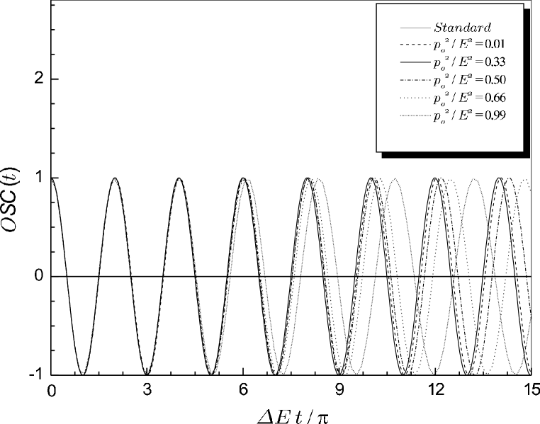
Figure 1: The time-behavior of $\mbox{\sc Osc}(t)$ compared with the standard plane wave oscillation given by $\cos{[\Delta E\,t]}$ for different propagation regimes. The additional phase $\Theta(t)$ changes the oscillating character after some time of propagation. The maximal deviation occurs for $\frac{p_{o}^{\mbox{\tiny$2$}}}{\bar{E}^{\mbox{\tiny$2$}}}\approx\frac{1}{3}$.

The oscillating function $\mbox{\sc Osc}(t)$ of the interference term $\mbox{\sc Sfo}(t)$ differs from the standard oscillating term, $\cos{[\Delta E\,t]}$, by the presence of the additional phase $\Theta(t)$ which is essentially a second order correction. The modifications introduced by the additional phase $\Theta(t)$ are discussed in Fig. 1 [11] where we have compared the time-behavior of $\mbox{\sc Osc}(t)$ to $\cos{[\Delta E\,t]}$ for different propagation regimes. The bound effective value assumed by $\Theta(t)$ is determined by the vanishing behavior of $\mbox{\sc Bnd}(t)$.

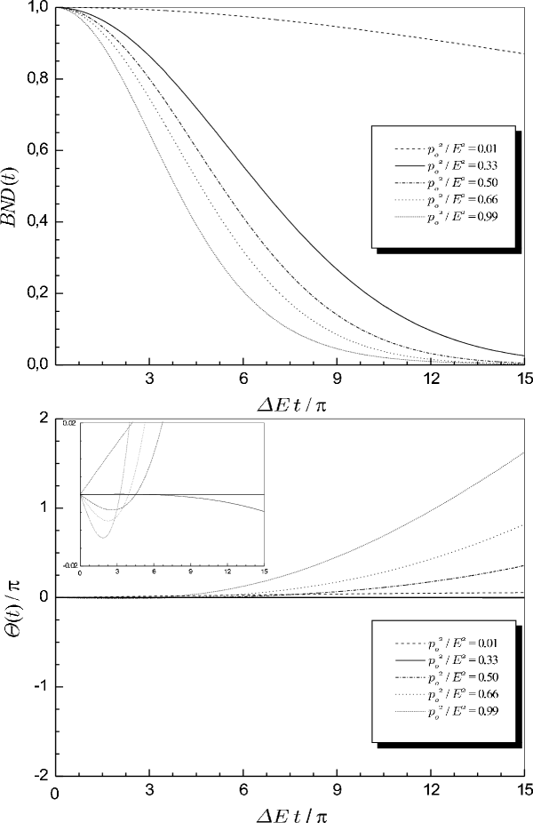
Figure 2: The time-behavior of the additional phase $\Theta(t)$. The values assumed by $\Theta(t)$ are effective while the interference term does not vanish. In the upper box we can observe the behavior of $\mbox{\sc Bnd}(t)$ which determines the limit values effectively assumed by $\Theta(t)$ for each propagation regime. For relativistic regimes with $\frac{p_{\mbox{\tiny$0$}}^{\mbox{\tiny$2$}}}{\bar{E}^{\mbox{\tiny$2$}}}>\frac{1}{3}$, the function $\Theta(t)$ rapidly reaches its lower limit as we can observe in the small box above. We have used $a\,\bar{E}=10$.

To illustrate this scalar flavor oscillation behavior, we plot both the curves representing $\mbox{\sc Bnd}(t)$ and $\Theta(t)$ in Fig. 2 [11]. We note the phase slowly changing in the NR regime. The modulus of the phase $|\Theta(t)|$ rapidly reaches its upper limit when $\frac{p_{\mbox{\tiny$0$}}^{\mbox{\tiny$2$}}}{\bar{E}^{\mbox{\tiny$2$}}}>\frac{1}{3}$ and, after a certain time, it continues to evolve approximately linearly in time. But, effectively, the oscillations rapidly vanishes. By superposing the effects of $\mbox{\sc Bnd}(t)$ in Fig. 2 and the oscillating character $\mbox{\sc Osc}(t)$ expressed in Fig. 1, we immediately obtain the flavor oscillation probability which is explicitly given by

$$P_{\mbox{\tiny$scalar$}}(\mbox{\boldmath$\nu_{\alpha}$}\rightarrow\mbox{\boldmath$\nu_{\beta}$};t)\approx\mbox{$\frac{\sin^{\mbox{\tiny$2$}}{[2\theta]}}{2}$}\left\{1-\left[1+\mbox{\sc Sp}^{\mbox{\tiny$2$}}(t)\right]^{-\frac{1}{4}}\right.\left.\exp{\left[-\frac{(\Delta\mbox{v}\,t)^{\mbox{\tiny$2$}}}{2a^{\mbox{\tiny$2$}}\left[1+\mbox{\sc Sp}^{\mbox{\tiny$2$}}(t)\right]}\right]}\cos{\left[\Delta E\,t+\Theta(t)\right]}\right\}.$$ (19)

Obviously, the larger is the value of $a\,\bar{E}$, the smaller are the wave packet effects. If it was sufficiently larger to not consider the second order corrections expressed in Eq. (9), we could compute the oscillation probability with the leading corrections due to the slippage effect,

$$P_{\mbox{\tiny$scalar$}}(\mbox{\boldmath$\nu_{\alpha}$}\rightarrow\mbox{\boldmath$\nu_{\beta}$};t)\approx\mbox{$\frac{\sin^{\mbox{\tiny$2$}}{[2\theta]}}{2}$}\left\{1-\exp{\left[-\frac{(\Delta\mbox{v}\,t)^{\mbox{\tiny$2$}}}{2\,a^{\mbox{\tiny$2$}}}\right]}\cos{[\Delta E\,t]}\right\}$$ (20)

which corresponds to the same result obtained by [7]. By assuming an UR propagation regime with $t\approx L$ and $E_{i}\sim p_{\mbox{\tiny$0$}}$, under minimal slippage conditions ($\Delta\mbox{v}\,L\ll a$), the above expression reproduces the standard plane wave result,

$$P_{\mbox{\tiny$scalar$}}(\mbox{\boldmath$\nu_{\alpha}$}\rightarrow\mbox{\boldmath$\nu_{\beta}$};L) \approx \frac{\sin^{\mbox{\tiny$2$}}{[2\theta]}}{2}\left\{1-\left[1-\frac{(\Delta\mbox{v}\,L)^{\mbox{\tiny$2$}}}{2\,a^{\mbox{\tiny$2$}}}\right]\cos{\left[\Delta E\,L\right]}\right\}$$ (21)

$$\approx \mbox{$\frac{\sin^{\mbox{\tiny$2$}}{[2\theta]}}{2}\left\{1-\cos{\left[\frac{\Delta m^{\mbox{\tiny$2$}}}{4p_{\mbox{\tiny$0$}}}\,L\right]}\right\}$},$$

$$= \mbox{$\sin^{\mbox{\tiny$2$}}[2\theta]\sin^{\mbox{\tiny$2$}}\left[\frac{\Delta m^{\mbox{\tiny$2$}}}{4p_{\mbox{\tiny$0$}}}\,L\right]$}.$$

since we have assumed $a\,\bar{E}\gg 1$.

III. Dirac Formalism

The results in the previous section have been obtained by considering scalar mass-eigenstates. Neutrinos are, however, fermions. The time evolution of a spin one-half particle must be described by the Dirac equation. To introduce the fermionic character in the study of quantum oscillation phenomena, we shall use the Dirac equation as the evolution equation for the mass-eigenstates. The Eq. (1) now becomes

$$\Psi(z,t) = \psi_{\mbox{\tiny$1$}}(z,t)\cos{\theta}\,\mbox{\boldmath$\nu_{\mbox{\tiny$1$}}$}+\psi_{\mbox{\tiny$2$}}(z,t)\sin{\theta}\,\mbox{\boldmath$\nu_{\mbox{\tiny$2$}}$}$$ (22)

$$= \left[\psi_{\mbox{\tiny$1$}}(z,t)\cos^{2}{\theta}+\psi_{\mbox{\tiny$2$}}(z,t)\sin^{2}{\theta}\right]\,\mbox{\boldmath$\nu_{\alpha}$}+\left[\psi_{\mbox{\tiny$1$}}(z,t)-\psi_{\mbox{\tiny$2$}}(z,t)\right]\cos{\theta}\sin{\theta}\,\mbox{\boldmath$\nu_{\beta}$}$$

$$= \psi_{\alpha}(z,t;\theta)\,\mbox{\boldmath$\nu_{\alpha}$}+\psi_{\beta}(z,t;\theta)\,\mbox{\boldmath$\nu_{\beta}$},$$

where $\psi_{i}(z,t)$ satisfies the Dirac equation for a mass $m_{i}$. The natural extension of Eq. (8) reads

$$\psi_{\alpha}(z,0,\theta)=\phi_{\alpha}(z,0,\theta)\,w$$ (23)

where $w$ is a constant spinor which satisfies the normalization condition $w^{\dagger}w=1$.

III.1. Dirac wave packets and the oscillation formula

To describe the time evolution of mass-eigenstate Dirac wave packets, we could be inclined to superpose only positive frequency solutions of the Dirac equation. It seems, at first glance, a reasonable choice. However, when the initial state has the form given in Eq. (23), it is necessary to superpose both positive and negative frequency solutions of Dirac equation. In order to clear up this point, let us express the flavor state $\psi_{\alpha}(z,t,\theta)$ in terms of

$$\psi_{i}(z,t) = \int_{{}_{-\infty}}^{{}^{+\infty}}\frac{dp_{\mbox{\tiny$z$}}}{2\pi}\exp{[ip_{\mbox{\tiny$z$}}z]}\sum_{i=1,2}\{b^{s}(p_{\mbox{\tiny$z$}},m_{\mbox{\tiny$i$}})\,u^{s}(p_{\mbox{\tiny$z$}},m_{\mbox{\tiny$i$}})\exp{[-iE(p_{\mbox{\tiny$z$}},m_{\mbox{\tiny$i$}})t]}$$ (24)

$$~{}~{}~{}~{}~{}~{}~{}~{}~{}~{}~{}~{}~{}~{}~{}~{}~{}~{}~{}~{}~{}~{}~{}~{}~{}~{}~{}~{}~{}~{}~{}~{}~{}~{}~{}~{}~{}+d^{s*}(\mbox{\tiny$-$}p_{\mbox{\tiny$z$}},m_{\mbox{\tiny$i$}})\,v^{s}(\mbox{\tiny$-$}p_{\mbox{\tiny$z$}},m_{\mbox{\tiny$i$}})\exp{[+iE(p_{\mbox{\tiny$z$}},m_{\mbox{\tiny$i$}})t]}\}.$$

At time $t=0$ the mass-eigenstate wave functions satisfy $\psi_{\mbox{\tiny$1$}}(z,0)=\psi_{\mbox{\tiny$2$}}(z,0)$ (this guarantees the instantaneous creation of a pure flavor-eigenstate $\nu_{\alpha}$ as we have appointed in section II). The Fourier transform of $\psi_{i}(z,0)$ is

$$\sum_{i=1,2}\left[b^{s}(p_{\mbox{\tiny$z$}},m_{\mbox{\tiny$i$}})\,u^{s}(p_{\mbox{\tiny$z$}},m_{\mbox{\tiny$i$}})+d^{s*}(\mbox{\tiny$-$}p_{\mbox{\tiny$z$}},m_{\mbox{\tiny$i$}})\,v^{s}(\mbox{\tiny$-$}p_{\mbox{\tiny$z$}},m_{\mbox{\tiny$i$}})\right].$$ (25)

By observing that the Fourier transform of $\phi_{\alpha}(z,0,\theta)$ is given by $\varphi(p_{\mbox{\tiny$z$}}-p_{\mbox{\tiny$0$}})$ (see Eq. (8)), we immediately obtain the Fourier transform of $\psi_{\alpha}(z,0,\theta)$,

$$\varphi(p_{\mbox{\tiny$z$}}-p_{\mbox{\tiny$0$}})w = \sum_{i=1,2}\left[b^{s}(p_{\mbox{\tiny$z$}},m_{\mbox{\tiny$i$}})\,u^{s}(p_{\mbox{\tiny$z$}},m_{\mbox{\tiny$i$}})+d^{s*}(\mbox{\tiny$-$}p_{\mbox{\tiny$z$}},m_{\mbox{\tiny$i$}})\,v^{s}(\mbox{\tiny$-$}p_{\mbox{\tiny$z$}},m_{\mbox{\tiny$i$}})\right].$$ (26)

Using the orthogonality properties of Dirac spinors, we find [14]

$$b^{s}(p_{\mbox{\tiny$z$}},m_{\mbox{\tiny$i$}}) = \varphi(p_{\mbox{\tiny$z$}}-p_{\mbox{\tiny$0$}})\,u^{s\dagger}(p_{\mbox{\tiny$z$}},m_{\mbox{\tiny$i$}})\,w,$$

$$d^{s*}(\mbox{\tiny$-$}p_{\mbox{\tiny$z$}},m_{\mbox{\tiny$i$}}) = \varphi(p_{\mbox{\tiny$z$}}-p_{\mbox{\tiny$0$}})\,v^{s\dagger}(\mbox{\tiny$-$}p_{\mbox{\tiny$z$}},m_{\mbox{\tiny$i$}})\,w.$$ (27)

These coefficients carry an important physical information. For any initial state which has the form given in Eq. (23), the negative frequency solution coefficient $d^{s*}(\mbox{\tiny$-$}p_{\mbox{\tiny$z$}},m_{\mbox{\tiny$i$}})$ necessarily provides a non-null contribution to the time evolving wave packet. This obliges us to take the complete set of Dirac equation solutions to construct the wave packet. Only if we consider a momentum distribution given by a delta function (plane wave limit) and suppose an initial spinor $w$ being a positive energy mass-eigenstate with momentum $p_{\mbox{\tiny$0$}}$, the contribution due to the negative frequency solutions $d^{s*}(\mbox{\tiny$-$}p_{\mbox{\tiny$z$}},m_{\mbox{\tiny$i$}})$ will be null.

Having introduced the Dirac wave packet prescription, we are now in a position to calculate the flavor conversion formula. The following calculations do not depend on the gamma matrix representation. By substituting the coefficients given by Eq. (27) in Eq. (24) and using the well-known spinor properties [14],

$$\sum_{i=1,2}u^{s}(p_{\mbox{\tiny$z$}},m_{\mbox{\tiny$i$}})\overline{u}^{s}(p_{\mbox{\tiny$z$}},m_{\mbox{\tiny$i$}})=\frac{\gamma^{0}E(p_{\mbox{\tiny$z$}},m_{\mbox{\tiny$i$}})-\gamma^{3}p_{\mbox{\tiny$z$}}+m_{i}}{2E(p_{\mbox{\tiny$z$}},m_{\mbox{\tiny$i$}})},$$

$$\sum_{i=1,2}v^{s}(\mbox{\tiny$-$}p_{\mbox{\tiny$z$}},m_{\mbox{\tiny$i$}})\overline{v}^{s}(\mbox{\tiny$-$}p_{\mbox{\tiny$z$}},m_{\mbox{\tiny$i$}})=\frac{\gamma^{0}E(p_{\mbox{\tiny$z$}},m_{\mbox{\tiny$i$}})+\gamma^{3}p_{\mbox{\tiny$z$}}-m_{i}}{2E(p_{\mbox{\tiny$z$}},m_{\mbox{\tiny$i$}})},$$ (28)

we obtain

$$\psi_{i}(z,t) = \int_{{}_{-\infty}}^{{}^{+\infty}}\frac{dp_{\mbox{\tiny$z$}}}{2\pi}\,\varphi(p_{\mbox{\tiny$z$}}-p_{\mbox{\tiny$0$}})\,\exp{[ip_{\mbox{\tiny$z$}}z]}\left\{\cos{[E(p_{\mbox{\tiny$z$}},m_{\mbox{\tiny$i$}})t]}-\frac{i\gamma^{0}\left(\gamma^{3}p_{\mbox{\tiny$z$}}+m_{i}\right)}{E(p_{\mbox{\tiny$z$}},m_{\mbox{\tiny$i$}})}\sin{[E(p_{\mbox{\tiny$z$}},m_{\mbox{\tiny$i$}})t]}\right\}\,w.~{}~{}~{}~{}~{}$$ (29)

By simple mathematical manipulations, the new interference oscillating term will be written as

$$\mbox{\sc Dfo}(t) = \int_{{}_{-\infty}}^{{}^{+\infty}}\frac{dp_{\mbox{\tiny$z$}}}{2\pi}\,\varphi^{2}(p_{\mbox{\tiny$z$}}-p_{\mbox{\tiny$0$}})\left\{\,\left[\,1-f(p_{\mbox{\tiny$z$}},m_{\mbox{\tiny$1$}},m_{\mbox{\tiny$2$}})\,\right]\,\cos[\epsilon_{\mbox{\tiny$-$}}(p_{\mbox{\tiny$z$}},m_{\mbox{\tiny$1$}},m_{\mbox{\tiny$2$}})\,t]\right.+$$ (30)

$$~{}~{}~{}~{}~{}~{}~{}~{}~{}~{}~{}~{}~{}~{}~{}~{}~{}~{}~{}~{}~{}~{}~{}~{}~{}~{}~{}~{}~{}~{}~{}~{}~{}~{}~{}~{}~{}~{}~{}~{}~{}~{}~{}~{}~{}~{}~{}~{}\left.f(p_{\mbox{\tiny$z$}},m_{\mbox{\tiny$1$}},m_{\mbox{\tiny$2$}})\,\cos[\epsilon_{\mbox{\tiny$+$}}(p_{\mbox{\tiny$z$}},m_{\mbox{\tiny$1$}},m_{\mbox{\tiny$2$}})\,t]\right\}$$

where

$$f(p_{\mbox{\tiny$z$}},m_{\mbox{\tiny$1$}},m_{\mbox{\tiny$2$}})=\frac{E(p_{\mbox{\tiny$z$}},m_{\mbox{\tiny$1$}})E(p_{\mbox{\tiny$z$}},m_{\mbox{\tiny$2$}})-p_{\mbox{\tiny$z$}}^{\mbox{\tiny$2$}}-m_{\mbox{\tiny$1$}}m_{\mbox{\tiny$2$}}}{2\,E(p_{\mbox{\tiny$z$}},m_{\mbox{\tiny$1$}})E(p_{\mbox{\tiny$z$}},m_{\mbox{\tiny$2$}})}~{}~{}~{}\mbox{and}~{}~{}~{}\epsilon_{\pm}(p_{\mbox{\tiny$z$}},m_{\mbox{\tiny$1$}},m_{\mbox{\tiny$2$}})=E(p_{\mbox{\tiny$z$}},m_{\mbox{\tiny$1$}})\pm E(p_{\mbox{\tiny$z$}},m_{\mbox{\tiny$2$}})~{}.$$

The time-independent term $f(p_{\mbox{\tiny$z$}},m_{\mbox{\tiny$1$}},m_{\mbox{\tiny$2$}})$ deserves some comments. It has a minimum at $p_{\mbox{\tiny$z$}}=0$ and two maxima at $p_{z}=\pm\sqrt{m_{\mbox{\tiny$1$}}m_{\mbox{\tiny$2$}}}$. It goes rapidly to zero when $p_{\mbox{\tiny$z$}}\gg m_{1,2}$ (ultra-relativistic limit) as well as when $p_{\mbox{\tiny$0$}}\ll m_{1,2}$ (non-relativistic limit). It means that when we consider a momentum distribution sharply peaked around $p_{\mbox{\tiny$0$}}\gg m_{1,2}$ or $p_{\mbox{\tiny$0$}}\ll m_{1,2}$ the corrections introduced by $f(p_{\mbox{\tiny$z$}},m_{\mbox{\tiny$1$}},m_{\mbox{\tiny$2$}})$ are negligible. The maximum value of $f(p_{\mbox{\tiny$z$}},m_{\mbox{\tiny$1$}},m_{\mbox{\tiny$2$}})$ is

$$f_{max}(p_{\mbox{\tiny$z$}},m_{\mbox{\tiny$1$}},m_{\mbox{\tiny$2$}})=\frac{1}{2}-\frac{\sqrt{m_{\mbox{\tiny$1$}}m_{\mbox{\tiny$2$}}}}{m_{\mbox{\tiny$1$}}+m_{\mbox{\tiny$2$}}}$$ (31)

which vanishes in the limit $m_{\mbox{\tiny$1$}}=m_{\mbox{\tiny$2$}}$. The effects introduced by $f(p_{\mbox{\tiny$z$}},m_{\mbox{\tiny$1$}},m_{\mbox{\tiny$2$}})$ are relevant only when $\Delta m\approx m_{\mbox{\tiny$1$}}\gg m_{\mbox{\tiny$2$}}$. Meanwhile, what is interesting about the result in Eq. (30) is that it was obtained without any assumption on the initial spinor $w$. Otherwise, the initial spinor carries some fundamental physical information about the created state. And this could be relevant in the study of chiral oscillations [17] where the initial state plays a fundamental role. In comparison with the standard treatment of neutrino oscillations done by using scalar wave packets, where the interference term $\mbox{\sc Sfo}(t)$ is given by Eq. (7) with $\Delta E(p_{\mbox{\tiny$z$}})\equiv\epsilon_{\mbox{\tiny$-$}}(p_{\mbox{\tiny$z$}},m_{\mbox{\tiny$1$}},m_{\mbox{\tiny$2$}})$, we note in $\mbox{\sc Dfo}(t)$ two additional terms. In the first one, the standard oscillating term $\cos{[\epsilon_{\mbox{\tiny$-$}}(p_{\mbox{\tiny$z$}},m_{\mbox{\tiny$1$}},m_{\mbox{\tiny$2$}})\,t]}$, which arises from the interference between mass-eigenstate components of equal sign frequencies, is multiplied by a new factor obtained by the products $u^{\dagger}(p_{\mbox{\tiny$z$}},m_{\mbox{\tiny$1$}})\,u(p_{\mbox{\tiny$z$}},m_{\mbox{\tiny$2$}})$, $v^{\dagger}(\mbox{\tiny$-$}p_{\mbox{\tiny$z$}},m_{\mbox{\tiny$1$}})\,v(\mbox{\tiny$-$}p_{\mbox{\tiny$z$}},m_{\mbox{\tiny$2$}})$ and h.c.. The second one is a new oscillating term, $\cos{[\epsilon_{\mbox{\tiny$+$}}(p_{\mbox{\tiny$z$}},m_{\mbox{\tiny$1$}},m_{\mbox{\tiny$2$}})\,t]}$, which comes from the interference between mass-eigenstate components of positive and negative frequencies. The factor multiplying such an additional oscillating term is obtained by the products $u^{\dagger}(p_{\mbox{\tiny$z$}},m_{\mbox{\tiny$1$}})\,v(\mbox{\tiny$-$}p_{\mbox{\tiny$z$}},m_{\mbox{\tiny$2$}})$, $v^{\dagger}(\mbox{\tiny$-$}p_{\mbox{\tiny$z$}},m_{\mbox{\tiny$1$}})\,u(p_{\mbox{\tiny$z$}},m_{\mbox{\tiny$2$}})$ and h.c.. The new oscillations have very high frequencies. Such a peculiar oscillating behavior is similar to the phenomenon referred to as Zitterbewegung. In atomic physics, the electron exhibits this violent quantum fluctuation in the position and becomes sensitive to an effective potential which explains the Darwin term in the hydrogen atom [18]. We shall see later that, at the instant of creation, such rapid oscillations introduce a small modification in the oscillation formula.

Returning to the starting point, if we had postulated a wave packet made up exclusively of positive frequency plane-wave solutions, the oscillation term $\cos{[\epsilon_{\mbox{\tiny$+$}}(p_{\mbox{\tiny$z$}},m_{\mbox{\tiny$1$}},m_{\mbox{\tiny$2$}})\,t]}$ would have vanished. It reinforces the argument that, in constructing Dirac wave packets, we cannot simply forget the contributions of negative frequency components.

III.2. First order modifications to the oscillation formula

A more satisfactory interpretation of the modifications introduced by the Dirac formalism is given when we explicitly calculate $\mbox{\sc Dfo}(t)$. By considering the energy $E(p_{\mbox{\tiny$z$}},m_{\mbox{\tiny$i$}})$ expansion up to the second order terms in Eq. (10), we include an analysis of spreading effects. In this preliminary study, we are, however, interested only to first order corrections. Thus, we approximate the frequency components by

$$E(p_{\mbox{\tiny$z$}},m_{\mbox{\tiny$i$}})\approx\,E_{\mbox{\tiny$i$}}\,+\mbox{v}_{\mbox{\tiny$i$}}\,\left(p_{\mbox{\tiny$z$}}-p_{\mbox{\tiny$0$}}\,\right)~{}.$$ (32)

As a consequence of this approximation, we get

$$f(p_{\mbox{\tiny$z$}},m_{\mbox{\tiny$1$}},m_{\mbox{\tiny$2$}}) \approx \mbox{$\frac{1}{2}$}\,\left\{1-\mbox{v}_{\mbox{\tiny$1$}}\mbox{v}_{\mbox{\tiny$2$}}\left(1+\frac{m_{\mbox{\tiny$1$}}m_{\mbox{\tiny$2$}}}{p_{\mbox{\tiny$0$}}^{\mbox{\tiny$2$}}}\right)+\mbox{v}_{\mbox{\tiny$1$}}\mbox{v}_{\mbox{\tiny$2$}}\,\left[\left(\mbox{v}_{\mbox{\tiny$1$}}^{\mbox{\tiny$2$}}+\mbox{v}_{\mbox{\tiny$2$}}^{\mbox{\tiny$2$}}\right)\left(1+\frac{m_{\mbox{\tiny$1$}}m_{\mbox{\tiny$2$}}}{p_{\mbox{\tiny$0$}}^{\mbox{\tiny$2$}}}\right)-2\right]\,\frac{p_{\mbox{\tiny$z$}}-p_{\mbox{\tiny$0$}}}{p_{\mbox{\tiny$0$}}}\,\right\}$$ (33)

and

$$\epsilon_{\mbox{\tiny$\pm$}}(p_{\mbox{\tiny$z$}},m_{\mbox{\tiny$1$}},m_{\mbox{\tiny$2$}}) \approx E_{\mbox{\tiny$1$}}\pm E_{\mbox{\tiny$2$}}+\left(\,\mbox{v}_{\mbox{\tiny$1$}}\pm\mbox{v}_{\mbox{\tiny$2$}}\,\right)\,\left(p_{\mbox{\tiny$z$}}-p_{\mbox{\tiny$0$}}\,\right)~{}.$$ (34)

For UR particles ($m_{\mbox{\tiny$i$}}\ll p_{\mbox{\tiny$0$}}$), we can also use the following expression for the central energy values ($E_{\mbox{\tiny$i$}}$) and the group velocities ($\mbox{v}_{\mbox{\tiny$i$}}$) of the mass-eigenstate wave packets,

$$E_{\mbox{\tiny$i$}}\approx\,p_{\mbox{\tiny$0$}}+\frac{m_{\mbox{\tiny$i$}}^{\mbox{\tiny$2$}}}{2\,p_{\mbox{\tiny$0$}}}~{}~{}~{}~{}~{}\mbox{and}~{}~{}~{}~{}~{}\mbox{v}_{\mbox{\tiny$i$}}\approx\,1-\frac{m_{\mbox{\tiny$i$}}^{\mbox{\tiny$2$}}}{2\,p_{\mbox{\tiny$0$}}^{\,\mbox{\tiny$2$}}}~{}.$$

This implies

$$f(p_{\mbox{\tiny$z$}},m_{\mbox{\tiny$1$}},m_{\mbox{\tiny$2$}}) \approx \left(\frac{\Delta m}{2\,p_{\mbox{\tiny$0$}}}\right)^{2}\,\left(\,1-2\,\,\frac{p_{\mbox{\tiny$z$}}-p_{\mbox{\tiny$0$}}}{p_{\mbox{\tiny$0$}}}\,\right)\,\,,$$

$$\epsilon_{\mbox{\tiny$+$}}(p_{\mbox{\tiny$z$}},m_{\mbox{\tiny$1$}},m_{\mbox{\tiny$2$}}) \approx 2\,p_{\mbox{\tiny$0$}}\,\left[\,1\,+\,\frac{m_{\mbox{\tiny$1$}}^{\mbox{\tiny$2$}}+m_{\mbox{\tiny$2$}}^{\mbox{\tiny$2$}}}{4\,p_{\mbox{\tiny$0$}}^{\,\mbox{\tiny$2$}}}\,+\,\frac{p_{\mbox{\tiny$z$}}-p_{\mbox{\tiny$0$}}}{p_{\mbox{\tiny$0$}}}\,\left(\,1-\frac{m_{\mbox{\tiny$1$}}^{\mbox{\tiny$2$}}+m_{\mbox{\tiny$2$}}^{\mbox{\tiny$2$}}}{4\,p_{\mbox{\tiny$0$}}^{\,\mbox{\tiny$2$}}}\,\right)\,\right]\,\,,$$

$$\epsilon_{\mbox{\tiny$-$}}(p_{\mbox{\tiny$z$}},m_{\mbox{\tiny$1$}},m_{\mbox{\tiny$2$}}) \approx \frac{\Delta m^{\mbox{\tiny$2$}}}{2\,p_{\mbox{\tiny$0$}}}\,\left[\,1-\,\frac{p_{\mbox{\tiny$z$}}-p_{\mbox{\tiny$0$}}}{p_{\mbox{\tiny$0$}}}\,\right]\,\,.$$

where $(\Delta m)^{\mbox{\tiny$2$}}=(m_{\mbox{\tiny$1$}}-m_{\mbox{\tiny$2$}})^{\mbox{\tiny$2$}}$ is different from $\Delta m^{\mbox{\tiny$2$}}=m_{\mbox{\tiny$1$}}^{\mbox{\tiny$2$}}-m_{\mbox{\tiny$2$}}^{\mbox{\tiny$2$}}$ which appears in the standard oscillation phase. Finally, by simple algebraic manipulations and after gaussian integrations, we find

$$\mbox{\sc Dfo}(t) \approx \exp{\left[-\left(\frac{\Delta m^{2}\,t}{2\sqrt{2}ap_{\mbox{\tiny$0$}}^{2}}\right)^{2}\right]}\left\{\left[1-\left(\frac{\Delta m}{2p_{\mbox{\tiny$0$}}}\right)^{2}\right]\cos{\left[\frac{\Delta m^{2}}{2p_{\mbox{\tiny$0$}}}t\right]}+\left(\frac{\Delta m}{2p_{\mbox{\tiny$0$}}}\right)^{2}\frac{\Delta m^{2}}{a^{2}p_{\mbox{\tiny$0$}}^{3}}t\sin{\left[\frac{\Delta m^{2}}{2p_{\mbox{\tiny$0$}}}t\right]}\right\}$$ (35)

$$+ \exp{\left[-\frac{t^{2}}{2a^{2}}\left(2-\frac{m_{\mbox{\tiny$1$}}^{2}+m_{\mbox{\tiny$2$}}^{2}}{2p_{\mbox{\tiny$0$}}^{2}}\right)^{2}\right]}\left(\frac{\Delta m}{2p_{\mbox{\tiny$0$}}}\right)^{2}\left\{\cos{\left[p_{\mbox{\tiny$0$}}t\left(2+\frac{m_{\mbox{\tiny$1$}}^{2}+m_{\mbox{\tiny$2$}}^{2}}{2p_{\mbox{\tiny$0$}}^{2}}\right)\right]}\right.$$

$$\mbox{$\left.~{}~{}~{}~{}~{}~{}~{}~{}~{}~{}~{}~{}~{}~{}~{}~{}~{}~{}~{}~{}~{}~{}~{}~{}~{}~{}~{}~{}~{}~{}~{}~{}~{}~{}~{}+\frac{2p_{\mbox{\tiny$0$}}t}{(ap_{\mbox{\tiny$0$}})^{2}}\left(2-\frac{m_{\mbox{\tiny$1$}}^{2}+m_{\mbox{\tiny$2$}}^{2}}{2p_{\mbox{\tiny$0$}}^{2}}\right)\sin{\left[p_{\mbox{\tiny$0$}}t\left(2+\frac{m_{\mbox{\tiny$1$}}^{2}+m_{\mbox{\tiny$2$}}^{2}}{2p_{\mbox{\tiny$0$}}^{2}}\right)\right]}\right\}$}.$$

As we have already noticed, the oscillating functions going with the second exponential function in Eq. (35) arise from the interference between positive and negative frequency solutions of the Dirac equation. It produces very high frequency oscillations which is similar to the quoted phenomenon of Zitterbewegung [18]. The oscillation length which characterizes the very high frequency oscillations is given by $L^{\tiny VHF}_{0sc}\approx\frac{2\pi}{p_{\mbox{\tiny$0$}}}$. Obviously, $L^{\tiny VHF}_{0sc}$ is much smaller than the standard oscillation length given by $L^{Std}_{0sc}=\frac{4\pi p_{\mbox{\tiny$0$}}}{\Delta m^{2}}$. It means that the propagating particle exhibits a violent quantum fluctuation of its flavor quantum number around a flavor average value which oscillates with $L^{Std}_{0sc}$. Meanwhile, except at times $t\sim 0$, it provides a practically null contribution to the oscillation probability. To explain such a statement, let us suppose that an experimental measurement takes place after a time $t\approx L$ for UR particles. The observability conditions impose that the propagation distance $L$ must be larger than the wave packet localization $a$. Since the (second) exponential function vanishes when $L\gg a$, for measurable distances, the effective flavor conversion formula will not contain such very high frequency oscillation terms, and can be written as

$$P_{\mbox{\tiny$Dirac$}}(\mbox{\boldmath$\nu_{\alpha}$}\rightarrow\mbox{\boldmath$\nu_{\beta}$};L) \approx \frac{\sin^{2}{[2\theta]}}{2}\left\{1-\exp{\left[-\left(\frac{\Delta m^{2}\,L}{2\sqrt{2}ap_{\mbox{\tiny$0$}}^{2}}\right)^{2}\right]}\left\{\left[1-\left(\frac{\Delta m}{2p_{\mbox{\tiny$0$}}}\right)^{2}\right]\cos{\left[\frac{\Delta m^{2}}{2p_{\mbox{\tiny$0$}}}L\right]}~{}~{}\right.\right.$$ (36)

$$\mbox{$\left.\left.~{}~{}~{}~{}~{}~{}~{}~{}~{}~{}~{}~{}~{}~{}~{}~{}~{}~{}~{}~{}~{}~{}~{}~{}~{}~{}~{}~{}~{}~{}~{}~{}~{}~{}~{}~{}~{}~{}~{}~{}~{}~{}~{}~{}~{}+\left(\frac{\Delta m}{2p_{\mbox{\tiny$0$}}}\right)^{2}\frac{\Delta m^{2}}{a^{2}p_{\mbox{\tiny$0$}}^{3}}L\sin{\left[\frac{\Delta m^{2}}{2p_{\mbox{\tiny$0$}}}L\right]}\right\}\right\}$}.$$

For distances which are restrict to the interval $a\ll L\ll a\frac{2\sqrt{2}p_{\mbox{\tiny$0$}}^{2}}{\Delta m^{2}}$ we observe the minimal slippage between the wave packets. In this case, we could suddenly approximate the oscillation probability to

$$P_{\mbox{\tiny$Dirac$}}(\mbox{\boldmath$\nu_{\alpha}$}\rightarrow\mbox{\boldmath$\nu_{\beta}$};L) \approx \frac{\sin^{2}{[2\theta]}}{2}\left\{1-\left[1-\left(\frac{\Delta m^{2}L}{2\sqrt{2}ap_{\mbox{\tiny$0$}}^{2}}\right)^{2}\right]\left[1-\left(\frac{\Delta m}{2p_{\mbox{\tiny$0$}}}\right)^{2}\right]\cos{\left[\frac{\Delta m^{2}}{2p_{\mbox{\tiny$0$}}}L\right]}\right\}$$ (37)

however, we reemphasize that it is not valid for $T\approx L\sim 0$ when the rapid oscillations are still relevant ($L<a$). By comparing the result of Eq. (37) with the scalar oscillation probability of Eq. (12), we notice a deviation of the order $\left(\frac{\Delta m}{2p_{\mbox{\tiny$0$}}}\right)^{2}$ that appears as an additional coefficient of the cosine function. It is not relevant in the UR limit as we have noticed after studying the function $f(p_{\mbox{\tiny$z$}},m_{\mbox{\tiny$1$}},m_{\mbox{\tiny$2$}})$.

III.3. A brief extension to quantum field treatment

Now we try to establish a tenuous correspondence between our results and the quantum field theory (QFT) treatment. It was extensively demonstrated in the literature [6, 16, 5] that the oscillating particle cannot be treated in isolation. The oscillation process must be considered globally: the oscillating states become intermediate states, not directly observed, which propagate between a source and a detector. This idea can be implemented in QFT when the intermediate oscillating states are represented by internal lines of Feynman diagrams and the interacting particles at source/detector are described by external wave packets [16, 1]. In this context, let us consider the weak flavor-changing processes occurring through the intermediate propagation of a neutrino,

$$p_{I}\rightarrow p_{F}+\alpha+\nu_{\alpha}~{}~{}(oscillation)~{}~{}\nu_{\beta}+D_{I}\rightarrow\beta+D_{F}$$ (38)

where $p_{I}$ and $p_{F}$ ($D_{I}$ and $D_{F}$) are respectively the initial and final production (detection) particles. The amplitude for the process is represented by

$$\mathcal{A}=\mbox{$\left\langle p_{F},D_{F}\left|\mathbf{T}\left(\exp{\left[-i\,\int{dx^{\mbox{\tiny$4$}}\,\mathcal{H}_{I}}\right]}\right)-\mathbf{1}\right|p_{I},D_{I}\right\rangle$}$$ (39)

where $\mathcal{H}_{I}$ is the interaction Hamiltonian for the intermediate particle and $\mathbf{T}$ is the time ordering operator. After some mathematical manipulations [1], this amplitude can be represented by the integral

$$\mathcal{A} = \int{\frac{dE\,d^{\mbox{\tiny$3$}}\mathbf{p}}{(2\pi)^{\mbox{\tiny$4$}}}\,F(E,\mathbf{p})}\,G(E,\mathbf{p},t_{D},t_{P})\,\exp{[i\,\mathbf{p}\cdot(\mathbf{x}_{D}-\mathbf{x}_{P})]}$$ (40)

where the function $F(E,\mathbf{p})$ represents the overlap of the incoming and outgoing wave packets, both at the source and at the detector, and the Green function in the momentum space, $G(E,\mathbf{p},t_{D},t_{P})$, represents the fermion propagator which carries the information of the oscillation process. The overlap function is independent of production and detection times and positions ($t_{P}$, $t_{D}$, $\mathbf{x}_{P}$, $\mathbf{x}_{D})$ and depends on the the directions of incoming and outgoing momenta. In certain way, the physical conditions of source and detector, in terms of time and space intervals, are better defined in this framework than in the intermediate wave packet framework. Anyway, to understand the oscillation process we must turn back to the definition of mixing in quantum mechanics. It is similar in field theory, except that it applies to fields, not to physical states. This difference allows to bypass the problems arising in the definition of flavor and mass bases [1]. In one-dimensional spatial coordinates, the mixing is illustrated by the unitary transformation

$$\psi_{\sigma}(z,t;\theta)=\mathcal{G}^{\mbox{\tiny$-$}\mbox{\tiny$1$}}(\theta;t)\,\psi_{i}(z,t)\,\mathcal{G}(\theta;t)$$ (41)

as the result of the noncoincidence of the flavor basis ($\sigma=\,\alpha,\,\beta$) and the mass basis ($i=\,1,\,2$). The Eq. (41) gives the Eq. (22) when the generator of mixing transformations $\mathcal{G}(\theta;t)$ is given by

$$\mathcal{G}(\theta;t) = \exp[\theta\int\,dz\,\psi_{\mbox{\tiny$1$}}(z,t)\psi_{\mbox{\tiny$2$}}(z,t)-\psi_{\mbox{\tiny$2$}}(z,t)\psi_{\mbox{\tiny$1$}}(z,t)].$$ (42)

By taking the one-dimensional representation of Eq. (40), the propagator $G(E,p_{\mbox{\tiny$z$}},t_{D},t_{P})$ can also be written in the flavor basis as

$$G^{\alpha\beta}(\theta;E,p_{\mbox{\tiny$z$}},T) = \mathcal{G}^{\mbox{\tiny$-$}\mbox{\tiny$1$}}(\theta;t)\,G(E,p_{\mbox{\tiny$z$}},T)\,\mathcal{G}(\theta;t)=\mathcal{G}^{\mbox{\tiny$-$}\mbox{\tiny$1$}}(\theta;t)\,G(E,p_{\mbox{\tiny$z$}},t_{D},t_{P})\,\mathcal{G}(\theta;t)~{}~{}$$ (43)

with $T=t_{D}-t_{P}$.

In particular, by following the Blasone and Vitiello (BV) prescription [15, 19], the definition of a Fock space of weak eigenstates becomes possible and a nonperturbative flavor oscillation amplitude can be derived. In this case, the complete Lagrangian (density) is split in a propagation Lagrangian,

$$\mathcal{L}_{p}(z,t) = \bar{\psi}_{\mbox{\tiny$1$}}(z,t)\,\left(i\,\partial/\hskip 2.84544pt-m_{\mbox{\tiny$1$}}\right)\,\psi_{\mbox{\tiny$1$}}(z,t)+\bar{\psi}_{\mbox{\tiny$2$}}(z,t)\,\left(i\,\partial/\hskip 2.84544pt-m_{\mbox{\tiny$2$}}\right)\,\psi_{\mbox{\tiny$2$}}(z,t),$$ (44)

and an interaction Lagrangian

$$\mathcal{L}_{i}(z,t) = \bar{\psi}_{\alpha}(z,t;\theta)\,\left(i\,\partial/\hskip 2.84544pt-m_{\alpha}\right)\,\psi_{\alpha}(z,t;\theta)+\bar{\psi}_{\beta}(z,t;\theta)\,\left(i\,\partial/\hskip 2.84544pt-m_{\beta}\right)\,\psi_{\beta}(z,t;\theta)$$ (45)

$$~{}~{}~{}~{}~{}~{}~{}~{}~{}~{}~{}~{}~{}~{}~{}~{}~{}~{}~{}~{}~{}~{}~{}~{}~{}~{}~{}~{}~{}~{}~{}-m_{\alpha\beta}\,\left(\bar{\psi}_{\alpha}(z,t;\theta)\psi_{\beta}(z,t;\theta)+\bar{\psi}_{\beta}(z,t;\theta)\psi_{\alpha}(z,t;\theta)\right),$$

where

$$m_{\alpha(\beta)}=m_{\mbox{\tiny$1$}(\mbox{\tiny$2$})}\,\cos^{\mbox{\tiny$2$}}{\theta}+m_{\mbox{\tiny$2$}(\mbox{\tiny$1$})}\,\sin^{\mbox{\tiny$2$}}{\theta}~{}~{}~{}\mbox{and}~{}~{}~{}m_{\alpha\beta}=(m_{\mbox{\tiny$1$}}-m_{\mbox{\tiny$2$}})\,\cos{\theta}\sin{\theta}.$$

In general, the two subsets of the Lagrangian can be distinguished if there is a flavor transformation which is a symmetry of $\mathcal{L}_{i}(z,t)$ but not of $\mathcal{L}_{p}(z,t)$. Particle mixing occurs if the propagator built from $\mathcal{L}_{p}(z,t)$, and representing the creation of a particle of flavor $\alpha$ at point $z$ and the annihilation of a particle of flavor $\beta$ at point $z^{\prime}$, is not diagonal, i.e. not zero for $\beta=\alpha$. The free fields $\psi_{i}(z,t)$ can be quantized in the usual way by rewriting the momentum distributions $b^{s}(p_{\mbox{\tiny$z$}},m_{\mbox{\tiny$i$}})$ and $d^{s*}(\mbox{\tiny$-$}p_{\mbox{\tiny$z$}},m_{\mbox{\tiny$i$}})$ in Eq. (24) as creation and annihilation operators ${\sc B}^{s}(p_{\mbox{\tiny$z$}},m_{\mbox{\tiny$i$}})$ and ${\sc D}^{s\dagger}(\mbox{\tiny$-$}p_{\mbox{\tiny$z$}},m_{\mbox{\tiny$i$}})$. The interacting fields are then given by

$$\psi_{\sigma}(z,t) = \mbox{$\int_{{}_{\mbox{\tiny$-\infty$}}}^{{}^{\mbox{\tiny$+\infty$}}}\frac{dp_{\mbox{\tiny$z$}}}{2\pi}\exp{[ip_{\mbox{\tiny$z$}}z]}$}\sum_{i=1,2}\{{\sc B}^{s}_{\sigma}(p_{\mbox{\tiny$z$}};t)\,u^{s}_{\sigma}(p_{\mbox{\tiny$z$}};t)+{\sc D}^{s*}_{\sigma}(\mbox{\tiny$-$}p_{\mbox{\tiny$z$}};t)\,v^{s}_{\sigma}(\mbox{\tiny$-$}p_{\mbox{\tiny$z$}};t)\}$$ (46)

where the new flavor creation and annihilation operators which satisfy canonical anticommutation relations are defined by means of Bogoliubov transformations [19] as

$${\sc B}^{s}_{\sigma}(p_{\mbox{\tiny$z$}};t)=\mathcal{G}^{\mbox{\tiny$-$}\mbox{\tiny$1$}}(\theta;t)\,{\sc B}^{s}(p_{\mbox{\tiny$z$}},m_{\mbox{\tiny$i$}})\,\mathcal{G}(\theta;t)~{}~{}~{}\mbox{and}~{}~{}~{}{\sc D}^{s}_{\sigma}(\mbox{\tiny$-$}p_{\mbox{\tiny$z$}};t)=\mathcal{G}^{\mbox{\tiny$-$}\mbox{\tiny$1$}}(\theta;t)\,{\sc D}^{s}(\mbox{\tiny$-$}p_{\mbox{\tiny$z$}},m_{\mbox{\tiny$i$}})\,\mathcal{G}(\theta;t).$$

By following the BV prescription [15], which takes into account the above definitions, it was demonstrated [20] that the flavor conversion formula can be written as

$$P(\mbox{\boldmath$\nu_{\alpha}$}\rightarrow\mbox{\boldmath$\nu_{\beta}$};t) = \left|\left\{{\sc B}^{s}_{\beta}(p_{\mbox{\tiny$0$}};t),\,{\sc B}^{s}_{\alpha}(p_{\mbox{\tiny$0$}};t)\right\}\right|^{\mbox{\tiny$2$}}+\left|\left\{{\sc D}^{s}_{\beta}(\mbox{\tiny$-$}p_{\mbox{\tiny$0$}};t),\,{\sc B}^{s}_{\alpha}(p_{\mbox{\tiny$0$}};t)\right\}\right|^{\mbox{\tiny$2$}}$$ (47)

which is calculated without considering the localization conditions imposed by wave packets, i. e. by assuming that $p_{\mbox{\tiny$z$}}\approx p_{\mbox{\tiny$0$}}$. When the explicit form of the flavor annihilation and creation operators are substituted in Eq. (47), it was also demonstrated [19] that the flavor oscillation formula becomes

$$P(\mbox{\boldmath$\nu_{\alpha}$}\rightarrow\mbox{\boldmath$\nu_{\beta}$};t) = \mbox{$\frac{\sin^{\mbox{\tiny$2$}}{[2\theta]}}{2}$}\left\{\left[1-f(p_{\mbox{\tiny$0$}},m_{\mbox{\tiny$1$}},m_{\mbox{\tiny$2$}})\,\right]\,\cos[\epsilon_{\mbox{\tiny$-$}}(p_{\mbox{\tiny$0$}},m_{\mbox{\tiny$1$}},m_{\mbox{\tiny$2$}})\,t]\right.$$ (48)

$$\left.~{}~{}~{}~{}~{}~{}~{}~{}~{}~{}~{}~{}~{}~{}~{}~{}~{}~{}~{}~{}~{}~{}~{}+f(p_{\mbox{\tiny$0$}},m_{\mbox{\tiny$1$}},m_{\mbox{\tiny$2$}})\,\cos[\epsilon_{\mbox{\tiny$+$}}(p_{\mbox{\tiny$0$}},m_{\mbox{\tiny$1$}},m_{\mbox{\tiny$2$}})\,t]\right\}$$

$$\approx \sin^{\mbox{\tiny$2$}}{[2\theta]}\left\{\left[1-\left(\frac{\Delta m}{2p_{\mbox{\tiny$0$}}}\right)^{\mbox{\tiny$2$}}\right]\sin^{\mbox{\tiny$2$}}{\left[\frac{\Delta m^{\mbox{\tiny$2$}}}{4p_{\mbox{\tiny$0$}}}t\right]}+\left(\frac{\Delta m}{2p_{\mbox{\tiny$0$}}}\right)^{\mbox{\tiny$2$}}\sin^{\mbox{\tiny$2$}}{\left[p_{\mbox{\tiny$0$}}t\left(1+\frac{m_{\mbox{\tiny$1$}}^{\mbox{\tiny$2$}}+m_{\mbox{\tiny$2$}}^{\mbox{\tiny$2$}}}{4p_{\mbox{\tiny$0$}}^{\mbox{\tiny$2$}}}\right)\right]}\right\}~{}~{}$$

where the last approximation takes place in the relativistic limit $p_{\mbox{\tiny$0$}}\gg\sqrt{m_{\mbox{\tiny$1$}}m_{\mbox{\tiny$2$}}}$. After some simple mathematical manipulations, the Eq. (48) gives exactly the oscillation probability $P_{\mbox{\tiny$Dirac$}}(\mbox{\boldmath$\nu_{\alpha}$}\rightarrow\mbox{\boldmath$\nu_{\beta}$};L)$ calculated from Eq. (35) when it is assumed that the wave packet width $a$ tends to infinity and $t\approx L$.

This new oscillation formula tends to the standard one (21) in the UR limit. If the mass eigenstates were nearly degenerate, we could have focused on the case of a nonrelativistic oscillating particle having very distinct mass eigenstates. Under these conditions, the quantum theory of measurement says that interference vanishes. Therefore, as we have already appointed, the effects are, under realistic conditions, far from observable. Besides, in spite of working on a QFT framework, the lack of observability conditions must be overcome by implementing external wave packets, i. e. by calculating the explicit form of Eq. (40) for fermions. Such a procedure was applied by Beuthe for scalar particles [1] and, in a very particular analysis, with basis on the BV calculations and on our intermediate wave packet results, it could be extended to the fermionic case.

IV. Flavor and Chiral Oscillations

In treating the time evolution of the spinorial mass-eigenstate wave packets in the previous section, we have overlooked an important feature. We have completely disregarded the chiral nature of charged weak currents and the time evolution of the chiral operator. In the following, we aim to investigate if (and eventually how) the flavor oscillation formula could be modified by this additional effect.

It is well known that from the Heisenberg equation, we can immediately determine whether or not a given observable is a constant of the motion. If neutrinos have mass, the operator $\gamma^{\mbox{\tiny$5$}}$ does not commute with the mass-eigenstate Hamiltonians. This means that for massive neutrinos chirality is not a constant of the motion. Observing that neutrinos with positive chirality are decoupled from charged weak currents, this additional effect cannot be ignored. We have already seen that localized states contains, in general, plane-wave components of negative and positive frequencies. As an immediate consequence of this, the interference between positive and negative frequencies, responsible for the additional oscillatory term in $\mbox{\sc Dfo}(t)$, will also imply an oscillation in the average of chirality. Thus, the use of Dirac equation as evolution equation for neutrino mass-eigenstate wave packets leads to an oscillation formula containing both “flavor-appearance” (neutrinos of a flavor not present in the original source) and “chiral-disappearance” (neutrinos of wrong chirality) probabilities.

We obtain the Dirac flavor and chiral oscillation probability formula in the same way as we have obtained the Eq. (36). By assuming that the normalizable mass-eigenstate wave functions $\psi_{\mbox{\tiny$1$},\mbox{\tiny$2$}}(z,t)$ are created at time $t=0$ as a $-1$ chiral eigenstate, we can write

$$Re\left\{\int_{{}_{-\infty}}^{{}^{+\infty}}dz\,\psi^{\dagger}_{\mbox{\tiny$i$}}(z,t)\,\gamma^{\mbox{\tiny$5$}}\,\psi_{\mbox{\tiny$j$}}(z,t)\right\}=\int_{{}_{-\infty}}^{{}^{+\infty}}\frac{dp_{\mbox{\tiny$z$}}}{2\pi}\,\varphi^{2}(p_{\mbox{\tiny$z$}}-p_{\mbox{\tiny$0$}})$$ (49)

$$~{}~{}~{}~{}~{}~{}~{}~{}\times\left\{\,\left[\,1-f(p_{\mbox{\tiny$z$}},m_{\mbox{\tiny$i$}},m_{\mbox{\tiny$i$}})-\,\frac{m_{\mbox{\tiny$i$}}m_{\mbox{\tiny$i$}}}{E(p_{\mbox{\tiny$z$}},m_{\mbox{\tiny$i$}})E(p_{\mbox{\tiny$z$}},m_{\mbox{\tiny$i$}})}\,\right]\,\cos[\epsilon_{\mbox{\tiny$-$}}(p_{\mbox{\tiny$z$}},m_{\mbox{\tiny$i$}},m_{\mbox{\tiny$i$}})\,t]\right.$$

$$~{}~{}~{}~{}~{}~{}~{}~{}~{}~{}~{}~{}~{}~{}~{}~{}~{}~{}+\left.\left[\,f(p_{\mbox{\tiny$z$}},m_{\mbox{\tiny$i$}},m_{\mbox{\tiny$i$}})+\frac{m_{\mbox{\tiny$i$}}m_{\mbox{\tiny$i$}}}{E(p_{\mbox{\tiny$z$}},m_{\mbox{\tiny$i$}})E(p_{\mbox{\tiny$z$}},m_{\mbox{\tiny$i$}})}\,\right]\,\cos[\epsilon_{\mbox{\tiny$+$}}(p_{\mbox{\tiny$z$}},m_{\mbox{\tiny$i$}},m_{\mbox{\tiny$i$}})\,t]\right\}~{}~{}(\mbox{\footnotesize$i,j\,=\,1,2$})~{}.$$

From this integral, it is readily seen that an initial $-1$ chiral mass-eigenstate will evolve with time changing its chirality. Once we know the time evolution of the chiral operator, we are able to construct an effective oscillation probability which takes into account both flavor and chiral conversion effects, i.e.

$$P(\mbox{\boldmath$\nu_{\alpha,\mbox{\tiny$L$}}$}\rightarrow\mbox{\boldmath$\nu_{\beta,\mbox{\tiny$L$}}$};t) = \int_{{}_{-\infty}}^{{}^{+\infty}}dz\,|\psi_{\mbox{\tiny$\beta$},\mbox{\tiny$L$}}(z,t;\theta)|^{\mbox{\tiny$2$}}=\int_{{}_{-\infty}}^{{}^{+\infty}}dz\,\mbox{$\psi^{\prime}_{\mbox{\tiny$\beta$}}(z,t;\theta)\,\frac{1-\gamma^{\mbox{\tiny$5$}}}{2}\,\psi_{\mbox{\tiny$\beta$}}(z,t;\theta)$}$$ (50)

$$= \mbox{$\frac{\sin^{\mbox{\tiny$2$}}{[2\theta]}}{2}$}\,\left\{\,\frac{1}{2}\,\sum_{i=1}^{2}\,\left[\int_{{}_{-\infty}}^{{}^{+\infty}}dz\,|\psi_{\mbox{\tiny$i$},\mbox{\tiny$L$}}(z,t)|^{\mbox{\tiny$2$}}\right]-Re\left[\int_{{}_{-\infty}}^{{}^{+\infty}}dz\,\psi_{\mbox{\tiny$1$},\mbox{\tiny$L$}}^{\prime}(z,t)\,\psi_{\mbox{\tiny$2$},\mbox{\tiny$L$}}(z,t)\right]\right\}$$

$$= \mbox{$\frac{\sin^{\mbox{\tiny$2$}}{[2\theta]}}{2}$}\left[\mbox{\sc Dco}(t)-\mbox{\sc Dfco}(t)\right].$$

As done in the previous section, the terms $\mbox{\sc Dco}(t)$ and $\mbox{\sc Dfco}(t)$ can be rewritten by using a $p_{\mbox{\tiny$z$}}$-integration,

$$\mbox{\sc Dco}(t) = \frac{1}{2}\sum_{i=1}^{2}\,\int_{{}_{-\infty}}^{{}^{+\infty}}\frac{dp_{z}}{2\,\pi}\,\varphi^{\mbox{\tiny$2$}}(p_{\mbox{\tiny$z$}}-p_{\mbox{\tiny$0$}})\,\left\{\,1-c(p_{\mbox{\tiny$z$}},m_{\mbox{\tiny$i$}},m_{\mbox{\tiny$i$}})+c(p_{\mbox{\tiny$z$}},m_{\mbox{\tiny$i$}},m_{\mbox{\tiny$i$}})\,\cos[2\,E(p_{\mbox{\tiny$z$}},m_{\mbox{\tiny$i$}})\,t]\right\}$$ (51)

$$= 1-\frac{1}{2}\sum_{i=1}^{2}\,\int_{{}_{-\infty}}^{{}^{+\infty}}\frac{dp_{z}}{2\,\pi}\,\varphi^{\mbox{\tiny$2$}}(p_{\mbox{\tiny$z$}}-p_{\mbox{\tiny$0$}})\,\left\{\,\frac{m_{\mbox{\tiny$i$}}^{\mbox{\tiny$2$}}}{2\,E^{{}^{\,\mbox{\tiny$2$}}}(p_{\mbox{\tiny$z$}},m_{\mbox{\tiny$i$}})}-\frac{m_{\mbox{\tiny$i$}}^{\mbox{\tiny$2$}}}{2\,E^{{}^{\,\mbox{\tiny$2$}}}(p_{\mbox{\tiny$z$}},m_{\mbox{\tiny$i$}})}\cos[2\,E(p_{\mbox{\tiny$z$}},m_{\mbox{\tiny$i$}})\,t]\right\}$$

and

$$\mbox{\sc Dfco}(t) = \int_{{}_{-\infty}}^{{}^{+\infty}}\frac{dp_{z}}{2\,\pi}\,\varphi^{\mbox{\tiny$2$}}(p_{\mbox{\tiny$z$}}-p_{\mbox{\tiny$0$}})\,\left\{\,\left[\,1-c(p_{\mbox{\tiny$z$}},m_{\mbox{\tiny$1$}},m_{\mbox{\tiny$2$}})\,\right]\,\cos[\epsilon_{\mbox{\tiny$-$}}(p_{\mbox{\tiny$z$}},m_{\mbox{\tiny$1$}},m_{\mbox{\tiny$2$}})\,t]\right.$$ (52)

$$~{}~{}~{}~{}~{}~{}~{}~{}~{}~{}~{}~{}~{}~{}~{}~{}~{}~{}~{}~{}~{}~{}~{}~{}~{}~{}~{}~{}~{}~{}~{}~{}~{}~{}~{}~{}~{}~{}~{}~{}~{}+\left.c(p_{\mbox{\tiny$z$}},m_{\mbox{\tiny$1$}},m_{\mbox{\tiny$2$}})\,\cos[\epsilon_{\mbox{\tiny$+$}}(p_{\mbox{\tiny$z$}},m_{\mbox{\tiny$1$}},m_{\mbox{\tiny$2$}})\,t]\right\}~{},$$

where

$$c(p_{\mbox{\tiny$z$}},m_{\mbox{\tiny$i$}},m_{\mbox{\tiny$j$}})=f(p_{\mbox{\tiny$z$}},m_{\mbox{\tiny$i$}},m_{\mbox{\tiny$j$}})+\frac{m_{\mbox{\tiny$i$}}m_{\mbox{\tiny$j$}}}{2\,E(p_{\mbox{\tiny$z$}},m_{\mbox{\tiny$i$}})E(p_{\mbox{\tiny$z$}},m_{\mbox{\tiny$j$}})}~{}.$$

The functions $c(p_{\mbox{\tiny$z$}},m_{\mbox{\tiny$i$}},m_{\mbox{\tiny$j$}})$ have a common maximum at $p_{\mbox{\tiny$z$}}=0$ which, contrary to what happened for $f(p_{\mbox{\tiny$z$}},m_{\mbox{\tiny$1$}},m_{\mbox{\tiny$2$}})$, do not depend on the mass values,

$$c_{\mbox{\tiny max}}(0,m_{\mbox{\tiny$i$}},m_{\mbox{\tiny$j$}})=\mbox{$\frac{1}{2}$}\,\,,$$

and, following the same asymptotic behavior of $f(p_{\mbox{\tiny$z$}},m_{\mbox{\tiny$1$}},m_{\mbox{\tiny$2$}})$, go rapidly to zero for $p_{\mbox{\tiny$z$}}\gg m_{\mbox{\tiny$1$},\mbox{\tiny$2$}}$. As a consequence of the first order approximation (32), we get

$$c(p_{\mbox{\tiny$z$}},m_{\mbox{\tiny$i$}},m_{\mbox{\tiny$j$}}) \approx \mbox{$\frac{1}{2}$}\,\left[1-\mbox{v}_{\mbox{\tiny$i$}}\mbox{v}_{\mbox{\tiny$j$}}+\mbox{v}_{\mbox{\tiny$i$}}\mbox{v}_{\mbox{\tiny$j$}}\,\left(\mbox{v}_{\mbox{\tiny$i$}}^{\mbox{\tiny$2$}}+\mbox{v}_{\mbox{\tiny$j$}}^{\mbox{\tiny$2$}}-2\right)\,\frac{p_{\mbox{\tiny$z$}}-p_{\mbox{\tiny$0$}}}{p_{\mbox{\tiny$0$}}}\,\right].$$

which gives

$$c(p_{\mbox{\tiny$z$}},m_{\mbox{\tiny$1$}},m_{\mbox{\tiny$2$}}) \approx \frac{m_{\mbox{\tiny$1$}}^{\mbox{\tiny$2$}}+m_{\mbox{\tiny$2$}}^{\mbox{\tiny$2$}}}{4\,p_{\mbox{\tiny$0$}}^{\,\mbox{\tiny$2$}}}\,\left(\,1-2\,\,\frac{p_{\mbox{\tiny$z$}}-p_{\mbox{\tiny$0$}}}{p_{\mbox{\tiny$0$}}}\,\right)$$

in the UR approximation. By substituting $c(p_{\mbox{\tiny$z$}},m_{\mbox{\tiny$i$}},m_{\mbox{\tiny$j$}})$ in the above integrations (51-52) and after some algebraic manipulations, we explicitly calculate the terms $\mbox{\sc Dco}(t)$ and $\mbox{\sc Dfco}(t)$,

$$\mbox{\sc Dco}(t) \approx 1-\frac{m_{\mbox{\tiny$1$}}^{\mbox{\tiny$2$}}}{4\,p_{\mbox{\tiny$0$}}^{\,\mbox{\tiny$2$}}}+\exp\left[-\left(\,\frac{2\,p_{\mbox{\tiny$0$}}^{\,\mbox{\tiny$2$}}-m_{\mbox{\tiny$1$}}^{\mbox{\tiny$2$}}}{\sqrt{2}\,a\,p_{\mbox{\tiny$0$}}^{\,\mbox{\tiny$2$}}}\,t\right)^{\mbox{\tiny$2$}}\,\right]\,\frac{m_{\mbox{\tiny$1$}}^{\mbox{\tiny$2$}}}{4\,p_{\mbox{\tiny$0$}}^{\,\mbox{\tiny$2$}}}\,$$ (53)

$$\left.\times\left\{\cos\left[\frac{2\,p_{\mbox{\tiny$0$}}^{\,\mbox{\tiny$2$}}+m_{\mbox{\tiny$1$}}^{\mbox{\tiny$2$}}}{p_{\mbox{\tiny$0$}}}\,t\right]+\frac{4\,p_{\mbox{\tiny$0$}}^{\,\mbox{\tiny$2$}}-2\,m_{\mbox{\tiny$1$}}^{\mbox{\tiny$2$}}}{a^{\mbox{\tiny$2$}}p_{\mbox{\tiny$0$}}^{\,\mbox{\tiny$3$}}}\,t\,\sin\left[\frac{2\,p_{\mbox{\tiny$0$}}^{\,\mbox{\tiny$2$}}+m_{\mbox{\tiny$1$}}^{\mbox{\tiny$2$}}}{p_{\mbox{\tiny$0$}}}\,t\right]\,\right\}\,\right\}\,$$

$$-\frac{m_{\mbox{\tiny$2$}}^{\mbox{\tiny$2$}}}{4\,p_{\mbox{\tiny$0$}}^{\,\mbox{\tiny$2$}}}+\exp\left[-\left(\,\frac{2\,p_{\mbox{\tiny$0$}}^{\,\mbox{\tiny$2$}}-m_{\mbox{\tiny$2$}}^{\mbox{\tiny$2$}}}{\sqrt{2}\,a\,p_{\mbox{\tiny$0$}}^{\,\mbox{\tiny$2$}}}\,t\right)^{\mbox{\tiny$2$}}\,\right]\,\frac{m_{\mbox{\tiny$2$}}^{\mbox{\tiny$2$}}}{4\,p_{\mbox{\tiny$0$}}^{\,\mbox{\tiny$2$}}}\,$$

$$\mbox{$\times\left.\left\{\,\cos\left[\frac{2\,p_{\mbox{\tiny$0$}}^{\,\mbox{\tiny$2$}}+m_{\mbox{\tiny$2$}}^{\mbox{\tiny$2$}}}{p_{\mbox{\tiny$0$}}}\,t\right]+\frac{4\,p_{\mbox{\tiny$0$}}^{\,\mbox{\tiny$2$}}-2\,m_{\mbox{\tiny$2$}}^{\mbox{\tiny$2$}}}{a^{\mbox{\tiny$2$}}p_{\mbox{\tiny$0$}}^{\,\mbox{\tiny$3$}}}\,t\,\sin\left[\frac{2\,p_{\mbox{\tiny$0$}}^{\,\mbox{\tiny$2$}}+m_{\mbox{\tiny$2$}}^{\mbox{\tiny$2$}}}{p_{\mbox{\tiny$0$}}}\,t\right]\,\right\}\,\right\}\,\,$},$$

$$\mbox{\sc Dfco}(t) \approx \exp\left[-\left(\,\frac{\Delta m^{\mbox{\tiny$2$}}}{2\sqrt{2}\,a\,p_{\mbox{\tiny$0$}}^{\,\mbox{\tiny$2$}}}\,t\right)^{\mbox{\tiny$2$}}\right]\,$$ (54)

$$\times\left\{\,\,\left[1-\,\frac{m_{\mbox{\tiny$1$}}^{\mbox{\tiny$2$}}+m_{\mbox{\tiny$2$}}^{\mbox{\tiny$2$}}}{4\,p_{\mbox{\tiny$0$}}^{\,\mbox{\tiny$2$}}}\,\right]\,\cos\left[\frac{\Delta m^{\mbox{\tiny$2$}}}{2\,p_{\mbox{\tiny$0$}}}\,t\right]+\frac{m_{\mbox{\tiny$1$}}^{\mbox{\tiny$2$}}+m_{\mbox{\tiny$2$}}^{\mbox{\tiny$2$}}}{4\,p_{\mbox{\tiny$0$}}^{\,\mbox{\tiny$2$}}}\,\frac{\Delta m^{\mbox{\tiny$2$}}}{a^{\mbox{\tiny$2$}}p_{\mbox{\tiny$0$}}^{\,\mbox{\tiny$3$}}}\,\,t\,\sin\left[\frac{\Delta m^{\mbox{\tiny$2$}}}{2\,p_{\mbox{\tiny$0$}}}\,t\right]\,\right\}$$

$$+\exp\left[-\left(\,\frac{4\,p_{\mbox{\tiny$0$}}^{\,\mbox{\tiny$2$}}-m_{\mbox{\tiny$1$}}^{\mbox{\tiny$2$}}-m_{\mbox{\tiny$2$}}^{\mbox{\tiny$2$}}}{2\sqrt{2}\,a\,p_{\mbox{\tiny$0$}}^{\,\mbox{\tiny$2$}}}\,t\right)^{\mbox{\tiny$2$}}\,\right]\,\frac{m_{\mbox{\tiny$1$}}^{\mbox{\tiny$2$}}+m_{\mbox{\tiny$2$}}^{\mbox{\tiny$2$}}}{4\,p_{\mbox{\tiny$0$}}^{\,\mbox{\tiny$2$}}}\,$$

$$\mbox{$\left\{\,\times\cos\left[\frac{4\,p_{\mbox{\tiny$0$}}^{\,\mbox{\tiny$2$}}+m_{\mbox{\tiny$1$}}^{\mbox{\tiny$2$}}+m_{\mbox{\tiny$2$}}^{\mbox{\tiny$2$}}}{2\,p_{\mbox{\tiny$0$}}}\,t\right]+\frac{4\,p_{\mbox{\tiny$0$}}^{\,\mbox{\tiny$2$}}-m_{\mbox{\tiny$1$}}^{\mbox{\tiny$2$}}-m_{\mbox{\tiny$2$}}^{\mbox{\tiny$2$}}}{a^{\mbox{\tiny$2$}}p_{\mbox{\tiny$0$}}^{\,\mbox{\tiny$3$}}}\,t\,\sin\left[\frac{4\,p_{\mbox{\tiny$0$}}^{\,\mbox{\tiny$2$}}+m_{\mbox{\tiny$1$}}^{\mbox{\tiny$2$}}+m_{\mbox{\tiny$2$}}^{\mbox{\tiny$2$}}}{2\,p_{\mbox{\tiny$0$}}}\,t\right]\,\right\}\,\,$}.$$

Again, in the hypothesis of minimal slippage between the mass-eigenstate wave packets ($\Delta vL\ll a$), and for long distance between source and detector ($L\gg a$),i.e.

$$1\,\ll\frac{L}{a}\ll\frac{p_{\mbox{\tiny$0$}}^{\,\mbox{\tiny$2$}}}{\Delta\,m^{\mbox{\tiny$2$}}}\,,\,$$

the standard flavor oscillation probability is reproduced. In fact,

$$P\left(\boldsymbol{\nu_{\mbox{\tiny$\alpha$},\mbox{\tiny$L$}}}\to\boldsymbol{\nu_{\mbox{\tiny$\beta$},\mbox{\tiny$L$}}};\,L\right) \approx \frac{\sin^{\mbox{\tiny$2$}}{[2\theta]}}{2} \left[1-\,\frac{m_{\mbox{\tiny$1$}}^{\mbox{\tiny$2$}}+m_{\mbox{\tiny$2$}}^{\mbox{\tiny$2$}}}{4\,p_{\mbox{\tiny$0$}}^{\,\mbox{\tiny$2$}}}\,\right]\left\{\,1-\left[1-\left(\,\frac{\Delta m^{\mbox{\tiny$2$}}}{2\sqrt{2}\,a\,p_{\mbox{\tiny$0$}}^{\,\mbox{\tiny$2$}}}\,L\right)^{\mbox{\tiny$2$}}\right]\,\cos\left[\frac{\Delta m^{\mbox{\tiny$2$}}}{2\,p_{\mbox{\tiny$0$}}}\,L\right]\,\right\}$$ (55)

$$\approx \frac{\sin^{\mbox{\tiny$2$}}{[2\theta]}}{2} \left\{\,1-\cos\left[\frac{\Delta m^{\mbox{\tiny$2$}}}{2\,p_{\mbox{\tiny$0$}}}\,L\right]\,\right\}$$

$$= \sin^{\mbox{\tiny$2$}}[2\theta]\,\,\,\mbox{$\sin^{2}\left[\frac{\Delta m^{2}}{4p_{\mbox{\tiny$0$}}}\,L\right]$}~{}.$$

V. Conclusions

In order to quantify some subtle changes which appear in the standard flavor oscillation probability [9] due to chiral oscillations coupled to the flavor conversion mechanism of free propagating wave packets, we have reported about some recent results on the study of flavor oscillation with Dirac wave packets [11]. By taking into account the spinorial form of neutrino wave functions and imposing an initial constraint where a pure flavor-eigenstate is created at $t=0$, for a constant spinor $w$, it is possible to calculate the contribution of positive and negative frequency solutions of the Dirac equation to the wave packet propagation and, finally, to obtain the oscillation probability. Particularly, we have noticed a term of very high oscillation frequency depending on the sum of energies in the new oscillation probability formula. In addition, the spinorial form of the wave functions and their chiral oscillating character subtly modify the coefficients of the oscillating terms in this flavor conversion formula. To describe the time evolution of the mass-eigenstates, we have assumed an initial gaussian localization and performed integrations by considering a strictly peaked momentum distribution. Under the particular assumption of UR particles, we have been able to obtain an analytic expression for the coupled chiral and flavor conversion formula. In case of Dirac wave packets, these modifications introduce correction factors which are negligible in the UR limit. We have confirmed that the fermionic character of the particles modify the standard oscillation probability which is previously obtained by implicitly assuming a scalar nature of the mass-eigenstates.

However, we know the necessity of a more sophisticated approach is understood. It involves a field-theoretical treatment. Derivations of the oscillation formula resorting to field-theoretical methods are not very popular. They are thought to be very complicated and the existing quantum field computations of the oscillation formula do not agree in all respects [1]. The Blasone and Vitiello (BV) model [15, 2] to neutrino/particle mixing and oscillations seems to be the most distinguished trying to this aim. They have attempt to define a Fock space of weak eigenstates and to derive a nonperturbative oscillation formula. Flavor creation and annihilation operators, satisfying canonical (anti)comutation relations, are defined by means of Bogoliubov transformations. As a result, new oscillation formulas are obtained for fermions and bosons, with the oscillation frequency depending not only on the difference but also on the sum of the energies of the different mass-eigenstates. Meanwhile, the prescription of oscillating neutrinos as Dirac spinors was not yet completely and accurately described in a quantum field formalism. With Dirac wave packets, the flavor conversion formula can be reproduced [13] with the same mathematical structure as those obtained in the BV model [15, 2]. Moreover each new effect present in the oscillation formula can be separately quantified.

In fact, the quantum-mechanical treatment which associates Dirac wave packets with the propagating mass eigenstates is rich in physical insights which were extensively studied in this paper. Besides the review of analytical calculations done with gaussian wave packets for scalar [11] and fermionic [13] particles, the main conceptual aspect arising from the formalism with Dirac wave packets leads to the study of chiral oscillations. In the standard model flavor-changing interactions, neutrinos with positive chirality are decoupled from the neutrino absorbing charged weak currents [17]. A state with left-handed helicity can be approximated by a state with negative chirality in the UR limit. Once we have assumed the interactions at the source and detector are chiral only the component with negative chirality contributes to the propagation. In this case, we are obliged to consider chiral coupled to flavor oscillations in order to compute the modifications to the standard flavor conversion formula. In fact, when chiral oscillations are taken into account, these modifications introduce correction factors proportional to $m_{\mbox{\tiny$1$},\mbox{\tiny$2$}}^{\mbox{\tiny$2$}}/p_{\mbox{\tiny$0$}}^{\mbox{\tiny$2$}}$ which are, however, practically un-detectable by the current experimental analysis. It leads to the conclusion that, in spite of often being criticized, the standard flavor oscillation formula resorting to the plane wave derivation can be reconsidered when properly interpreted, but a satisfactory description of fermionic (spin one-half) particles requires the use of the Dirac equation as evolution equation for the mass-eigenstates.

Figures

References

• [1] M. Beuthe,Oscillations of neutrinos and mesons in quantum field theory, Phys. Rep.  375, 105 (2003).
• [2] M. Blasone, P. P. Pacheco and H. W. Tseung, Neutrino oscillations from relativistic flavor currents, Phys. Rev.  D 67, 073011, (2003).
• [3] C. Giunti and C. W. Kim, Coherence in neutrino oscillations and wave packet approach, Phys. Rev.  D 58, 017301 (1998).
• [4] M. Zralek, From kaons to neutrinos: quantum mechanics of particle oscillations, Acta Phys. Polon.  B 29, 3925 (1998).
• [5] C. Giunti, Neutrino wave packets in quantum field theory, JHEP 0211, 017 (2002).
• [6] J. Rich, The quantum mechanics of neutrino oscillations, Phys. Rev.  D 48, 4318 (1993).
• [7] S. De Leo, C. C. Nishi and P. Rotelli, Quantum oscillation phenomena, hep-ph/0208086.
• [8] B. Kayser, F. Gibrat-Debu and F. Perrier, The Physics of Massive Neutrinos, (Cambridge University Press, Cambridge, 1989).
• [9] B. Kayser, Phys. Lett.  B 592, 145 (2004), in [PDG Collaboration] Review of Particle Physics in Neutrino mass, mixing and flavor change by B. Kayser.
• [10] B. Kayser, On the quantum mechanics of neutrino oscillation, Phys. Rev.  D 24, 110 (1981).
• [11] A. E. Bernardini and S. De Leo, Analytic approach to the wave packet formalism in oscillation phenomena, Phys. Rev.  D 70, 053010 (2004).
• [12] Y. Takeuchi, Y. Tazaki, S. Tsai and T. Yamazaki, Wave packet approach to the equal energy/momentum/velocity prescriptions of neutrino oscillations, Prog. Theor. Phys.  105, 471 (2001).
• [13] A. E. Bernardini and S. De Leo, Dirac Spinors and Flavor Oscillation, Eur. Phys. J.  C 37, 471 (2004).
• [14] C. Itzykinson and J. B. Zuber, Quantum Field Theory (Mc Graw-Hill Inc., New York, 1980).
• [15] M. Blasone and G. Vitiello, Quantum field theory of fermion mixing, Ann. Phys.  244, 283, (1995).
• [16] C. Giunti, C. W. Kim, J. W. Lee and U. W. Lee, Treatment of neutrino oscillations without resort to weak eigenstates, Phys. Rev.  D 48, 4310 (1993).
• [17] S. De Leo and P. Rotelli, Neutrino Chiral Oscillations, Int. J. Mod. Phys.  37, 2193 (1998).
• [18] J. J. Sakurai, Advanced Quantum Mechanics (Addison-Wesley Publishing Company, New York, 1987).
• [19] M. Blasone, P. Jizba and G. Vitiello, Observables in the Quantum Field Theory neutrino mixing and oscillations, hep-ph/0308009.
• [20] M. Blasone, P. A. Henning and G. Vitiello, hep-ph/ 9803157