1 Introduction

$B$-meson decays to a pseudoscalar ($P$) or a vector meson ($V$) involve (among others) hadronic matrix elements that define $B\to P$ and $B\to V$ transition form factors. Three form factors are required to describe $B\to P$ transitions, while seven are needed in the $B\to V$ case. These form factors represent an important source of hadronic uncertainties to the determination of the CKM element $|V_{ub}|$ from exclusive semi-leptonic $b\to u$ decays [1, 2, 3] or to the extraction of the CKM angle $\alpha$ from charmless non-leptonic $B$-decays in the QCD factorization approach [4]. Let us consider the case in which the meson in the final state is a light one. Near zero momentum transfer ($q^{2}\simeq 0$) the flavour-changing weak current transforms a $B$ meson in its rest frame into a highly energetic hadron. The transition form factor reflects the internal dynamics that distributes the large energy release among the constituents of the final-state hadron. The energy scales involved in these processes are: i) $\Lambda={\rm few}\times\Lambda_{\rm QCD}$, the soft scale set by the typical energies and momenta of the light degrees of freedom in the hadronic bound states. ii) $m_{b}$ the hard scale set by the heavy-$b$-quark mass. Notice that in the $B$-meson rest frame for $q^{2}\simeq 0$ also the energy of the final-state hadron is given by $E\simeq m_{b}/2$. iii) The hard-collinear scale $\mu_{\rm hc}=\sqrt{m_{b}\Lambda}$ appears via interactions between soft and energetic modes in the initial and final state. The dynamics of hard and hard-collinear modes can be described perturbatively in the heavy-quark limit $m_{b}\to\infty$. The separation of the two perturbative scales from the non-perturbative hadronic dynamics is formalized within the framework of soft-collinear effective theory (SCET) [5, 6]. The small expansion parameter in SCET is given by the ratio $\lambda=\sqrt{\Lambda/m_{b}}$, in terms of which the hierarchy between the hard scale, the hard-collinear scale, and the soft scale reads

$$\mu_{0}\sim\lambda^{2}m_{b}\ll\mu_{\rm hc}\sim\lambda m_{b}\ll\mu_{\rm h}\sim m_{b}\,.$$ (1)

A detailed study of the heavy-to-light transition form factors [7] (see also [8, 9]) shows that in the heavy-quark limit each form factor can be decomposed into two basic contributions:

• One contribution factorizes into a perturbatively calculable coefficient function and light-cone distribution amplitudes $\phi_{B}$ and $\phi_{\pi}$ for heavy and light mesons, respectively. The former describes the short-distance interactions between the decay current and the spectator quarks by hard-collinear gluon exchange and is proportional to $\alpha_{s}(\mu_{\rm hc})$. The latter can be considered as probability amplitudes to find a quark-antiqurak pair with certain light-cone momentum fractions inside the hadron.

• In the second contribution, the hard-collinear interactions are not factorizable, leaving one universal “soft” form factor for each type of meson (pseudoscalar, longitudinally or transversely polarized vector, etc.); this does not depend on the Dirac structure of the decay current. Because of the non-factorizable nature, the “soft” form factor is in general a non-perturbative object of order $(\alpha_{s})^{0}$. A still controversial issue is the question as to what extent it is numerically suppressed by Sudakov effects (see for instance [10] for a critical discussion).

In the following we restrict ourselves to the pion case (the generalization to other mesons should be obvious). Schematically the decomposition of the transition form factors reads [11]

$$\langle\pi|\bar{\psi}\,\Gamma_{i}\,b|B\rangle=C_{i}(E,\mu_{I})\,\xi_{\pi}(\mu_{I},E)+T_{i}(E,u,\omega,\mu_{\rm II})\otimes\phi_{+}^{B}(\omega,\mu_{\rm II})\otimes\phi_{\pi}(u,\mu_{\rm II})+\ldots,$$ (2)

where the dots stand for sub-leading terms in $\Lambda/m_{b}$. Here $C_{i}$ is a short-distance function arising from integrating out hard modes, and consequently $\mu_{I}$ is a factorization scale below $m_{b}$; $T_{i}$ is the hard-scattering function mentioned above, which contains the effect of both hard and hard-collinear dynamics, $\mu_{\rm II}$ being a factorization scale below $\mu_{\rm hc}$. Both functions can be computed as perturbative series in $\alpha_{s}$, and potentially large logarithms $\ln m_{b}/\mu_{\rm I}$ and $\ln\mu_{\rm hc}/\mu_{\rm II}$ can be resummed by (more or less) standard renormalization-group techniques (the effective theories for the two short-distance regimes are known as SCET_I and SCET_II, respectively).

For instance, using the notation of [5], the vector current in QCD with $\Gamma_{i}=\gamma_{\mu}$ in (2) is matched onto

$$\bar{q}\,\gamma_{\mu}\,b \longrightarrow \left(C_{4}n_{-}^{\mu}+C_{5}v^{\mu}\right){\bar{\xi}}_{\rm hc}W_{\rm hc}\,Y_{s}^{\dagger}h_{v}+\mbox{sub-leading terms}$$ (3)

in SCET_I with $C_{4}=1+{\cal O}(\alpha_{s})$ and $C_{5}={\cal O}(\alpha_{s})$. Here we have introduced the heavy-quark velocity $v^{\mu}$ and have chosen two light-like vectors $n_{+}^{\mu}$ and $n_{-}^{\mu}$ which are normalized as $n_{+}n_{-}=2$ and $n_{\pm}v=1$. The direction of the momentum of the (massless) pion is given by $p_{\pi}^{\mu}=(n_{+}p_{\pi})\,n_{-}^{\mu}/2$. Neglecting order $\alpha_{s}$ effects one obtains in this way approximate relations between the vector and tensor form factors for $B\to\pi$ transitions [12, 11]:

$$f_{+}(q^{2})\simeq\frac{m_{B}}{n_{+}p_{\pi}}\,f_{0}(q^{2})\simeq\frac{m_{B}}{m_{B}+m_{\pi}}\,f_{T}(q^{2})\simeq\xi_{\pi}(q^{2})\,.$$

The soft form factor entering (2) can be defined as [7]

$$\langle\pi(p^{\prime})|(\bar{\xi}_{\rm hc}W_{\rm hc})(0)\,(Y_{s}^{\dagger}h_{v})(0)|B(m_{B}v)\rangle = (n_{+}p^{\prime})\,\xi_{\pi}(n_{+}p^{\prime},\,\mu_{\rm I})\,,$$ (4)

where

$$\xi_{\rm hc}(x) = \frac{n\hskip-5.0pt/_{-}n\hskip-5.0pt/_{+}}{4}\,\psi_{\rm hc}(x)$$ (5)

is a hard-collinear light-quark field in SCET_I, and

$$h_{v}(x)=\frac{1+v\hskip-5.0pt/}{2}\,e^{im_{b}vx}\,b(x)$$ (6)

is an HQET field [13]. The hard-collinear and soft Wilson lines $W_{\rm hc}$ and $Y_{s}$ appear to render the definition gauge-invariant; for their definition, see for instance [7].

The hard-scattering functions $T_{i}$ only enter at ${\cal O}(\alpha_{s})$. They involve the LCDAs of the $B$ meson [14] and of the pion [15], which are defined as

$$\langle 0|\bar{\psi}(x)\,P(x,0)\,x\hskip-5.0pt/\,\gamma_{5}\,h_{v}(0)|B(m_{B}v)\rangle = if_{B}(\mu)\,m_{B}(v\cdot x)\,\int_{0}^{\infty}d\omega\,e^{-i\omega\,v\cdot x}\,\phi_{+}^{B}(\omega,\mu)$$ (7)

$$\langle\pi(p^{\prime})|\bar{\psi}(y)\,P(y,0)\,y\hskip-5.0pt/\,\gamma_{5}\,\psi(0)|0\rangle = -i\,f_{\pi}\,(p^{\prime}\cdot y)\,\int_{0}^{1}du\,e^{iu\,p^{\prime}\cdot y}\,\phi_{\pi}(u,\mu)\,,$$ (8)

with $x^{2}=y^{2}=0$ and $P(x,0)$ being a gauge-link factor along a straight path between $x$ and $0$. In the SCET framework the fields in the above definitions are restricted to soft modes for the $B$ meson and collinear modes for the pion, and one may choose $x^{\mu}\parallel n_{-}^{\mu}$ and $y^{\mu}\parallel n_{+}^{\mu}$. Then $\omega=n_{-}p_{q}$ can be interpreted as the light-cone momentum of the soft spectator quark in the $B$ meson, whereas $u=n_{+}p_{q}^{\prime}/n_{+}p^{\prime}$ is the light-cone momentum fraction of a quark inside the pion.

SCET thus provides a field-theoretical framework to achieve the factorization of short- and long-distance physics, and to calculate the former in renormalization-group-improved perturbation theory. However, the non-perturbative dynamics encoded in the light-cone distribution amplitudes and the soft form factors remains undetermined without further phenomenological or theoretical input. In the past, the two “standard” tools to deal with non-perturbative dynamics in QCD were space-time lattice simulations (see for instance [16, 17, 18]) and QCD/light-cone sum rules (see for instance [19, 20, 21]). The specific features of the heavy-quark expansion in heavy-to-light transitions at large recoil are reflected in the rather complicated dynamics encoded in SCET. In particular, the non-local nature of the SCET Lagrangian and decay currents prevents (for the moment) a direct computation of SCET matrix elements on the lattice; the lattice calculation of $B\to\pi$ form factors in QCD is restricted to the kinematical range where the energy transfer to the pion is not too large (see however [22] for a recent development to overcome this restriction). On the other hand, light-cone sum rules seem to be very closely related to the SCET formulation; see [23] for a detailed comparison. Nevertheless, we will show in this article that sum rules that can be formulated for the soft (i.e. non-factorizable) part of the form factor within SCET are different from those in the conventional light-cone sum-rule approach. The difference arises as follows: In the conventional approach one starts from an appropriate correlation function, where the heavy-$B$ meson is replaced by a heavy-light current, and the light-meson state is expanded in terms of light-cone wave functions of increasing twist. The dispersive analysis of the correlation function with the usual sum-rule techniques is performed for finite heavy-quark masses. Only at the very end of the calculation may the heavy-quark limit be taken and factorizable and non-factorizable contributions be identified.

In contrast, within SCET the heavy-quark expansion is performed at the very beginning of every calculation. The light-cone separation of composite operators follows from the Feynman rules in SCET, which also determine which of the hadrons should be represented by an interpolating current and which could be described in terms of light-cone wave functions. In particular, the resummation of Sudakov logarithms, which become large in the heavy-mass limit, is under control in the effective theory.

The paper is organized as follows: in the next Section we will critically review the traditional light-cone sum rule for the $B\to\pi$ form factor in the heavy-quark limit, and explain the apparently bad convergence of the heavy-quark expansion for the soft form factor in that approach. In Section 3 we formulate the SCET sum rule, starting from the tree-level expression for the soft form factor. Radiative corrections to the soft form factor from hard-collinear loop diagrams are shown to match the large Sudakov double logarithms from the hard matching coefficients for decay currents in SCET and the evolution of the $B$-meson distribution amplitude in HQET. We also show that the sum rule for the factorizable decay current reproduces the result from QCD factorization. Section 4 is devoted to a numerical discussion of the sum rule (in the so-called Wandzura-Wilczek approximation), with particular emphasis on theoretical uncertainties. A brief summary and outlook is presented in Section 5.

2 Conventional LSCR for $B\to\pi$ form factor
(in the heavy-quark limit)

In the traditional LCSR approach to exclusive $B$ decays, the $B$ meson is represented by an interpolating current $J_{B}$, and the sum rule is derived from the QCD-correlation function between $J_{B}$ and a weak decay operator $J_{i}=\bar{q}\,\Gamma_{i}\,b$. This leads to matrix elements of some non-local operator $\langle\pi|{\cal O}(x_{1},x_{2},\ldots)|0\rangle$. The operator ${\cal O}$ is expanded on the light-cone, and the hadronic matrix elements of this expansion define light-cone distribution amplitudes (LCDAs) for the pion of increasing twist.

A subtle point in exclusive $B$ decays is related to end-point configurations, where one of the partons carries almost all of the energy of a light hadron in the final state. In the conventional LCSR approach, these configurations, and the resulting “soft” contribution to the exclusive decay amplitudes, can be traced back to terms that are sensitive to LCDAs at the end-point (more precisely, to the first non-vanishing term of a Taylor expansion around the end-point) [24]. For example, the twist-2 and twist-3 contributions from two-particle LCDAs to the form factor $f_{+}$ in $B\to\pi\ell\nu$ transitions read (in the heavy-quark limit, see Eqs. (28) and (31) in [23]):

$$f_{B}m_{b}f_{+}^{T2}(0) = -f_{\pi}\frac{\omega_{0}^{2}}{m_{b}}\,\phi^{\prime}_{\pi}(1,\mu)\left\{1+\frac{\alpha_{s}C_{F}}{4\pi}\left(1+\pi^{2}-2\ln^{2}\frac{2\omega_{0}}{m_{b}}-4\ln\frac{2\omega_{0}}{m_{b}}+2\ln\frac{2\omega_{0}}{\mu}\right)\right\}$$ (9)

$$+4f_{\pi}\,\frac{\alpha_{s}C_{F}}{4\pi}\frac{\omega_{0}^{2}}{m_{b}}\left\{\left(\ln\frac{2\omega_{0}}{\mu}-1\right)\int_{0}^{1}du\frac{\phi_{\pi}(u)+\bar{u}\phi_{\pi}^{\prime}(1)}{\bar{u}^{2}}+\ln\frac{2\omega_{0}}{\mu}\int_{0}^{1}du\frac{\phi_{\pi}(u)}{\bar{u}}\right\}\,,$$

$$f_{B}m_{b}f_{+}^{T3}(0) = 2\mu_{\pi}^{2}(\mu)\frac{\omega_{0}}{m_{b}}\phi_{P}(1,\mu)\left\{1+\frac{\alpha_{s}C_{F}}{4\pi}\left(\pi^{2}-7-2\ln^{2}\frac{2\omega_{0}}{m_{b}}-4\ln\frac{2\omega_{0}}{m_{b}}+6\ln\frac{2\omega_{0}}{\mu}\right)\right\}$$ (11)

$$+2\mu_{\pi}^{2}(\mu)\frac{\omega_{0}}{m_{b}}\frac{\alpha_{s}C_{F}}{4\pi}\left(4\ln\frac{2\omega_{0}}{\mu}-3\right)\int_{0}^{1}du\frac{\phi_{P}(u)-\phi_{P}(1)}{\bar{u}}$$

$$-\mu_{\pi}^{2}(\mu)\frac{\omega_{0}}{3m_{b}}\frac{\alpha_{s}C_{F}}{4\pi}\int_{0}^{1}du\frac{\phi_{\sigma}(u)+\bar{u}\phi_{\sigma}^{\prime}(1)}{\bar{u}^{2}}\,,$$

where $\phi_{i}(u,\mu)$ are LCDAs, $\omega_{0}\sim\Lambda$ is related to the threshold parameter and $\mu_{\pi}=m_{\pi}^{2}/2m_{q}$.

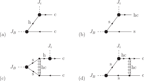
Figure 1: Examples for different momentum configurations that contribute to the $B\to\pi$ form factor in the conventional LCSR approach (“h” stands for hard, “hc” for hard-collinear, “c” for collinear, and “s” for soft interactions, using the terminology of [7]). Notice that hard interactions refer to scales of order $m_{b}$, hard-collinear interactions to scales of order $\sqrt{m_{b}\Lambda}$, and soft and collinear interactions to scales of order $\Lambda$.

In the following, we are critically re-examining the assumptions that are the basis of the LCSR approach to exclusive $B$ decays. As the simplest example we consider the $B\to\pi$ form factor at large recoil. Representing the $B$ meson by a pseudoscalar current

$$J_{B}(x)=\bar{b}(x)i\gamma_{5}q^{\prime}(x)\,,$$

one considers the correlation function

$$\Pi_{\mu}^{\rm QCD}(p_{B},p^{\prime}{}) = i\int d^{4}x\,e^{-ip_{B}x}\,\langle\pi(p^{\prime}{})|T[J_{B}(x)J_{\mu}(0)]|0\rangle\,.$$ (12)

The perturbative calculation of the correlation function requires large negative values,

$$p_{B}^{2}-m_{b}^{2}\ll 0\ .$$

On the other hand, in the sum rule one needs the imaginary part of the correlation function at values for $p_{B}^{2}$ close to the threshold parameter where

$$p_{B}^{2}-m_{b}^{2}=2m_{b}\omega_{0}$$

The scaling of the threshold parameter $\omega_{0}$ has to be chosen as

$$\Lambda_{\rm QCD}\ll\omega_{0}\sim\Lambda\ll m_{b}\,.$$

such that the “soft” scale $\Lambda$ can be interpreted as a perturbative scale in the low-energy effective theory (SCET_II).

Let us first consider the diagrams in Fig. 1(a,b) which contribute to the imaginary part of the correlation function ${\rm Im}[\Pi(\omega_{0})]$ at tree-level. Let us parametrize the momentum of the light quark entering $J_{B}$ as

$$p^{\mu}_{\bar{q}} = \bar{u}(n_{+}p^{\prime})\,\frac{n_{-}^{\mu}}{2}-p_{\perp}^{\mu}+\frac{p_{\bar{q}}^{2}-p_{\perp}^{2}}{\bar{u}\,(n_{+}p^{\prime})}\frac{n_{+}^{\mu}}{2}\,,$$ (13)

where $\bar{u}=1-u$ denotes the longitudinal momentum fraction, the transverse momentum components satisfy $n_{\pm}p_{\perp}=0$, and the virtuality scales as $|p_{\bar{q}}^{2}|\sim|p_{\perp}^{2}|\sim\Lambda^{2}$. Choosing a frame where $(p_{\perp}p_{B})=0$ and $(n_{\pm}p_{B})\sim m_{b}$, the denominator of the heavy-quark propagator in momentum space reads

$$(p_{B}-p_{\bar{q}})^{2}-m_{b}^{2}=2m_{b}\omega_{0}-\bar{u}(n_{-}p_{B})(n_{+}p^{\prime})-\frac{p_{\bar{q}}^{2}-p_{\perp}^{2}}{\bar{u}\,(n_{+}p^{\prime})}(n_{+}p_{B})+p_{\bar{q}}^{2}\,.$$

Generic parton configurations in the pion are classified as collinear, and characterized by $u,\bar{u}={\cal O}(1)$. This case corresponds to the diagram in Fig. 1(a), and allows us to approximate

generic $$: \qquad(p_{B}-p_{\bar{q}})^{2}-m_{b}^{2}=-\bar{u}\,(n_{-}p_{B})(n_{+}p^{\prime})+{\cal O}(m_{b}\Lambda)\,,$$ (14)

from which we see that:

• the heavy quark propagates on short distances, of order $1/m_{b}$, which would suggest a perturbative treatment of the correlation function in terms of $\alpha_{s}(m_{b})$;

• the non-locality of the correlation function is determined by $\bar{u}(n_{+}p^{\prime})$, which only involves the momentum components collinear to the light-hadron momentum $p^{\prime}{}$ which reflects the dominance of light-like separations.

The situation is different if we approach end-point configurations where $\bar{u}$ is small, $\bar{u}={\cal O}(\Lambda/m_{b})$. At tree level this corresponds to the diagram in Fig. 1(b), where the spectator quark is soft and, by momentum conservation, the light quark from the heavy-quark decay is hard-collinear. Notice that in the heavy-quark limit this situation is enforced by the Borel transformation which actually suppresses $b$-quark virtualities $p_{b}^{2}-m_{b}^{2}\gg\Lambda m_{B}$ (in particular it suppresses the configurations in Fig. 1(a)). In this case we have

end-point $$: \quad(p_{B}-p_{\bar{q}})^{2}-m_{b}^{2}$$ (16)

$$\quad=2m_{b}\omega_{0}-\bar{u}(n_{-}p_{B})(n_{+}p^{\prime})-\frac{p_{\bar{q}}^{2}-p_{\perp}^{2}}{\bar{u}\,(n_{+}p^{\prime})}(n_{+}p_{B})+{\cal O}(\Lambda^{2})\,.$$

Also,

• the heavy quark propagates at distances of order $1/\Lambda$ (as in HQET, the virtuality of the heavy quark propagator is of order $\Lambda m_{b}$, but the residual heavy-quark momentum is of order $\Lambda$). These configurations are unsuppressed by the Borel transformation, and suggest a perturbative expansion in terms of $\alpha_{s}(\Lambda)$.

• The correlation function is not necessarily dominated by light-like distances, as can be seen by the appearance of the (supposed-to-be) sub-leading momentum component $(n_{-}p_{\bar{q}})=\frac{p_{\bar{q}}^{2}-p_{\perp}^{2}}{\bar{u}(n_{+}p^{\prime})}$. In this case, the convergence of the light-cone expansion is not related to the $\Lambda/m_{b}$ power counting. Instead, in the above example, one has an expansion based on the formal power-counting $|p_{\bar{q}}^{2}-p_{\perp}^{2}|\sim\Lambda_{\rm QCD}^{2}\ll\Lambda^{2}$. After Borel transformation it translates into an expansion in inverse powers of the Borel parameter.

Finally, the momentum configurations in Fig. 1(c,d) contain the factorizable form-factor contributions. For these situations, Ball [23] has shown that the traditional LCSRs and the QCD factorization approach [11] to the $B\to\pi$ form factors lead to the same result. Here, the light-cone separation of the two quark fields in the pion follows from the structure of the hard-collinear propagators. The perturbative expansion is thus in terms of $\alpha_{s}(\mu_{\rm hc})$, and in this case one observes the suppression of higher-twist LCDAs of the pion by $1/m_{b}$.

We conclude that the description of the end-point contributions to the (“soft”) $B\to\pi$ form factor within LCSR in the heavy-quark limit shows similar subtleties as in the QCD factorization approach [11]. This is related to the fact that in the heavy-quark limit the light-cone sum rule is dominated by diagrams like in Fig. 1(b), which do not correspond to the parton configurations that one would usually associate with LCDAs of the pion. Although, for finite heavy-quark masses, one finds a numerical stability of the result with respect to the sum rule parameters and the twist expansion, the predictions for the “soft” end-point contributions should thus be interpreted with some care. Even if one accepts the formal derivation on the basis of the light-cone expansion of the correlation function as a sufficiently good approximation, the problem can easily be identified on the practical level: for generic parton configurations (related to the factorizable contributions in the heavy quark limit) the basic non-perturbative object is the moment

$$\langle u^{-1}\rangle_{\pi} \equiv \int du\,\frac{\phi_{\pi}(u)}{u}=3\left(1+a_{2}+a_{4}+\ldots\right)$$ (17)

of the leading-twist LCDA of the pion. Here we also indicated the expansion in terms of Gegenbauer coefficients. Notice that the coefficients in front of the $a_{n}$ for this case is 1 for all $n$, and therefore, in practice, the expansion can be truncated under the assumption that the coefficients $a_{n}$ decrease with $n$. On the other hand, as explained above, the end-point contributions in the heavy-quark limit involve, for instance, the quantity

$$\phi_{\pi}^{\prime}(1)=-6\left\{1+6a_{2}+15a_{4}+\ldots+\mbox{$\left(\begin{array}[]{c}n+2\\ 2\end{array}\right)$}\,a_{n}+\ldots\right\}\,.$$ (20)

where the coefficients in front of the $a_{n}$ now grow quadratically with $n$. For completeness, we also quote the expression for the value at the symmetric point $u=1/2$, which can be constrained from light-cone sum rules [27],

$$\phi_{\pi}(1/2)=\frac{3}{2}\left(1-\frac{3}{2}a_{2}+\frac{15}{8}a_{4}+\ldots\right)\,.$$ (21)

For this quantity the coefficients in front of the $a_{n}$ grow as $\sqrt{n}$ for large $n$.

Figure 2: The pion LCDA $\phi_{\pi}(u)$ as a function of the longitudinal momentum fraction $u$ for the examples quoted in the text – solid lines. For comparison we have also shown the asymptotic LCDA $\phi_{\pi}(u)=6u(1-u)$ – dashed line.

The notation suggests that the two quantities $\langle u^{-1}\rangle_{\pi}$ (or $\phi_{\pi}(1/2)$) and $\phi_{\pi}^{\prime}(1)$ can be derived from one and the same quantity, $\phi_{\pi}(u)$, which could be true if $\phi_{\pi}(u)$ were exactly known. However, in practice, we only have limited information on that function. Usually, one can constrain the first few Gegenbauer coefficients from experimental data (for instance the $\pi\gamma$ form factor), or from sum rules for the first few moments of $\phi_{\pi}(u)$ or for $\phi_{\pi}(1/2)$ (see [28] for a recent discussion and more references). Let us assume that we approximate $\phi_{\pi}(u)$ by keeping only the two terms $a_{2}$ and $a_{4}$ in the Gegenbauer expansion. As explained above, we can determine the values for $a_{2}$ and $a_{4}$ only to some accuracy. The following table compares two not unrealistic cases:

Case	$\langle u\rangle_{\pi}$	$\langle u^{2}\rangle_{\pi}$	$\langle u^{3}\rangle_{\pi}$	$\langle u^{4}\rangle_{\pi}$	$\langle u^{-1}\rangle_{\pi}$	$\phi_{\pi}(1/2)$	$\phi_{\pi}^{\prime}(1)$
$\matrix{a_{2}=-0.05\\ a_{4}=-0.05}$	1/2	0.30	0.19	0.14	2.70	1.47	-20.3
$\matrix{a_{2}=\phantom{-}0.10\\ a_{4}=\phantom{-}0.05}$	1/2	0.31	0.21	0.16	3.45	1.42	-14.1

The variation of the lowest-order moments $\langle u^{n}\rangle_{\pi}$ and of $\phi_{\pi}(1/2)$ in these cases is of the order of only 10%, whereas neither the sign nor the order of magnitude of $\phi_{\pi}^{\prime}(1)$ can be reliably estimated in this way. In Fig. 2 we have illustrated the shape of the function $\phi_{\pi}(u)$ for these cases, compared to the asymptotic LCDA (which corresponds to $\phi_{\pi}(u)=6u(1-u)$, $\langle u^{-1}\rangle_{\pi}=3$, and $\phi_{\pi}^{\prime}(1)=-6$). Notice, that although our choices for $a_{2}$ and $a_{4}$ are more or less ad hoc, the range of “allowed” or reasonable LCDAs is quite similar to the ones obtained from the set of models proposed in [28], where the issue of how to constrain $\phi_{\pi}(u)$ is discussed in more detail.

It follows that for a conservative numerical analysis of the LCSRs in the heavy-quark limit, one should rather consider $\phi^{\prime}_{\pi}(1)$ as an independent non-perturbative parameter. Physically, this is related to the fact that $\phi_{\pi}^{\prime}(1)$ describes completely different momentum configurations than $\phi_{\pi}(u)$ and its moments. Technically, it is impossible to re-construct the value of $\phi_{\pi}^{\prime}(1,\mu_{0})$ and its evolution under renormalization from a finite number of moments of $\phi_{\pi}(u,\mu_{0})$, where $\mu_{0}$ is a hadronic scale. This implies that, at the moment, the predictions for the very end-point contributions in LCSR may have uncertainties larger than usually considered: in the tree-level contribution to the form factor $f_{+}(0)\approx 0.3$, the above example corresponds to an uncertainty of about $0.4$, i.e. a 100% effect (for $\omega_{0}\simeq 1$ GeV). Notice, that the situation becomes even worse if we allow for (small) non-zero values for $a_{6}$, $a_{8}$ etc. This implies that for a quantitative analysis of the theoretical uncertainty coming from the hadronic input functions $\phi_{\pi}$ and $\phi_{P}$, it is generally not sufficient to only vary $a_{2}$ and $a_{4}$, at least in case of the soft form factor in the heavy-quark limit. This observation may solve the apparent problem which has been identified in [23], where an unacceptably large value for the $B\to\pi$ form factor has been obtained in the heavy-quark limit.

We should emphasize again that the above criticism applies to the very limit $m_{b}\to\infty$ in QCD light-cone sum rules. For finite heavy-quark masses (which are usually considered) the sensitivity to the end-point region appears to be small. Still, the latter statement requires verification, and we would like to propose to study the end-point configurations in QCD light-cone sum rules more carefully, and to consider the independent values of $\phi^{\prime}_{\pi}(1)$ and $\phi_{P}(1)$ as additional sources of systematic uncertainties. It is also true that for finite heavy-quark masses it is not mandatory to resum large logarithms $\ln m_{b}/\Lambda$. The prize one has to pay is that at higher orders in the perturbative expansion the soft form factor potentially involves more and more contributions from higher-twist wave functions, and that the choice of the renormalization scale has to account for a rather large range, say between 1 GeV and $2m_{b}$. Again, as long as the expansion in inverse powers of the Borel parameter ($\Lambda_{\rm QCD}/\Lambda$) is numerically well-behaved and the perturbative corrections are reasonably small, this does not question the present result for the central values of the $B\to\pi$ form factor, but may lead to some enhancement of theoretical uncertainties (see also [29] for a recent update of $B$-meson form factors within the sum-rule approach).

On the other hand, in the heavy-quark limit, a systematic study of radiative corrections does require the logarithms related to the hard scale $m_{b}$ to be separated from those related to the hard-collinear scale $\mu_{\rm hc}\sim\sqrt{\Lambda m_{b}}$. As we will show below, the effective-theory framework provides a consistent tool to achieve the perturbative separation of scales. The sum-rule techniques can then be applied to correlation functions in the effective theory (SCET_I) itself. This will automatically lead to the separation of soft and collinear fields along the light-cone, which is a built-in feature of the SCET Feynman rules and related to the power-counting of fields and operators in the effective Lagrangian in terms of a small parameter $\lambda=\sqrt{\Lambda/m_{b}}$ which formally vanishes in the limit $m_{b}\to\infty$. Our formalism does not require an additional twist expansion of correlation functions in SCET. In this framework it is possible to systematically control the renormalization-scale dependence of correlation functions, and to consistently resum large logarithms $\ln m_{b}/\mu_{\rm hc}$ for both, generic and end-point configurations. The power corrections from $\Lambda/m_{B}$-suppressed contributions, on the other hand, are hard to estimate at present. Therefore, the advantages and disadvantages of the traditional LCSRs and the SCET sum rules, which we are going to derive, are to be viewed as complementary.

3 Sum rules in SCET

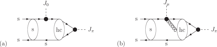
Figure 3: Contribution to the “soft” form factor $\xi_{\pi}$ (a) and to the QCD-factorizable contribution from hard-collinear spectator scattering (b) to the SCET sum rule in the heavy-quark limit (additional soft spectators are not drawn). The soft interactions, denoted by the ellipse on the left-hand side, are parametrized by the light-cone wave function of the $B$ meson.

Within SCET (more precisely SCET_I, which is the effective theory describing the interaction of soft fields and hard-collinear fields with virtuality $\Lambda m_{b}$), the non-factorizable (i.e. end-point-sensitive) part of the $B\to\pi$ form factor in the heavy-quark limit is described by the current operator

$$J_{0}(0)=\bar{\xi}_{\rm hc}(0)W_{\rm hc}(0)Y_{s}^{\dagger}(0)h_{v}(0)\,,$$

where $\xi_{\rm hc}$ is the “good” light-cone component of the light-quark spinor with $n\hskip-5.0pt/_{-}\xi_{\rm hc}=0$, and $W_{\rm hc}$ and $Y_{s}^{\dagger}$ are hard-collinear and soft Wilson lines (the latter appear after one decouples soft gluons from the leading-power hard-collinear Lagrangian, which is convenient for the following discussion). Finally, $h_{v}$ is the usual HQET field. As we have seen in the previous Section, the heavy quark is nearly on-shell in the end-point region. In SCET_I this is reflected by the fact that hard sub-processes (virtualities of order $m_{b}^{2}$) are already integrated out and appear in coefficient functions multiplying $J_{0}$. Consequently, the heavy quark should better be treated as an external field and not as a propagating particle in the correlation function. In the SCET sum rules to be derived below, we therefore will not introduce an interpolating current for the $B$ meson. Instead, the short-distance (off-shell) modes in SCET_I are the hard-collinear quark and gluon fields, and therefore the sum rules should be derived from a dispersive analysis of the correlation function

$$\Pi(p^{\prime}) = i\int d^{4}x\,e^{ip^{\prime}{}x}\,\langle 0|T[J_{\pi}(x)J_{0}(0)]|B(p_{B})\rangle\,,$$ (22)

where $p_{B}^{\mu}=m_{B}v^{\mu}$, and

$$J_{\pi}(x) \equiv -i\,\bar{\psi}(x)\,n\hskip-5.0pt/_{+}\gamma_{5}\,\psi(x)$$ (23)

$$= -i\,\bar{\xi}_{\rm hc}(x)\,n\hskip-5.0pt/_{+}\gamma_{5}\,\xi_{\rm hc}(x)-i\,\left(\bar{\xi}_{\rm hc}W_{\rm hc}(x)n\hskip-5.0pt/_{+}\gamma_{5}Y_{s}^{\dagger}q_{s}(x)+h.c.\right)\,.$$

Here we denoted quark fields in QCD as $\psi$ and soft and hard-collinear quark fields in SCET as $q_{s}$ and $\xi_{\rm hc}$, respectively [6]. Notice that soft-collinear interactions require a multi-pole expansion of soft fields [6] which is always understood implicitly. We also point out that the effective theory SCET_I contains SCET_II as its infrared limit (i.e. when the virtuality of the hard-collinear modes is lowered to order $\Lambda^{2}$). For this reason, the hard-collinear fields which define the interpolating current $J_{\pi}$ also contain the collinear configurations which show up as hadronic bound states (see also the discussion in [7]).

According to the discussion in Section 3.4 of the first reference in [6], the above expression for $J_{\pi}$, which has been derived from the tree-level matching of QCD onto SCET_I will not receive any radiative corrections since there is no hard scale (which could have entered only through the heavy-$b$-quark mass). The pion-to-vacuum matrix element of the current $J_{\pi}$ is thus given as

$$\langle 0|J_{\pi}|\pi(p^{\prime})\rangle = (n_{+}p^{\prime})\,f_{\pi}\,.$$ (24)

In the following we will consider a reference frame where $p^{\prime}_{\perp}=v_{\perp}=0$ and $n_{+}v=n_{-}v=1$. In this frame the two independent kinematic variables are

$$(n_{+}p^{\prime}{})\simeq 2E_{\pi}={\cal O}(m_{b})\,,\qquad 0>(n_{-}p^{\prime}{})={\cal O}(\Lambda)\,,$$ (25)

with $|n_{-}p^{\prime}|\gg m_{\pi}^{2}/(n_{+}p^{\prime})$. The dispersive analysis will be performed with respect to $(n_{-}p^{\prime})$ for fixed values of $(n_{+}p^{\prime})$.

3.1 Tree-level result

Figure 4: (a) Leading contribution to the correlation function for the non-factorizable SCET current $J_{0}$. (b) Leading contribution for the factorizable SCET current $J_{1}$ (see below).

At leading power, the tree-level result, see Fig. 4(a), for the correlation function involves one hard-collinear quark propagator, which reads

$$S_{F}^{\rm hc}=\frac{i}{n_{-}p^{\prime}{}-\omega+i\eta}\,\frac{n\hskip-5.0pt/_{-}}{2}\,,$$ (26)

where $\omega=n_{-}k$, and $k^{\mu}$ is the momentum of the soft light quark that will end up as the spectator quark in the $B$ meson. In contrast to the situation discussed in Section 2, the light-cone dominance in the SCET sum rules (now between the soft constituents of the $B$ meson) follows from the structure of SCET itself and does not constitute an additional assumption.

The perturbative evaluation of the SCET correlation function follows from contracting hard-collinear fields. This leads to matrix elements of operators that are formulated only in terms of soft fields, which are separated along the light cone and thus define light-cone distribution amplitudes for the $B$ meson in HQET [11]. Using the momentum-space representation of LCDAs for $B$ mesons as in [14, 11],

$${\cal M}^{B}_{\beta\alpha}=-\frac{if_{B}m_{B}}{4}\left[\frac{1+v\hskip-5.0pt/}{2}\left\{\phi_{+}^{B}(\omega)n\hskip-5.0pt/_{+}+\phi_{-}^{B}(\omega)n\hskip-5.0pt/_{-}+\ldots\right\}\gamma_{5}\right]_{\beta\alpha}\,,$$

we find

$$\Pi(n_{-}p^{\prime}{}) = f_{B}m_{B}\int_{0}^{\infty}d\omega\,\frac{\phi_{-}^{B}(\omega)}{\omega-n_{-}p^{\prime}{}-i\eta}\,.$$ (27)

The considered correlation function in the (unphysical) Euclidean region thus factorizes into a perturbatively calculable hard-collinear kernel and a soft light-cone wave function for the $B$-meson, where the convolution variable $\omega$ represents the light-cone momentum of the spectator quark in the $B$-meson. We will show below that this factorization still holds after including radiative corrections in SCET_I.

The result (27) already has the form of a dispersion integral in the variable $n_{-}p^{\prime}$

$$\Pi(n_{-}p^{\prime}) = \frac{1}{\pi}\int_{0}^{\infty}d\omega^{\prime}\,\frac{{\rm Im}[\Pi(\omega^{\prime})]}{\omega^{\prime}-n_{-}p^{\prime}-i\eta}\,.$$ (28)

The Borel transform with respect to the variable $n_{-}p^{\prime}{}$ introduces the Borel parameter $\omega_{M}$ and reads

$$\hat{B}\left[\Pi\right](\omega_{M}) = \frac{1}{\pi}\int_{0}^{\infty}d\omega^{\prime}\,\frac{1}{\omega_{M}}\,e^{-\omega^{\prime}/\omega_{M}}\,{\rm Im}[\Pi(\omega^{\prime})]$$ (29)

$$= f_{B}m_{B}\int_{0}^{\infty}d\omega\,\frac{1}{\omega_{M}}\,e^{-\omega/\omega_{M}}\,\phi_{-}^{B}(\omega)\,.$$ (30)

The physical role of the Borel parameter is to enhance the contribution of the hadronic-resonance region where the virtualities of internal propagators have to be smaller than the hard-collinear scale. The dependence of the sum rule on $\omega_{M}\sim\Lambda^{2}/(n_{+}p^{\prime})$ will later be used to quantify the model-dependence of our result. On the hadronic side, one can write

$$\Pi^{\rm HAD}(n_{-}p^{\prime})=\Pi(n_{-}p^{\prime})\Big{|}_{\rm res.}+\Pi(n_{-}p^{\prime})\Big{|}_{\rm cont.}\,,$$ (31)

where the first term represents the contribution of the pion, while the second takes into account the role of higher states and continuum above an effective threshold $\omega_{s}={\cal O}(\Lambda^{2}/n_{+}p^{\prime})$. Using (4) and (24), the pion contribution to the dispersive integral is given by

$$\Pi(n_{-}p^{\prime})\Big{|}_{\rm res.} = \frac{\langle 0|J_{\pi}|\pi(p^{\prime})\rangle\langle\pi(p^{\prime})|J_{0}|B(p_{B})\rangle}{m_{\pi}^{2}-p^{\prime}{}^{2}}\ =\ \frac{(n_{+}p^{\prime})^{2}\,\xi_{\pi}(n_{+}p^{\prime})\,f_{\pi}}{m_{\pi}^{2}-p^{\prime}{}^{2}}\,.$$ (32)

Neglecting the pion mass and in the chosen frame where $p^{\prime}_{\perp}=0$, one has

$$\Pi(n_{-}p^{\prime})\Big{|}_{\rm res.}=-{(n_{+}p^{\prime})\xi_{\pi}(n_{+}p^{\prime})f_{\pi}\over n_{-}p^{\prime}}$$ (33)

and hence

$$\hat{B}\left[\Pi\right](\omega_{M})\Big{|}_{\rm res.}={(n_{+}p^{\prime})\xi_{\pi}(n_{+}p^{\prime})f_{\pi}\over\omega_{M}}\,.$$ (34)

On the other hand, $\Pi(n_{-}p^{\prime})\Big{|}_{\rm cont.}$ can be written again according to a dispersion relation analogous to (28) where, assuming global quark-hadron duality, we identify the spectral density with its perturbative expression, obtaining:

$$\hat{B}\left[\Pi\right](\omega_{M})\Big{|}_{\rm cont.} = \frac{1}{\pi}\int_{\omega_{s}}^{\infty}d\omega^{\prime}\,\frac{1}{\omega_{M}}\,e^{-\omega^{\prime}/\omega_{M}}\,{\rm Im}[\Pi(\omega^{\prime})]$$ (35)

$$= f_{B}m_{B}\int_{\omega_{s}}^{\infty}d\omega\,\frac{1}{\omega_{M}}\,e^{-\omega/\omega_{M}}\,\phi_{-}^{B}(\omega)\,.$$ (36)

This term can finally be subtracted from (28), giving the final sum rule

$$\xi_{\pi}(n_{+}p^{\prime}) = \frac{1}{f_{\pi}(n_{+}p^{\prime})}\,\int_{0}^{\omega_{s}}d\omega^{\prime}\,e^{-\omega^{\prime}/\omega_{M}}\,{1\over\pi}{\rm Im}[\Pi(\omega^{\prime})]\,.$$ (37)

At tree level in SCET the previous equation becomes:

$$\xi_{\pi}(n_{+}p^{\prime}) = \frac{f_{B}m_{B}}{f_{\pi}(n_{+}p^{\prime})}\,\int_{0}^{\omega_{s}}d\omega\,e^{-\omega/\omega_{M}}\,\phi_{-}^{B}(\omega)\qquad\mbox{(tree level)}\,.$$ (38)

The dependence of $\phi_{-}^{B}(\omega)$ occurs on scales $\omega_{0}={\cal O}(\Lambda)$. For small values of the threshold parameter, $\omega_{s}\ll\Lambda$, one can approximate

$$\xi_{\pi}(n_{+}p^{\prime}) \simeq \frac{f_{B}m_{B}}{f_{\pi}n_{+}p^{\prime}}\,\phi_{-}^{B}(0)\,\int_{0}^{\omega_{s}}d\omega\,e^{-\omega/\omega_{M}}$$ (39)

$$= \frac{m_{B}\omega_{M}}{f_{\pi}(n_{+}p^{\prime})}\left(1-e^{-\omega_{s}/\omega_{M}}\right)\,f_{B}\phi_{-}^{B}(0)\,\qquad\mbox{(tree level, approx.)}\,.$$

3.2 Comments

• The result for $\xi_{\pi}$ has the correct scaling with $\Lambda/m_{B}$ as obtained from the conventional sum rules or from the power counting in SCET.

• The factorizable contributions in exclusive $B$-meson decays usually contain the first inverse moment of the $B$-meson distribution amplitude $\phi_{+}^{B}(\omega)$:

  $$\lambda_{B}^{-1}=\int_{0}^{\infty}d\omega\,\frac{\phi_{+}(\omega)}{\omega}$$

  On the other hand, the soft form factor is proportional to $\phi_{-}^{B}(0)$. In the Wandzura-Wilczek (WW) approximation, the two quantities are directly related [11],

  $$\phi_{-}^{B}(0) \simeq \int_{0}^{\infty}d\omega\,\frac{\phi_{+}^{B}(\omega)}{\omega}\qquad\mbox{(WW)}\,.$$ (40)

  Thus the situation is different from the case discussed in Section 2, where, considering the heavy-quark limit, the non-perturbative parameters appearing in the hard-scattering and in the soft contributions are not directly related to each other. It should, however, be mentioned that the above relation is modified by 3-particle Fock states with one additional soft gluon in the $B$ meson. The sensitivity of the soft form factor on $\phi_{-}^{B}(\omega)$ and three-particle LCDAs has also been observed in the context of QCD factorization [30, 31, 7].

• At tree level, QCD and SCET are indistinguishable, and therefore our result in (39) can also be derived using the full QCD Feynman rules [32]. For the comparison, one has to identify $M^{2}=\omega_{M}\,(n_{+}p^{\prime})$ and $s_{0}=\omega_{s}\,(n_{+}p^{\prime})$. Notice that the organization of radiative corrections is different in the two frameworks. Also the behaviour of the form factor as a function of $q^{2}$ depends on the exact treatment of $(\omega_{s},\omega_{M})$. The standard treatment corresponds to $s_{0},M^{2}={\rm const.}$, in which case the soft form factor (at tree-level) scales as $1/(n_{+}p^{\prime})^{2}$.

  One non-trivial issue concerns the hard matching coefficients between the heavy-to-light currents $\bar{q}\Gamma_{i}Q$ in QCD and $J_{0}$ in SCET. They induce a renormalization-scale dependence, which to NLL accuracy has the universal evolution [5]:

  $$C_{i}(\mu) \simeq C_{i}(m_{b})\,\exp\left[-\frac{4\pi C_{F}}{\beta_{0}^{2}\,\alpha_{s}(m_{b})}\left(\frac{1}{z}-1+\ln z\right)+f_{1}(z)\right]\,,$$ (41)

  $$z^{-1} = 1+\frac{\beta_{0}}{2\pi}\,\alpha_{s}(m_{b})\,\ln\frac{\mu}{m_{b}}\,.$$ (42)

  The first term in the exponent resums the Sudakov double logarithms ($\alpha_{s}\,\ln^{2}\mu$, …) between the scales $m_{b}$ and $\mu$. The function $f_{1}(z)$ , which takes into account NLL effects ($\alpha_{s}\,\ln\mu$, $\alpha_{s}^{2}\ln^{2}\mu$, …) , can be found in [5].

3.3 Radiative corrections from hard-collinear loops

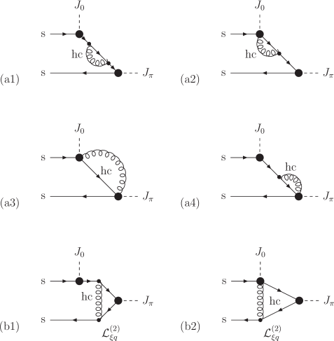
Figure 5: Diagrams contributing to the sum rule for $\xi_{\pi}$ to order $\alpha_{s}$ with hard-collinear loops and no external soft gluons. Diagrams (a2-a4) and (b2) vanish in light-cone gauge $n_{+}A_{\rm hc}=0$. Diagram (a3) vanishes both in light-cone and in Feynman gauge.

In SCET short-distance radiative corrections to the correlation function (22) are represented by hard-collinear loops, as shown in Fig. 5 for the leading order in $\alpha_{s}$. The diagrams denoted by (a1-a4) and (b1-b2) form gauge-invariant subsets, such that before the Borel transformation the result for the correlation function reads

$$\Pi(n_{-}p^{\prime},\epsilon) = f_{B}m_{B}\int_{0}^{\infty}d\omega\,\frac{\phi_{-}^{B}(\omega)}{\omega-n_{-}p^{\prime}{}-i\eta}\left\{1+\frac{\alpha_{s}C_{F}}{4\pi}\left(\mbox{(a1-a4)}+\mbox{(b1-b2)}\right)\right\}\,.$$ (43)

We obtain

(a1-a4) $$= \frac{4}{\epsilon^{2}}+\frac{1}{\epsilon}\,(3+4L_{0}-4L_{1}(\omega))$$ (46)

$$\quad+L_{0}\left(3+2L_{0}-4L_{1}(\omega)\right)-L_{1}(\omega)\left(3-2L_{1}(\omega)\right)+7-\frac{\pi^{2}}{3}\,,$$

and

(b1-b2) $$= -\frac{2}{\epsilon^{2}}-\frac{1}{\epsilon}\left(1+2L_{0}+2L_{1}(\omega)\left(1-\frac{n_{-}p^{\prime}}{\omega}\right)\right)$$ (49)

$$\ -L_{0}\left(1+L_{0}+2L_{1}(\omega)\left(1-\frac{n_{-}p^{\prime}}{\omega}\right)\right)$$

$$-L_{1}(\omega)(3-L_{1}(\omega))\left(1-\frac{n_{-}p^{\prime}}{\omega}\right)-3+\frac{\pi^{2}}{6}\,,$$

where we have defined the abbreviations

$$L_{0}=\ln\left[\frac{\mu^{2}}{(n_{+}p_{\pi})(-n_{-}p^{\prime}-i\eta)}\right]\,,\qquad L_{1}(\omega)=\ln\left[1-\frac{\omega}{n_{-}p^{\prime}+i\eta}\right]\,.$$ (51)

Notice that the hard-scattering diagrams (b1-b2) involve a sub-leading term in the SCET Lagrangian, describing the interactions of soft and hard-collinear quarks [6]:

$${\cal L}_{\xi q}^{(2)} = \bar{q}_{s}W_{\rm hc}^{\dagger}(in_{-}D_{\rm hc}+iD\hskip-6.49994pt/_{\perp\rm hc}\,(in_{+}D_{\rm hc})^{-1}\,iD\hskip-6.49994pt/_{\perp\rm hc})\frac{n\hskip-5.0pt/_{+}}{2}\,\xi+\ldots$$ (52)

(The insertion of ${\cal L}_{\xi q}^{(1)}$ vanishes by rotational invariance in the transverse plane.)

3.4 Renormalization-scale dependence of the correlator

The renormalization-scale dependence for the correlation function in (22) comes from three sources. Let us, for the moment, focus on the leading double-logarithmic terms:

• The hard-collinear loop contributions yield

  $$\frac{\alpha_{s}C_{F}}{4\pi}\,\frac{\partial}{\partial\ln\mu}\,\mbox{(a1-a4)}^{\overline{\rm MS}} = \frac{\alpha_{s}C_{F}}{4\pi}\left(8\ln\frac{\mu^{2}}{\mu_{\rm hc}^{2}}+\mbox{$\mu$-independent terms}\right)\,,$$ (53)

  and

  $$\frac{\alpha_{s}C_{F}}{4\pi}\,\frac{\partial}{\partial\ln\mu}\,\mbox{(b1-b2)}^{\overline{\rm MS}} = \frac{\alpha_{s}C_{F}}{4\pi}\left(-4\ln\frac{\mu^{2}}{\mu_{\rm hc}^{2}}+\mbox{$\mu$-independent terms}\right)\,.$$ (54)

• The evolution equation of the $B$-meson LCDA (see [33, 34] and Eq. (LABEL:softdiff) in Appendix A.3) implies

  $$\frac{\partial}{\partial\ln\mu}\,\int d\omega\,\frac{\phi_{-}^{B}(\omega,\mu)}{\omega-n_{-}p^{\prime}} = \frac{\alpha_{s}C_{F}}{4\pi}\,\int d\omega\,\frac{\phi_{-}^{B}(\omega,\mu)}{\omega-n_{-}p^{\prime}}\left(-2\ln\frac{\mu^{2}}{\mu_{0}^{2}}+\mbox{$\mu$-independent terms}\right)\,.$$ (55)

  Here, we have used the fact that the anomalous-dimension kernel for $B$-meson LCDAs contains a universal term related to the cusp anomalous dimension:

  $$\gamma_{\pm}(\omega,\omega^{\prime},\mu)=\Gamma_{\rm cusp}(\alpha_{s})\,\ln\frac{\mu}{\mu_{0}}\,\delta(\omega-\omega^{\prime})+\mbox{$\mu$-independent terms}\,,$$ (57)

  with $\Gamma_{\rm cusp}=4+{\cal O}(\alpha_{s})$.

• The evolution of the $B$-meson decay constant $f_{B}(\mu)$ in HQET does not contain Sudakov double logs.

As required, the resulting scale-dependence of the correlation function cancels with those of the Wilson coefficients $C_{i}(\mu)$ in (42) to the considered leading logarithmic order (which involves the Sudakov double logs),

$$\frac{\partial}{\partial\ln\mu}\,C_{i}(\mu) = \frac{\alpha_{s}C_{F}}{4\pi}\left(-2\ln\frac{\mu^{2}}{m_{b}^{2}}+\mbox{$\mu$-independent terms}\right)\,C_{i}(\mu)\,.$$ (58)

To show the cancellation of the sub-leading single-logarithmic terms, we would have to compute the $\mu$-independent terms in the anomalous-dimension function $\gamma_{-}(\omega,\omega^{\prime})$ as well as the finite $\alpha_{s}$ corrections from the diagrams shown in Fig. 6 (the NLL term in $C_{i}(\mu)$ is known [5]). Notice that to NLL accuracy also the WW approximation will receive corrections from the three-particle $B$-meson LCDA, with one additional soft transverse gluon, see the discussion in Appendix A.3. We will leave the cancellation of single logs and the corrections from three-particle LCDAs for future investigations.

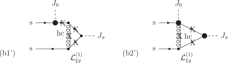
Figure 6: $\alpha_{s}$ corrections from hard-collinear loops involving an additional transverse soft gluon. The crosses indicate possible insertions of the corresponding interactions with soft gluons from the sub-leading SCET Lagrangian, ${\cal L}_{\xi}^{(1)}$ and ${\cal L}_{\rm YM}^{(1)}$.

It is to be stressed that, for the hard-collinear loop diagrams, the power counting in SCET requires at least one insertion of the sub-leading Lagrangian ${\cal L}^{(1)}$ for kinematical reasons, and the coupling of external transverse soft gluons to hard-collinear particles costs another factor of $\lambda$. Therefore, in higher orders of perturbation theory, we will not encounter more than three-particle LCDAs of the $B$ meson. (Of course, the evaluation of power corrections will require a finite set of more-particle LCDAs for a given power in $\lambda$. The role of three-particle Fock states and power corrections to the $B\to\pi$ form factor is further explored in [32]. The role of four-particle Fock states in power corrections to the $B\to\pi\pi$ amplitudes has already been emphasized in [35].)

3.5 Sum rule at first order in $\alpha_{s}$

The NLO sum rule for the soft form factor is obtained from the dispersion relation (28), where we now have to include the ${\cal O}(\alpha_{s})$ corrections to the imaginary part of the correlation function. In Appendix A we have calculated the imaginary part of $\Pi(\omega^{\prime})$ resulting from the hard-collinear loop contributions in (46) and (LABEL:b12). Here we have also included the soft contributions related to the hadronic matrix element which defines the evolution of the $B$-meson LCDA $\phi_{-}^{B}(\omega,\mu)$ entering the tree-level sum rule. Using, for simplicity, the approximation $\omega_{s}\ll\Lambda$, we obtain the final sum rule to order $\alpha_{s}$,

$$\xi_{\pi}(n_{+}p^{\prime},\mu) \simeq \frac{f_{B}(\mu)m_{B}\,\phi_{-}^{B}(0,\mu_{0})}{(n_{+}p^{\prime})f_{\pi}}\,\int_{0}^{\omega_{s}}\,d\omega^{\prime}\,e^{-\omega^{\prime}/\omega_{M}}$$ (59)

$$\Bigg{\{}1+\frac{\alpha_{s}C_{F}}{4\pi}\Bigg{(}L_{0}^{\prime}(2+L_{0}^{\prime})+4+\frac{\pi^{2}}{2}+4\left(1+L_{0}^{\prime}\right)\left(\sigma_{B}(\mu_{0})-\ln\frac{\mu_{0}}{\omega^{\prime}}\right)$$

$$\qquad+\ln\frac{\mu}{\mu_{0}}\left(-4\,\sigma_{B}(\mu_{0})-2\,\ln\frac{\mu}{\mu_{0}}+2\right)\Bigg{)}\Bigg{\}}\,,$$

where $L_{0}^{\prime}=\ln[\frac{\mu^{2}}{(n_{+}p^{\prime})\,\omega^{\prime}}]$ and $\sigma_{B}(\mu_{0})$ is the logarithmic moment of the $B$-meson LCDA $\phi_{+}^{B}(\omega,\mu_{0})$ as defined in [34]. Notice, that we have neglected the effects from three-particle Fock states in the $B$-meson which would enter the sum rule at order $\alpha_{s}$, even in the WW approximation, see the discussion in Appendix A.3. In this respect, our NLO prediction is still incomplete.

3.6 QCD-factorizable contributions from SCET sum rules

In this paragraph we will show that (at least at leading-order in $\alpha_{s}$) our sum-rule approach reproduces the result for the factorizable form-factor contribution from hard-collinear spectator scattering [7, 11]. For this purpose we consider the correlation function

$$\Pi_{1}(p^{\prime}) = i\int d^{4}x\,e^{ip^{\prime}{}x}\,\langle 0|T[J_{\pi}(x)J_{1}(0)]|B(p_{B})\rangle\,,$$ (60)

where

$$J_{1} \equiv \bar{\xi}_{\rm hc}\,g\,A\hskip-5.0pt/^{\perp}_{\rm hc}\,h_{v}$$ (61)

determines the factorizable form-factor contribution $\Delta F_{\pi}$, see Appendix B. The leading contribution is given by the diagram in Fig. 4(b) which involves the insertion of one interaction vertex from the order-$\lambda$ soft-collinear Lagrangian

$${\cal L}_{\xi q}^{(1)}\ =\ \bar{\xi}_{\rm hc}\,g_{s}A\hskip-6.49994pt/_{\rm hc,\perp}\,q_{s}+\mbox{h.c.}$$

The resulting hard-collinear loop integral is UV- and IR-finite, and the correlator reads

$$\Pi_{1}(p^{\prime}) = -\,g_{s}^{2}\,C_{F}\,\,\int_{0}^{\infty}d\omega\,{\rm tr}\left[{\cal M}^{B}\,\gamma_{\mu}^{\perp}\gamma_{5}\,n\hskip-5.0pt/_{-}\gamma^{\mu}_{\perp}\right]$$ (62)

$${}\times\int\frac{d^{4}l}{(2\pi)^{4}}\frac{1}{[n_{-}l-\omega+\frac{l_{\perp}^{2}}{n_{+}l}+i\eta][n_{-}p^{\prime}+n_{-}l-\omega+\frac{l_{\perp}^{2}}{n_{+}p^{\prime}+n_{+}l}+i\eta][l^{2}+i\eta]}\,,$$

where $l^{\mu}$ is the momentum of the exchanged hard-collinear gluon. The calculation yields

$$\Pi_{1}(p^{\prime}) = -\frac{\alpha_{s}C_{F}}{4\pi}(n_{+}p^{\prime})\,\int_{0}^{\infty}d\omega\,\frac{f_{B}m_{B}\,\phi_{+}^{B}(\omega)}{\omega}\,\ln\left[1-\frac{\omega}{n_{-}p^{\prime}+i\eta}\right]\,.$$ (64)

In order to perform the Borel transformation and to define the continuum subtraction we determine the imaginary part

$$\frac{1}{\pi}\,{\rm Im}[\Pi_{1}(\omega^{\prime})] = -\frac{\alpha_{s}C_{F}}{4\pi}\,(n_{+}p^{\prime})\,\int_{0}^{\infty}d\omega\,\frac{f_{B}m_{B}\,\phi_{+}^{B}(\omega)}{\omega}\,\theta[\omega-\omega^{\prime}]\,.$$ (65)

Inserting this into the dispersion relation analogous to (28), we obtain

$$\hat{B}\left[\Pi_{1}\right](\omega_{M})\Big{|}_{\rm res.} \simeq -\frac{\alpha_{s}C_{F}}{4\pi}\,(n_{+}p^{\prime})\left(1-e^{-\omega_{s}/\omega_{M}}\right)\int_{0}^{\infty}d\omega\,\frac{f_{B}m_{B}\,\phi_{+}^{B}(\omega)}{\omega}\,,$$ (66)

where we have neglected a term which is suppressed by $\omega_{s}/\Lambda$. The hadronic expression for the same quantity reads (see Appendix B),

$$\hat{B}\left[\Pi_{1}\right](\omega_{M})\Big{|}_{\rm had.} = -\frac{\alpha_{s}C_{F}}{4\pi}\,\frac{f_{\pi}m_{B}^{2}}{2\omega_{M}}\,\Delta F_{\pi}\,.$$ (67)

Comparison with the expression for $\Delta F_{\pi}$ obtained in QCD factorization (see [11] and (116) in Appendix B) implies

$$(n_{+}p^{\prime})\,\omega_{M}\left(1-e^{-\omega_{s}/\omega_{M}}\right)=M^{2}\left(1-e^{-s_{0}/M^{2}}\right) \simeq 4\pi^{2}f_{\pi}^{2}\,,\quad\mbox{and}\quad\langle u^{-1}\rangle_{\pi}\simeq 3\,.$$ (68)

The first relation is known from the leading-order sum rule for $f_{\pi}$ (see for instance [21]). The second relation states that to the considered order the pion distribution amplitude can be approximated by the asymptotic one. Actually, in the limit $\omega_{s}\to\infty$, the result for the correlation function before the integration over $l_{\perp}$ and $n_{+}l=-\bar{u}\,(n_{+}p^{\prime})$ can be written as

$$\hat{B}\left[\Pi_{1}\right](\omega_{M}) \propto \frac{\alpha_{s}C_{F}}{4\pi}\,\left[\int_{0}^{\infty}\frac{d\omega}{\omega}\,\phi_{+}^{B}(\omega)\left(1-e^{-\omega/\omega_{M}}\right)\right]\,$$ (69)

$${}\times\left[\int_{0}^{1}\frac{du}{\bar{u}}\,\int d|l_{\perp}|^{2}\,\frac{6}{M^{2}}\,\exp\left[-\frac{|l_{\perp}|^{2}}{u\bar{u}\,M^{2}}\right]\right]\,.$$

One the one hand this explicitly shows the factorization of the soft and collinear integrations; on the other hand the structure to the right corresponds to the asymptotic wave function for the pion which is often used as a model in phenomenological applications (with $M^{2}=4\pi^{2}f_{\pi}^{2}$ for $s_{0}\to\infty$), see for instance [36, 37, 38].

A remarkable feature of the SCET-sum-rule approach to the $B\to\pi$ form factor is that the ratio of factorizable and non-factorizable contributions is independent of the $B$-meson wave function to first approximation. From (39), (40) and (117) in Appendix B we have (at $q^{2}=0$)

$$\frac{\alpha_{s}(\mu_{\rm hc})C_{F}}{4\pi}\,\frac{\Delta F(m_{B})}{\xi_{\pi}(m_{B})} \simeq \frac{\alpha_{s}(\mu_{\rm hc})C_{F}}{2\pi}\approx 6\%\,,$$ (71)

which is in line with the power counting used in QCD factorization [4, 11], but contradicts the assumptions of the so-called pQCD approach [39] and the results of a recent phenomenological study in [40].

From these considerations we see that our formalism reproduces the structure for the QCD-factorizable part of the form factor. The leading-order analysis suggests a model for the pion light-cone wave function, where the pion-distribution amplitude at the hard-collinear scale is approximated by the asymptotic form, and the transverse size of the $q\bar{q}$ Fock state in the pion is determined by the Borel parameter. Of course, these approximations should be refined by including higher-order radiative and non-perturbative corrections. For the perturbative part the accuracy can be systematically improved within the SCET framework [41, 42]. The non-perturbative uncertainties are encoded in the pion and $B$-meson distribution amplitudes at the hard-collinear scale.

4 Numerical analysis

In this Section we study the phenomenological implications of our result concerning the prediction for the $B\to\pi$ form factor in the heavy-quark limit. Our approach includes several sources of theoretical uncertainties,

• the dependence on the sum-rule parameters $\omega_{s}$ and $\omega_{M}$, including the quality of the approximation $\omega_{s},\omega_{M}\ll\Lambda$,

• the variation of the renormalization/factorization scale,

• the $B$-meson distribution amplitude $f_{B}\phi_{-}^{B}(\omega,\mu)$, in particular its value at $\omega=0$,

which we are going to address in turn.

4.1 Tree-level approximation

A priori, the threshold parameters $s_{0}=\omega_{s}\,(n_{+}p^{\prime})$ and the Borel parameter $M^{2}=\omega_{M}\,(n_{+}p^{\prime})$ are arbitrary. Their order of magnitude can be estimated from other sum rules, like the one for $f_{\pi}$ in (68). Together with (39) this defines our leading-order approximation

$$\xi_{\pi}(n_{+}p^{\prime},\mu) \simeq \frac{4\pi^{2}f_{\pi}\,f_{B}(\mu)m_{B}}{(n_{+}p^{\prime})^{2}}\,\phi_{-}^{B}(0,\mu)\,\qquad\mbox{(tree-level, default)}\,.$$ (72)

Fixing the input values at the low hadronic (soft) scale, $\mu_{0}=1$ GeV, we take $\phi_{-}^{B}(0,\mu_{0})\simeq 2.15$ GeV^-1 from [34], and $f_{B}(m_{b})=180$ MeV (which correspond to $f_{B}(\mu_{0})=150$ MeV). With this we obtain, the tree-level estimate

$$\xi_{\pi}(n_{+}p^{\prime},\mu)\approx\xi_{\pi}(n_{+}p^{\prime},\mu_{0}) \simeq 0.32\,\frac{m_{B}^{2}}{(n_{+}p^{\prime})^{2}}\,.$$ (73)

This already has the right order of magnitude that one would expect from previous studies.

4.2 Variation of the sum-rule parameters

It is to be stressed that the leading-contribution to the SCET sum rule comes from the second term in (23) which corresponds to the asymmetric momentum configuration in the pion. On the other hand, QCD sum rules for parameters like $f_{\pi}$ mainly probe the first term in (23), i.e. the symmetric configuration. Therefore, higher-order corrections to the sum rule for $\xi_{\pi}$ can be substantially different from those in $f_{\pi}$ which should be taken into account in the estimate of systematic uncertainties. We may allow for a 30% violation of the relation (68), such that

$$\frac{M^{2}\,(1-e^{-s_{0}/M^{2}})}{4\pi^{2}f_{\pi}^{2}} = 1.0\pm 0.3$$ (74)

induces a corresponding error in our estimate for $\xi_{\pi}(n_{+}p^{\prime})$. As a first estimate of the Borel and threshold parameter we start with

$$M^{2}=1~{}{\rm GeV}^{2}\,,\qquad s_{0}=1~{}{\rm GeV}^{2}\,,$$

which fulfill the relation (68). At $q^{2}=0$ this corresponds to $\omega_{M}\simeq\omega_{s}\simeq 0.2$ GeV. These values are reasonably small compared to $\Lambda$.

An additional criterion which may serve as a self-consistency check of the sum rule is to compare the (model-dependent) prediction for the continuum contribution with respect to the full sum rule. In order not to be too sensitive to the modelling of the continuum contribution by quark-hadron duality, one would like to have the ratio of the continuum and resonance contribution sufficiently small. To quantify this effect one needs a model for the shape of the $B$-meson distribution amplitude. For this study we take the simple parameterization suggested in [14]

$$\phi_{-}^{B}(\omega) = \frac{1}{\omega_{0}}\,e^{-\omega/\omega_{0}}\,,$$ (75)

with $1/\omega_{0}=\phi_{-}^{B}(0)=2.15$ GeV^-1. With this we obtain

$$r\equiv\frac{\mbox{continuum}}{\mbox{total}} = \exp\left[-\omega_{s}/\Omega_{M}\right]\,,$$ (76)

where for the starting values $\Omega_{M}=\omega_{0}\omega_{M}/(\omega_{0}+\omega_{M})\approx 0.14$ GeV, and $r\simeq 0.24$ is reasonably small. As mentioned earlier, the scaling for both the Borel parameter and for the threshold parameter is fixed as $\omega_{s}\sim\omega_{M}\sim\Lambda^{2}/M$, and therefore one always has $r<1$. We note that before the Borel transformation (which corresponds to the limit $\omega_{M}\gg\omega_{s}$) the sum rule would in fact be dominated by the continuum contribution, $r\to 1$. We see that, as usual, the Borel transformation is crucial to obtain a reasonable and self-consistent result.

A related question concerns the quality of the approximation $\omega_{s},\omega_{M}\ll\omega_{0}={\cal O}(\Lambda)$ which is only marginally fulfilled for our starting values of $M^{2}$ and $s_{0}$. In Fig. 7 we consider the tree-level sum rule and compare the ratio of the approximate result (39) and the exact formula (38) as a function of $\omega_{s}$ and $\omega_{M}$. Here we employed again the model (75). One observes that the approximate formula (solid line) tends to overestimate the exact result (dashed line) by about 15% at the “default” values for the Borel parameters. The plots also show the dependence of $\xi_{\pi}(m_{B},\mu_{0})$ on the sum rule parameters $\omega_{s}$ and $\omega_{M}$ which is substantial.

Figure 7: Dependence of the LO prediction for $\xi_{\pi}(m_{B},\mu_{0})$ on the Borel parameters. The solid line refers to the approximation $\omega_{s},\omega_{M}\ll\omega_{0}$; the dashed line denotes the exact result, see text.

At the NLO level the stability of the sum rule with respect to variation of the sum-rule parameters is improved in particular for $(\omega_{s},\omega_{M})>0.2$ GeV, see Fig. 8. From these considerations we deduce an uncertainty of $(+20\%,-30\%)$ from the variation of $\omega_{s}$ and $\omega_{M}$ (a complete stability analysis is reserved for further studies when all contributions are known and the approximation on $\omega_{s,M}$ is lifted).

Figure 8: Dependence of the form-factor prediction on the sum rule parameters at LO (dashed line) and NLO (solid line), normalized to the “default” value with $\omega_{s}=\omega_{M}=0.2$ GeV.

4.3 Renormalization-scale dependence

At tree level the question of renormalization-scale dependence reflects itself in the ambiguous choice of reference scale for the hard Wilson coefficients, and the $B$-meson distribution amplitude. Notice that only the product $C_{i}(\mu)\,\xi_{\pi}(n_{+}p^{\prime},\mu)$ should be renormalization-scale invariant. A “reasonable” choice of scale could be of the order of the hard-collinear scale, $\mu_{\rm hc}\simeq 1.5$ GeV or of the soft scale $\mu_{0}\simeq 1$ GeV. Below, we will therefore vary the scale parameter in a sufficiently large range, $\mu_{0}/2\leq\mu\leq 2\mu_{\rm hc}$.

In the tree-level approximation the renormalization-scale dependence of the product $C_{i}(\mu)\,\xi_{\pi}(n_{+}p^{\prime},\mu)$ is solely coming from the Wilson coefficients. For the range of scales indicated above we obtain

$$\frac{C_{i}(\mu)}{C_{i}(m_{b})}\big{|}_{LL} = 0.85^{+0.14}_{-0.20}\,,$$ (77)

where the central value corresponds to $\mu=\mu_{0}$. The suppression from the resummation of the Sudakov logarithms in $C_{i}(\mu)$ is moderate, of the order of at most 15-35%, but the related scale uncertainty is sizeable. This is also shown in Fig. 9(a).

At NLO, we have to take into account the corrections from the hard-collinear loop diagrams, as well as the soft evolution effects from the $B$-meson distribution amplitude. We also take into account the NLL approximation for the Wilson coefficients. Using (59) with $\sigma_{B}(\mu_{0})\simeq 1.4$ taken from [34], we obtain

$$\frac{C_{i}(\mu)}{C_{i}(m_{b})}\,\xi_{\pi}(m_{B},\mu)\Big{|}_{NLO} = 0.27^{+0.02}_{-0.02}\,,$$ (78)

where the error denotes the renormalization-scale uncertainty only. Here, the central value corresponds to $\mu_{0}=1$ GeV, and we have used $\alpha_{s}(m_{b})\simeq 0.22$ for $m_{b}=4.6$ GeV (we use 2-loop running for $\alpha_{s}$, but for simplicity we have kept $n_{f}=4$ active quark flavours over the whole range of $\mu$). The situation is also illustrated in Fig. 9(b). Notice that the scale-dependence is significantly reduced, although we have to repeat that our NLO result is incomplete because of the missing contributions from 3-particle Fock states.

(a)        (b)

Figure 9: Study of the renormalization-scale dependence of the product $C_{i}(\mu)/C_{i}(m_{b})\,\xi_{\pi}(m_{B},\mu)$ (a) at tree-level and using LL for the Wilson coefficients, (b) at NLO and using NLL for the Wilson coefficients.

4.4 The value of $f_{B}\phi_{-}^{B}(0)$ and the final estimate

For the product of $f_{B}$ and $\phi_{-}^{B}(0)$ we will use the input values $f_{B}(m_{b})=180\pm 30$ MeV and $\phi_{-}^{B}(0,\mu_{0})=2.15\pm 0.5$ GeV^-1. This results in another 25% uncertainty. Combining everything we obtain our final NLO prediction

$$\frac{C_{i}(\mu)}{C_{i}(m_{b})}\cdot\xi_{\pi}(m_{B},\mu) = 0.27\pm 0.02\big{|}_{\mu}\ \pm 0.07\big{|}_{f_{B}\phi_{-}}\ {}^{+0.05}_{-0.08}\big{|}_{\omega_{M,s}}\ {}^{+0.00}_{-0.04}\big{|}_{\rm approx.}\,,$$ (79)

which compares well with other estimates for the $B\to\pi$ form factor in full QCD (see for instance the recent sum rule result [29]). Again, this is consistent with the fact that the factorizable corrections in (71) are small. The total parametric uncertainties are still large. In particular, the $B$-meson LCDA represents an almost irreducible uncertainty, at the moment. However, our knowledge about the $B$-meson distribution amplitudes and the appropriate choice of sum-rule parameters should improve in the future, when we apply our formalism to various exclusive $B$ decay amplitudes and compare with experimental data.

5 Summary and outlook

We have shown how to derive light-cone sum rules for exclusive $B$-decay amplitudes at large recoil within the framework of the soft-collinear effective theory (SCET). Our formalism defines a consistent scheme to calculate both factorizable and non-factorizable contributions to exclusive $B$ decays as a power expansion in $\Lambda/m_{b}$. The non-perturbative information is encoded in terms of light-cone wave functions of the $B$ meson, and sum-rule parameters related to the interpolating currents for the light-hadron system in the final state. Here, our approach resembles the treatment of inclusive $B$ decays in the so-called shape-function region [43], where one factorizes the forward-scattering amplitude into perturbatively calculable hard coefficient functions, hard-collinear jet functions in SCET, and soft shape functions of the $B$ meson. The exclusive sum rule starts from a correlation function between the $B$ meson and the vacuum, which then factorizes in a quite similar way. (In this sense our formalism also contains the exclusive leptonic radiative decays [44] as a special case.)

As an explicit example we have studied the factorizable and non-factorizable contributions to the $B\to\pi$ form factor at leading power in $\Lambda/m_{b}$. For the factorizable part of the form factor our SCET sum rule, the conventional light-cone sum rule [23] and the QCD factorization approach [11] coincide. Our central value for the “soft”/non-factorizable $B\to\pi$ form factor is consistent with other estimates for the $B\to\pi$ form factor in full QCD. In particular, we find that to first approximation, the ratio of factorizable and non-factorizable contributions is independent of the $B$-meson wave function and small (formally of order $\alpha_{s}$ at the hard-collinear scale, numerically of the order of 5-10%). We have also seen that the suppression of the soft form factor from Sudakov effects is moderate. We thus confirm the power-counting adopted in the QCD-factorization approach. Furthermore, we have provided arguments for why the heavy-quark limit of the traditional light-cone sum rules fails to reproduce the phenomenological value of the soft form factor [20]. In this context our observations may also trigger a more sophisticated discussion of theoretical uncertainties from light-cone sum rules at finite heavy-quark mass.

The improvement of the SCET sum rule for the particular case of the $B\to\pi$ form factor and the extension to other (more complicated, and perhaps more interesting) decays requires a better understanding of both, the size and the renormalization-group behaviour, of the light-cone wave functions for higher Fock states in the $B$ meson. Even to leading power, the soft $B\to\pi$ form factor receives contributions from a three-particle Fock state, which has been neglected in this work. Power corrections from long-distance annihilation or penguin topologies to charmless $B$ decays involve a 4-quark Fock state in the $B$ meson, etc. In the future, we hope to improve our knowledge on these issues by confronting the SCET-sum-rule approach to experimental data for various exclusive $B$ decays.

Appendix A Calculation of the imaginary part of $\Pi(p^{\prime})$

The $\alpha_{s}$ corrections to the correlation function have the general structure

$$\Pi(\omega^{\prime},\epsilon) = {\cal N}\int_{0}^{\infty}d\omega\,\frac{f(\omega,\omega^{\prime},\epsilon)}{\omega-\omega^{\prime}-i\eta}\,\phi_{-}^{B}(\omega)\,,$$ (80)

where ${\cal N}=f_{B}m_{B}\displaystyle{\alpha_{s}C_{F}\over 4\pi}$ and we have indicated that the kernel $f(\omega,\omega^{\prime})$ is dimensionally regularized. To separate the UV-region of that integral we introduce an auxiliary scale $\mu_{0}\sim\Lambda\gg\omega_{s}\geq\omega^{\prime}$ and write

$$\Pi(\omega^{\prime},\epsilon) \equiv \Pi_{<}(\omega^{\prime},\mu_{0},\epsilon)+\Pi_{>}(\omega^{\prime},\mu_{0},\epsilon)\,,$$ (81)

$$\Pi_{<}(\omega^{\prime},\mu_{0},\epsilon) = {\cal N}\int_{0}^{\mu_{0}}d\omega\,\frac{f(\omega,\omega^{\prime},\epsilon)}{\omega-\omega^{\prime}-i\eta}\,\phi_{-}^{B}(\omega)\,,$$ (82)

$$\Pi_{>}(\omega^{\prime},\mu_{0},\epsilon) = {\cal N}\int_{\mu_{0}}^{\infty}d\omega\,\frac{f(\omega,\omega^{\prime},\epsilon)}{\omega-\omega^{\prime}}\,\phi_{-}^{B}(\omega)\,.$$ (83)

For the second term in (81) the imaginary part is given by

$${\rm Im}\left[\Pi_{>}(\omega^{\prime},\mu_{0},\epsilon)\right] = {\cal N}\int_{\mu_{0}}^{\infty}d\omega\,\frac{{\rm Im}[f(\omega,\omega^{\prime},\epsilon)]}{\omega-\omega^{\prime}}\,\phi_{-}^{B}(\omega)\,.$$ (84)

To treat the would-be singular contribution from $\omega=\omega^{\prime}$ in the first term in (81) we write as usual

$$\Pi_{<}(\omega^{\prime},\mu_{0},\epsilon) = {\cal N}\int_{0}^{\mu_{0}}d\omega\,\frac{f(\omega,\omega^{\prime},\epsilon)}{\omega-\omega^{\prime}-i\eta}\,[\phi_{-}^{B}(\omega)-\phi_{-}^{B}(\omega^{\prime})]+\phi_{-}^{B}(\omega^{\prime})\,{\cal N}\int_{0}^{\mu_{0}}d\omega\,\frac{f(\omega,\omega^{\prime},\epsilon)}{\omega-\omega^{\prime}-i\eta}$$ (85)

$$\equiv {\cal N}\int_{0}^{\mu_{0}}d\omega\,\left[\frac{f(\omega,\omega^{\prime},\epsilon)}{\omega-\omega^{\prime}}\right]_{+}\phi_{-}^{B}(\omega)\ +\ \phi_{-}^{B}(\omega^{\prime})\,{\cal N}\int_{0}^{\mu_{0}}d\omega\,\frac{f(\omega,\omega^{\prime},\epsilon)}{\omega-\omega^{\prime}-i\eta}\,.$$

From this the imaginary part may be calculated via

$${\rm Im}[\Pi_{<}(\omega^{\prime},\mu_{0},\epsilon)] = {\cal N}\int_{0}^{\mu_{0}}d\omega\,\left[\frac{{\rm Im}[f(\omega,\omega^{\prime},\epsilon)]}{\omega-\omega^{\prime}}\right]_{+}\phi_{-}^{B}(\omega)$$ (86)

$$\ +\ \phi_{-}^{B}(\omega^{\prime}){\cal N}\left\{\pi\,{\rm Re}[f(\omega^{\prime},\omega^{\prime},\epsilon)]+{\cal P}\int_{0}^{\mu_{0}}d\omega\,\frac{{\rm Im}[f(\omega,\omega^{\prime},\epsilon)]}{\omega-\omega^{\prime}}\right\}\,,$$

where ${\cal P}$ denotes the principal-value description. Notice that in general the integral has to be calculated before the $\epsilon$-expansion.

A.1 Diagrams a1-a4

In this case the singular contribution from $\omega=\omega^{\prime}$ is dimensionally regularized. Thus, the second term in (85) can be directly calculated, while the first term in (85) just vanishes in the region $0\leq\omega\leq\omega^{\prime}$, if for $\omega\leq\omega^{\prime}\ll\Lambda$, one approximates $\phi_{-}^{B}(\omega)\simeq\phi_{-}^{B}(\omega^{\prime})\simeq\phi_{-}^{B}(0)$ – as in the tree-level result. Then we get

$$\frac{1}{\pi}\,{\rm Im}[\Pi_{<}^{(a)}(\omega^{\prime},\mu_{0})] \simeq {\cal N}\left[\frac{4}{\epsilon^{2}}+\frac{3+4L_{0}^{\prime}(\omega^{\prime})}{\epsilon}+L_{0}^{\prime}(\omega^{\prime})(3+2L_{0}^{\prime}(\omega^{\prime}))+7-\pi^{2}\right]\,\phi_{-}^{B}(0)\,,$$ (87)

where $L_{0}^{\prime}(\omega^{\prime})=\mbox{ln}(\mu^{2}/(n_{+}p^{\prime}\,\omega^{\prime}))$. ${\rm Im}[\Pi_{>}^{(a)}(\omega^{\prime},\mu_{0})]$ vanishes and so we have after $\overline{\rm MS}$-subtraction

$$\frac{1}{\pi}\,{\rm Im}[\Pi^{(a)}(\omega^{\prime})]\simeq {\cal N}\left[L_{0}^{\prime}(\omega^{\prime})(3+2L_{0}^{\prime}(\omega^{\prime}))+7-\pi^{2}\right]\phi_{-}^{B}(0)\,.$$ (89)

A.2 Diagrams b1+b2

We obtain (normalized to the tree-level result in units of $\alpha_{s}C_{F}/4\pi$)

$${\rm Re}\left[f^{(b)}(\omega^{\prime},\omega^{\prime},\epsilon)\right] = -\frac{2}{\epsilon^{2}}-\frac{1+2L_{0}^{\prime}(\omega^{\prime})}{\epsilon}-L_{0}^{\prime}(\omega^{\prime})(1+L_{0}^{\prime}(\omega^{\prime}))-3+\frac{7\pi^{2}}{6}$$ (90)

as well as

$$\frac{1}{\pi}\,{\rm Im}\left[f^{(b)}(\omega,\omega^{\prime},\epsilon)\right] = \left(-\frac{2}{\epsilon}-1-2L_{0}^{\prime}(\omega^{\prime})+2\,\frac{\omega^{\prime}-\omega}{\omega}\,\ln\left[1-\frac{\omega}{\omega^{\prime}}\right]\right)\theta[\omega^{\prime}-\omega]$$ (91)

$${}+\frac{\omega^{\prime}}{\omega}\left(-\frac{2}{\epsilon}-1-2L_{0}^{\prime}(\omega^{\prime})+4\,\frac{\omega^{\prime}-\omega}{\omega^{\prime}}\left(\frac{1}{\epsilon}+1+L_{0}^{\prime}(\omega^{\prime})\right)\right)\theta[\omega-\omega^{\prime}]\,,$$

and in particular

$$\frac{1}{\pi}\,{\rm Im}\left[f^{(b)}(\omega,\omega^{\prime}\to 0,\epsilon)\right] = -4\left(\frac{1}{\epsilon}+1+L_{0}^{\prime}(\omega^{\prime})\right)\,.$$ (93)

The principal-value integral is given by (for $\mu_{0}\gg\omega^{\prime}$)

$$\frac{1}{\pi}\,{\cal P}\int_{0}^{\mu_{0}}d\omega\,\frac{{\rm Im}[f^{(b)}(\omega,\omega^{\prime},\epsilon)]}{\omega-\omega^{\prime}} \simeq -\frac{4}{\epsilon}\ln\frac{\mu_{0}}{\omega^{\prime}}-4\,(1+L_{0}^{\prime}(\omega^{\prime}))\,\ln\frac{\mu_{0}}{\omega^{\prime}}+\frac{\pi^{2}}{3}\,.$$ (94)

After $\overline{\rm MS}$ subtraction and for $\omega\sim\mu_{0}\gg\omega^{\prime}$ we can approximate

$$\frac{1}{\pi}\,{\rm Im}\left[\Pi_{>}^{(b)}(\omega^{\prime},\mu_{0})\right] \simeq -4\,(1+L_{0}^{\prime}(\omega^{\prime})){\cal N}\int_{\mu_{0}}^{\infty}\frac{d\omega}{\omega}\,\phi_{-}^{B}(\omega)\,,$$ (95)

and

$$\frac{1}{\pi}\,{\rm Im}\left[\Pi_{<}^{(b)}(\omega^{\prime},\mu_{0})\right] \simeq -4\,(1+L_{0}^{\prime}(\omega^{\prime})){\cal N}\int_{0}^{\mu_{0}}\frac{d\omega}{[\omega]_{+}}\,\phi_{-}^{B}(\omega)$$ (96)

$$+\phi_{-}^{B}(0) {\cal N} \left(-L_{0}^{\prime}(\omega^{\prime})(1+L_{0}^{\prime}(\omega^{\prime}))-4\,(1+L_{0}^{\prime}(\omega^{\prime}))\,\ln\frac{\mu_{0}}{\omega^{\prime}}-3+\frac{3\pi^{2}}{2}\right)\,.$$ (97)

The two contributions can be combined, using integration by parts, which results in the final result

$$\frac{1}{\pi}\,{\rm Im}\left[\Pi^{(b)}(\omega^{\prime})\right] \simeq 4\,(1+L_{0}^{\prime}(\omega^{\prime})){\cal N}\int_{0}^{\infty}d\omega\,\ln\left[\frac{\omega}{\mu_{0}}\right]\left[\frac{d}{d\omega}\,\phi_{-}^{B}(\omega)\right]$$ (98)

$$+\phi_{-}^{B}(0) {\cal N} \left\{-L_{0}^{\prime}(\omega^{\prime})(1+L_{0}^{\prime}(\omega^{\prime}))-4\,(1+L_{0}^{\prime}(\omega^{\prime}))\,\ln\frac{\mu_{0}}{\omega^{\prime}}-3+\frac{3\pi^{2}}{2}\right\}\,.$$ (99)

Notice that in the WW approximation the first term can be re-written using $\phi_{-}^{B}{}^{\prime}(\omega)\simeq-\phi_{+}^{B}(\omega)/\omega$. The integral then defines the logarithmic moment of $\phi_{+}^{B}(\omega)$ which enters the evolution equation for the $B$-meson LCDAs.

$$\frac{1}{\pi}\,{\rm Im}\left[\Pi^{(b)}(\omega^{\prime})\right]\simeq\phi_{-}^{B}(0){\cal N} \Bigg{\{} 4\,(1+L_{0}^{\prime}(\omega^{\prime}))\left(\sigma_{B}(\mu_{0})-\ln\frac{\mu_{0}}{\omega^{\prime}}\right)$$ (100)

$$- L_{0}^{\prime}(\omega^{\prime})(1+L_{0}^{\prime}(\omega^{\prime}))-3+\frac{3\pi^{2}}{2}\Bigg{\}}\,.$$

The corresponding hadronic parameter $\sigma_{B}(\mu_{0})$ has been estimated in [34].

A.3 Radiative corrections to soft matrix element

In this Section we discuss the radiative corrections to the soft matrix element that defines the $B$-meson distribution amplitude $\phi_{-}^{B}(\omega,\mu)$. As already mentioned, in this work we are sticking to the Wandzura-Wilzcek approximation (40). However, because of the non-multiplicative nature of the evolution equations for $B$-meson distribution amplitudes [33], the WW approximation is not stable under evolution, in other words, it can only be valid at a particular scale, say at a low (soft) scale $\mu_{0}\sim\Lambda$

$$\phi_{-}^{B}(0,\mu_{0})\simeq\lambda_{B}^{-1}(\mu_{0})\equiv\int_{0}^{\infty}d\omega\,\frac{\phi_{-}^{B}(\omega,\mu_{0})}{\omega}$$ (101)

$$\Rightarrow \phi_{-}^{B}(0,\mu)\simeq\lambda_{B}^{-1}(\mu)\left(1+\frac{\alpha_{s}C_{F}}{4\pi}\,\ln\frac{\mu}{\mu_{0}}\ \Delta^{B}_{\rm WW}(\mu_{0})+{\cal O}(\alpha_{s}^{2})\right)\,,$$

where $\Delta^{B}_{\rm WW}(\mu_{0})$ parametrizes the unknown correction term, coming from the evolution of the three-particle distribution amplitude.

Apart from this missing piece, we can determine the soft evolution of $\phi_{-}^{B}(\omega^{\prime},\mu)$ from the corresponding equation for $\phi_{+}^{B}(0,\mu)$ in [33, 34] Let us, for simplicity, work in fixed-order perturbation theory. We then have

$$\phi_{-}^{B}(0,\mu)-\phi_{-}^{B}(0,\mu_{0})$$ (102)

$$\simeq \phi_{-}^{B}(0,\mu_{0})\,\frac{\alpha_{s}C_{F}}{4\pi}\,\ln\frac{\mu}{\mu_{0}}\left\{-4\,\sigma_{B}(\mu_{0})-2\ln\frac{\mu}{\mu_{0}}+2+\Delta^{B}_{\rm WW}(\mu_{0})\right\}+{\cal O}(\alpha_{s}^{2})\,.$$

Here, compared to [34] we kept the double-logarithmic term $\ln^{2}[\mu/\mu_{0}]$.

A.4 Imaginary part of the correlator at NLO

Combining the terms in (89,100,LABEL:softdiff), one obtains the final result for the imaginary part of the correlator at NLO (for $\phi_{-}^{B}(\omega^{\prime},\mu_{0})\simeq\phi_{-}^{B}(0,\mu_{0})$)

$$\frac{1}{\pi}\,{\rm Im}\left[\Pi^{(NLO)}(\omega^{\prime},\mu)\right] \simeq f_{B}(\mu)\,m_{B}\,\phi_{-}^{B}(0,\mu_{0})\Bigg{\{}1+\frac{\alpha_{s}C_{F}}{4\pi}\Bigg{(}$$ (105)

$$+L_{0}^{\prime}(\omega^{\prime})(2+L_{0}^{\prime}(\omega^{\prime}))+4+\frac{\pi^{2}}{2}+4\left(1+L_{0}^{\prime}(\omega^{\prime})\right)\left(\sigma_{B}(\mu_{0})-\ln\frac{\mu_{0}}{\omega^{\prime}}\right)$$

$$\quad+\ln\frac{\mu}{\mu_{0}}\left(-4\,\sigma_{B}(\mu_{0})-2\,\ln\frac{\mu}{\mu_{0}}+2+\Delta^{B}_{\rm WW}(\mu_{0})\right)\Bigg{)}\Bigg{\}}$$

$${}+\frac{\alpha_{s}C_{F}}{4\pi}\,\Delta_{b\bar{q}g}^{B}(\mu,\mu_{0},\omega^{\prime})\,,$$

where the last term $\Delta_{b\bar{q}g}^{B}$ denotes the missing contributions from the three-particle LCDA of the $B$-meson which enter through the diagrams in Fig. 6. In the above formula, the dependence on the soft scale $\mu_{0}$ cancels by means of the (assumed) evolution equation for $\phi_{-}^{B}(0,\mu)$. The dependence of ${\rm Im}\left[\Pi(\omega^{\prime},\mu)\right]$ on the factorization scale $\mu$ should be the same as for the soft form factor $\xi_{\pi}(n_{+}p^{\prime},\mu)$, and has to cancel with the scale-dependence of the Wilson coefficients in (42). For the double (Sudakov) logarithms we show this explicitly in Section 3.4. To prove this for the single logarithms we would need to determine the still unknown functions $\Delta_{\rm WW}$ and $\Delta_{b\bar{q}g}^{B}$ which is left for future studies. In this case, the evolution equation for our explicit expression $\xi_{\pi}(n_{+}p^{\prime},\mu)$ can be used all the way down to the scale $\mu_{0}$, and the intermediate hard-collinear scale does not appear explicitly anymore. This is in agreement with the general conclusions in [8].

Appendix B The factorizable form-factor contribution $\Delta F_{\pi}$

Let us, for simplicity, consider the tree-level matching for heavy-to-light currents in SCET_I, using light-cone gauge ($W_{\rm hc}=Y_{\rm s}=1$). From Eqs. (124,125) in [6] we have

$$\bar{\psi}\,\Gamma_{i}\,Q \longrightarrow \bar{\xi}_{\rm hc}\,\Gamma_{i}\,h_{v}$$ (107)

$$-\frac{1}{n_{+}p^{\prime}}\,\bar{\xi}_{\rm hc}\,gA\hskip-6.49994pt/^{\perp}_{\rm hc}\,\frac{n\hskip-5.0pt/_{+}}{2}\,\Gamma_{i}\,h_{v}-\frac{1}{m_{b}}\,\bar{\xi}_{\rm hc}\,\Gamma_{i}\,\frac{n\hskip-5.0pt/_{-}}{2}\,gA\hskip-6.49994pt/^{\perp}_{\rm hc}\,h_{v}+\ldots$$

where we have neglected terms that give rise to sub-leading form-factor contributions. The spectator-scattering terms can be identified by comparing $B\to\pi$ form factors for different Dirac structures. Let us first consider the scalar current, $\Gamma_{i}=1$, for which the tree-level matching reads

$$\bar{\psi}\,Q \longrightarrow \bar{\xi}_{\rm hc}\,h_{v}-\frac{1}{n_{+}p^{\prime}}\,\bar{\xi}_{\rm hc}\,gA\hskip-6.49994pt/^{\perp}_{\rm hc}\,\frac{n\hskip-5.0pt/_{+}}{2}\,h_{v}\ =\ J_{0}-\frac{1}{n_{+}p}\,J_{1}\,,$$ (108)

where we have defined the factorizable current that appears in Fig. 4(b),

$$J_{1} \equiv \bar{\xi}_{\rm hc}\,g\,A\hskip-5.0pt/^{\perp}_{\rm hc}\,h_{v}\,,$$ (109)

and used that $n\hskip-5.0pt/_{+}=2v\hskip-5.0pt/-n\hskip-5.0pt/_{-}$ and $\bar{\xi}_{\rm hc}n\hskip-5.0pt/_{-}=0$. Similarly, for a vector current projected with $n_{+}^{\mu}$, we obtain

$$\bar{\psi}\,n\hskip-5.0pt/_{+}\,Q \longrightarrow \bar{\xi}_{\rm hc}\,n\hskip-5.0pt/_{+}\,h_{v}-\frac{1}{m_{b}}\,\bar{\xi}_{\rm hc}\,\frac{n\hskip-5.0pt/_{+}n\hskip-5.0pt/_{-}}{2}\,gA\hskip-6.49994pt/^{\perp}_{\rm hc}\,h_{v}+\ldots\ =\ 2J_{0}-\frac{2}{m_{b}}\,J_{1}\,.$$ (110)

For the hadronic matrix elements we use the definitions of the form factor $f_{0}$ and $f_{+}$ as in [11],

$$\langle\pi(p^{\prime})|\bar{q}\,\gamma^{\mu}\,b|B(p)\rangle = f_{+}(q^{2})\left[p^{\mu}+p^{\prime}{}^{\mu}-\frac{m_{B}^{2}}{q^{2}}\,q^{\mu}\right]+f_{0}(q^{2})\,\frac{m_{B}^{2}}{q^{2}}\,q^{\mu}$$ (111)

$$\langle\pi(p^{\prime})|\bar{q}\,b|B(p)\rangle = \frac{m_{B}^{2}}{m_{b}}\,f_{0}(q^{2})\,.$$ (112)

Here we have neglected the pion mass, and the momentum transfer is given by $q^{2}\simeq m_{B}(m_{B}-n_{+}p^{\prime})$. To leading power in $1/m_{b}$ we then have

$$m_{B}\,f_{0} = \langle\pi|J_{0}|B\rangle-\frac{1}{n_{+}p^{\prime}}\,\langle\pi|J_{1}|B\rangle\,,$$ (113)

$$(n_{+}p^{\prime})\,f_{+}+m_{B}\,f_{0} = 2\langle\pi|J_{0}|B\rangle-\frac{2}{m_{B}}\,\langle\pi|J_{1}|B\rangle\,.$$ (114)

With this, the form-factor ratio is given by

$$f_{0}/f_{+} = \frac{n_{+}p^{\prime}}{m_{B}}\left(1-\frac{2q^{2}}{m_{B}^{3}}\,\frac{\langle\pi|J_{1}|B\rangle}{\langle\pi|J_{0}|B\rangle}+{\cal O}(\alpha_{s}^{2})\right)\,.$$ (115)

Comparing with Eq. (62) in [11] we identify

$$\frac{\alpha_{s}C_{F}}{4\pi}\,\Delta F_{\pi} = -\frac{2}{m_{B}^{2}}\,\langle\pi|J_{1}|B\rangle+\ldots$$ (116)

where

$$\Delta F_{\pi} = \frac{8\pi^{2}f_{B}f_{\pi}}{3m_{B}}\,\langle\omega^{-1}\rangle_{+}^{B}\,\langle\bar{u}^{-1}\rangle_{\pi}$$ (117)

parametrizes the factorizable form-factor contribution in terms of the first inverse moments of the $B$-meson and pion LCDA. (Notice, that the definition of the soft form factor $\xi_{\pi}$ in [11] differs from the one used in [7] and in this work; but that difference is irrelevant for the form factor ratio to the considered order.)

Erratum

There is a calculational error in formula (LABEL:b12) concerning one of the singly logarithmic terms. The corrected result can be found in [1], formula (2.26).

With that, the results in Section 3.4 can be extended, leading now to a perfect cancellation of scale dependence between hard vertex corrections, hard-collinear diagrams in SCET and the evolution of $\phi_{B}^{-}(\omega)$ derived in [2] (within the Wandzura-Wiczek approximation), as it is explictly shown in chapter 2.2.1. of [1]. An update of the numerical analysis can also be found in [1].

References

• [1] S.Β B.Β Athar et al. [CLEO Collaboration], Phys.Β Rev.Β D 68 (2003) 072003 [hep-ex/0304019].
• [2] K.Β Abe et al. [BELLE Collaboration], hep-ex/0408145.
• [3] B.Β Aubert et al. [BABAR Collaboration], hep-ex/0408068.
• [4] M.Β Beneke, G.Β Buchalla, M.Β Neubert and C.Β T.Β Sachrajda, Phys.Β Rev.Β Lett.Β  83 (1999) 1914 [hep-ph/9905312]; Nucl.Β Phys.Β B 606 (2001) 245 [hep-ph/0104110].
• [5] C.Β W.Β Bauer, S.Β Fleming, D.Β Pirjol and I.Β W.Β Stewart, Phys.Β Rev.Β D 63 (2001) 114020 [hep-ph/0011336]. C.Β W.Β Bauer and I.Β W.Β Stewart, Phys.Β Lett.Β B 516 (2001) 134 [hep-ph/0107001].
• [6] M.Β Beneke, A.Β P.Β Chapovsky, M.Β Diehl and T.Β Feldmann, Nucl.Β Phys.Β B 643 (2002) 431 [hep-ph/0206152]; M.Β Beneke and T.Β Feldmann, Phys.Β Lett.Β B 553 (2003) 267 [hep-ph/0211358].
• [7] M.Β Beneke and T.Β Feldmann, Nucl.Β Phys.Β B 685 (2004) 249 [hep-ph/0311335].
• [8] R.Β J.Β Hill and M.Β Neubert, Nucl.Β Phys.Β B 657 (2003) 229 [hep-ph/0211018]; B.Β O.Β Lange and M.Β Neubert, Nucl.Β Phys.Β B 690 (2004) 249 [hep-ph/0311345].
• [9] C.Β W.Β Bauer, D.Β Pirjol and I.Β W.Β Stewart, Phys.Β Rev.Β D 67 (2003) 071502 [hep-ph/0211069].
• [10] S.Β Descotes-Genon and C.Β T.Β Sachrajda, Nucl.Β Phys.Β B 625 (2002) 239 [hep-ph/0109260].
• [11] M.Β Beneke and T.Β Feldmann, Nucl.Β Phys.Β B 592 (2001) 3 [hep-ph/0008255].
• [12] J.Β Charles, A.Β Le Yaouanc, L.Β Oliver, O.Β Pene and J.Β C.Β Raynal, Phys.Β Rev.Β D 60 (1999) 014001 [hep-ph/9812358].
• [13] M.Β Neubert, Phys.Β Rept.Β  245, 259 (1994) [hep-ph/9306320].
• [14] A.Β G.Β Grozin and M.Β Neubert, Phys.Β Rev.Β D 55 (1997) 272 [hep-ph/9607366].
• [15] V.Β M.Β Braun and I.Β E.Β Filyanov, Z.Β Phys.Β C 48 (1990) 239 [Sov.Β J.Β Nucl.Β Phys.Β  52 (1990Β YAFIA,52,199-213.1990) 126].
• [16] M.Β Wingate, Nucl.Β Phys.Β Proc.Β Suppl.Β  140 (2005) 68 [hep-lat/0410008]; A.Β S.Β Kronfeld, Nucl.Β Phys.Β Proc.Β Suppl.Β  129 (2004) 46 [hep-lat/0310063].
• [17] S.Β Hashimoto, hep-ph/0411126; H.Β Wittig, Eur.Β Phys.Β J.Β C 33 (2004) S890 [hep-ph/0310329].
• [18] S.Β Hashimoto and T.Β Onogi, Ann.Β Rev.Β Nucl.Β Part.Β Sci.Β  54 (2004) 451 [hep-ph/0407221].
• [19] A.Β Khodjamirian and R.Β RΓΌckl, Adv.Β Ser.Β Direct.Β High Energy Phys.Β  15 (1998) 345 [hep-ph/9801443];
• [20] P.Β Ball and V.Β M.Β Braun, Phys.Β Rev.Β D 58 (1998) 094016 [hep-ph/9805422]. P.Β Ball, JHEP 9809 (1998) 005 [hep-ph/9802394].
• [21] P.Β Colangelo and A.Β Khodjamirian, hep-ph/0010175.
• [22] K.Β M.Β Foley and G.Β P.Β Lepage, Nucl.Β Phys.Β Proc.Β Suppl.Β  119 (2003) 635 [hep-lat/0209135].
• [23] P.Β Ball, hep-ph/0308249.
• [24] A.Β Ali, V.Β M.Β Braun and H.Β Simma, Z.Β Phys.Β C 63 (1994) 437 [hep-ph/9401277]; E.Β Bagan, P.Β Ball and V.Β M.Β Braun, Phys.Β Lett.Β B 417, 154 (1998) [hep-ph/9709243].
• [25] E.Β Bagan, P.Β Ball, V.Β M.Β Braun and H.Β G.Β Dosch, Phys.Β Lett.Β B 278, 457 (1992); P.Β Ball, Phys.Β Rev.Β D 48 (1993) 3190 [hep-ph/9305267]; P.Β Ball and V.Β M.Β Braun, Phys.Β Rev.Β D 55, 5561 (1997) [hep-ph/9701238]; P.Β Ball and R.Β Zwicky, JHEP 0110 (2001) 019 [hep-ph/0110115].
• [26] V.Β M.Β Belyaev, A.Β Khodjamirian and R.Β RΓΌckl, Z.Β Phys.Β C 60 (1993) 349 [hep-ph/9305348]; A.Β Khodjamirian, R.Β RΓΌckl, S.Β Weinzierl and O.Β I.Β Yakovlev, Phys.Β Lett.Β B 410 (1997) 275 [hep-ph/9706303]; A.Β Khodjamirian, R.Β RΓΌckl and C.Β W.Β Winhart, Phys.Β Rev.Β D 58 (1998) 054013 [hep-ph/9802412]; A.Β Khodjamirian, R.Β RΓΌckl, S.Β Weinzierl, C.Β W.Β Winhart and O.Β I.Β Yakovlev, Phys.Β Rev.Β D 62 (2000) 114002 [hep-ph/0001297].
• [27] V.Β M.Β Braun and I.Β E.Β Filyanov, Z.Β Phys.Β C 44 (1989) 157 [Sov.Β J.Β Nucl.Β Phys.Β  50 (1989Β YAFIA,50,818-830.1989) 511.1989Β YAFIA,50,818].
• [28] P.Β Ball and A.Β Talbot, hep-ph/0502115.
• [29] P.Β Ball and R.Β Zwicky, Phys.Β Rev.Β D 71 (2005) 014015 [hep-ph/0406232].
• [30] A.Β Hardmeier, E.Β Lunghi, D.Β Pirjol and D.Β Wyler, Nucl.Β Phys.Β B 682 (2004) 150 [hep-ph/0307171].
• [31] B.Β O.Β Lange, Eur.Β Phys.Β J.Β C 33 (2004) S324 [Nucl.Β Phys.Β Proc.Β Suppl.Β  133 (2004) 174] [hep-ph/0310139].
• [32] A.Β Khodjamirian, T.Β Mannel, N.Β Offen, β€œB𝐡B-meson distribution amplitude from the $B\to\pi$ form factor”, Siegen preprint SI-HEP-2005-01.
• [33] B.Β O.Β Lange and M.Β Neubert, Phys.Β Rev.Β Lett.Β  91 (2003) 102001 [hep-ph/0303082].
• [34] V.Β M.Β Braun, D.Β Y.Β Ivanov and G.Β P.Β Korchemsky, Phys.Β Rev.Β D 69 (2004) 034014 [hep-ph/0309330].
• [35] T.Β Feldmann and T.Β Hurth, JHEP 0411 (2004) 037 [hep-ph/0408188].
• [36] G.Β P.Β Lepage, S.Β J.Β Brodsky, T.Β Huang and P.Β B.Β Mackenzie, β€œHadronic wave functions in QCD,” CLNS-82/522, Invited talk given at Banff Summer Inst. on Particle Physics, Banff, Alberta, Canada, Aug 16-28, 1981
• [37] M.Β Dahm, R.Β Jakob and P.Β Kroll, Z.Β Phys.Β C 68 (1995) 595 [hep-ph/9503418].
• [38] I.Β V.Β Musatov and A.Β V.Β Radyushkin, Phys.Β Rev.Β D 56 (1997) 2713 [hep-ph/9702443].
• [39] C.Β H.Β Chen, Y.Β Y.Β Keum and H.Β n.Β Li, Phys.Β Rev.Β D 64 (2001) 112002 [hep-ph/0107165].
• [40] C.Β W.Β Bauer, D.Β Pirjol, I.Β Z.Β Rothstein and I.Β W.Β Stewart, Phys.Β Rev.Β D 70, 054015 (2004) [hep-ph/0401188].
• [41] M.Β Beneke, Y.Β Kiyo and D.Β s.Β Yang, Nucl.Β Phys.Β B 692 (2004) 232 [hep-ph/0402241].
• [42] R.Β J.Β Hill, T.Β Becher, S.Β J.Β Lee and M.Β Neubert, JHEP 0407 (2004) 081 [hep-ph/0404217]; T.Β Becher and R.Β J.Β Hill, JHEP 0410 (2004) 055 [hep-ph/0408344].
• [43] M.Β Neubert, Phys.Β Rev.Β D 49 (1994) 4623 [hep-ph/9312311]; I.Β I.Β Y.Β Bigi, M.Β A.Β Shifman, N.Β G.Β Uraltsev and A.Β I.Β Vainshtein, Int.Β J.Β Mod.Β Phys.Β A 9 (1994) 2467 [hep-ph/9312359]; T.Β Mannel and M.Β Neubert, Phys.Β Rev.Β D 50 (1994) 2037 [hep-ph/9402288]; F.Β De Fazio and M.Β Neubert, JHEP 9906 (1999) 017 [hep-ph/9905351]; C.Β W.Β Bauer, D.Β Pirjol and I.Β W.Β Stewart, Phys.Β Rev.Β D 65 (2002) 054022 [hep-ph/0109045].
• [44] G.Β P.Β Korchemsky, D.Β Pirjol and T.Β M.Β Yan, Phys.Β Rev.Β D 61 (2000) 114510 [hep-ph/9911427]; S.Β Descotes-Genon and C.Β T.Β Sachrajda, Nucl.Β Phys.Β B 650 (2003) 356 [hep-ph/0209216]; E.Β Lunghi, D.Β Pirjol and D.Β Wyler, Nucl.Β Phys.Β B 649 (2003) 349 [hep-ph/0210091]; S.Β W.Β Bosch, R.Β J.Β Hill, B.Β O.Β Lange and M.Β Neubert, Phys.Β Rev.Β D 67 (2003) 094014 [hep-ph/0301123].

References

• [1] F.Β De Fazio, T.Β Feldmann and T.Β Hurth, JHEP 0802 (2008) 031 [arXiv:0711.3999 [hep-ph]].
• [2] G.Β Bell and T.Β Feldmann, arXiv:0802.2221 [hep-ph].