Adam Bzdak

We use as a starting point the original, central inclusive Bialas-Landshoff model for Higgs and dijet production by a double pomeron exchange in pp (pp̄) collisions. Next we propose the simple extension of this model to the exclusive processes. We find the extended model to be consistent with the CDF Run I, II upper limits for double diffractive exclusive dijet production. The predictions for the exclusive Higgs boson production cross sections at the Tevatron and the LHC energies are also presented.

PACS numbers: 14.80.Bn, 13.87.Ce, 12.40.Nn

1 Introduction

The discovery of the Higgs boson is one of the main goals of searches at the present and next hadronic colliders, the Tevatron and the LHC.

One appealing production mode, the double pomeron exchange (DPE) one, was proposed some time ago in Refs. [1, 2]. In the following papers this subject was discussed from different perspectives [3, 4, 5, 6, 7, 8, 9, 10, 11]. Despite some progress the serious uncertainties are still present that do not allow to get fully reliable predictions needed for future experiments. This reflects our present limitted understanding of the nature of the diffractive (pomeron) reactions.

The best way to reduce these uncertainties is to study other double pomeron exchange processes and compare them with existing data. A particularly enlightening process is the DPE production of two jets (dijets). Such a process was originally discussed at the Born level in [12]. Later the dijet production was studied in [5, 13] and in [14, 15, 8, 9, 10, 11, 16, 17, 18, 19].

One generally considers two types of DPE events when colliding hadrons remain intact, namely exclusive and central inclusive one (or central inelastic). In the exclusive DPE event the central object $H$ is produced alone, separated from the outgoing hadrons by rapidity gaps:

$$p\bar{p}\rightarrow p+\text{gap}+H+\text{gap}+\bar{p}.$$ (1)

In the central inclusive DPE event there is an additional radiation $X$ accompanying the central object $H$:

$$p\bar{p}\rightarrow p+\text{gap}+HX+\text{gap}+\bar{p}.$$ (2)

Recently, using the Bialas-Landshoff [2] model for central inclusive double diffractive production the cross-section for gluon jet production was calculated [18, 19]. In this model in some approximation pomeron exchange corresponds to the exchange of a pair of non-perturbative gluons which takes place between a pair of colliding quarks [20]. The obtained results together with those for quark-antiquark jets calculated some time ago [15] give the full cross-section for dijet production in double pomeron exchange reactions. The model was found [19] to give correct order of magnitude for the measured [21] central inclusive dijet cross sections.

In this Letter we propose the simple extension of this model to the exclusive processes. We find the extended model to be consistent with the CDF Run I, II upper limits [21, 22] for double diffractive exclusive dijet production. We also present the predictions for the exclusive Higgs boson production cross sections at the Tevatron and the LHC energies.

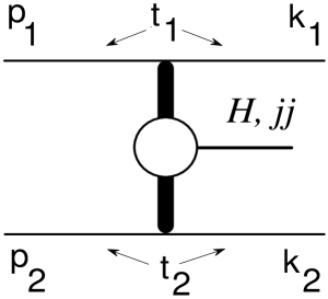
Figure 1: Production of Higgs boson $H$, dijet $jj$, by double pomeron exchange. The colliding hadrons remain intact.

2 Central inclusive dijet production

The matrix element for two gluon jet production in the Bialas-Landshoff model is given [18] by the $s$-channel discontinuity of the diagrams shown in Fig. 2.

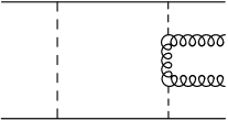
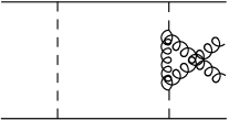
Figure 2: Three diagrams contributing to the amplitude of the process of gluon pair production by double pomeron exchange. The dashed lines represent the exchange of the non-perturbative gluons.

The square of the matrix element (averaged and summed over spins and polarizations) is of the form:

$$\overline{\left|\mathcal{M}_{pp}\right|^{2}}=81\overline{\left|\mathcal{M}_{qq}\right|^{2}}\left[F\left(t_{1}\right)F\left(t_{2}\right)\right]^{2},$$ (3)

where $\overline{\left|\mathcal{M}_{qq}\right|^{2}}$ is the production amplitude squared for colliding quarks:

$$\overline{\left|\mathcal{M}_{qq}\right|^{2}}=C\frac{s^{2}}{\left(u_{{}_{1}}\right)^{2}\left(u_{{}_{2}}\right)^{2}}\delta_{1}^{2-2\alpha(t_{1})}\delta_{2}^{2-2\alpha(t_{2})}\exp\left(2\beta\left(t_{1}+t_{2}\right)\right)R^{2}.$$ (4)

Transverse momenta of the produced gluons are denoted by $u_{{}_{1}}$ and $u_{{}_{2}}$. The constants $C$ and $R$ will be defined later. $\alpha\left(t\right)=1+\epsilon+\alpha^{\prime}t$ is the pomeron Regge trajectory with $\epsilon\approx 0.08,$ $\alpha^{\prime}=0.25$ GeV^-2 ($t_{1},$ $t_{2}$ are defined in Fig. 1). $F\left(t\right)$ = $\exp(\lambda t)$ is the nucleon form-factor with $\lambda=$ $2$ GeV^-2. $\delta_{1},$ $\delta_{2}$ are defined as $\delta_{1,2}\equiv 1-k_{1,2}/p_{1,2}$ ($k_{1},$ $k_{2},$ $p_{1},$ $p_{2},$ are defined in Fig. 1). The factor $\exp\left(2\beta\left(t_{1}+t_{2}\right)\right)$ with $\beta$ $=$ $1$ GeV^-2 [23] takes into account the effect of the momentum transfer dependence of the non-perturbative gluon propagator given by ($p^{2}$ is the Lorentz square of the momentum carried by the non-perturbative gluon):

$$D\left(p^{2}\right)=D_{0}\exp\left(p^{2}/\tau^{2}\right).$$ (5)

The constants $C$ and $R$ are defined as:

$$C =\frac{1}{\left(27\pi\right)^{2}}\left(D_{0}G^{2}\tau\right)^{6}\tau^{2}\left(\frac{g^{2}/4\pi}{G^{2}/4\pi}\right)^{2},$$ (6)

$$R =9\int d\vec{Q}_{\intercal}^{2}\text{\thinspace}\vec{Q}_{\intercal}^{2}\exp\left(-3\vec{Q}_{\intercal}^{2}\right)=1.$$ (7)

Here $G$ and $g$ are the non-perturbative and perturbative quark gluon couplings respectively. $\tau$ is the range of the non-perturbative gluon propagator (5) and $D_{0}$ its magnitude at vanishing momentum transfer. From data on the elastic scattering of hadrons one infers $D_{0}G^{2}\tau=30$ GeV^-1 and $\tau=1$ GeV.

The constant $R$ reflects the structure of the loop integral. $Q_{\intercal}$ is the transverse momentum carried by each of the three non-perturbative gluons. $R$ was shown explicitly in Eq. (4) for the reason which will become clear in the next section.

Taking into account (4) we obtain the following result for the differential cross-section [19]:

$$\frac{d\sigma}{d(E_{\intercal}^{2})d(\Delta y)dy} =R^{2}C_{E}\left(E_{\intercal}\right)^{-4}\left(\frac{s}{4E_{\intercal}^{2}\cosh^{2}(\frac{\Delta y}{2})}\right)^{2\epsilon}$$

$$\times\frac{\pi^{3}/4\alpha^{\prime}{}^{2}}{\left((\lambda+\beta)/\alpha^{\prime}-\ln\left[2E_{\intercal}\cosh(\dfrac{\Delta y}{2})/\sqrt{s}\right]\right)^{2}-y^{2}}.$$ (8)

Here $C_{E}=81C/(16\left(2\pi\right)^{8})$. $E_{\intercal}=$ $|u_{1}|=|u_{2}|$ is the transverse energy of one of the produced gluons. $\Delta y=y_{1}-y_{2},$ $y=(y_{1}+y_{2})/2$ where $y_{1,2}$ are the rapidities of the produced gluons. For completeness it is necessary to say that the rapidities $y_{1,2}$ are connected with $\delta_{1},$ $\delta_{2}$ and $E_{\intercal}$ in the following way:

$$\delta_{1}\sqrt{s}=E_{\intercal}\exp\left(y_{1}\right)+E_{\intercal}\exp\left(y_{2}\right),$$

$$\delta_{2}\sqrt{s}=E_{\intercal}\exp\left(-y_{1}\right)+E_{\intercal}\exp\left(-y_{2}\right).$$ (9)

The result (8) does not take gap survival effect ($S_{\text{gap}}^{2}$) into account $i.e.$ the probability of the gaps not to be populated by secondaries produced in the soft rescattering. From [5, 24] we expect that for the Tevatron energy it is about $0.05-0.1$. The factor $S_{\text{gap}}^{2}$ is not a universal number but it depends on the initial energy and the particular final state. Theoretical predictions of the survival factor, $S_{\text{gap}}^{2}$, can be found in Ref. [25].

The main uncertainty in the expression (8) is the value of $G^{2}/4\pi$ (see (6)). It is expected to be [26] about $1$ but in fact it should be considered only as an order of magnitude estimate.

Let us now make clear the rather $ad$ $hoc$ nature of many of the assumptions inherent in the Bialas-Landshoff approach [2]. The predictions of this model depend only weakly on energy ($\sim s^{2\epsilon}$). This is a consequence of the Regge-like dependence implied by Eq. (4). There are some controversies if such assumption is justified. In our calculations we assume the exponential form of the non-perturbative gluon propagator (5). As was already stated in [2] there is no reason to believe that the true form of $D$ is as simple as this. However, we believe that this is not a serious objection to our model. In the Bialas-Landshoff approach the produced object (Higgs, dijet $etc.$) is coupled to the non-perturbative gluons via the perturbative coupling $g$. It is not clear and the question of consistency could be addressed. Finally, let us note that estimates in the present Letter are based on the basis of the pure forward direction. It was first mentioned in [14] that such approach may lead to incorrect results.

Integrating (8) over the CDF Run I kinematical range [21] for the central inclusive production of dijets of $E_{\intercal}>7$ GeV we obtain [19] the result to be about $70$ nb (with $G^{2}/4\pi=1$ and no $S_{\text{gap}}^{2}$), to be compared with the CDF measurement of $43$ nb ($43\pm 26$ nb). We thus scale our cross section by a factor of $43/70\approx 0.6$, that is:

$$\frac{S_{\text{gap}}^{2}(\sqrt{s}=2\text{ TeV})}{\left(G^{2}/4\pi\right)^{2}}=0.6.$$ (10)

This completes the summary of [18] and [19].

3 Exclusive dijet production – Sudakov factor

As was already mentioned the calculation presented in the previous section, based on the original Bialas-Landshoff model, is a central inclusive one $i.e.$ the radiation is present in the central region of the rapidity.

In order to describe the exclusive processes one has to forbid this radiation. To do it we include the Sudakov survival factor $T(Q_{\intercal},\mu)$ inside the loop integral (7) over $Q_{\intercal}$. The Sudakov factor $T(Q_{\intercal},\mu)$ is the survival probability that a gluon with transverse momentum $Q_{\intercal}$ remains untouched in the evolution up to the hard scale $\mu=M_{gg}/2$ where $M_{gg}$ is the mass of the produced gluons. The function $T(Q_{\intercal},\mu)$ can be calculated as [5]:

$$T(Q_{\intercal},\mu)=\exp\left(-\int_{\vec{Q}_{\intercal}^{2}}^{\mu^{2}}\frac{\alpha_{s}\left(\vec{k}_{\intercal}^{2}\right)}{2\pi}\frac{d\vec{k}_{\intercal}^{2}}{\vec{k}_{\intercal}^{2}}\int_{0}^{1-\Delta}\left[zP_{gg}\left(z\right)+\sum\limits_{q}P_{qg}(z)\right]dz\right).$$ (11)

Here $\Delta=\left|k_{\intercal}\right|/\left(\mu+\left|k_{\intercal}\right|\right)$, $P_{gg}\left(z\right)$ and $P_{qg}(z)$ (we take $q=u,d,s,\bar{u},\bar{d},\bar{s}$) are the GLAP spitting functions. $\alpha_{s}$ is the strong coupling constant.

Taking into account the leading-order contributions [27] to the GLAP splitting functions:

$$P_{gg}\left(z\right) =6\left[z/(1-z)+(1-z)/z+z\left(1-z\right)+\delta\left(1-z\right)\left(11/2-n_{f}/3\right)\right],$$

$$P_{qg}\left(z\right) =\left[z^{2}+\left(1-z\right)^{2}\right]/2,$$ (12)

we obtain:

$$\int_{0}^{1-\Delta}zP_{gg}\left(z\right)dz =-11/2+12\Delta-9\Delta^{2}+4\Delta^{3}-3\Delta^{4}/2-6\ln\Delta,$$

$$\int_{0}^{1-\Delta}P_{qg}\left(z\right)dz =1/3-\Delta/2+\Delta^{2}/2-\Delta^{3}/3.$$ (13)

Now to describe the exclusive processes we use the formula (8) with $R^{2}=1$ replaced by $\tilde{R}^{2}\left(\mu\right)$ where $\tilde{R}\left(\mu\right)$ is defined as:

$$\tilde{R}\left(\mu\right)=9\int_{\Lambda^{2}}^{\mu^{2}}d\vec{Q}_{\intercal}^{2}\,\vec{Q}_{\intercal}^{2}\exp\left(-3\vec{Q}_{\intercal}^{2}\right)T\left(Q_{\intercal},\mu\right).$$ (14)

The hard scale $\mu=M_{gg}/2$ can be expressed by $E_{\intercal}$ and $\Delta y$ in the following way:

$$\mu=E_{\intercal}\cosh(\frac{\Delta y}{2}).$$ (15)

Naturally a question of internal consistency arises. Namely, the Sudakov factor uses perturbative gluons whilst in our calculations the Born amplitude (4) uses non-perturbative gluons. It is not clear what the non-perturbative gluon is and the extension of the original Bialas-Landshoff model to the exclusive processes is not straightforward. We hope that taking the Sudakov factor in the loop integral into account we obtain an approximate insight into exclusive processes. It should be emphasized that at present our calculation is a hybrid of perturbative and non-perturbative ideas.

At the end of this section let us notice that the Sudakov factor (11) does not depend on the sum of the dijet rapidities $y=\left(y_{1}+y_{2}\right)/2$. This together with the observation that $y^{2}<<\left((\lambda+\beta)/\alpha^{\prime}\right)^{2}=144$ and $4E_{\intercal}^{2}\cosh^{2}(\frac{\Delta y}{2})/s=\delta_{1}\delta_{2}$ $<<1$ leads to the conclusion that the differential cross section for DPE exclusive dijets production very weekly depends on the sum of the dijet rapidity $y$. This feature agrees with the observation found in Ref. [13]. Moreover the observed power law $E_{\intercal}^{-6.5}$ $($with $\tilde{R}^{2}\sim E_{\intercal}^{-2.2})$ is close to the observation of Ref. [7] $(\sim E_{\intercal}^{-7.3})$.

4 CDF Run I, II upper limits

The CDF collaboration has presented results on upper limits on exclusive DPE dijet production cross sections.

At Run I ($\sqrt{s}=1.8$ TeV) [21] the upper bound for exclusive dijets production was measured to be $3.7$ nb for the kinematic range of $0.035<\delta_{2}\equiv\delta_{\bar{p}}<0.095$ and jets of $E_{\intercal}>7$ GeV confined within $-4.2<y<2.4$ and the gap requirement $2.4<y_{\text{gap}}<5.9$ on the proton side.

At Run II ($\sqrt{s}=1.96$ TeV) [22] the upper bound for exclusive dijets of $E_{\intercal}>10$ GeV [$E_{\intercal}>25$ GeV] was measured to be $970$ $\pm$ $65$(stat) $\pm$ $272$(syst) pb [$34$ $\pm$ $5$(stat) $\pm$ $10$(syst) pb]. The kinematics is following: $0.03<\delta_{2}\equiv\delta_{\bar{p}}<0.1$, jets are confined within $-2.5<y<2.5$, the gap on the proton side is $3.6<y_{\text{gap}}<7.5$.

It should be noted that in the above experiments the protons were not detected and the DPE events were enhanced by a rapidity gap requirement on the proton side.

Integrating (8) over the appropriate kinematical range we obtain the results shown in Table 1. The running coupling constant $g^{2}/4\pi,$ appearing in (6), is evaluated at $2E_{\intercal}^{\min}$ $i.e.$ $0.15$, $0.14$, $0.12$ for $E_{\intercal}^{\min}=7,10,25$ GeV respectively. The factor $S_{\text{gap}}^{2}/\left(G^{2}/4\pi\right)^{2}$ is taken to be $0.6$.

$\begin{array}[c]{c}\text{Transverse}\\ \text{energy}\end{array}$	$\begin{array}[c]{c}\text{CDF}\\ \text{upper limits}\end{array}$	$\begin{array}[c]{c}\text{Model}\\ S_{\text{gap}}^{2}/\left(G^{2}/4\pi\right)^{2}=0.6\end{array}$
$E_{\intercal}>7$ GeV	$3.7$ [nb]	$1$ [nb]
$E_{\intercal}>$ $10$ GeV	$970$ $\pm$ $337$ [pb]	$300$ [pb]
$E_{\intercal}>$ $25$ GeV	$34$ $\pm$ $15$ [pb]	$3$ [pb]

Table 1: Comparison of the CDF upper limits for DPE exclusive dijet production with the results obtained in the presented model.

As can be seen from Table 1 the obtained results are quite satisfactory and encouraging. They are also comparable with those obtained in [28, 29] or [17].

5 Exclusive Higgs production

The matrix element for the Higgs production in the Bialas-Landshoff model is given [2] by the $s$-channel discontinuity of the diagram shown in Fig. 3. The Higgs coupling is taken to be through a t-quark loop.

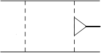
Figure 3: The diagram contributing to the amplitude of the process of Higgs boson production by double pomeron exchange. The Higgs coupling is taken to be through a t-quark loop. The dashed lines represent the exchange of the non-perturbative gluons.

The square of the matrix element for colliding (anti)protons has the form [2]:

$$\overline{\left|\mathcal{M}_{pp}\right|^{2}} =BN^{2}s^{2}\delta_{1}^{2-2\alpha(t_{1})}\delta_{2}^{2-2\alpha(t_{2})}\left[F\left(t_{1}\right)F\left(t_{2}\right)\right]^{2}$$

$$\times\exp\left(2\beta\left(t_{1}+t_{2}\right)\right)R^{2}.$$ (16)

The constant $B$ is defined as:

$$B=\frac{4\sqrt{2}}{\left(6\pi\right)^{6}}G_{F}\left(G^{2}D_{0}\tau\right)^{6}\tau^{2}\left(\frac{\alpha_{s}}{G^{2}/4\pi}\right)^{2},$$ (17)

where $G_{F}$ is the Fermi coupling constant and $\alpha_{s}(M_{H})$ is the perturbative coupling evaluated at a scale $M_{H}$. $N$ is a function of $M_{t}/M_{H}$. For the Higgs mass $M_{H}<$ $2M_{t}\approx 350$ GeV this function is given by [1]:

$$N=6\frac{M_{t}^{2}}{M_{H}^{2}}-6\frac{M_{t}^{2}}{M_{H}^{2}}\left(4\frac{M_{t}^{2}}{M_{H}^{2}}-1\right)\left(\arcsin\frac{M_{H}}{2M_{t}}\right)^{2}.$$ (18)

It turns out that the structure of the loop integral over $Q_{\intercal}$ has exactly the same form like that for gluon jets case (7). So to describe the exclusive Higgs production we take the result (16) and replace $R^{2}=1$ by $\tilde{R}^{2}\left(\mu\right)$ with $\tilde{R}\left(\mu\right)$ given by the formula (14), where $\mu=M_{gg}/2\rightarrow M_{H}/2$.

Performing the appropriate calculations we find the differential cross section $d\sigma/dy$ (not presented in [2]) for DPE exclusive Higgs boson production to be in the form:

$$\frac{d\sigma}{dy}=\frac{BN^{2}}{4^{5}\pi^{3}\alpha^{\prime}{}^{2}}\left(\frac{s}{M_{H}^{2}}\right)^{2\epsilon}\frac{\tilde{R}^{2}\left(M_{H}/2\right)}{\left((\lambda+\beta)/\alpha^{\prime}-\ln\left[M_{H}/\sqrt{s}\right]\right)^{2}-y^{2}}.$$ (19)

Here $y$, $\ln(M_{H}/\left(\delta_{2}^{\max}\sqrt{s}\right))\leqslant y\leqslant\ln(\delta_{1}^{\max}\sqrt{s}/M_{H})$, is a rapidity of the produced Higgs. In the following we use $\delta_{1}^{\max}=\delta_{2}^{\max}=\delta=0.1$. Since $y^{\max}=\ln(\delta\sqrt{s}/M_{H})$ and $(\lambda+\beta)/\alpha^{\prime}=12$ the differential cross section (19) very weekly depends on the rapidity of the Higgs. So to get the total cross section for DPE exclusive Higgs production it is enough to multiply the above result (19) (at $y=0$) by a factor $y^{\max}-y^{\min}=$ $\ln\left(s\delta^{2}/M_{H}^{2}\right)$ what leads to the final result:

$$\sigma=\frac{BN^{2}}{4^{5}\pi^{3}\alpha^{\prime}{}^{2}}\left(\frac{s}{M_{H}^{2}}\right)^{2\epsilon}\frac{\tilde{R}^{2}\left(M_{H}/2\right)}{\left((\lambda+\beta)/\alpha^{\prime}-\ln\left[M_{H}/\sqrt{s}\right]\right)^{2}}\ln\left(\frac{s\delta^{2}}{M_{H}^{2}}\right).$$ (20)

Now we are ready to give our predictions for DPE exclusive Higgs production at the Tevatron and the LHC energies. We also compare our results with those obtained in a model developed by Khoze, Martin and Ryskin (KMR model).

In Table 2 the prediction for the Tevatron energy, $\sqrt{s}=2$ TeV, is shown. The mass of the Higgs is taken to be $120$ GeV and $\alpha_{s}(M_{H})$ is about $0.1$. We also include the $\alpha_{s}$ virtual correction [5, 30] to the $gg\rightarrow H$ vertex factor, so-called $K$-factor to be about $1.5$. As was discussed earlier we take $\delta=0.1$ and assume $S_{\text{gap}}^{2}/\left(G^{2}/4\pi\right)^{2}$ to be $0.6$.

$\sqrt{s}=2$ TeV	$\begin{array}[c]{c}\text{KMR model}\\ S_{\text{gap}}^{2}=0.05\end{array}$	$\begin{array}[c]{c}\text{Our model}\\ S_{\text{gap}}^{2}/\left(G^{2}/4\pi\right)^{2}=0.6\end{array}$
$\sigma$ [fb]	$0.06$	$0.005$

Table 2: Our result for DPE exclusive Higgs production cross section for the Tevatron energy. Our prediction is about $10$ times smaller than the prediction based on the KMR model.

Before we present the prediction for the LHC energy, $\sqrt{s}=14$ TeV, we have to take into account the $s$ dependence of the gap survival factor $S_{\text{gap}}^{2}$. Following [25] we expect that $S_{\text{gap}}^{2}\left(\sqrt{s}=2\text{ TeV}\right)/S_{\text{gap}}^{2}\left(\sqrt{s}=14\text{ TeV}\right)\approx 0.4$ what allows us to assume $S_{\text{gap}}^{2}/\left(G^{2}/4\pi\right)^{2}=0.25$. The obtained result for DPE exclusive Higgs ($M_{H}=120$ GeV) production at the LHC energy is presented in Table 3.

$\sqrt{s}=14$ TeV	$\begin{array}[c]{c}\text{KMR model}\\ S_{\text{gap}}^{2}=0.02\end{array}$	$\begin{array}[c]{c}\text{Our model}\\ S_{\text{gap}}^{2}/\left(G^{2}/4\pi\right)^{2}=0.25\end{array}$
$\sigma$ [fb]	$2$	$0.015$

Table 3: Our result for DPE exclusive Higgs production cross section for the LHC energy. A distinct difference, $\sim 10^{2}$, with the KMR model prediction is observed.

As can be seen from Table 2 and Table 3 the results for DPE exclusive Higgs production are about one order of magnitude smaller than those obtained in the KMR model [5, 6] for the Tevatron energy and about two orders of magnitude smaller for the LHC energy. It reflects the possible large uncertainties of the presented approach and the general fact that the perturbative QCD predictions, on the contrary to the non-perturbative two-gluon-exchange-type models, show a strong increase of the cross sections with increasing energy. Hopefully a study of the dijets production as a function of the energy will clearly be able to discriminate between the perturbative QCD determinations and the non-perturbative model approaches.

Acknowledgements It is a pleasure to thank Dr. Leszek Motyka, Prof. Andrzej Bialas and Prof. Robert Peschanski for useful discussions. This investigation was supported by the Polish State Committee for Scientific Research (KBN) under grant 2 P03B 043 24.

References

• [1] A. Schafer, O. Nachtmann, R. Schopf, Phys. Lett. B249 (1990) 331.
• [2] A. Bialas, P.V. Landshoff, Phys. Lett. B256 (1991) 540.
• [3] J.R. Cudell, O.F. Hernandez, Nucl. Phys. B471 (1996) 471.
• [4] D. Kharzeev, E. Levin, Phys. Rev. D63 (2001) 073004.
• [5] V.A. Khoze, A.D. Martin, M.G. Ryskin, Eur. Phys. J. C14 (2000) 525.
• [6] V.A. Khoze, A.D. Martin, M.G. Ryskin, Eur. Phys. J. C19 (2001) 477, erratum C20 (2001) 599.
• [7] A.B. Kaidalov, V.A. Khoze, A.D. Martin, M.G. Ryskin, Eur. Phys. J. C33 (2004) 261.
• [8] B. Cox, J. Forshaw, B. Heinemann, Phys. Lett. B540 (2002) 263.
• [9] M. Boonekamp, R. Peschanski, C. Royon, Phys. Rev. Lett. 87 (2001) 251806.
• [10] M. Boonekamp, A. De Roeck, R. Peschanski, C. Royon, Acta Phys. Polon. B33 (2002) 3485; M. Boonekamp, R. Peschanski, C. Royon, Nucl. Phys. B669 (2003) 277; M. Boonekamp, R. Peschanski, C. Royon, Phys. Lett. B598 (2004) 243.
• [11] N. Timneanu, R. Enberg, G. Ingelman, Acta Phys. Polon. B33 (2002) 3479; R. Enberg, G. Ingelman, A. Kissavos, N. Timneanu, Phys. Rev. Lett. 89 (2002) 081801; R. Enberg, G. Ingelman, N. Timneanu, Phys. Rev. D67 (2003) 011301.
• [12] A. Berera, J. Collins, Nucl. Phys. B474 (1996) 183; A. Berera, Phys. Rev. D62 (2000) 014015.
• [13] A.D. Martin, M.G. Ryskin, V.A. Khoze, Phys. Rev. D56 (1997) 5867.
• [14] J. Pumplin, Phys. Rev. D52 (1995) 1477.
• [15] A. Bialas, W. Szeremeta, Phys. Lett. B296 (1992) 191; W. Szeremeta, Acta Phys. Polon. B24 (1993) 1159. A. Bialas, R. Janik, Z. Phys. C62 (1994) 487.
• [16] R. B. Appleby, J. R. Forshaw, Phys. Lett. B541 (2002 ) 108.
• [17] R.J.M. Covolan, M.S. Soares, Phys. Rev. D67 (2003) 077504.
• [18] A. Bzdak, Acta Phys. Polon. B35 (2004) 1733.
• [19] A. Bzdak, Phys. Lett. B608 (2005) 64.
• [20] P.V. Landshoff, O. Nachtmann, Z. Phys. C35 (1987) 405; A. Donnachie, P.V. Landshoff, Nucl. Phys. B311 (1988) 509.
• [21] T. Affolder et al. (CDF Collaboration), Phys. Rev. Lett. 85 (2000) 4215.
• [22] K. Goulianos, AIP Conf. Proc. 698 (2004) 110; M. Gallinaro, Acta Phys. Polon. B35 (2004) 465.
• [23] A. Donnachie, P. V. Landshoff, Nucl. Phys. B267 (1986) 690.
• [24] T. Affolder et al. (CDF Collaboration), Phys. Rev. Lett. 84 (2000) 5043.
• [25] V.A. Khoze, A.D. Martin, M.G. Ryskin, Eur. Phys. J. C18 (2000) 167; A.B. Kaidalov, V.A. Khoze, A.D. Martin, M.G. Ryskin, Eur. Phys. J. C21 (2001) 521.
• [26] J.R. Cudell, A. Donnachie, P.V. Landshoff, Nucl. Phys. B322 (1989) 55.
• [27] G. Altarelli, G. Parisi, Nucl. Phys. B126 (1977) 298.
• [28] V.A. Khoze, A.D. Martin, M.G. Ryskin, hep-ph/0006005, in Proc. of $\mathit{8}$th Int. Workshop on Deep Inelastic Scattering and QCD (DIS$\mathit{2000}$), Liverpool, eds. J. Gracey and T. Greenshaw (World Scientific, 2001), p. 592.
• [29] V.A. Khoze, A.D. Martin, M.G. Ryskin, W.J. Stirling, Eur. Phys. J. C38 (2005) 475.
• [30] M. Spira et al., Nucl. Phys. B453 (1995) 17.