Abstract

While the Quasi-Monte Carlo method of numerical integration achieves smaller integration error than standard Monte Carlo, its use in particle physics phenomenology has been hindered by the abscence of a reliable way to estimate that error. The standard Monte Carlo error estimator relies on the assumption that the points are generated independently of each other and, therefore, fails to account for the error improvement advertised by the Quasi-Monte Carlo method. We advocate the construction of an estimator of stochastic nature, based on the ensemble of pointsets with a particular discrepancy value. We investigate the consequences of this choice and give some first empirical results on the suggested estimators.

1 Monte Carlo and Quasi-Monte Carlo

1.1 Introduction

In numerical integration, the main problem is not to obtain a numerical answer for the integral, but rather, on the one hand, to ensure that the inherent numerical error is as small as possible, and, on the other hand, to estimate this error as precisely as possible. For integrands with well-known smoothness properties, a-priori estimates of the numerical error are possible, but for most practical applications the smoothness properties of the integrand can only be investigated in the course of the integration itself, that is, by repeated numerical evaluation of the integrand.

In this paper, we shall be concerned with the integration errors arising in Monte Carlo and Quasi-Monte Carlo integration. In these methods, the integration nodes are distributed in a (more or less) stochastic manner, and the integration errors are therefore of an essentially probabilistic nature. The difference between Monte Carlo and Quasi-Monte Carlo is that in the former, the integration points are iid uniform in the integration region, while in the latter the integration points are not chosen independently, but rather with an explicit interdependence so that their overall distribution is ‘smoother’, in a sense discussed below.

In stochastic integration methods of the Monte Carlo or Quasi-Monte Carlo types, the integration error is itself an estimate, which contains its own error. That this is not an academic point becomes clear when we realize that the error estimate is routinely used to provide confidence levels for the integral estimate (be it based either on Chebyshev or Central-Limit-Theorem, Gaussian rules); and a mis-estimate of the integration error can lead to a serious under- or overestimate of the confidence level. As an example, suppose that the Central Limit Theorem is applicable, so that the integration result is drawn from a Gaussian distribution centered around the true integral value. One standard deviation, as estimated by Monte Carlo, corresponds to a two-sided confidence level of 68%. If the error estimate is off by 50% (admittedly a large value), the actual confidence level may then be anything between 38% and 87%.

From this consideration, we are therefore led to a hierarchy of error estimates: the first-order error is that on the integral estimate, while the second-order error is the error on the error estimate. This in turn has, of course, its own third-order error, and so on. Higher orders than the second one, however, appear to be too academic for practical relevance, but we should like to argue that, in any serious integration problem, the second-order error ought to be included. In what follows we shall discuss the first- and second-order error estimates.

Due to the absence of a Quasi-Monte Carlo error estimator, users of Quasi-Monte Carlo have been estimating the integration error with the classical Monte Carlo formula, as if the point set was iid. This systematically overestimates the error in any case where the quasi point-set is of any worth. Moreover, no confidence levels can be assigned since the classical estimator does not average to the error made by the quasi, non-iid point-sequence. The purpose of this paper is to investigate possible estimators for Quasi-Monte Carlo integration taking under consideration the non-iid nature of the underlying point-set.

1.2 Monte Carlo estimators

In this section we briefly review the probabilistic theory underlying Monte Carlo integration. This is of course well known, but we include it here so that the significant difference with Quasi-Monte Carlo can become clear.

Throughout this paper we shall consider integration problems over the $d$-dimensional unit hypercube $C=[0,1)^{d}$. The integrand is a function $f(\vec{x})$, which we shall assume real and non-negative, and, of course, integrable over $C$. We shall define

$$J_{m}=\int\limits_{C}\;f(\vec{x})^{m}\;d^{d}\vec{x}\;\;\;,\;\;\;m=1,2,3,\ldots\;\;,$$ (1)

so that $J_{1}$ is the required integral. Note that $J_{m}$ is not necessarily finite for $m\geq 2$. In Monte Carlo we assume $N$ integration points, to be chosen iid from the uniform probability distribution over $C$. This means that the point set $X=\{\vec{x}_{1},\vec{x}_{2},\ldots,\vec{x}_{N}\}$ on which the integration is based is assumed to be a typical member of an ensemble of such point sets, in such a way that the combined probability distribution of the $N$ points over this ensemble is the uniform iid one:

$$P_{N}(\vec{x}_{1},\vec{x}_{2},\ldots,\vec{x}_{N})=1\;\;.$$ (2)

We shall take the averages over this ensemble. Other assumptions on the underlying ensemble from which the point set $X$ is believed to be chosen are possible, leading to a different form of $P_{N}$. In this, the situation is not different from that encountered in statistical mechanics. The above assumption, however, is the one that is always made in regular Monte Carlo  and is justified to some extent by the fact that good-quality (pseudo)random number generators are actually available, allowing us to build ensembles of point sets $X$ that indeed have the above property (2).

Let us assume that a point set $X$ has been generated, and the values of the integrand $f(\vec{x})$ at all these points have been computed. These we shall denote by $f_{j}\equiv f(\vec{x}_{j})$, $j=1,2,\ldots,N$. From these we can compute the discrete analogues of the integrals $J_{m}$, which are computable in linear time (that is, time proportional to $N$):

$$S_{m}=\sum\limits_{j=1}^{N}\;(f_{j})^{m}\;\;.$$ (3)

The Monte Carlo estimate of the integral is then

$$E_{1}={1\over N}S_{1}\;\;.$$ (4)

The expected value of $E_{1}$ over the above ensemble of point sets is given by

$$\left\langle E_{1}\right\rangle={1\over N}\sum\limits_{i}\left\langle f_{i}\right\rangle=\int\limits_{C}f(\vec{x})\;d^{d}\vec{x}=J_{1}\;\;,$$ (5)

which is indeed the required integral: this is the basis for the Monte Carlo method. Its usefulness appears if we compute the variance of $E_{1}$:

$$\sigma\left(E_{1}\right)^{2}=\left\langle E_{1}^{2}\right\rangle-\left\langle E_{1}\right\rangle^{2}={1\over N}\left(J_{2}-J_{1}^{2}\right)\;\;.$$ (6)

Since this decreases as $N^{-1}$, the Monte Carlo method actually converges for large $N$. Note that the leading, ${\cal O}(N^{0})$, terms of $\langle E_{1}^{2}\rangle$ and $\langle E_{1}\rangle^{2}$ cancel against each other: this is a regular phenomenon in variance estimates of this kind. The variance $\sigma\left(E_{1}\right)^{2}$ is estimated by the first-order error estimator (also called ‘classical’ or ‘pseudo’ estimator in what follows)

$$E_{2}={1\over N^{2}}S_{2}-{1\over N^{3}}S_{1}^{2}\;\;,$$ (7)

for which we have

$$\left\langle E_{2}\right\rangle=\sigma\left(E_{1}\right)^{2}+{\cal O}(N^{-2})\;\;.$$ (8)

Since $N$ is usually quite large, at least 10,000 or so, we feel justified in working only to leading order in $N$. The squared error of $E_{2}$ is computed to be, to leading order in $N$,

$$\sigma\left(E_{2}\right)^{2}={1\over N^{3}}\left(J_{4}-4J_{3}J_{1}-J_{2}^{2}+8J_{2}J_{1}^{2}-4J_{1}^{4}\right)\;\;,$$ (9)

for which the estimator is

$$E_{4} = {1\over N^{7}}\left(N^{3}S_{4}-4N^{2}S_{3}S_{1}-N^{2}S_{2}^{2}+8NS_{2}S_{1}^{2}-4S_{1}^{4}\right)\;\;.$$ (10)

which can also be computed in linear time; we have

$$\left\langle E_{4}\right\rangle=\sigma\left(E_{2}\right)^{2}+{\cal O}(N^{-4})\;\;.$$ (11)

Some details on the computation of leading-order expectation values of this type, as well as (for purposes of illustration) the form of the third- and fourth-order error estimators, $E_{8}$ and $E_{16}$, respectively, are given in the Appendix.

A final remark is in order here. The Central Limit theorem, which ensures that the error estimate can be used to derive Gaussian confidence levels, can also be inferred from the computation of the higher cumulants of the error distribution: we find for the skewness

$$\left\langle\left(E_{1}-\left\langle E_{1}\right\rangle\right)^{3}\right\rangle={1\over N^{2}}\left(J_{3}-3J_{2}J_{1}+2J_{1}^{3}\right)\;\;,$$ (12)

and the unnormalized kurtosis:

$$\left\langle\left(E_{1}-\left\langle E_{1}\right\rangle\right)^{4}\right\rangle-3\sigma\left(E_{1}\right)^{2}={1\over N^{3}}\left(J_{4}-4J_{3}J_{1}-3J_{2}^{2}+12J_{2}J_{1}^{2}-6J_{1}^{4}\right)\;\;,$$ (13)

which indicate that the higher cumulants decrease faster than the variance with increasing $N$; we shall examine this later on for the case of Quasi-Monte Carlo.

1.3 Quasi-Monte Carlo estimators

1.3.1 Multi-point distribution and correlation functions

In contrast to the case of regular Monte Carlo, the technique of Quasi-Monte Carlo relies on point sets in which the points are not chosen iid from the uniform distribution, but rather interdependently. To make this more specific, let us consider a point set $X$ of $N$ points. For each such a point set, we may define a measure of non-uniformity, called a discrepancy or, as in this paper, a diaphony. Its precise definition is presented below: for now, suffice it to demand that there exist a function $D(X)$ of the point set, which increases with its non-uniformity: $D(X)=0$ if the point set is perfectly uniform in all possible respects, an ideal situation that can never be obtained for any finite point set. The Quasi-Monte Carlo method consists of using point sets $X$ for which $D(X)$ has some value $s$ which is (very much) smaller than $\left\langle s\right\rangle$, the value that may be expected for truly iid uniform ones.

Given that such ‘quasi-random’ point sets can be obtained, how does one use them in numerical integration? The obvious issue here is to determine of what ensemble the quasi-random point set $X$ can be considered to be a ‘typical’ member. In this paper, we should like to advocate the viewpoint that, since the main additional property of the quasi-random point set that distinguishes it from truly random point sets is its ‘anomalously small’ discrepancy $D$, the ensemble ought to consist of those point sets that are iid uniformly, with the additional constraint that the discrepancy $D$ has the particular value $D(X)=s$ for the actually used point set. On this premise, the Quasi-Monte Carlo analogue of Eq.(2) would then be the assumption

$$P_{N}(s;\vec{x}_{1},\vec{x}_{2},\ldots,\vec{x}_{N})={1\over H(s)}\delta(D(X)-s)\;\;,$$ (14)

where $s$ is, again, the observed value of the discrepancy of $X$, on which $P_{N}$ must now of course depend; and $H(s)$ is the probability density to happen upon a point sets $X$ with this discrepancy in the regular-Monte Carlo ensemble:

$$H(s)=\int\limits_{C}\;\delta(D(X)-s)\;d^{d}\vec{x}_{1}\;d^{d}\vec{x}_{2}\;d^{d}\vec{x}_{N}\\$$

The actual computation of $H(s)$ for given definition of the discrepancy is referred to the next section. What interests us here is the fact that $P_{N}$ is now no longer simply unity, since that would imply independence of the points in the point set. Let us therefore write the multi-pont distribution as

$$P_{N}(s;\vec{x}_{1},\vec{x}_{2},\ldots,\vec{x}_{N})=1-{1\over N}F_{2}(s;\vec{x}_{1},\vec{x}_{2},\ldots,\vec{x}_{N})\;\;,$$ (15)

where we have anticipated a factor $1/N$ in the multi-point correlation $F$.

1.3.2 Properties of the correlation function

Since the value of the discrepancy of a given point-set $X$, should be independent of the order in which the points are generated, $F_{k}(s;\vec{x}_{1}\ldots\vec{x}_{k})$ must be totally symmetric; moreover, we must have

$$F_{k}(s;\vec{x}_{1},\vec{x}_{2},\ldots,\vec{x}_{K})=\int\limits_{C}\;F_{k+1}(s;\vec{x}_{1},\vec{x}_{2},\ldots,\vec{x}_{k},\vec{x}_{k+1})\;d^{d}\vec{x}_{k+1}\;\;,$$ (16)

which is not as trivial as it might seem since the value of the discrepancy, $s$, is based on the full $N$ points and not on the smaller set of $k$ or $k+1$ points. Finally, for the Quasi-Monte Carlo integral to be unbiased, we must have

$$P_{1}(s;\vec{x}_{1})=1\;\;,$$ (17)

so that

$$\int\limits_{C}\;F_{2}(s;\vec{x}_{1},\vec{x}_{2})\;d^{d}\vec{x}_{2}=0\;\;.$$ (18)

These remain, of course, to be proven and we shall do so in the next section, for a particular choice of discrepancy. Moreover, we shall show there that the multi-point correlation $F_{N}$ is, to leading order in $1/N$, made up from two-point correlations $F_{2}$:

$$F_{k}(s;\vec{x}_{1},\vec{x}_{2},\ldots,\vec{x}_{k})=\sum\limits_{1\leq m<n\leq k}F_{2}(s;\vec{x}_{m},\vec{x}_{n})\;\;.$$ (19)

This establishes the properties of our ensemble of point sets $X$ on which, in our view, the Quasi-Monte Carlo estimates ought to be based.

1.3.3 Estimators

We shall indicate the ‘Quasi-Monte Carlo’ nature of the estimators by the superscript $(q)$. The first estimator is that of the integral:

$$E_{1}^{(q)}={1\over N}\sum f_{j}\;\;.$$ (20)

Here, and in the rest of this section, the sums will run from 1 to $N$. Denoting by the subscript $(q)$ averages with respect to the ‘quasi-random’ ensemble discussed above, we then have

$$\left\langle E_{1}^{(q)}\right\rangle_{(q)}=\int\limits_{C}\;f(\vec{x})\;P_{1}(s;\vec{x})\;d^{d}\vec{x}=J_{1}\;\;,$$ (21)

as before: owing to the fact that the one-point distribution is uniform, the Quasi-Monte Carlo estimate is indeed as unbiased as the Monte Carlo one. The distinction between the two methods appears in the first-order error estimate. Let us define

$$\alpha(\vec{x}_{i},\vec{x}_{j})=1+F_{2}(s;\vec{x}_{i},\vec{x}_{j})\;\;;$$ (22)

then, we have

$$\sigma\left(E_{1}^{(q)}\right)^{2}_{(q)}={1\over N}\left(J_{2}-\int f_{1}f_{2}\alpha_{12}\right)\;\;\;+\;\;\;{\cal O}\left({1\over N^{2}}\right)\;\;.$$ (23)

where we have adopted the straightforward convention for integrals

$$\int f_{1}f_{2}\alpha_{12}=\int\limits_{C}\;f(\vec{x}_{1})\;f(\vec{x}_{2})\;\alpha(\vec{x}_{1},\vec{x}_{2})\;d^{d}\vec{x}_{1}\;d^{d}\vec{x}_{2}\;\;,$$ (24)

etcetera. As before, we shall insouciantly neglect terms that are sub-leading in $1/N$. The advantage of the Quasi-Monte Carlo method is now clear: if we can ensure that $\alpha_{12}>1$ ‘where it counts’, that is, generally, when $\vec{x}_{1}$ and $\vec{x}_{2}$ are ‘close’ in some sense, then the Quasi-Monte Carlo error will be smaller than the Monte Carlo one. A good Quasi-Monte Carlo point set, therefore, is one in which the points ‘repel’ each other to some extent.

The first-order error estimate is now simply

$$E_{2}^{(q)}={1\over N^{2}}\sum f_{i}^{2}-{1\over N^{3}}\sum\limits f_{i}f_{j}\alpha_{ij}\;\;.$$ (25)

It is simple to show that, indeed

$$\left\langle E_{2}^{(q)}\right\rangle_{(q)}=\sigma\left(E_{1}^{(q)}\right)^{2}_{(q)}+{\cal O}(N^{-2})\;\;;$$ (26)

however, evaluating $E_{2}^{(q)}$ is less trivial since it is not obvious how to do this in time linear in $N$. We shall discuss this later. The variance of the estimator $E_{2}^{(q)}$ can be evaluated to

$$\sigma\left(E_{2}^{(q)}\right)^{2} = {1\over N^{3}}\left(\int f_{i}^{4}-4\int f_{i}^{3}f_{j}\alpha_{ij}-\int f_{i}^{2}f_{j}^{2}\alpha_{ij}\right.$$ (27)

$$+4\int f_{i}^{2}f_{k}f_{l}\alpha_{ik}\alpha_{kl}+4\int f_{i}^{2}f_{k}f_{l}\alpha_{ik}\alpha_{il}$$

$$\left.-4\int f_{i}f_{j}f_{k}f_{l}\alpha_{ij}\alpha_{jk}\alpha_{kl}\right)+{\cal O}(N^{-4})\;\;,$$

for which the corresponding estimator (to leading order) is

$$E_{4}^{(q)} = {1\over N^{7}}\left(N^{3}\sum f_{i}^{4}-4N^{2}\sum f_{i}^{3}f_{j}\alpha_{ij}-N^{2}\sum f_{i}^{2}f_{j}^{2}\alpha_{ij}\right.$$ (28)

$$+4N\sum f_{i}^{2}f_{k}f_{l}\alpha_{ik}\alpha_{kl}+4N\sum f_{i}^{2}f_{k}f_{l}\alpha_{ik}\alpha_{il}$$

$$\left.-4\sum f_{i}f_{j}f_{k}f_{l}\alpha_{ij}\alpha_{jk}\alpha_{kl}\right)\;\;.$$

The details of this computation are discussed in the Appendix. It goes without saying that the substitution $\alpha_{ij}\to 1$ will reduce all the Quasi-Monte Carlo results to the regular Monte Carlo ones.

We can now see why the ‘classical’ estimator Eq.(7) overestimates the error. Under the quasi distribution $P_{2}$ of Eq.(15) the classical estimator averages to

$$\left\langle E_{2}\right\rangle_{(q)} = \left\langle{1\over N^{2}}\sum_{i}f_{i}^{2}-{1\over N^{3}}\sum_{i,j}f_{i}f_{j}\right\rangle_{(q)}$$ (29)

$$= {1\over N}(J_{2}-J_{1}^{2})-{1\over N^{2}}\int{f(x)f(y)F(x,y)}+{\cal O}(\frac{1}{N^{2}})$$

The term involving the correlator is suppressed by ${1\over N}$, which shows that $E_{2}$ averages to something different than the variance of $E_{1}$ under the quasi distribution. Moreover, we will show in section 2.3 that the integral of the suppressed term is strictly positive for any point-set that is better than a truly random one. So $E_{2}$ omits a strictly negative term when estimating the error.

While it is true that the estimator Eq.(25) averages to a quantity whose leading order in $N$ is equal to the leading order of $\sigma\left(E_{2}^{(q)}\right)^{2}$, it suffers from the following disagreeable property: for a constant integrand, while the first two terms vanish identically, the third approaches zero asymptotically from negative values. This leads to a negative squared error for all practical purposes. Although this is not disastrous per se, it indicates the reason for the appearance of negative errors also for non-constant integrands, as will become apparent once we have a concrete expression for the correlation function. It is, thus, desirable to obtain an estimator that vanishes identically for constant functions. This is achieved by

$$E_{2}^{(q_{2})}={1\over{N}^{\underline{2}}}\sum_{i}f_{i}^{2}-{1\over N{N}^{\underline{2}}}\hat{\sum_{i,j}}f_{i}f_{j}-{1\over N{N}^{\underline{4}}}\hat{\sum_{i,j,k,l}}f_{i}f_{j}(F_{i,j}-F_{i,k}-F_{l,j}+F_{l,k})$$ (30)

where the $\hat{\Sigma}_{i,j\ldots}$ denotes a sum with all indices different, and $F_{i,j}\equiv F_{2}(s;\vec{x}_{i},\vec{x}_{j})$. This quantity averages to

$$\left\langle E_{2}^{(q_{2})}\right\rangle={1\over N}(J_{2}-J_{1}^{2})-{1\over N}\int dxdydzdw\;f(x)f(y)\left[F_{x,y}-F_{x,w}-F_{z,y}+F_{z,w}\right]$$ (31)

which equals the leading part of $\sigma\left(E_{2}^{(q)}\right)^{2}$ thanks to Eq.(18). It is easy to check that the estimator of Eq.(30) vanishes identically for a constant integrand and any $N$, thanks to the antisymmetry property of the quadruple sum.

1.3.4 Cumulants of $E_{1}$

As a final remark, we may also investigate the cumulants of the Quasi-Monte Carlo estimator $E_{1}$. We write the expansion of the correlation function $F_{k}$ over $1/N$ as

$$F_{k}(s;\vec{x}_{1},\ldots,\vec{x}_{k})\equiv F_{k}^{(1)}+\frac{1}{N}F_{k}^{(2)}+\frac{1}{N^{2}}F_{k}^{(3)}+\ldots$$ (32)

and define

$$\mathcal{M}_{i_{1},\ldots,i_{k}}^{(a)}\equiv\int f(\vec{x}_{1})^{i_{1}}\ldots f(\vec{x}_{k})^{i_{k}}F_{k}^{(a)}(s;\vec{x}_{1},\ldots,\vec{x}_{k})$$ (33)

It is evident that if Eq.(19) holds, we have

$$\mathcal{M}_{1,1,\ldots,1}^{(1)}=\frac{{k}^{\underline{2}}}{2}J_{1}^{k-2}\mathcal{M}_{1,1}^{(1)}$$ (34)

The cumulants are defined as

$$c_{n}=\left\langle\left(E_{1}^{(q)}-\left\langle E_{1}^{(q)}\right\rangle_{(q)}\right)^{n}\right\rangle_{(q)}$$ (35)

The variance of $E_{1}$ is then

$$c_{2}=\frac{1}{N}(J_{2}-J_{1}^{2}-\mathcal{M}_{1,1}^{(1)})+O(\frac{1}{N^{2}})$$ (36)

The skewness is

$$c_{3}=\frac{1}{N^{2}}(J_{3}-3J_{1}J_{2}+2J_{1}^{3}-3\mathcal{M}_{1,2}^{(1)}+3J_{1}\mathcal{M}_{1,1}^{(2)}+6J_{1}\mathcal{M}_{1,1}^{(1)}-\mathcal{M}_{1,1,1}^{(2)})+O(\frac{1}{N^{3}})$$ (37)

The unnormalized kurtosis is

$$c_{4}-3c_{2}^{2}=\frac{1}{N^{2}}(-\mathcal{M}_{1,1,1,1}^{(2)}-3(\mathcal{M}_{1,1}^{(1)})^{2}+4J_{1}\mathcal{M}_{1,1,1}^{(2)}-6J_{1}^{2}\mathcal{M}_{1,1}^{(2)})+O(\frac{1}{N^{3}})$$ (38)

The above results indicate that a correlation function that satisfies the property of Eq.(19) leads to a distribution whose skewness decreases faster with $N$ than does the variance, but when it comes to the kurtosis (and higher cumulants), additional properties regarding the next-to-leading order expression for $F$ (denoted above by $\mathcal{M}_{i_{1},\ldots,i_{k}}^{(2)}$) are needed to secure Gaussian cumulants. These properties hold whenever the saddle point approximation of Eq.(65-66) is valid. In such cases one expects Gaussian confidence levels for the Quasi-Monte Carlo estimator $E_{1}$.

2 Multi-point distributions with diaphonies

2.1 Diaphony

We consider a point set $X$ with $N$ elements, given in $C$. The non-uniformity of the point set $X$ can be described by its diaphony:

$$D(X)={1\over N}\sum\limits_{j,k=1}^{N}\beta(\vec{x}_{j},\vec{x}_{k})\;\;,$$ (39)

with

$$\beta(\vec{x}_{j},\vec{x}_{k}) = \hat{\sum\limits_{\vec{n}}}\;\sigma^{2}_{\vec{n}}\;e_{\vec{n}}(\vec{x}_{j})\bar{e}_{\vec{n}}(\vec{x}_{k})\;\;,$$

$$e_{\vec{n}}(\vec{x}) = \exp(2i\pi\;\vec{n}\cdot\vec{x})\;\;.$$ (40)

Here, the vectors $\vec{n}=(n_{1},n_{2},\ldots,n_{d})$ form the integer lattice, and the hat denotes the sum over all $\vec{n}$ except $\vec{n}=\vec{0}$. We may also write

$$D(X)={1\over N}\hat{\sum\limits_{\vec{n}}}\sigma^{2}_{\vec{n}}\;\left|\sum\limits_{j=1}^{N}e_{\vec{n}}(\vec{x}_{j})\right|^{2}\;\;,$$ (41)

so that we recognize the diaphony as a measure of how well the various Fourier modes are integrated by the point set $X$. The diaphony is therefore seen to be related to the ‘spectral test’, well-known in the field of random-number generator testing. For the mode strengths $\sigma^{2}_{\vec{n}}$ we have

$$\sigma^{2}_{\vec{n}}\geq 0\;\;\;,\;\;\;\hat{\sum\limits_{\vec{n}}}\sigma^{2}_{\vec{n}}=1\;\;.$$ (42)

The latter convention simply establishes the overall normalization of $D$. The advantage of this diaphony over, say, the usual (star)discrepancy is the fact that it is translation-invariant:

$$\beta(\vec{x}_{j},\vec{x}_{k})=\beta(\vec{x}_{j}-\vec{x}_{k})\;\;,$$ (43)

so that point sets $X$ and $X^{\prime}$ that differ only by a translation (modulo 1) have the same non-uniformity: the diaphony is actually defined on the hyper-torus rather than on the hypercube. Also, the diaphony is tadpole-free:

$$\int\limits_{C}\;\beta(\vec{x})\;d^{d}\vec{x}=0\;\;.$$ (44)

Moreover, we shall use $\sigma^{2}_{\vec{n}}$ such that $\sigma^{2}_{\vec{n}}=\sigma^{2}_{\vec{n}^{\prime}}$ if the two lattice vectors $\vec{n}$ and $\vec{n}^{\prime}$ differ only by a permutation of their components. Thus, $X$ and $X^{\prime}$ will also have the same non-uniformity if they differ by a global permutation of the coordinates of the points.

2.1.1 Some numerical results

In this section the behavior of a specific diaphony is presented, for three point sequences, as the number of points $N$ increases.

The diaphony is defined by Eq.(41) with

$$\sigma_{\vec{n}}=Ke^{-\lambda\vec{n}^{2}}\;\;\;\;K^{-1}=\sum e^{-\lambda\vec{n}^{2}}\;\;\;\lambda=0.1$$ (45)

The reason for experimenting with this definition lies in the factorizing property of the $\sigma_{\vec{n}}$. Due to $K^{-1}$ being related to Jacobi theta functions, we call this the ‘Jacobi diaphony’. We will be using this diaphony in most of what follows.

In this paper we will be using three point sequences that we will be calling Ranlux, Van Der Corput and Niederreiter. Ranlux is a pseudo-random point sequence generated by the Ranlux algorithm (see [4]) with luxury level equal to $3$. Van Der Corput is a quasi-random sequence generated by an implementation of the algorithm by Halton that generalizes to many dimensions an older algorithm by Van der Corput (see [5]) with prime bases $2,3,5,7,11,\ldots$. Finally Niederreiter is another, optimal quasi-random sequence based on the algorithm in (see [7]). In particular, we follow the choices of [8] and construct the sequence in whichever base is optimal for the current dimension (see [7]).

It should also be noted that only modes with square length up to $\vec{n}^{2}\leq 15$ are included in the calculation of the diaphony (including the determination of $K$), in anticipation of the same restriction on the estimator sums in later sections.

In the plots that follow, the diaphony of the Niederreiter sequence in particular, but also that of the van der Corput sequence, exhibited a large variation in relatively small intervals of $N$. As the number of points $N$ approaches certain critical values the diaphony reaches very small levels, only to return to its ‘cruising’ values a few points later. To avoid cluttering the plots we present here the diaphony averaged in packs of $500$ points without information on the minimum or maximum value found in each pack. The minimum values for each pack, that correspond to exceptional point configurations, are very interesting on their own but do not affect the present study.

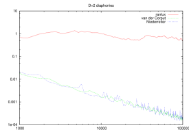
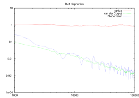
Figure 1: D=2 (left) and D=3 (right). The diaphony of RANLUX (red line), Van Der Corput (green line) and Niederreiter (blue line).

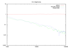
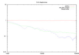
Figure 2: D=4 (left) and D=5 (right). The diaphony of RANLUX (red line), Van Der Corput (green line) and Niederreiter (blue line).

The diaphony of the RANLUX sequence is seen to oscillate around 1, as expected. Moreover the behavior of the Niederreiter sequence improves with the number of dimensions when compared with crude Van der Corput, an encouraging hint for higher dimensions.

2.2 Generating function

We shall now compute a $1/N$ approximation to the moment-generating distribution of the $p$-point probability distribution, that is,

$$G_{p}(z)=\left\langle\exp(zD(X))\vphantom{A^{A}}\right\rangle_{\vec{x}_{p+1},\vec{x}_{p+2},\ldots,\vec{x}_{N}}\;\;,$$ (46)

where we have indicated that the points $\vec{x}_{1},\vec{x}_{2},\ldots,\vec{x}_{p}$ are kept fixed while the remaining $N-p$ points are integrated over. $G_{p}(z)$ therefore still depends on $\vec{x}_{1},\ldots,\vec{x}_{p}$. This is most easily achieved using a diagrammatic approach, which has been introduced in [2]. We shall indicate with crosses those points that are kept fixed (with an implied sum over them, from 1 to $p$), and with dots (‘beads’) those points that are integrated over (again, with an implied sum running from $p+1$ to $N$). The function $\beta$ is indicated by a solid line. As the simplest examples, then, we have

$$\mbox{if $p=N$:}\;\;\;{1\over N}\raisebox{-1.42271pt}{\psfig{width=42.67912pt}}={1\over N}\sum\limits_{j,k=1}^{N}\beta(\vec{x}_{j}-\vec{x}_{k})=D(X)\;\;,$$ (47)

and

$$\mbox{if $p=0$:}\;\;\;\langle D(X)\rangle_{\vec{x}_{1},\ldots,\vec{x}_{N}}=\beta(0)=\raisebox{-8.5359pt}{\psfig{width=17.07182pt}}=1\;\;.$$ (48)

Other examples are

$$= \int\limits_{C}\;\beta(\vec{x}_{1}-\vec{x}_{2})^{2}\;d^{d}\vec{x}_{1}\;d^{d}\vec{x}_{2}\;\;,$$

$$= \int\limits_{C}\;\beta(\vec{x}_{1}-\vec{x}_{2})\beta(\vec{x}_{2}-\vec{x}_{3})\beta(\vec{x}_{3}-\vec{x}_{1})\;d^{d}\vec{x}_{1}\;d^{d}\vec{x}_{2}\;d^{d}\vec{x}_{3}\;\;,$$ (49)

and so on: a general closed loop with precisely $n$ beads will be denoted by . Note that, since, the functions $e_{\vec{n}}(\vec{x})$ form an orthonormal (and even a complete) set, we have

$$\raisebox{-8.5359pt}{\psfig{width=19.91684pt}}=\hat{\sum\limits_{\vec{n}}}\left(\sigma^{2}_{\vec{n}}\right)^{n}\;\;.$$ (50)

We can now simply write out all possible (connected and disconnected) diagrams where every solid line ends in a cross or a bead, and apply the following Feynman rules:

1. A factor $2z/N$ for every $\beta$ line (where the factor 2 arises from the two possible orientations);

2. A factor ${(N-p)}^{\underline{q}}$ for every diagram (or product of diagrams) that contains precisely $q$ beads;

3. In addition, the usual symmetry factors arising from equivalent lines and vertices, and from the repetition of identical (sub)diagrams.

We shall compute $G_{p}(z)$ including terms of order 1 and those of order $1/N$. Note that

$${(N-p)}^{\underline{q}}=N^{q}\left(1-{pq\over N}-{q(q-1)\over 2N}\right)+{\cal O}(N^{-2})$$ (51)

as long as $N\gg pq,q^{2}$. In the following we shall always assume this.

First, we consider contributions without any crosses or nontrivial vertices. A general term in this class is given by

$${{(N-p)}^{\underline{Q}}\over N^{Q}}{1\over r_{1}!}\left(z\;\raisebox{-7.11317pt}{\psfig{width=17.07182pt}}\right)^{r_{1}}{1\over r_{2}!}\left(z^{2}\;\raisebox{-7.11317pt}{\psfig{width=17.07182pt}}\right)^{r_{2}}{1\over r_{3}!}\left({4z^{3}\over 3}\;\raisebox{-7.11317pt}{\psfig{width=19.91684pt}}\right)^{r_{3}}\cdots\;\;,$$

where

$$Q=r_{1}+2r_{2}+3r_{3}+\cdots\;\;;$$ (52)

up to order $1/N^{2}$, this contribution to the generating function can therefore be written as

$$G_{p}^{(1)}(z) = \left(1-{pz\over N}{\partial\over\partial z}-{z^{2}\over 2N}{\partial^{2}\over\partial z^{2}}\right)\sum\limits_{\{r\}}\prod\limits_{n\geq 1}{1\over r_{n}!}\left({(2z)^{n}\over 2n}\raisebox{-5.69046pt}{\psfig{width=17.07182pt}}\right)^{r_{n}}$$

$$= \left(1-{pz\over N}{\partial\over\partial z}-{z^{2}\over 2N}{\partial^{2}\over\partial z^{2}}\right)G^{(0)}(z)\;\;,$$

$$G^{(0)}(z) = \exp\left(-{1\over 2}\hat{\sum\limits_{\vec{n}}}\log\left(1-2z\sigma^{2}_{\vec{n}}\right)\right)\;\;.$$ (53)

Up to $1/N^{2}$, one diagram with a four-point vertex may be present: a generic contribution of this type is

$${{(N-p)}^{\underline{Q+m+1+m_{2}+1}}\over N^{Q+m_{1}+m_{2}+2}}\left({(2z)^{m_{1}+m_{2}+2}\over 8}\;\;\raisebox{-7.11317pt}{\psfig{width=85.35826pt}}\right)$$

$$\times{1\over r_{1}!}\left(z\;\raisebox{-7.11317pt}{\psfig{width=17.07182pt}}\right)^{r_{1}}{1\over r_{2}!}\left(z^{2}\;\raisebox{-7.11317pt}{\psfig{width=17.07182pt}}\right)^{r_{2}}{1\over r_{3}!}\left({4z^{3}\over 3}\;\raisebox{-7.11317pt}{\psfig{width=19.91684pt}}\right)^{r_{3}}\cdots\;\;,$$

where $m_{1,2}$ denote the number of beads on each loop, excluding the one on the four-vertex. Let us define

$$\phi(z;\vec{x}_{j}-\vec{x}_{k})=\hat{\sum\limits_{\vec{n}}}{2z\sigma^{2}_{\vec{n}}\over 1-2z\sigma^{2}_{\vec{n}}}e_{\vec{n}}(\vec{x}_{j})\bar{e}_{\vec{n}}(\vec{x}_{k})\;\;;$$ (54)

then, this contribution can be written as

$$G_{p}^{(2)}(z)={1\over 8N}\phi(z;0)^{2}G^{(0)}(z)\;\;.$$ (55)

Note that the lemniscate graph is actually equal to the product of two closed loops: this is a consequence of the translational invariance of the diaphony. A generic contribution containing two three-vertices is

$${{(N-p)}^{\underline{Q+m_{1}+m_{2}+m_{3}+2}}\over N^{Q+m_{1}+m_{2}+m_{3}+3}}\left({(2z)^{m_{1}+m_{2}+m_{3}+3}\over 12}\;\;\raisebox{-22.76228pt}{\psfig{width=56.9055pt}}\right)$$

$$\times{1\over r_{1}!}\left(z\;\raisebox{-7.11317pt}{\psfig{width=17.07182pt}}\right)^{r_{1}}{1\over r_{2}!}\left(z^{2}\;\raisebox{-7.11317pt}{\psfig{width=17.07182pt}}\right)^{r_{2}}{1\over r_{3}!}\left({4z^{3}\over 3}\;\raisebox{-7.11317pt}{\psfig{width=19.91684pt}}\right)^{r_{3}}\cdots\;\;,$$

so that this contribution to the generating function reads

$$G_{p}^{(3)}(z)={1\over 12N}G^{(0)}(z)\;\int\limits_{C}\;\phi(z;\vec{x})^{3}\;d^{d}\vec{x}\;\;.$$ (56)

The diagrams with crosses have the generic contribution

$${{(N-p)}^{\underline{Q+m}}\over N^{Q+m+1}}\left(z(2z)^{m}\;\;\raisebox{-14.22636pt}{\psfig{width=71.13188pt}}\right)$$

$$\times{1\over r_{1}!}\left(z\;\raisebox{-7.11317pt}{\psfig{width=17.07182pt}}\right)^{r_{1}}{1\over r_{2}!}\left(z^{2}\;\raisebox{-7.11317pt}{\psfig{width=17.07182pt}}\right)^{r_{2}}{1\over r_{3}!}\left({4z^{3}\over 3}\;\raisebox{-7.11317pt}{\psfig{width=19.91684pt}}\right)^{r_{3}}\cdots\;\;,$$

leading to

$$G_{p}^{(4)}(z) = {1\over 2N}G^{(0)}(z)\;\sum\limits_{j,k=1}^{p}\phi(z;\vec{x}_{j}-\vec{x}_{k})$$ (57)

$$= {1\over N}G^{(0)}(z)\left({p\over 2}\phi(z;0)^{2}+\sum\limits_{1\leq j<k\leq p}\phi(z;\vec{x}_{j}-\vec{x}_{k})\right)\;\;,$$

where we have singled out the contributions with $j=k$. All other possible diagrams either vanish because of translational invariance and tadpole-freedom, or are of order $1/N^{2}$ or lower. The final result for the generating function up to order $1/N^{2}$ is therefore

$$G_{p}(z) = G^{(0)}(z)\left(1-{1\over 4N}\int\limits_{C}\;\phi(z;\vec{x})^{2}\;d^{d}\vec{x}+{1\over 12N}\int\limits_{C}\;\phi(z;\vec{x})^{3}\;d^{d}\vec{x}\right.$$ (58)

$$\left.\hskip 56.9055pt+\;{1\over N}\sum\limits_{1\leq j<k\leq p}\phi(z;\vec{x}_{j}-\vec{x}_{k})\vphantom{\int\limits_{C}}\right)\;\;.$$

Note that the term in $G^{(1)}(z)$ containing $p$ cancels precisely against that in $G^{(4)}(z)$, so that the only reference to $p$ is in the last term in brackets in Eq.(58), and indeed we have

$$\int\limits_{C}\;G_{p}(z)\;d^{d}\vec{x}_{p}=G_{p-1}(z)\;\;.$$ (59)

In Appendix B we give the result for the higher order ($O(\frac{1}{N^{2}})$) term in $G_{p}$. There are 25 terms that contribute but only three of them include $p$. The condition 59 still holds.

2.3 Multi-point distribution by Laplace transform

From the generating function, we can recover the actual probability distributions. As discussed above, let $H(s)$ be the probability that the point set $X$ has diaphony equal to $s$, that is, $D(X)=s$. The underlying ensemble of point sets is that of sets of $N$ iid uniformly distributed points, i.e. the same ensemble underlying the usual Monte Carlo error estimates. Then, we have

$$H(s) = \int\limits_{C}\;d^{d}\vec{x}_{1}\;d^{d}\vec{x}_{2}\cdots d^{d}\vec{x}_{N}\;\delta(D(X)-s)$$ (60)

$$= {1\over 2i\pi}\int\limits_{-i\infty}^{+i\infty}\;e^{-zs}\;G_{0}(z)\;dz\;\;,$$

where the integration contour runs to the left of all the singularities of $G_{0}(z)$; and the multi-point distribution for $p$ points averaged over all point sets $X$ with diaphony $s$, is given by

$$P_{p}(s;\vec{x}_{1},\vec{x}_{2},\ldots,\vec{x}_{p}) = {1\over H(s)}R_{p}(s;\vec{x}_{1},\vec{x}_{2},\ldots,\vec{x}_{p})\;\;,$$

$$R_{p}(s;\vec{x}_{1},\vec{x}_{2},\ldots,\vec{x}_{p}) = {1\over 2i\pi}\int\limits_{-i\infty}^{+i\infty}\;e^{-zs}\;G_{p}(z)\;dz\;\;.$$ (61)

Since we write the deviation from uniformity of the multi-point distribution as

$$P_{p}(s;\vec{x}_{1},\vec{x}_{2},\ldots,\vec{x}_{p})=1-{1\over N}F_{p}(s;\vec{x}_{1},\vec{x}_{2},\ldots,\vec{x}_{p})\;\;,$$ (62)

we see that the multi-point correlation $F_{p}$ is, up to $O(\frac{1}{N})$, as claimed, built up from two-point correlators: for $p\geq 3$,

$$F_{p}(s;\vec{x}_{1},\vec{x}_{2},\ldots,\vec{x}_{p})=F_{p-1}(s;\vec{x}_{1},\vec{x}_{2},\ldots,\vec{x}_{p-1})+\sum\limits_{j=1}^{p-1}F_{2}(s;\vec{x}_{j},\vec{x}_{p})\;\;,$$ (63)

so that the $p$-point correlator is simply the sum of all $p(p-1)/2$ 2-point correlators. In the approximation used, the sub-leading terms in $H(s)$ are actually irrelevant, and we may write

$$H(s) \approx {1\over 2i\pi}\int\limits_{-i\infty}^{+i\infty}\exp(\psi(s;z))\;dz\;\;,$$

$$\psi(s;z) = -sz-{1\over 2}\hat{\sum\limits_{\vec{n}}}\log\left(1-2z\sigma^{2}_{\vec{n}}\right)\;\;,$$

$$F_{2}(s;\vec{x}_{1},\vec{x}_{2}) = {-1\over 2\pi iH(s)}\int\limits_{-i\infty}^{+i\infty}\exp(\psi(s;z))\phi(z;\vec{x}_{1}-\vec{x}_{2})\;dz\;\;.$$ (64)

Except in the very simplest cases, a complete evaluation of Eq.(64) is nontrivial. A simplification arises if $s$ is much smaller than its expectation value 1 (which is anyway the aim in quasi-Monte Carlo), or if the Gaussian limit is applicable, namely when the number of modes with non-negligible $\sigma^{2}_{\vec{n}}$ becomes large in such a way that no single mode dominates. In practice, this happens when the dimensionality of $C$ becomes large. Fortunately, these are precisely the situations of interest. The position of the saddle point for $H(s)$, $\hat{z}$, is given by

$$\hat{\sum\limits_{\vec{n}}}{\sigma^{2}_{\vec{n}}\over 1-2\hat{z}\sigma^{2}_{\vec{n}}}=s\;\;.$$ (65)

For $s\ll 1$, therefore, $\hat{z}$ is large and negative. Since to first order the same saddle point may be used for $R_{2}$, we find the attractive result

$$F_{2}(s;\vec{x}_{1},\vec{x}_{2})\approx\hat{\sum\limits_{\vec{n}}}\omega_{\vec{n}}\;e_{\vec{n}}(\vec{x}_{1})\;\bar{e}_{\vec{n}}(\vec{x}_{2})\;\;\;,\;\;\;\omega_{\vec{n}}={2\hat{z}\sigma^{2}_{\vec{n}}\over 2\hat{z}\sigma^{2}_{\vec{n}}-1}\;\;.$$ (66)

The formulae (65) and (66) suffice, in our approximation, to compute all the multi-point correlations.

We finish this section with the following observation. Suppose that $F_{2}$ is given as a function of $\vec{x}_{1},\vec{x}_{2}$. By Fourier integration we can then compute the $\omega_{\vec{n}}$. The assumption that the saddle-point approximation is valid, together with the normalization condition $\sum\sigma^{2}_{\vec{n}}=1$, then allows us to write

$$\hat{z}=-{1\over 2}\hat{\sum\limits_{\vec{n}}}{\omega_{\vec{n}}\over 1-\omega_{\vec{n}}}\;\;\;,\;\;\;\sigma^{2}_{\vec{n}}=-{1\over 2\hat{z}}{\omega_{\vec{n}}\over 1-\omega_{\vec{n}}}\;\;\;,\;\;\;s=\hat{\sum\limits_{\vec{n}}}\sigma^{2}_{\vec{n}}(1-\omega_{\vec{n}})\;\;.$$ (67)

We see that $F_{2}$ not only determines the form of the diaphony, but in addition also its value.

3 Application of Quasi-Monte Carlo estimators

3.1 The mechanism behind error reduction

After the above preliminaries we can now examine the mechanism by which Quasi-Monte Carlo can outdo Monte Carlo. We shall assume the saddle-point approximation to be valid. For $s<1$, we then have $\hat{z}<0$, and all the $\omega_{\vec{n}}$ are positive, and as $\hat{z}\to-\infty$ they approach unity from below (although for $|\vec{n}|\to\infty$ they must always, of course, go to zero). Now notice that the set of functions $e_{\vec{n}}(\vec{x})$ is complete, that is,

$$\sum\limits_{\vec{n}}\;e_{\vec{n}}(\vec{x}_{1})\;\bar{e}_{\vec{n}}(\vec{x}_{2})=\delta^{d}(\vec{x}_{1}-\vec{x}_{2})\;\;.$$ (68)

This allows us to write the variance of the Monte Carlo error as

$$\sigma\left(E_{1}\right)^{2}={1\over N}\;\hat{\sum\limits_{\vec{n}}}\;\left|\;\int\limits_{C}\;f(\vec{x})\;e_{\vec{n}}(\vec{x})\;d^{d}\vec{x}\;\right|^{2}\;\;,$$ (69)

where the contribution from the zero mode $\vec{n}=0$ is canceled by the $J_{1}^{2}$ term. For Quasi-Monte Carlo  on the other hand, we find

$$\sigma\left(E_{1}^{(q)}\right)^{2}_{(q)}={1\over N}\;\hat{\sum\limits_{\vec{n}}}\;(1-\omega_{\vec{n}})\left|\;\int\limits_{C}\;f(\vec{x})\;e_{\vec{n}}(\vec{x})\;d^{d}\vec{x}\;\right|^{2}\;\;.$$ (70)

We see that those modes $\vec{n}$ for which $\omega_{\vec{n}}$ is positive tend to lead to an error reduction. In the saddle-point approximation, therefore, any value $0<s<1$ will lead to a decreased error with respect to standard Monte Carlo. On the other hand, since

$$0<\hat{z}<\min_{\vec{n}}{1\over 2\sigma^{2}_{\vec{n}}}\;\;\;\mbox{for}\;\;s>1\;\;,$$ (71)

large values of the diaphony will actually lead to an increase in the error. Note that in the above we have only used the fact that the $e_{\vec{n}}$ form a complete, orthonormal set of functions: therefore, the error-reduction result holds for a much wider class of discrepancies than just the diaphonies discussed in this paper.

3.2 Estimators analyzed

We can now arrive at an estimator for the Quasi-Monte Carlo error. The simplest form is obtained by inserting Eq.(66) in the equation for $E_{2}$ (Eq.25):

$$E^{(q)}_{2}=\frac{1}{N^{2}}\sum f_{i}^{2}-\frac{1}{N^{3}}(\sum f_{i})^{2}-\frac{1}{N^{3}}\sum_{\hat{\vec{n}}}\omega_{\vec{n}}|\sum_{i}f_{i}e_{\vec{n}}(x_{i})|^{2}$$ (72)

with

$$\omega_{\vec{n}}=\frac{-2\hat{z}\sigma_{\vec{n}}^{2}}{1-2\hat{z}\sigma_{\vec{n}}^{2}}$$ (73)

We are still free to choose the exact form of the weights $\sigma_{\vec{n}}^{2}$ at will, under the constraints of Eq.(42). Our choice is the so called Jacobi weights

$$\sigma_{\vec{n}}^{2}=Ke^{-\lambda\vec{n}^{2}}$$ (74)

with

$$K^{-1}=\hat{\sum}_{\vec{n}}e^{-\lambda\vec{n}^{2}}$$ (75)

The parameter $\lambda$ controls the ‘sensitivity’ of the diaphony: as $\lambda\rightarrow 0$ we get $\sigma_{\vec{n}}\rightarrow 1$ for every mode which corresponds to a super-sensitive diaphony, useless for practical purposes, while as $\lambda\rightarrow\infty$ only the modes with $\vec{n}^{2}=1$ contribute making the diaphony fairly non-sensitive. We choose $\lambda=0.1$. Other values of $\lambda$, within a ‘reasonable range’ do not alter, in practice, the numerical value of $E_{2}^{(q)}$, as shown in section 4.1.

It is easy to see that the estimator averages (to leading order in $N$) in a positive definite quantity . This leaves still open the possibility for a negative error estimate, particularly for relatively smooth functions where the cancellation between the two sums of the pseudo estimate are large leading to a small error. The source of the negative error effect is clear in the case of a constant function. Then

$$f(x)=C\Rightarrow E_{2}^{(q)}=-{1\over N^{3}}C^{2}\sum_{\vec{n}}\omega_{\vec{n}}\sum_{i,j}u_{\vec{n}}(x_{i})\bar{u}_{\vec{n}}(x_{j})$$ (76)

and the point sum of every Fourier mode can be anything from $0$ (when the points are spread evenly enough to produce complete cancellations for all the included modes) to $N^{2}$ (when all the points are on top of each other). The average of this sum is $N$ (for truly random points), but for Quasi-Monte Carlo points we expect that this sum will be significantly smaller than that. For non-constant functions similar effects can be expected, apart from the fact that the first two terms of $E_{2}^{(q)}$ do not cancel anymore. Thus, we expect negative squared errors for higher modes or small number of points, and this is what has been observed in a number of plots. Unfortunately there is no way to predict precisely when, as $N$ increases, the estimator gets a useful, positive value. One could resort to the error of $E_{2}^{(q)}$, but that is cubic in the number of modes (see Eq.28) and hence prohibitively expensive in realistic calculations.

The way out of this is the estimator of Eq.(30) which can be written in a form with unrestricted sums as follows:

$$E_{2}^{(q)} = {1\over{N}^{\underline{2}}}S_{2}-{1\over N{N}^{\underline{2}}}S_{1}^{2}-\frac{{(N-1)}^{\underline{3}}}{N{N}^{\underline{4}}}\sum_{\vec{n}}\omega_{\vec{n}}|W_{\vec{n}}|^{2}$$ (77)

$$+\frac{{(N-1)}^{\underline{3}}}{N{N}^{\underline{4}}}S_{2}\sum_{\vec{n}}\omega_{\vec{n}}+\frac{N-1}{N{N}^{\underline{4}}}\sum_{\vec{n}}\omega_{n}(2S_{1}\Re\left\{W_{\vec{n}}\bar{U}_{\vec{n}}\right\}-2\Re\left\{U_{\vec{n}}\bar{Q}_{\vec{n}}\right\})$$

$$-\frac{1}{N{N}^{\underline{4}}}\sum_{\vec{n}}\omega_{\vec{n}}(N-2+|U_{\vec{n}}|^{2})(S_{2}-S_{1}^{2})$$

where

$$U_{\vec{n}}\equiv\sum_{i}u_{\vec{n}}(x_{i})$$

$$W_{\vec{n}}\equiv\sum_{i}u_{\vec{n}}(x_{i})f(x_{i})$$

$$Q_{\vec{n}}\equiv\sum_{i}u_{\vec{n}}(x_{i})f^{2}(x_{i})$$

$$S_{2}\equiv\sum_{i}f_{i}^{2}$$

$$S_{1}\equiv\sum_{i}f_{i}$$ (78)

It is identically zero for a constant function, as can be easily checked, and averages to the leading order of the squared variance of $E_{1}$. The correction terms are of higher than leading order in $N$, but that does not mean that we have selectively included some NLO corrections to the variance. The correction terms above are such that the NLO terms vanish on the average.

In practice the infinite sum over modes in both estimators has to be truncated. This should not be perceived as an approximation of any kind. It amounts to a redefinition of the diaphony. Looking at Eq.(65) we see that as the value of $s$ becomes small the saddle point becomes quickly large and negative: $\hat{z}\ll 0$. Then $-2\hat{z}\sigma_{\vec{n}}^{2}\rightarrow\infty$ for low modes and $-2\hat{z}\sigma_{\vec{n}}^{2}\rightarrow 0$ for higher modes, when $\sigma_{\vec{n}}^{2}/|\hat{z}|\rightarrow 0$. We can, thus, safely neglect these higher modes in the estimator. As long as the value of the diaphony is small, which is in any case the goal in Quasi-Monte Carlo  , the profile of $\omega_{\vec{n}}$ depends only on the choice of $\lambda$, which, as said, also regulates the sensitivity of the diaphony. We see therefore that the estimator inherits the sensitivity of the diaphony in a direct way.

It is worth noting that the factorized form of the $\beta$-function in the diaphony definition is directly responsible for the fact that the two estimators are now of complexity $N\times M$ (with $M$ the number of modes) instead of quadratic in $N$. This is a desirable achievement as long as $M\leq N$, which we shall always assume to be the case.

3.3 Numerical results

In the following we will present a number of plots that show how both the ‘classical’ and the quasi error estimates behave as a function of the number of points $N$. In the process we will use the three types of point sequences defined in section 2.1.1.

A number of test functions were used for integrands. They consist of a subset of the test functions used by Schlier in [6], along with a Gaussian function with dimension-dependent width. We have

$$TF13:f(\vec{x})=\prod_{k=1}^{D}\frac{|4x_{k}-2|+k}{1+k}$$ (79)

which averages to $J_{1}=1$. This test function is especially tailored for a Van der Corput sequence, since in $D=1$ it is perfectly integrated by such a sequence with base $2$.

$$TF2:f(\vec{x})=\prod_{k=1}^{D}kcos(kx_{k})$$ (80)

which averages to $J_{1}=\prod_{k}sin(k)$. This function should be difficult to integrate in high dimensions.

$$TF4:f(\vec{x})=\sum_{k=1}^{D}\prod_{j=1}^{k}x_{j}$$ (81)

which averages to $J_{1}=1-\frac{1}{2^{D}}$. It is chosen as a simple example of a function that is not a product of single-variable functions.

A Gaussian with fixed width suffers from a rapid decrease, in higher dimensions, of the region of the integration volume where the function is non-zero, making the integration cumbersome (the higher the dimension, the more points are needed and inter-dimensional comparison is difficult). To avoid this we use instead

$$TF6:f(\vec{x})=\prod_{i=1}^{D}\sum_{n_{i}=-\infty}^{\infty}\frac{e^{-(x_{i}-x_{0i}+n_{i})^{2}/2\sigma^{2}}}{\sqrt{2\pi\sigma^{2}}}$$ (82)

which is a product of superpositions of a Gaussian and its tails outside the $[0,1]$ interval. We wish to keep the variance of this function independent of the number of dimensions, so we define $\sigma$ such that

$$\frac{1}{2\sigma}\sum_{m=-\infty}^{\infty}e^{-m^{2}/4\sigma^{2}}=(1+V)^{1/D}\sqrt{\pi}$$ (83)

where in practice it suffices to keep the first couple of terms in the sum. The function averages to $J_{1}=1$ and spreads as the number of dimension grows ($\sigma\rightarrow\infty$ as $D\rightarrow\infty$).

In the following plots the error and its estimates as functions of the number of points $N$ are shown in a double logarithmic scale.

D # of modes 1 6 2 44 3 250 4 1256 5 5182

D # of modes 1 4 2 20 3 56 4 136 5 332

Table 1: number of modes with $\vec{n}^{2}\leq 15$ (left) and $\vec{n}^{2}\leq 5$ (right)

The ‘classical’ error estimate is presented, along with three versions of quasi error estimators, $E^{q5}_{2},E^{q10}_{2},E^{q15}_{2}$. The superscript next to $q$ denotes the squared length of the highest modes included in the sums of Eq.(77). Thus $E^{q10}_{2}$ includes modes with $\vec{n}^{2}\leq 10$. In table 1 we give the number of modes with $\vec{n}^{2}\leq 15$, and $\vec{n}\leq 5$ for different dimensions. It is evident that the number of modes grows rapidly with the dimensionality.

The real error made is included for comparison. The data were collected in a point per point basis up to $N=10^{5}$. In the plots we have included the average value of each error for successive subsets of $500$ points, suppressing any information on minimum or maximum values in the subset.

All integrations are performed in the unit hypercube $[0,1]^{D}$. The dimensionality varies from 2 to 6.

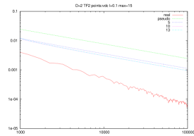
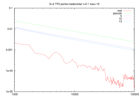
Figure 3: TF2, d=2 log-plot using a Van der Corput sequence (left) and a Niederreiter sequence (right). The classical error estimator is far off the real error whereas the quasi estimators are approaching the real error as more modes are added to the sum. The need for more modes is, however, obvious, in both plots.

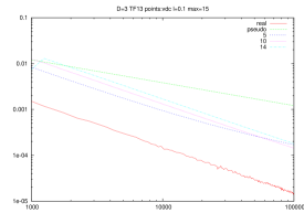
Figure 4: TF13, d=3 log-plot using a Van der Corput sequence (left) and a Niederreiter sequence (right). The quasi estimators follow the error with the appropriate $N$-dependence contrary to the pseudo estimator. Note that the $E^{q14}$ is in this case worse than $E^{q10}$ or $E^{q5}$ for all $N\leq 100000$. The higher modes converge slower to their average value, but the cross-over point is not known in advance and it is function-dependent.

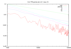
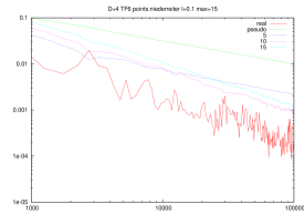
Figure 5: TF6, d=4 log-plot using a Van der Corput sequence (left) and a Niederreiter sequence (right). The quasi estimators approximate well the error. Moreover we see here a clearer instance of the crossover of higher modes in large $N$ mentioned in the previous figure.

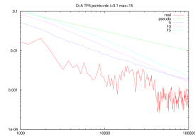
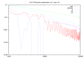
Figure 6: TF6, d=5 log-plot using a Van der Corput sequence (left) and a Niederreiter sequence (right). The use of the improved estimator (Eq.77) reduces the probability of a negative error square estimate but, naturally, it doesn’t remove it altogether. The plot on the right demonstrates this effect. As expected, the estimator returns to positive values and stabilizes as the number of points increases and the estimator converges to its average value.

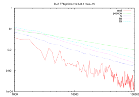
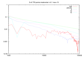
Figure 7: TF6, d=6 log-plot using a Van der Corput sequence (left) and a Niederreiter sequence (right). In this case the estimators describe very well the real error made in the integration.

4 Alternative approaches

4.1 Raising the value of $\lambda$ in the Jacobi diaphony

In general the real Quasi-Monte Carlo error is approached by including more and more modes in the estimator sum. At the same time, by including higher modes, one increases the error on this estimate (the error on $E_{2}$) because one attempts to estimate by Monte Carlo means the integral $\int f(\vec{x})e_{\vec{n}}(\vec{x})$ which will fluctuate vigorously for higher modes.

One might then attempt to raise the value of $\lambda$, thus decreasing the number of active modes (that give an appreciably non-zero $\omega_{\vec{n}})$). This would of course reduce the sensitivity of the diaphony, artificially lowering its value. Improvement in the error estimate originating from higher modes would be lost but the contribution of the modes close to the origin (which are the ones included) would be relatively enhanced, as can be seen from the behavior of the weights $\omega_{\vec{n}}$ (see Eq.66) .

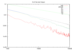
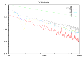
Figure 8: TF6, d=4 log-plot using the Van der Corput (left) and the Niederreiter (right) sequences. $E^{q15}$ is shown for different values of $\lambda$ indicated in the key, along with the real error and the classical estimate. Average values of all quantities for sets of 500 points are shown in each case. The value of $\lambda$ doesn’t alter the estimator, as long as that value stays within a specific range. We see that, in this case, the value $\lambda=1.6$ is out of the safe range.

4.2 Monitored estimator

The estimators $E^{q5}_{2}$ , $E^{q10}_{2}$ and $E^{q15}_{2}$ are not always proportional to the classical estimate, and, in some cases they decreases quite faster with $N$ than the classical estimate does. They never decrease slower than the classical estimate, though, and one can use that as follows. One monitors the ratio of $E^{q15}_{2}$, for example, to the ‘classical’ error estimate, and after a certain point, the ‘classical’ error is only estimated and multiplied with that ratio. This is a purely linear algorithm and therefore very fast. Caution has to be exercised, though, in the way the critical ration is chosen, in order to avoid configurations where the estimators acquire a very low value for some exceptional value of $N$.

This approach relies heavily on the, frequently false, assumption that the quasi and classical estimators scale. If this is not so, the new estimate is conservative. One has, thus, the option to trade accuracy for cpu time.

The plots of fig.9 show the ratio of $E^{q5}_{2}$ , $E^{q10}_{2}$ and $E_{2}^{q15}$ with $E_{2}$ for two particular cases.

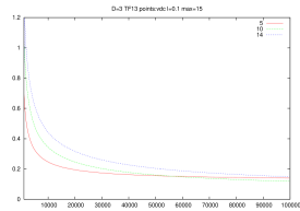
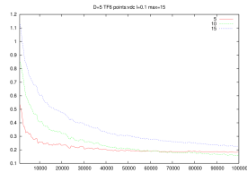
Figure 9: The ratio of different quasi estimators with the classical estimator for $d=3$ and TF13 (left) and $d=5$ TF6 (right). In both cases Van der Corput point-sets were used.

4.3 The box approximation

There is a choice for the diaphony that allows us to perform the integrals of Eq.(64) without resorting to the saddle point approximation. That choice is

$$\sigma_{\vec{n}}^{2}=\frac{1}{M}\prod_{\mu=1..d}\theta(n^{\mu}\leq m)$$ (84)

for some arbitrary $m$. The normalization (Eq.42) determines $M=(2m+1)^{D}-1$.

This diaphony includes only a finite number of modes, all of which are equally weighted. It can be seen as an approximation to the Jacobi diaphony since for small $\lambda$ the latter gives $\sigma_{\vec{n}}\approx 1$ for $|\vec{n}|\leq n_{c}$ and $\sigma_{\vec{n}}\approx 0$ for $|\vec{n}|\geq n_{c}$ where $n_{c}$ is determined implicitly by the value of the Jacobi diaphony. The diaphony can be evaluated as a quadratic function on the point-set from

$$S=\frac{1}{N}\sum_{\vec{n}}\sigma_{\vec{n}}^{2}|\sum_{i}e_{\vec{n}}(\vec{x})|^{2}=\frac{1}{NM}\sum_{|\vec{n}|\leq m}|\sum_{i}e_{\vec{n}}(\vec{x})|^{2}\equiv\frac{1}{NM}\sum_{i,j}\psi(\vec{x}_{i}-\vec{x}_{j})$$ (85)

with

$$\psi(\vec{x}_{i}-\vec{x}_{j})=-1+\prod_{\mu=1}^{D}\frac{sin\left((2m+1)\pi(x_{i}^{\mu}-x_{j}^{\mu})\right)}{sin\left(\pi(x_{i}^{\mu}-x_{j}^{\mu})\right)}$$ (86)

The distribution of point-sets with a particular value for $s$ is then found by explicitly performing the $z$-integrals of Eq.(64):

$$H(s)=\frac{K^{K}s^{K-1}}{\Gamma(K)}e^{-Ks}$$ (87)

with $K\equiv M/2$. Hence the correlation function is

$$F(s;\vec{x}_{i}-\vec{x}_{j})=\frac{(1-s)}{M}\psi(\vec{x}_{i}-\vec{x}_{j})$$ (88)

and the estimator of Eq.(72) becomes

$$E_{2}^{(q)}=\frac{1}{N^{2}}\sum f_{i}^{2}-\frac{1}{N^{3}}(\sum f_{i})^{2}-\frac{1}{N^{3}}\frac{(1-s)}{M}\sum_{i,j}\psi(\vec{x}_{i}-\vec{x}_{j})f_{i}f_{j}$$ (89)

This form has the advantage of including all modes up to an arbitrary $m$ without much effort, with the overhead, of course, of being quadratic in $N$. As $N$ grows beyond $10^{5}$ this becomes particularly impractical. For investigating purposes, however, this approach is useful in testing the behavior of $E_{2}^{(q)}$ with more modes included (that is presumably the small $\lambda$ limit).

It is remarkable that in the limit $m\rightarrow\infty$ we have $\psi(\vec{x}_{i}-\vec{x}_{j})=M\delta_{i,j}$, and this leads to $s=1$

$$E_{2}^{(q)}=\left(\frac{1}{N^{2}}\sum f_{i}^{2}-\frac{1}{N^{3}}(\sum f_{i})^{2}\right)$$ (90)

In that limit a good point-set would have to integrates well any mode using a finite number of points $N$. Since that is impossible, all point-sets will be evaluated as equally bad by the particular diaphony.

It is evident that one has to find an optimal value for $m$. In the following plot the estimator $E_{2}^{(q)}$ is shown for TF5 in 2 dimensions with different values for $m$ ranging from $3$ to $30$.

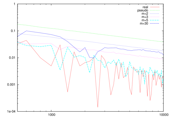
Figure 10: TF6, d=2 log-plot of the real error, and then from top to bottom the classical estimate, $E^{q}_{2}$ with $m=2$, with $m=3$ and $m=5$. The more modes one adds to the estimator the better it behaves. We also include the case $m=30$ (orange line), to demonstrate that there is a turning point in $m$ above which the estimate becomes worse. Note that $m=5$ means square length up to $2m^{2}=50$, much higher than $15$ that was our ceiling in the plots of the previous sections.

5 Concluding remarks

• The use of Quasi-Monte Carlo point-sets in numerical integration achieves a smaller error than the use of pseudo-random Monte Carlo point-sets. This advantage cannot be put in use without a reliable method for estimating the integration error.

• The ‘classical’, stochastic, error estimator relies on the assumption that the points in the point-set are uncorrelated. When used with a Quasi-Monte Carlo point-set, this assumption no longer holds. We saw that this leads to overestimating the error, thereby canceling any advantage gained by using the Quasi-Monte Carlo point-set.

• An estimator of stochastic nature is still possible but the underlying ensemble can not be the ensemble of all point-sets. We advocate the use of the ensemble of point-sets with the same degree of uniformity, as measured by a chosen diaphony. This approach leads to a prescription for a correlation function and an estimator, without the use of any information on the particular point-set or integrand.

• The price to pay is the raise in the computational complexity of the estimator from linear to quadratic in the number of points, which reflects the inclusion in the estimator of correlations between pairs of points. Using properties of diaphonies one can revert to a complexity that is linear times the number of modes involved.

• The error estimator suggested in this paper is shown to perform better than the ’classical‘ error estimator, resulting in an estimate up to an order of magnitude smaller than the ‘classical’ one.

• The flexibility of the construction (reflected in the freedom to choose the precise diaphony and the number of modes included) allows one to trade accuracy for computational cost. In computationally expensive applications, the monitoring approach of section 4.2 could be used to obtain an estimate that lies somewhere between the ‘classical’ and the quasi regime.

A number of further investigations have to be undertaken before implementing Quasi-Monte Carlo in the demanding field of phase space integration in particle physics. We defer these and further testing of the error estimator suggested above, in realistic cases, to further work.

acknowledgement

We would like to thank dr.C.Papadopoulos for persistently reminding us that a constant function can always be integrated with zero error.

Appendix A: Estimators by diagrammatics

Diagrammatics for Quasi-Monte Carlo and Monte Carlo

Our strategy for obtaining the form of the estimators is best described by an example. Consider the triple sum

$$S_{p_{1}}S_{p_{2}}S_{p_{3}}\equiv\sum\limits_{i,j,k=1}^{N}f_{i}^{p_{1}}f_{j}^{p_{j}}f_{k}^{p_{3}}\;\;.$$ (91)

In our approach we need to compute the expectation value of this object including the first sub-leading order in $1/N$. It is given by

$$\left\langle S_{p_{1}}S_{p_{2}}S_{p_{3}}\right\rangle = {N}^{\underline{3}}\int f_{i}^{p_{1}}f_{j}^{p_{j}}f_{k}^{p_{3}}\left(1-{1\over N}\left(F_{2}(i,j)+F_{2}(i,k)+F_{2}(j,k)\right)\right)$$ (92)

$$+{N}^{\underline{2}}\int\left(f_{i}^{p_{1}+p_{2}}f_{k}^{p_{3}}+f_{i}^{p_{1}+p_{3}}f_{j}^{p_{2}}+f_{i}^{p_{1}}f_{j}^{p_{2}+p_{3}}\right)+{\cal O}(N)$$

$$\approx N^{3}\int f_{i}^{p_{1}}f_{j}^{p_{j}}f_{k}^{p_{3}}-N^{2}\int f_{i}^{p_{1}}f_{j}^{p_{j}}f_{k}^{p_{3}}\left(\alpha_{ij}+\alpha_{ik}+\alpha_{jk}\right)$$

$$+N^{2}\int\left(f_{i}^{p_{1}+p_{2}}f_{k}^{p_{3}}+f_{i}^{p_{1}+p_{3}}f_{j}^{p_{2}}+f_{i}^{p_{1}}f_{j}^{p_{2}+p_{3}}\right)\;\;,$$

with implied integration over the subscripts. The sub-leading terms in the expectation value are, therefore, obtained by either connecting any two of the summands in the multiple sum $\Omega$ with a factor $-\alpha$, or by contracting them. Now, any estimator $E$ consists of a linear combination of terms like the above. Its variance, $\langle E^{2}\rangle-\left\langle E\right\rangle^{2}$, contains both leading and sub-leading terms. The leading terms, however, cancel completely, and so do the sub-leading terms coming from a connection/contraction inside one of the factors $E$. We arrive at the following diagrammatic prescription. A sum of powers of $f$ will be represented by a labeled dot, and a connection (including the $-\alpha$) by a link between dots. For example,

$$\raisebox{-14.22636pt}{\psfig{width=56.9055pt}}=\sum\limits_{i,j,k,l=1}^{N}f_{i}^{3}f_{j}f_{k}^{4}f_{l}^{2}\alpha_{jk}\alpha{kl}\;\;.$$ (93)

Now, suppose that the estimator $E$ is given as a linear combination of connected diagrams. The estimator of its variance is the given by the connected sub-leading diagrams that can be obtained from $E\times E$. The factors $1/N$ can be added in a straightforward manner: each sum with $p$ different summing indices carries a factor $N^{-p}$, and there is an additional overall factor $N^{1-2^{k}}$ in $E_{2^{k}}$.

Estimators for Quasi-Monte Carlo

We apply the above considerations to the first estimators $E^{(q)}_{1,2,4}$ for Quasi-Monte Carlo. Squaring and constructing the connected sub-leading diagrams, we find

$$E^{(q)}_{1} =$$

$$E^{(q)}_{2} = \raisebox{-8.5359pt}{\psfig{width=28.45274pt}}+\raisebox{-8.5359pt}{\psfig{width=8.5359pt}}$$

$$E^{(q)}_{4} = 4\;\raisebox{-8.5359pt}{\psfig{width=56.9055pt}}+4\;\raisebox{-8.5359pt}{\psfig{width=42.67912pt}}+4\;\raisebox{-8.5359pt}{\psfig{width=42.67912pt}}+4\;\raisebox{-8.5359pt}{\psfig{width=28.45274pt}}$$ (94)

$$+\;\raisebox{-8.5359pt}{\psfig{width=28.45274pt}}\;+\;\raisebox{-8.5359pt}{\psfig{width=11.38092pt}}\;\;.$$

Upon insertion of the correct factors of $1/N$, we arrive precisely at the estimators $E^{(q)}_{1,2,4}$ given in this paper. The construction of $E^{(q)}_{8}$ is straightforward: at that order, tree diagrams with branches develop. It may be worth noting that in this diagrammatic approach it becomes immediately clear that no diagrams with loops (that is, occurrences of $\alpha_{jj}$, or $\alpha_{ij}\alpha_{ji}$, or $\alpha_{ij}\alpha_{jk}\alpha_{ki}$, and so on) are possible to this order in $1/N$.

Estimators for Monte Carlo

The MC estimators are of course precisely those of Quasi-Monte Carlo, with the replacement $\alpha_{ij}\to 1$. This means that the topology of the tree diagrams becomes irrelevant, and we can feasibly go up to $E_{16}$. We find

$$E_{K}={1\over N^{2K-1}}\sum\limits_{s=0}^{K-1}E_{K,s}N^{s}\;\;\;,\;\;\;K=1,2,4,8,16\;\;,$$ (95)

where the coefficients of the various powers of $N$ are given by

$$E_{1,0} = S_{1}\;\;,$$ (96)

$$E_{2,0} = -S_{1}^{2}\;\;,$$

$$E_{2,1} = S_{2}\;\;,$$ (97)

$$E_{4,0} = -4S_{1}^{4}\;\;,$$

$$E_{4,1} = 8S_{1}^{2}S_{2}\;\;,$$

$$E_{4,2} = -S_{2}^{2}-4S_{1}S_{3}\;\;,$$

$$E_{4,3} = S_{4}\;\;,$$ (98)

$$E_{8,0} = -256S_{1}^{8}\;\;,$$

$$E_{8,1} = 1024S_{1}^{6}S_{2}\;\;,$$

$$E_{8,2} = -1152S_{1}^{4}S_{2}^{2}-512S_{1}^{5}S_{3}\;\;,$$

$$E_{8,3} = 352S_{1}^{2}S_{2}^{3}+832S_{1}^{3}S_{2}S_{3}+224S_{1}^{4}S_{4}\;\;,$$

$$E_{8,4} = -4S_{2}^{4}-224S_{1}S_{2}^{2}S_{3}-128S_{1}^{2}S_{3}^{2}-208S_{1}^{2}S_{2}S_{4}-96S_{1}^{3}S_{5}\;\;,$$

$$E_{8,5} = 32S_{2}S_{3}^{2}+8S_{2}^{2}S_{4}+48S_{1}S_{3}S_{4}+48S_{1}S_{2}S_{5}+32S_{1}^{2}S_{6}\;\;,$$

$$E_{8,6} = -S_{4}^{2}-8S_{3}S_{5}-4S_{2}S_{6}-8S_{1}S_{7}\;\;,$$

$$E_{8,7} = S_{8}\;\;,$$ (99)

$$E_{16,0} = -4194304S_{1}^{16}\;\;,$$

$$E_{16,1} = 33554432S_{1}^{14}S_{2}\;\;,$$

$$E_{16,2} = -104857600S_{1}^{12}S_{2}^{2}-16777216S_{1}^{13}S_{3}\;\;,$$

$$E_{16,3} = 162922496S_{1}^{10}S_{2}^{3}+93585408S_{1}^{11}S_{2}S_{3}+7733248S_{1}^{12}S_{4}\;\;,$$

$$E_{16,4} = -132579328S_{1}^{8}S_{2}^{4}-189530112S_{1}^{9}S_{2}^{2}S_{3}-20185088S_{1}^{10}S_{3}^{2}$$

$$-37552128S_{1}^{10}S_{2}S_{4}-3538944S_{1}^{11}S_{5}\;\;,$$

$$E_{16,5} = 54444032S_{1}^{6}S_{2}^{5}+172064768S_{1}^{7}S_{2}^{3}S_{3}+69861376S_{1}^{8}S_{2}S_{3}^{2}+63553536S_{1}^{8}S_{2}^{2}S_{4}$$

$$+15532032S_{1}^{9}S_{3}S_{4}+14942208S_{1}^{9}S_{2}S_{5}+1507328S_{1}^{10}S_{6}\;\;,$$

$$E_{16,6} = -9806848S_{1}^{4}S_{2}^{6}-69660672S_{1}^{5}S_{2}^{4}S_{3}-77729792S_{1}^{6}S_{2}^{2}S_{3}^{2}-45197312S_{1}^{6}S_{2}^{3}S_{4}$$

$$-43855872S_{1}^{7}S_{2}S_{3}S_{4}-5931008S_{1}^{8}S_{3}S_{5}-21135360S_{1}^{7}S_{2}^{2}S_{5}$$

$$-622592S_{1}^{9}S_{7}-5357568S_{1}^{8}S_{2}S_{6}-8060928S_{1}^{7}S_{3}^{3}-2802688S_{1}^{8}S_{4}^{2}\;\;,$$

$$E_{16,7} = 551936S_{1}^{2}S_{2}^{7}+14180352S_{1}^{5}S_{2}S_{3}^{3}+10500096S_{1}^{3}S_{2}^{5}S_{3}+32006144S_{1}^{4}S_{2}^{3}S_{3}^{2}$$

$$+12816384S_{1}^{4}S_{2}^{4}S_{4}+6193152S_{1}^{6}S_{2}S_{4}^{2}+36679680S_{1}^{5}S_{2}^{2}S_{3}S_{4}$$

$$+7016448S_{1}^{6}S_{3}^{2}S_{4}+13725696S_{1}^{6}S_{2}S_{3}S_{5}+11722752S_{1}^{5}S_{2}^{3}S_{5}$$

$$+2007040S_{1}^{7}S_{4}S_{5}+6072320S_{1}^{6}S_{2}^{2}S_{6}+1994752S_{1}^{7}S_{3}S_{6}$$

$$+250880S_{1}^{8}S_{8}+1798144S_{1}^{7}S_{2}S_{7}\;\;,$$

$$E_{16,8} = -256S_{2}^{8}-6438912S_{1}^{3}S_{2}^{2}S_{3}^{3}-3819520S_{1}^{2}S_{2}^{4}S_{3}^{2}-366592S_{1}S_{2}^{6}S_{3}$$

$$-1046016S_{1}^{2}S_{2}^{5}S_{4}-3568128S_{1}^{4}S_{2}^{2}S_{4}^{2}-8730624S_{1}^{4}S_{2}S_{3}^{2}S_{4}$$

$$-2233344S_{1}^{3}S_{2}^{4}S_{5}-1807360S_{1}^{5}S_{3}S_{4}^{2}-9879552S_{1}^{3}S_{2}^{3}S_{3}S_{4}$$

$$-8638464S_{1}^{4}S_{2}^{2}S_{3}S_{5}-2035712S_{1}^{5}S_{3}^{2}S_{5}-342016S_{1}^{6}S_{5}^{2}-2471936S_{1}^{4}S_{2}^{3}S_{6}$$

$$-3492864S_{1}^{5}S_{2}S_{4}S_{5}-1542144S_{1}^{5}S_{2}^{2}S_{7}-570368S_{1}^{6}S_{2}S_{8}-618496S_{1}^{6}S_{3}S_{7}$$

$$-607232S_{1}^{6}S_{4}S_{6}-851968S_{1}^{4}S_{3}^{4}-96256S_{1}^{7}S_{9}-3602432S_{1}^{5}S_{2}S_{3}S_{6}\;\;,$$

$$E_{16,9} = 542208S_{1}S_{2}^{4}S_{3}S_{4}+2359296S_{1}^{2}S_{2}^{2}S_{3}^{2}S_{4}+1404160S_{1}^{3}S_{2}S_{3}S_{4}^{2}$$

$$+1608704S_{1}^{3}S_{2}^{2}S_{3}S_{6}+514432S_{1}^{2}S_{2}^{3}S_{4}^{2}+924672S_{1}^{4}S_{3}S_{4}S_{5}$$

$$+765952S_{1}^{4}S_{2}S_{4}S_{6}+552960S_{1}^{2}S_{2}S_{3}^{4}+1405952S_{1}^{2}S_{2}^{3}S_{3}S_{5}$$

$$+1814528S_{1}^{3}S_{2}S_{3}^{2}S_{5}+540672S_{1}S_{2}^{3}S_{3}^{3}+1394688S_{1}^{3}S_{2}^{2}S_{4}S_{5}$$

$$+262656S_{1}^{2}S_{2}^{4}S_{6}+808960S_{1}^{4}S_{2}S_{3}S_{7}+90624S_{1}S_{2}^{5}S_{5}+575488S_{1}^{3}S_{3}^{3}S_{4}$$

$$+451584S_{1}^{4}S_{2}S_{5}^{2}+191488S_{1}^{5}S_{5}S_{6}+475136S_{1}^{4}S_{3}^{2}S_{6}+164864S_{1}^{5}S_{4}S_{7}$$

$$+422912S_{1}^{3}S_{2}^{3}S_{7}+179200S_{1}^{5}S_{3}S_{8}+343296S_{1}^{4}S_{2}^{2}S_{8}+167936S_{1}^{5}S_{2}S_{9}$$

$$+1024S_{2}^{6}S_{4}+33792S_{1}^{6}S_{10}+133760S_{1}^{4}S_{4}^{3}+60416S_{2}^{5}S_{3}^{2}\;\;,$$

$$E_{16,10} = -174336S_{1}S_{2}^{2}S_{3}S_{4}^{2}-191488S_{1}S_{2}S_{3}^{3}S_{4}-49920S_{1}^{2}S_{2}S_{4}^{3}-120832S_{1}S_{2}^{3}S_{3}S_{6}$$

$$-290304S_{1}^{2}S_{2}S_{3}^{2}S_{6}-183936S_{1}^{2}S_{2}^{2}S_{4}S_{6}-242688S_{1}S_{2}^{2}S_{3}^{2}S_{5}-99328S_{1}S_{2}^{3}S_{4}S_{5}$$

$$-87040S_{1}^{3}S_{4}^{2}S_{5}-231936S_{1}^{2}S_{2}^{2}S_{3}S_{7}-134400S_{1}^{3}S_{2}S_{4}S_{7}-153728S_{1}^{3}S_{2}S_{3}S_{8}$$

$$-174080S_{1}^{3}S_{2}S_{5}S_{6}-64512S_{2}^{3}S_{3}^{2}S_{4}-105216S_{1}^{2}S_{3}^{2}S_{4}^{2}-172288S_{1}^{3}S_{3}S_{4}S_{6}$$

$$-29184S_{2}^{4}S_{3}S_{5}-100352S_{1}^{2}S_{3}^{3}S_{5}-105472S_{1}^{3}S_{3}S_{5}^{2}-111360S_{1}^{2}S_{2}^{2}S_{5}^{2}$$

$$-90112S_{1}^{3}S_{3}^{2}S_{7}-22528S_{1}S_{2}^{4}S_{7}-40000S_{1}^{4}S_{4}S_{8}-47104S_{1}^{4}S_{5}S_{7}$$

$$-68608S_{1}^{3}S_{2}^{2}S_{9}-49088S_{1}^{2}S_{2}^{3}S_{8}-47616S_{1}^{4}S_{3}S_{9}-42240S_{1}^{4}S_{2}S_{10}$$

$$-10752S_{1}^{5}S_{11}-1152S_{2}^{4}S_{4}^{2}-23552S_{2}^{2}S_{3}^{4}-512S_{2}^{5}S_{6}-23296S_{1}^{4}S_{6}^{2}$$

$$-456960S_{1}^{2}S_{2}S_{3}S_{4}S_{5}-16384S_{1}S_{3}^{5}\;\;,$$

$$E_{16,11} = 3328S_{2}^{3}S_{5}^{2}+20352S_{2}^{2}S_{3}S_{4}S_{5}+16576S_{1}S_{2}S_{4}^{2}S_{5}+25088S_{1}S_{3}^{2}S_{4}S_{5}$$

$$+27136S_{1}S_{2}S_{3}S_{5}^{2}+4096S_{3}^{4}S_{4}+33024S_{1}^{2}S_{3}S_{5}S_{6}+26240S_{1}^{2}S_{2}S_{3}S_{9}$$

$$+32768S_{1}S_{2}S_{3}^{2}S_{7}+17536S_{1}S_{2}^{2}S_{4}S_{7}+5184S_{1}S_{3}S_{4}^{3}+24064S_{1}^{2}S_{3}S_{4}S_{7}$$

$$+25856S_{1}^{2}S_{2}S_{5}S_{7}+19456S_{1}S_{2}^{2}S_{3}S_{8}+16448S_{1}^{2}S_{2}S_{4}S_{8}+20224S_{1}S_{2}^{2}S_{5}S_{6}$$

$$+11392S_{2}S_{3}^{2}S_{4}^{2}+13440S_{1}^{2}S_{2}S_{6}^{2}+11328S_{1}^{2}S_{4}^{2}S_{6}+10240S_{2}S_{3}^{3}S_{5}$$

$$+16000S_{1}^{2}S_{4}S_{5}^{2}+224S_{2}^{4}S_{8}+11520S_{2}^{2}S_{3}^{2}S_{6}+832S_{2}^{3}S_{4}S_{6}+13312S_{1}S_{3}^{3}S_{6}$$

$$+13568S_{1}^{2}S_{3}^{2}S_{8}+9472S_{1}^{3}S_{6}S_{7}+6912S_{2}^{3}S_{3}S_{7}+9984S_{1}^{3}S_{5}S_{8}$$

$$+8832S_{1}^{3}S_{2}S_{11}+10368S_{1}^{3}S_{3}S_{10}+4224S_{1}S_{2}^{3}S_{9}+8576S_{1}^{3}S_{4}S_{9}$$

$$+10176S_{1}^{2}S_{2}^{2}S_{10}+352S_{2}^{2}S_{4}^{3}+46336S_{1}S_{2}S_{3}S_{4}S_{6}+3008S_{1}^{4}S_{12}\;\;,$$

$$E_{16,12} = -768S_{3}^{2}S_{5}^{2}-2944S_{2}S_{3}S_{5}S_{6}-1024S_{3}S_{4}^{2}S_{5}-2208S_{1}S_{2}S_{5}S_{8}-1664S_{1}S_{2}S_{4}S_{9}$$

$$-1216S_{2}S_{4}S_{5}^{2}-3072S_{1}S_{2}S_{3}S_{10}-2944S_{2}S_{3}S_{4}S_{7}-3584S_{1}S_{3}S_{5}S_{7}$$

$$-2944S_{1}S_{2}S_{6}S_{7}-2016S_{1}S_{3}S_{4}S_{8}-3008S_{1}S_{4}S_{5}S_{6}-768S_{1}^{2}S_{7}^{2}-1024S_{3}^{3}S_{7}$$

$$-1536S_{3}^{2}S_{4}S_{6}-1472S_{1}^{2}S_{6}S_{8}-224S_{2}S_{4}^{2}S_{6}-1920S_{1}S_{3}S_{6}^{2}-1024S_{1}S_{4}^{2}S_{7}$$

$$-1472S_{2}S_{3}^{2}S_{8}-1408S_{2}^{2}S_{5}S_{7}-208S_{2}^{2}S_{4}S_{8}-960S_{1}S_{2}^{2}S_{11}-1792S_{1}^{2}S_{3}S_{11}$$

$$-1440S_{1}^{2}S_{2}S_{12}-1312S_{1}^{2}S_{4}S_{10}-1792S_{1}S_{3}^{2}S_{9}-1088S_{2}^{2}S_{3}S_{9}$$

$$-1856S_{1}^{2}S_{5}S_{9}-768S_{1}S_{5}^{3}-128S_{2}^{2}S_{6}^{2}-704S_{1}^{3}S_{13}-4S_{4}^{4}-96S_{2}^{3}S_{10}\;\;,$$

$$E_{16,13} = 128S_{2}S_{7}^{2}+128S_{5}^{2}S_{6}+32S_{4}S_{6}^{2}+160S_{3}S_{5}S_{8}+48S_{2}S_{6}S_{8}+8S_{4}^{2}S_{8}$$

$$+256S_{3}S_{6}S_{7}+192S_{4}S_{5}S_{7}+128S_{3}^{2}S_{10}+224S_{1}S_{5}S_{10}+160S_{2}S_{5}S_{9}$$

$$+128S_{3}S_{4}S_{9}+192S_{1}S_{6}S_{9}+160S_{1}S_{7}S_{8}+224S_{1}S_{3}S_{12}+48S_{2}S_{4}S_{10}$$

$$+32S_{2}^{2}S_{12}+192S_{2}S_{3}S_{11}+128S_{1}S_{4}S_{11}+160S_{1}S_{2}S_{13}+128S_{1}^{2}S_{14}\;\;,$$

$$E_{16,14} = -S_{8}^{2}-16S_{5}S_{11}-16S_{7}S_{9}-8S_{6}S_{10}$$

$$-4S_{4}S_{12}-16S_{3}S_{13}-16S_{1}S_{15}-8S_{2}S_{14}\;\;,$$

$$E_{16,15} = S_{16}\;\;.$$ (100)

The number of individual terms in each $E_{K}$ is that of the partitions $\Pi(K)$ of $K$: $\Pi(1)=1$, $\Pi(2)=2$, $\Pi(4)=5$, $\Pi(8)=22$, and $\Pi(16)=231$. Likewise, the number of terms in each $E_{K,s}$ is the partition of $K$ into $(K-s)$ parts. We have not extended our results to the fifth-order error estimator with $K=32$ and $\Pi(32)=8349$, since already $E_{8}$ and $E_{16}$ are purely academic and we have included them only as an illustration of the method.

Appendix B: The $O(\frac{1}{N^{2}})$ contribution to $G_{p}$

The second order contribution to $G_{p}$ can be found by summing up $O(\frac{1}{N^{2}})$ terms coming from

1. the pure rings (containing only 2-point vertices)

2. the three graphs contributing to $G_{p}^{(1,2,3)}$ (containing one 4-vertex, two 3-vertices or two external points)

3. products of a pure ring and one of the three graphs above or two of the graphs above.

4. the new graphs (containing one 6-vertex,one 5-vertex and one 3-vertex, two 4-vertices, one 4-vertex and two 3-vertices, four 3-vertices, one 3-vertex and three external points, two 3-vertices and two external points or one 4-vertex and two external points)

After a lengthy but straightforward calculation (involving some cancellations) we get

$$G_{p}^{(3)} =\frac{G_{0}p}{N^{2}} (\;\frac{2p-1}{4}K_{3}-\frac{1}{4}(K_{2})^{2}-\frac{1}{2}K_{2}(x_{i},x_{j})\;)$$

$$+\frac{G_{0}}{N^{2}} (\;\;\frac{3}{8}K_{5}+\frac{1}{3}K_{4}-\frac{1}{32}K_{3}^{2}-\frac{1}{8}K_{2}K_{1}(x_{i},x_{j})$$

$$-\frac{1}{2}K_{3}(x_{i},x_{j})-\frac{1}{12}L_{1,1,1}-\frac{1}{2}L_{2,1,1}-\frac{1}{4}L_{2,2,1}$$

$$-\frac{1}{48}K_{3}L_{1,1,1}-\frac{1}{4}L_{3,1,1}+\frac{1}{8}K_{1}(x_{i},x_{j})^{2}+\frac{1}{2}Q_{1}(x_{i},x_{j},x_{k})$$

$$+\frac{1}{4}Q_{2}(x_{i},x_{j})+\frac{1}{2}Q_{3}(x_{i},x_{j},x_{k})+\frac{1}{4}Q_{4}(x_{i},x_{j})$$

$$+\frac{1}{6}L_{1,1,1}(x_{i},x_{j},x_{k})+\frac{1}{24}L_{1,1,1}K_{1}(x_{i},x_{j})+\frac{1}{288}L_{1,1,1}^{2}$$

$$+\frac{1}{48}M_{1}+\frac{1}{8}M_{2}+\frac{1}{24}M_{3}+\frac{1}{16}M_{4})$$

where

$$K_{a,b,\ldots}\equiv\sum_{1,2,\ldots}\rho_{1}^{a}\rho_{2}^{b}\ldots$$ (101)

$$K_{a}(x_{i},x_{j})\equiv\sum^{\prime}_{i,j}\sum_{1}\rho_{1}^{a}e_{\vec{n}_{1}}(x_{i})e^{*}_{\vec{n}}(x_{j})$$ (102)

$$L_{a,b,c}\equiv\sum_{1,2,3}\rho_{1}^{a}\rho_{2}^{b}\rho_{3}^{c}\delta_{1+2+3}$$ (103)

$$Q_{1}(x_{i},x_{j},x_{k})\equiv\sum^{\prime}_{i,j,k}\sum_{1,2}\rho_{1}\rho_{2}e_{\vec{n}_{1}}(x_{i})e^{*}_{\vec{n}_{1}}(x_{j})e_{\vec{n}_{2}}(x_{j})e^{*}_{\vec{n}_{2}}(x_{k})$$ (104)

$$Q_{2}(x_{i},x_{j})\equiv\sum^{\prime}_{i,j}\sum_{1,2}\rho_{1}\rho_{2}e_{\vec{n}_{1}}(x_{i})e_{\vec{n}_{1}}^{*}(x_{j})e_{\vec{n}_{2}}^{*}(x_{i})e_{\vec{n}_{2}}(x_{i})$$ (105)

$$Q_{3}(x_{i},x_{j},x_{k})\equiv\sum^{i}_{i,j,k}\sum_{1,2,3}\rho_{1}\rho_{2}e_{\vec{n}_{1}}(x_{i})e_{\vec{n}_{1}}^{*}(x_{j})e_{\vec{n}_{2}}(x_{j})e_{\vec{n}_{2}}^{*}(x_{k})e_{\vec{n}_{3}}(x_{j})e_{\vec{n}_{3}}^{*}(x_{k})$$ (106)

$$Q_{4}(x_{i},x_{j})\equiv\sum_{i,j}\sum_{1,2}\rho_{1}^{2}\rho_{1+2}e_{\vec{n}_{1}}(x_{i})e_{\vec{n}_{1}}^{*}(x_{j})$$ (107)

$$L_{a,b,c}(x_{i},x_{j},x_{k})\equiv\sum^{\prime}_{i,j,k}\sum_{1,2,3}\rho_{1}^{a}\rho_{2}^{b}\rho_{3}^{c}e_{\vec{n}_{1}}(\vec{x}_{i})e_{\vec{n}_{2}}(\vec{x}_{j})e_{\vec{n}_{3}}(\vec{x}_{k})\delta_{1+2+3}$$ (108)

$$Q_{a,b}(x_{i},x_{j},x_{k})\equiv\sum^{\prime}_{i,j,k}\sum_{1,2}\rho_{1}^{a}\rho_{2}^{b}e_{\vec{n}_{1}}(\vec{x}_{i})e^{*}_{\vec{n}_{1}}(\vec{x}_{j})e_{\vec{n}_{2}}(\vec{x}_{j})e^{*}_{\vec{n}_{2}}(\vec{x}_{k})$$ (109)

$$M_{1}\equiv\sum_{1,2,3,4}\rho_{1}\rho_{2}\rho_{3}\rho_{4}\delta_{1+2+3+4}$$ (110)

$$M_{2}\equiv\sum_{1,2,3,4,5}\rho_{1}\rho_{2}\rho_{3}\rho_{4}\rho_{5}\delta_{1+2-5}\delta_{3+4-1-2}\delta_{5-3-4}$$ (111)

$$M_{3}\equiv\sum_{1,2,3,4,5,6}\rho_{1}\rho_{2}\rho_{3}\rho_{4}\rho_{5}\rho_{6}\delta_{1-2-5}\delta_{2-3-6}\delta_{3-1-4}\delta_{4+5+6}$$ (112)

$$M_{4}\equiv\sum_{1,2,3,4,5,6}\rho_{1}\rho_{2}\rho_{3}\rho_{4}\rho_{5}\rho_{6}\delta_{1-2-5}\delta_{2-3-6}\delta_{3+6-4}\delta_{4-5-1}$$ (113)

with

$$\rho_{i}\equiv\frac{2z\sigma^{2}_{\vec{n}_{i}}}{1-2z\sigma^{2}_{\vec{n}_{i}}}$$ (114)

and $\sum^{i}_{i,j,k,\ldots}=\sum_{\vec{x}_{i}\neq\vec{x}_{j}\neq\vec{x}_{k}\ldots}$, $\sum_{1,2,\ldots}\equiv\sum_{\vec{n}_{1},\vec{n}_{2},\ldots}$ and $\delta_{1+8-2+\ldots}\equiv\delta(\vec{n}_{1}+\vec{n}_{8}-\vec{n}_{2}+\ldots)$.

References

- [1] Douglas Adams, ”The Hitchhiker’s Guide to the Galaxy”, Pan London, 1979.
- [2] Hoogland and Kleiss Comp.Phys.Comm.98:128-136,1996 [hep-ph/9601270]
- [3] Hoogland and Kleiss Comp.Phys.Comm.101:21-30,1997 [hep-ph/9609244]
-
[4]
M.Luescher, Comp.Phys.Comm.,79,100 (1994)
F.James,Comp.Phys.Comm.,79,110 (1994) - [5] Halton, Num.Math. 2, 84-90 (1960)
- [6] Ch.Schlier Comp.Phys.Comm., 159,93 (2004)
- [7] H.Niederreiter J.Number Theory 30 (1988) 51-70
- [8] P.Bratley, B.Fox and H.Niederreiter AMC Transactions on Modeling and Computer Simulation 2,No.3 (1992),195-213
- [9] A.Owen, Monte Carlo extension of Quasi Monte Carlo, Winter Simulation Conference, IEEE Press, 1998