Non-extensive Boltzmann Equation and Hadronization

Abstract

For a general, associative addition rule defining a non-extensive thermodynamics we construct the strict monotonic function, which transforms it to a normal extensive quantity. We investigate the evolution of the one-particle distribution in the framework of a two-body Boltzmann equation supported with a non-extensive energy addition rule. An H-theorem can be proven for the extensive function of the non-extensive entropy. The equilibrium distribution is exponential in the extensive quantity associated to the original one-particle energy with the non-extensive addition rule. We propose that for describing the hadronization of quark matter non-extensive rules may apply.

There are several experimental evidences on power-law tailed statistical distributions of single particle energy, momenta or velocity. In particular hadron transverse momentum spectra at central rapidity, which stem from elementary particle and heavy ion collisions, can be well fitted by a formula reflecting $m_{T}$-scalingPHENIX ; STAR ; ZEUS ; MAREK ; BECK ; TASSO ; MT-SCALING ; T-TEAM-FITS :

$$f(p_{T})\sim\left(1+m_{T}/E_{c}\right)^{-v}.$$ (1)

Interpreting these spectra as a distribution in the transverse directions at zero rapidity, the single particle energy is given by $E=m_{T}=\sqrt{p_{T}^{2}+m^{2}}$ for a relativistic particle with mass $m$ (in units setting the lightspeed to $c=1$). Amazingly this formula describes exactly the Tsallis distribution $f(E)$, which was obtained by using theoretical arguments of thermodynamical natureTSALLIS-ENTROPY . Distributions with power-law like tail, in particular the Tsallis distribution, can be seen in many areas where statistical models applyMULT-NOISE ; WILK ; BIALAS ; FLORKOW ; KODAMA ; RAF-BOLTZMANN-EQ ; WAL-RAFELSKI ; TSB-RHIC-SCHOOL ; ASTRO . It was investigated as a generic feature in the framework of non-extensive thermodynamicsTSALLIS-RULES ; TSALLIS-WANG ; TSALLIS-FOKKER . Tsallis has suggested an expression for the entropy, also encountered earlier by othersTSALLIS-ENTROPY ; OTHER-ENTROPIES , which would be an alternative to the Boltzmann formula. From this, with a canonical constraint on the total energy, the distribution (1) can be derived. Without being able to exclude a non-equilibrium interpretation of the power-law tail, it is tempting to investigate the possibility that some non-exponential spectra would be a result of a particular form of equilibrium, featuring characteristics of a non-extensive thermodynamics.

In this paper we propose a possible way to understand power-law tailed energy distributions as equilibrium solutions to a slightly generalized two-body Boltzmann equation. More specifically we show that this two-body Boltzmann-equation allows for non-exponential stationary single-particle distributions, if the two-body distribution factorizes, but the two-body energy is not extensive. The Tsallis distribution is a special case thereof. The pair-energy, typical for generating this distribution, is a product of the single particle energies.

It is a widespread belief that only the exponential distribution can be the stationary solution to the Boltzmann equation, but this statement is true only with a few restrictions: i) if the two-particle distributions factorize, ii) the two-particle energies are additive in the single-particle energies ($E_{12}=E_{1}+E_{2}$ ) and iii) the collision rate is multilinear in the one-particle densities.

A generalization of the original Boltzmann equation has been pioneered by KaniadakisBOLTZMANN-GENERAL considering a general, nonlinear density dependence of the collision rates. An ${}^{\prime\prime}H_{q}^{\prime\prime}$ theorem for the particular Tsallis form of the collision rate has been derived by Lima, Silva and PlastinoHQ-THEOREM . Here we follow another ansatz, we modify the linear Boltzmann equation in the energy balance part only: Instead of requiring $E_{1}+E_{2}=E_{3}+E_{4}$ in a $1+2\leftrightarrow 3+4$ two-body collision we consider a general, not necessarily extensive, rule:

$$h(E_{1},E_{2})\>=\>h(E_{3},E_{4}).$$ (2)

It is physically sensible to choose the function $h(x,y)$ symmetric and satisfying $h(E,0)=h(0,E)=E$. Also, for applying the same rule for subsystems combined themselves of subsystems, associativity is required: $h(h(x,y),z)=h(x,h(y,z))$. This way the same rule applies for the elementary two-particle system as for large subsystems in the thermodynamical limit. It is known that the general mathematical solution of the associativity requirement is given by

$$h(x,y)\>=\>X^{-1}\left(X(x)+X(y)\right),$$ (3)

with $X(0)=0$ and $X(t)$ being a continuous, strict monotonic functionFUNC-EQ-MATH . Composing the formula (3) with the function $X$ and taking the partial derivative with respect to $y$ at $y=0$ one obtains an ordinary differential equation for $X(x)$ with the solution

$$X(E)\>=\>X^{\prime}(0)\,\int_{0}^{E}\frac{dx}{\frac{\partial h}{\partial y}(x,0)}.$$ (4)

Due to $X(h(E_{1},E_{2}))=X(E_{1})+X(E_{2})$, the quasi-energy $X(E)$ is an additive quantity and the rule (2) is equivalent to

$$X(E_{1})\,+\,X(E_{2})\>=\>X(E_{3})\,+\,X(E_{4}).$$ (5)

Applying such a general energy addition rule (5), the rate of change of the one-particle distribution is given by

$$\frac{\partial f(p_{1})}{\partial t}=\int_{p_{2},p_{3},p_{4}}\!\!\!\!\!\!\!\!\!\!\!\!\!\!\!{\cal W}(p_{1},p_{2};p_{3},p_{4})\Delta\,\left[f(p_{3})f(p_{4})-f(p_{1})f(p_{2})\right].$$ (6)

with the symmetric transition probability ${\cal W}$ and the constraint

$$\Delta\>=\>\delta^{3}(\vec{p}_{1}+\vec{p}_{2}-\vec{p}_{3}-\vec{p}_{4})\,\delta\left(h(E_{1},E_{2})-h(E_{3},E_{4})\right).$$ (7)

In equilibrium the distributions depend on the phase space points through the energy variables only and the detailed balance principle requires

$$f(E_{1})\,f(E_{2})\>=\>f(E_{3})\,f(E_{4}).$$ (8)

With the generalized constraint (7) this relation is satisfied by

$$f(E)\>=\>f(0)\exp(-X(E)/T)$$ (9)

with $1/T=-f^{\prime}(0)/f(0)$ and $X(E)$ given by eq.(4). In the extensive case $h(x,y)=x+y$ leads to $X(E)=E$, for the Tsalis-type energy addition ruleTSALLIS-RULES ; TSALLIS-WANG ,

$$h(x,y)=x+y+axy,$$ (10)

one obtains $X(E)\>=\>\frac{1}{a}\ln(1+aE)$ and

$$f(E)\>=\>f(0)\left(1+aE\right)^{-1/aT}.$$ (11)

Since the energy addition rule (2) conserves the quantity $h(E_{1},E_{2})$ in a microcollision, the new energies after the collision also lie on the $h$=constant line. Due to the additivity of the quasi-energy, $X(E)$, the total sum $X_{tot}=\sum_{i}X(E_{i})$, is a conserved quantity. This rule can be applied in numerical simulations, too. Since our present goal is to find the equilibrium only, we may assume constant transition probabilities.

Fig.1 presents results of a simple test particle simulation with the rule (10). We mostly started with a uniform energy distribution between zero and $E_{0}=1$ with a fixed number of particles $N=10^{4}$ (red, full line). The one-particle energy distribution evolves towards the well-known exponential curve for $a=0$, shown in the left part of Fig.1. This snapshot was taken after $200$ two-body collisions per particle (blue, short dashed line). The analytical fit to this histogram is given by $2e^{-E/T}$ (with $T=E_{0}/2=0.5$ in this case). An intermediate stage of the evolution after $0.4$ collisions per particle is also plotted in this figure (green, long dashed line). Using the prescription (10) with $a=1$, the stationary solution becomes a Tsallis distribution. The numerical evolution from the uniform energy distribution can be inspected in the right side of Fig.1. The fit to the final curve is given by $f(E)=2.6(1+aE)^{-3.6}$. All distributions are normalized to one.

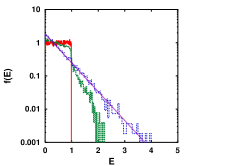
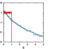
Figure 1: (Color online) Evolution towards the Boltzmann distribution for $a=0$ (left part) and towards the Tsallis one for $a=1$ (right part) using $h(E_{1},E_{2})=E_{1}+E_{2}+aE_{1}E_{2}$. For detailed explanation see text.

It is in order to make some remark on the energy conservation. For $h(x,y)=x+y$ we simulate a closed system with elastic collisions: The sum, $U=\sum_{i=1}^{N}E_{i}$, does not change in any of the binary collisions. The situation changes by using a non-extensive formula for $h(x,y)$, like in the case of the Tsallis prescription. With a constant positive (negative) $a$, the bare energy sum, $U$, is decreasing (increasing) while approaching the stationary distribution. This is typical for open systems gaining or loosing energy during their evolution towards a stationary state.

One may incline to consider the conserved quasi-energy, $X(E)$, as an in-medium one particle energy. The interesting point is that in general any prescription, $h(E_{1},E_{2})$ – defining a version of the non-extensive thermodynamics –, is equivalent to considering a quasi-energy, $X(E)$. For small energies one expects a restoration of the extensive rule and $X(E)\approx E$, $X^{\prime}(0)=1$. Whenever the pair energy is repulsive (attractive), $h(E_{1},E_{2})\geq E_{1}+E_{2}$ ($h(E_{1},E_{2})\leq E_{1}+E_{2}$), a rising quasi-energy is smaller (bigger) than the free one, $X(E)\leq E$ ($X(E)\geq E$). This leads to a tail of the stationary distribution in the free single particle energy, $f(E)$, which is above (below) the exponential curve. This phenomenon is hard to distinguish from a power-law tail numerically.

The question arises that – constrained by the conserved number of particles, $N=\int f\,d\Gamma$, and the total quasi-energy, $X_{{\rm tot}}\,=\,\int f\,X(E)\,d\Gamma$, – what is the proper formula for the entropy which grows when approaching the stationary distribution. If the addition rule of the non-extensive entropy, $s$, is given by $h_{s}(x,y)$, then the quasi-entropy, $X_{s}(s)$, is additive and the total entropy is given by

$$X_{s}(S_{tot})\>=\>\int\!f\,X_{s}(s(f))\,d\Gamma=\int\!\sigma(f)\,d\Gamma.$$ (12)

Its rate of change, $\dot{X}_{s}(S_{tot})\>=\>\int\dot{f}\,\sigma^{\prime}(f)\,d\Gamma$ can be expressed with the help of the Boltzmann equation (6).

Assuming the symmetry properties $1\leftrightarrow 2$, $3\leftrightarrow 4$ and $(12)\leftrightarrow(34)$ for the constrained rate factor $w_{1234}={\cal W}\Delta$, one easily derives

$$X_{s}^{\prime}(S_{tot})\>\dot{S}_{tot}\>=\>\frac{1}{4}\int_{1234}\!\!w_{1234}\left(f_{3}f_{4}-f_{1}f_{2}\right)\,\times$$

$$\left(\sigma^{\prime}(f_{1})+\sigma^{\prime}(f_{2})-\sigma^{\prime}(f_{3})-\sigma^{\prime}(f_{4})\right).$$ (13)

A definite sign for this quantity can be obtained due to the additivity of $X_{s}(s(f))=\sigma(f)/f$, leading to the unique solution $X_{s}(s(f))=B\ln f$ . For $B=-k_{B}$ (Boltzmann’s constant) $\dot{S}_{tot}\geq 0$ follows. Using the $k_{B}=1$ unit system we arrive at $X_{s}(s(f))=-\ln f$, and the expression for the total additive quasi-entropy (12), coincides with Boltzmann’s original suggestion. At the same time, applying a non-extensive addition rule for the entropy, $h_{s}(x,y)=x+y+(1-q)xy$, as Tsallis did, we have $X_{s}(s)=\frac{1}{1-q}\ln(1+(1-q)s)$ (Abe’s formulaABE ), and from $X_{s}(s)=-\ln f$ one obtains Tsallis’ entropy formula

$$fs(f)=\frac{f^{q}-f}{1-q}.$$ (14)

In numerical simulations we observe that the Tsallis-type non-extensive energy addition rule, applied to a test-particle simulation with two-body collisions, maximizes the Boltzmann-quasi-entropy (cf. Fig.2). The stationary distribution is nevertheless a Tsallis distribution (cf. Fig.1).

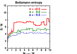
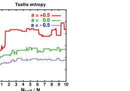
Figure 2: (Color online) Evolution of the Boltzmann and Tsallis entropies by applying the energy addition rule $h(E_{1},E_{2})=E_{1}+E_{2}+aE_{1}E_{2}$ with different values of the parameter $a$.

It is interesting to note that, as in many papersTSALLIS-RULES , applying a canonical constraint on the bare total energy, $U=\int\!Ef(E)\,d\Gamma$, when seeking for the equilibrium distribution one obtains equivalent results for the Tsallis case. Instead of using the (due to the H-theorem guaranteed correct) formula,

$$\frac{d}{df}\left(fX_{s}(s(f))\right)\>=\>\alpha+\beta X(E),$$ (15)

where $X_{s}(s)$ and $X(E)$ are both Tsallis-like expressions, the naive assumption of

$$\frac{d}{df}\left(fs(f)\right)\>=\>\alpha+\beta E,$$ (16)

also leads also to a power-law distribution. In the first case $X_{s}(s(f))=-\ln f$ independently of the non-extensive rule definition for the entropy, and the equilibrium solution is $f_{eq}\propto\exp(-X(E)/T)=(1+aE)^{-1/(aT)}$ with $\beta=1/T$. In the second case the particular form of $s(f)$ is used and the non-extensive addition rule for the energy is ignored. (This case has nothing to do with our simulation.) The distribution resulting from (16) is $f_{eq}\propto(1+aE/(1+\alpha aE))^{-1/(aT)}$ when $q=1-aT$.

In numerical simulations both the Boltzmann and the Tsallis entropy increase, disregarding the fluctuations due to the finite number of test particles, $N=10^{4}$, and due to finite binning resolution in energy, ($N_{bin}=100$ while the maximal energy, $E_{max}$ is changing). The increase is a trend, it is not rigorously fulfilled in each microscopic collision; it is a common behavior of molecular dynamical simulations. The ratio of the two entropy expressions also fluctuates somewhat, but the Tsallis entropy in the repulsive (attractive) case clearly stays bigger (smaller) than the Boltzmann entropy.

Physical realizations of non-extensive systems may be discovered depending on our knowledge about the microscopical forces influencing the particles during the pair-interactions. For such forces being repulsive, the canonical one-particle energy distribution has a tail above the exponential curve, for attractive interactions below. As a rule, as long as this modification is small, it is extremely difficult to see the non-exponential tail in the bare one-particle energy distribution both in experiments and in numerical simulations. Such power-law tails are prominent in elementary particle spectra in high energy experiments, but their traditional explanation does not assume an equilibrium state.

In the quark-gluon plasma (QGP), or more generally in a parton matter before hadronization color non-singlet objects are the single particles. Eventually all form hadrons, in the soft sector perhaps by recombination and in the hard sector dominantly by fragmentation. In both cases a long-range interaction between color non-singlet partons, connected to the physical phenomenon confinement, is present in the background. In the following we consider a simple model for including this type of non-perturbative pair-interaction.

For the sake of simplicity let us restrict ourselves to two body processes between color triplets and anti-triplets. This is the most common way of meson formation. It is also an important part of baryon formation due to quark - diquark fusion. The pairs of such partons, while they constantly interact, are either in a color singlet or in a color octet state (in a QGP in one case from nine a singlet, otherwise an octet). The energy of the two-parton system is given by

$$E^{{\rm\>color\,state}}_{12}=E_{1}+E_{2}+\Delta^{{\rm color\,state}},$$ (17)

where the singlet channel should be attractive (relative to the free partons). The color average is supposed to be vanishing, $\Delta^{{\rm singlet}}+8\Delta^{{\rm octet}}=0$. This is certainly the case for interactions like in the Heisenberg-model of magnets, where the pair-potential is proportional to the product of symmetry generators in the corresponding spin representation. For SU(3) color this is also the case. The singlet charge is zero, the octet charge square is $Q^{2}_{{\rm octet}}=3$. The triplet and anti-triplet both have $Q^{2}_{{\rm triplet}}=4/3$. The Heisenberg-magnet-like interaction in color has therefore a factor of $-8/3$ for the singlet and a factor of $3-8/3=1/3$ for the octet. Their degeneracy-weighted sum is zero.

For considering the possibility of a non-Boltzmann distribution in quark matter we further assume a Coulomb-like interaction. In this case $\Delta^{{\rm singlet}}\>=\>2E_{12}^{{\rm\>rel.kin.}}$ from the binding in the color singlet channel. For the search after a stationary single-quark distribution of the two-body Boltzmann equation in the octet channel it accounts to consider,

$$E_{12}^{{\rm\>octet}}\,=\,E_{1}\>+\>E_{2}\>+\>\frac{1}{4}\>E_{12}^{{\rm\>rel.kin.}}.$$ (18)

The rest is kinematical consideration. We assume the coalescence of two massless partons to a (nearly) massless hadron. Due to the triangle inequality, the kinetic energy of the relative motion of two massless partons is non-negative,

$$E_{12}^{{\rm\>rel.kin.}}=|\vec{p}_{1}+\vec{p_{2}}|-|\vec{p}_{1}|-|\vec{p}_{2}|\geq 0.$$ (19)

For small relative angles between the momentum vectors, $\vartheta$, this is approximated by

$$E_{12}^{{\rm\>rel.kin.}}=\frac{2E_{1}E_{2}\,\sin^{2}(\vartheta/2)}{E_{1}+E_{2}}$$ (20)

The sum of the individual parton energies in the same approximation is close to $E_{1}+E_{2}\approx P=|\vec{p}_{1}+\vec{p}_{2}|$. Even very hard partons with a high value of the total pair momentum, $P$, need a little relative motion for interacting: in the singlet channel to eventually form hadrons, in the octet channel to maintain a single-particle quark-distribution typical for the pre-hadronic phase. The stationary version of this distribution, while detailed balance is satisfied on the two-body level, is often found to be close to the Tsallis distribution. We propose that the above mechanism, from the comparison of eqs.(10), (18) and (20) leading to

$$E_{c}=1/a=\frac{2P}{\sin^{2}(\vartheta/2)},$$ (21)

may be in the background of such findings. Asymptotical freedom is recovered as for very fast partons $E_{c}\rightarrow\infty$ with $P\rightarrow\infty$, and so the one particle energies of a colliding pair become additive.

In conclusion we have investigated deterministic, non-extensive energy addition rules in two-body collisions. We have pointed out that instead of the one-particle energy a quasi-energy is conserved by such rules in each collision, leading to a non-Boltzmannian stationary distribution in the bare one-particle energy. In particular the Tsallis distribution is obtained by using a Tsallis-type non-extensive energy addition rule. The corresponding conserved quasi-energy is identical to that proposed by Q.WangTSALLIS-WANG . Modifications to the extensive energy addition rule may have to be considered if there is a statistically important pair-interaction between particles. The stationary canonical distribution becomes exponential in the conserved quasi-energy $X(E)$, but it is non-exponential in terms of the free particle energy $E$. The Boltzmann entropy, $S_{B}=X_{s}(S_{tot})=-\int f\ln fd\Gamma$, is never decreasing and reaches its maximum at this distribution. Alternative expressions for the entropy, in particular the one promoted by Tsallis, correspond to a non-extensive entropy addition rule which defines $X_{s}(s)$. Notably, in the Tsallis case also the naive integral, $S_{T}=\int fs(f)d\Gamma$, seem to increase in numerical simulations as the elementary collisions proceed. The Tsallis-type energy and entropy addition rules are correlated by $q=1-aT$.

As a possible physical realization we have proposed a mechanism leading to nearly Tsallis-distributed quarks in quark matter and hadrons which eventually form. This mechanism considers a color state dependent pair-energy based on general arguments describing a quantum symmetry. The essential clue leading to our result then hides in the use of a virial theorem which connects the color interaction with kinematical factors of the quark pair. In a certain approximation the modification of the familiar two-body energy conservation factor in the Boltzmann equation receives a term proportional to the product of single-quark kinetic energies to leading order in the ultrarelativistic expansion. The Tsallis distribution turns out to be an approximation next simplest to the original Boltzmannian one.

Our picture naturally connects the processes maintaining a possible stationary distribution among colored partons with the hadronization process. In the approximation discussed in this paper the power of the power-law tail in hadronic spectra equals to the power occurring in the single-quark distribution in quark matter. As a consequence mesonic and baryonic powers are also equal to each other. This agrees with experimental findings well, although the recombination assumption predicting a baryonic to mesonic power ratio of $3:2$ also cannot be excluded, when considering the relatively high error bars. This result is, however, simpler and more generic. Here only a balance between kinetic and potential energy in the relative motion of quarks has been assumed besides some basic color properties of the pairwise interaction.

Acknowledgment

Enlightening discussions with Prof. Carsten Greiner and Dr. Zhe Xu at the University of Frankfurt as well as with Drs. Géza Györgyi at Eötvös University and Antal Jakovác at the Technical University Budapest are hereby gratefully acknowledged. This work has been supported by the Hungarian National Science Fund OTKA (T034269, T49466) and the Deutsche Forschungsgemeinschaft due to a Mercator Professorship for T.S.B.

References

- (1) PHENIX collaboration: J. M. Heuser et.al. Acta Phys. Hung. Heavy Ion Phys. 15, 291, 2003; K. Adcox et.al. Phys.Rev.C 69, 024904, 2004; S. S. Adler et.al. Phys.Rev.C 69, 034909, 034910, 2004; K. Reygers et.al. Nucl.Phys.A 734, 74, 2004.
- (2) STAR collaboration: C. Adler et.al. Phys.Rev.Lett. 87, 112303, 2001; J. Adams et.al. Phys.Rev.Lett. 91, 172302, 2003; A. A. P. Suaide et.al. Braz.J.Phys. 34, 300, 2004; R. Witt, nucl-ex/0403021.
- (3) ZEUS collaboration: Eur.Phys.J. C11, 251, 1999.
- (4) I. Bediaga, E. M. F. Curado, J. M. de Miranda, Z.Phys.C 22, 307, 1984; Z.Phys.C 73, 229, 1997.
- (5) M. Gazdzicki, M. Gorenstein, Phys.Lett.B 517, 250, 2001.
- (6) C. Beck, Physica A 286, 164, 2000, cond-mat/0301354, hep-ph/0004225.
- (7) J. Schaffner-Bielich, D. Kharzeev, L. McLerran, R. Venugopalan, Nucl.Phys.A 705, 494, 2002.
- (8) T. S. Biro, G. Györgyi, A. Jakovác, G. Purcsel, hep-ph/0409157.
- (9) C. Tsallis, J.Stat.Phys. 52, 50, 1988; Physica A 221, 277, 1995; Braz.J.Phys. 29, 1, 1999; P. Prato, C. Tsallis, Phys.Rev.E 60, 2398, 1999; V. Latora, A. Rapisarda, C. Tsallis, Phys.Rev.E 64, 056134, 2001; Physica A 305, 129, 2002.
- (10) C. Anteneodo, C. Tsallis, Physica A 324, 89, 2003; T. S. Biró, A. Jakovác, hep-ph/0405202.
- (11) G. Wilk, Z. Wlodarczyk, Physica A 305, 227, 2002; Chaos, Solitons and Fractals 13, 581, 2002; Phys.Rev.Lett. 84, 2770, 2000.
- (12) A. Bialas, Phys.Lett.B 466, 301, 1999.
- (13) W. Florkowski, Acta Pol. B 35, 799, 2004.
- (14) T. Kodama, H.-T. Elze, C. E. Augiar, T. Koide, cond-mat/0406732.
- (15) T. J. Sherman, J. Rafelski, physics/0204011.
- (16) D. Walton, J. Rafelski, Phys.Rev.Lett. 84, 31, 2000.
- (17) T. S. Biro, G. Purcsel, B. Müller, Acta Phys.Hung. A 21, 85, 2004.
- (18) S. H. Hansen, Cluster temperatures and non-extensive thermo-statistics, astro-ph/0501393
- (19) C. Tsallis, E. P. Borges, cond-mat/0301521; C. Tsallis, E. Brigati, cond-mat/0305606; C. Tsallis, Braz.J.Phys. 29, 1, 1999; A. Plastino, A. R. Plastino, Braz.J.Phys. 29, 50, 1999.
- (20) Q. A. Wang, A. Le Méhauté, J.Math.Phys. 43, 5079, 2002; Q. A. Wang, Chaos, Solitons and Fractals 14, 765, 2002; Eur.Phys.J.B 26, 357, 2002.
- (21) S.Abe, Physica A 300, 417, 2001; Phys.Rev.E 63, 061105, 2001.
- (22) L. Borland, Phys.Rev.E 57, 6634, 1998; D. H. Zanette, Braz.J.Phys. 29, 108, 1999; G. Kaniadikis, Phys.Lett.A 283, 288, 2001.
- (23) A. Rényi, Probability Theory, North Holland, Amsterdam, 1970; A. Wehrl, Rev.Mod.Phys. 50, 221, 1978; Z. Daróczy, Inf.Control 16, 36, 1970; J. Aczél, Z. Daróczy, On Measures of Information and their Characterization, Academic Press, New York, 1975.
- (24) G. Kaniadakis, Physica A 296, 405, 2001; Phys.Rev.E 66, 056125, 1, 2002.
- (25) J. A. S. Lima, R. Silva, A. R. Plastino, Phys.Rev.Lett. 86, 2938, 2001
- (26) W. H. Press, S. A. Teukolsky, W. T. Vetterling, B. P. Flannery, Numerical Recipes in C, Cambridge University Press, New York, 1988.
- (27) W. Greiner, B. Müller: Quantenmechanik 2, Symmetrien, Verlag Harri Deutsch, Thun, Frankfurt am Main, 3-rd edition 1990.
- (28) E.Castillo, A.Iglesias, R.Ruíz-Cobo: Functional Equations in Applied Sciences (Mathematics in Science and Engineering, Vol.199.), Elsevier, Amsterdam, 2005. (Eqs. 6.42 and 6.43 on page 102.)