Abstract

We identify scenarios not ruled out by LEP data in which NMSSM Higgs detection at the LHC will be particularly challenging. We first review the ‘no-lose’ theorem for Higgs discovery at the LHC that applies if Higgs bosons do not decay to other Higgs bosons — namely, with $L=300~{}{\rm fb}^{-1}$, there is always one or more ‘standard’ Higgs detection channel with at least a $5\sigma$ signal. However, we provide examples of no-Higgs-to-Higgs cases for which all the standard signals are no larger than $7\sigma$ implying that if the available $L$ is smaller or the simulations performed by ATLAS and CMS turn out to be overly optimistic, all standard Higgs signals could fall below $5\sigma$ even in the no-Higgs-to-Higgs part of NMSSM parameter space. In the vast bulk of NMSSM parameter space, there will be Higgs-to-Higgs decays. We show that when such decays are present it is possible for all the standard detection channels to have very small significance. In most such cases, the only strongly produced Higgs boson is one with fairly SM-like couplings that decays to two lighter Higgs bosons (either a pair of the lightest CP-even Higgs bosons, or, in the largest part of parameter space, a pair of the lightest CP-odd Higgs bosons). A number of representative bench-mark scenarios of this type are delineated in detail and implications for Higgs discovery at various colliders are discussed.

1 Introduction

One of the most attractive supersymmetric models is the Next to Minimal Supersymmetric Standard Model (NMSSM) [1] which extends the MSSM by the introduction of just one singlet superfield, $\widehat{S}$. When the scalar component of $\widehat{S}$ acquires a TeV scale vacuum expectation value (a very natural result in the context of the model), the superpotential term $\lambda\widehat{S}\widehat{H}_{u}\widehat{H}_{d}$ generates an effective $\mu\widehat{H}_{u}\widehat{H}_{d}$ interaction for the Higgs doublet superfields with $\mu=\lambda\langle S\rangle$. Such a term is essential for acceptable phenomenology. No other SUSY model generates this crucial component of the superpotential in as natural a fashion. We also note that the LEP limits on Higgs bosons imply that the MSSM must be very highly fine-tuned, whereas in the NMSSM parameter choices consistent with LEP limits can be found that have very low fine-tuning [2, 3]. Thus, the phenomenological implications of the NMSSM at future accelerators should be considered very seriously.

In the NMSSM, the $h,H,A,h^{\pm}$ Higgs sector of the MSSM is extended so that there are three CP-even Higgs bosons ($h_{1,2,3}$, $m_{h_{1}}<m_{h_{2}}<m_{h_{3}}$), two CP-odd Higgs bosons ($a_{1,2}$, $m_{a_{1}}<m_{a_{2}}$) (we assume that CP is not violated in the Higgs sector) and a charged Higgs pair ($h^{\pm}$). Hence, the Higgs phenomenology in the NMSSM can differ significantly from the one in the MSSM (see refs. [4, 5, 6, 7, 8, 9] for recent studies).

Our focus will be on NMSSM Higgs discovery at the LHC. An important question is then the extent to which the no-lose theorem for MSSM Higgs boson discovery at the LHC (see refs. [10, 11] for CMS and ATLAS plots, respectively) is retained when going to the NMSSM; i.e. is the LHC guaranteed to find at least one of the $h_{1,2,3}$, $a_{1,2}$, $h^{\pm}$?

We will find that it is not currently possible to claim a no-lose theorem for Higgs discovery in the NMSSM. This is due to the importance of Higgs-to-Higgs decays in the NMSSM. Indeed, the no-lose theorem for MSSM Higgs boson discovery at the LHC is based on Higgs decay modes (hereafter referred to as ‘standard’ modes) other than Higgs-to-Higgs decays. The importance of such decays was first noted in [12] and later pursued in [13, 14]. Correspondingly, the parameter space of the NMSSM can be decomposed into the following three regions:

a) An (actually fairly small) region where, for kinematical reasons, Higgs-to-Higgs decays are forbidden. Here, Higgs detection in the NMSSM proceeds via the standard discovery modes, with possibly reduced couplings and altered branching ratios with respect to the MSSM. In a first exploration of this part of the NMSSM parameter space [12], significant regions were found such that the LHC would not detect any of the NMSSM Higgs bosons. Since then, however, there have been improvements in many of the detection modes (and the addition of new ones). As a result [4], if the neutral NMSSM Higgs bosons do not decay to other Higgs bosons, then the LHC is guaranteed to discover at least one of them for an integrated luminosity of $L=300~{}{\rm fb}^{-1}$ at both the ATLAS and the CMS detectors.

b) The largest region of the NMSSM parameter space is the part where Higgs-to-Higgs decays are kinematically possible, but where the standard discovery modes are still sufficient for the detection of at least one Higgs boson at the LHC.

c) For a small part of the NMSSM parameter space Higgs-to-Higgs decays are dominant for the Higgs bosons with substantial production cross sections, and the standard discovery modes do not yield a $5\sigma$ signal (even for integrated luminosity of $L=300~{}{\rm fb}^{-1}$ and after combining modes) for any of the Higgs bosons. In Refs. [6, 7], we presented a selection of benchmark points with these characteristics. However, since then the expected statistical significances at the LHC in the standard discovery channels have improved and some of these points would now give a $5\sigma$ signal. (On the other hand, in [6, 7] we were somewhat optimistic with respect to LEP limits on Higgs bosons with masses below $115~{}{\rm GeV}$ and unconventional decay modes.)

In this paper we repeat these studies, updating the LEP constraints and the expected statistical significances for the standard discovery modes at the LHC. Once again, we find a region in the NMSSM parameter space of type c) above. In section 4, we present new benchmark points for which the primary decaying neutral Higgs boson ($h_{H}$) has strong coupling to gauge bosons and has mass in the range $[90~{}{\rm GeV},150~{}{\rm GeV}]$ but decays almost entirely to a pair of even lighter secondary Higgs states ($h_{L}h_{L}$). Both the primary and secondary Higgs bosons will have escaped LEP searches and will be impossible to observe at the LHC in the standard modes. The benchmark points presented are chosen to represent a range of $m_{h_{H}}$ and $m_{h_{L}}$ possibilities and a variety of possible $h_{L}$ decays.

The outline of the paper is as follows: In section 2, in preparation for our discussions, we define the NMSSM model and its parameters. There, we also review the program NMHDECAY  [9] employed for this study, and specify our precise scanning procedures for the Higgs discovery studies.

In section 3, we review the conclusions of [4] regarding the above region a) of the NMSSM parameter space. These remain unchanged: assuming an integrated luminosity of $L=300~{}{\rm fb}^{-1}$, one can establish a no-lose theorem for the very restricted part of parameter space where there are no decays of neutral Higgs bosons to other Higgs bosons. The statistical significances as a function of the charged Higgs mass, and the properties of two relatively difficult points in this region of parameter space (but still with a $5\sigma$ signal in at least one of the standard discovery modes) are presented.

In section 4, we discuss general properties of points for which one or more Higgs-to-Higgs decays are allowed and, as a result, discovery of a Higgs boson in one of the standard modes is not possible. We present eight new benchmark points, discuss their properties, and show how Higgs-to-Higgs decays can lead to very small signals in all the usual LHC Higgs discovery channels for these points.

In section 5, we will discuss the nature and detectability of the collider signals for the Higgs pair decay modes, especially focusing on the difficulties at hadron colliders such as the Tevatron and LHC. Notably we propose that the LHC may be able to detect Higgs-pair final states using the $WW\to h_{H}\to h_{L}h_{L}\to jj\tau^{+}\tau^{-}$ production/decay mode, and discuss its properties and possible cuts. Final conclusions are given in section 6.

2 The model, the NMHDECAY program and the scanning procedures

We consider the simplest version of the NMSSM [1], where the term $\mu\widehat{H}_{1}\widehat{H}_{2}$ in the superpotential of the MSSM is replaced by (we use the notation $\widehat{A}$ for the superfield and $A$ for its scalar component field)

$$\lambda\widehat{H}_{1}\widehat{H}_{2}\widehat{S}\ +\ \frac{\kappa}{3}\widehat{S}^{3}\ \ ,$$ (1)

so that the superpotential is scale invariant. The associated trilinear soft terms are

$$\lambda A_{\lambda}SH_{u}H_{d}+\frac{\kappa}{3}A_{\kappa}S^{3}\,.$$ (2)

The final two Higgs-sector input parameters are

$$\tan\beta=\ \left<H_{u}\right>/\left<H_{d}\right>\ ,\ \mu_{\mathrm{eff}}=\lambda\left<S\right>\ .$$ (3)

These, along with $m_{Z}$, can be viewed as determining the three Susy breaking masses squared for $H_{u}$, $H_{d}$ and $S$ appearing in the soft-Susy-breaking terms

$$m_{H_{1}}^{2}H_{1}^{2}\ +\ m_{H_{2}}^{2}H_{2}^{2}\ +\ m_{S}^{2}S^{2}\$$ (4)

through the three minimization equations of the scalar potential. Thus, we make no assumption of “universal” soft terms.

In short, as compared two independent parameters in the Higgs sector of the MSSM (often chosen as $\tan\beta$ and $M_{A}$), the Higgs sector of the NMSSM is described by the six parameters

$$\lambda\ ,\ \kappa\ ,\ A_{\lambda}\ ,\ A_{\kappa},\ \tan\beta\ ,\ \mu_{\mathrm{eff}}\ .$$ (5)

We will choose sign conventions for the fields such that $\lambda$ and $\tan\beta$ are positive, while $\kappa$, $A_{\lambda}$, $A_{\kappa}$ and $\mu_{\mathrm{eff}}$ should be allowed to have either sign. We will perform a scan over these parameters using the publicly available program NMHDECAY [9]. For any choice of the above parameters and other soft-Susy-breaking parameters that affect radiative corrections and Higgs decays, NMHDECAY performs the following tasks:

1. It computes the masses and couplings of all the physical Higgs and sparticle states. We only retain points for which all Higgs and squark/slepton masses-squared are positive.

2. It checks whether the running Yukawa couplings encounter a Landau singularity below the GUT scale. In our scans, we eliminate such cases.

3. NMHDECAY checks whether the physical minimum (with all vevs non-zero) of the scalar potential is deeper than the local unphysical minima with vanishing $\langle H_{u}\rangle$, $\langle H_{d}\rangle$ or $\langle S\rangle$. We keep only parameter choices for which the minimum with all vevs non-zero is the true minimum.

4. It computes the branching ratios into two particle final states (including charginos and neutralinos) of all Higgs particles. Currently, squark and slepton decays of the Higgs are not computed.

5. It checks whether the Higgs masses and couplings violate any bounds from negative Higgs searches at LEP, including many quite unconventional channels that are relevant for the NMSSM Higgs sector. It also checks the bound on the invisible $Z$ width (possibly violated for light neutralinos). In addition, NMHDECAY checks the bounds on the lightest chargino and on neutralino pair production. Parameter choices that conflict with LEP bounds are eliminated in the scans discussed below.

Points that pass the requirements of items 1 through 3 above define the set of “physically acceptable” parameter choices. Our scans will be for randomly chosen parameter values in the following ranges:

$$10^{-4}\leq\lambda\leq 0.75;\quad-0.65\leq\kappa\leq 0.65;\quad 1.6\leq\tan\beta\leq 54$$

$$-1~{}{\rm TeV}\leq\mu_{\rm eff},A_{\lambda},A_{\kappa}\leq+1~{}{\rm TeV}\,.$$ (6)

In the gaugino sector, we chose $M_{2}=1~{}{\rm TeV}$ (at low scales). We assume universal gaugino masses at the coupling constant unification scale, leading to $M_{1}\sim 500~{}{\rm GeV}$ and $M_{3}\sim 3~{}{\rm TeV}$. Thus, the lightest neutralino can only be significantly lighter than $500~{}{\rm GeV}$ if it is mainly singlino or (when $\mu_{\rm eff}$ is relatively small) higgsino. For the chosen $M_{1,2,3}$ values, LHC detection of the gauginos will be quite difficult and decay of Higgs bosons to gauginos, including the invisible $\widetilde{\chi}_{1}^{0}\widetilde{\chi}_{1}^{0}$ channel, will in most cases be negligible.

Current lower limits from LEP and the Tevatron imply that squarks and sleptons must be at least moderately heavy. As a result, the Higgs bosons with substantial $WW/ZZ$ coupling (which are predicted to have masses below about $150~{}{\rm GeV}$) cannot decay to squarks and sleptons. We will choose squark/slepton parameters in the TeV range. In this case decays to squarks and sleptons are unimportant or absent also for the heavier Higgs states. Specifically, we choose $m_{Q}=m_{U}=m_{D}=m_{L}=m_{E}\equiv M_{\rm SUSY}=1$ TeV for the soft-Susy-breaking masses for all generations. This means that squarks and sleptons will be at the edge of the LHC discovery reach and that Higgs boson detection might be the only new physics signal.

For the trilinear soft-Susy-breaking squark parameters, we choose $A_{U}=A_{D}=1.5~{}{\rm TeV}$ for all generations, including the third generation. We recall that the light Higgs mass is maximized by choosing the parameter $A_{T}$ so that

$$X_{T}\equiv\frac{A_{T}-\mu_{\rm eff}\cot\beta}{\sqrt{M_{\rm SUSY}^{2}+m_{t}^{2}}}$$ (7)

takes the value $X_{T}=\sqrt{6}$ (so called maximal mixing). For $A_{T}=1.5~{}{\rm TeV}$, $M_{\rm SUSY}=1~{}{\rm TeV}$ and $m_{t}=175~{}{\rm GeV}$, one finds $X_{T}\sim 1.5$, which yields lower Higgs masses than maximal mixing and so we are not typically choosing the most difficult scenarios that we could.

Overall, for the squark and gaugino masses above, it might be that direct detection of the supersymmetric particles would not be possible and that the only new signal would be the detection of a Higgs boson. This makes the issue of whether or not at least one of the NMSSM Higgs bosons is guaranteed to be detectable at the LHC of vital importance.

Finally, in our scan over parameter space, we restrict ourselves to the region $m_{h^{\pm}}>155~{}{\rm GeV}$. For moderate $\tan\beta$, this means that $t\to h^{\pm}b$ and other possible charged Higgs signals would not reach the $\geq 5\sigma$ level at the LHC (see later discussion).

3 LHC prospects when Higgs-to-Higgs decays are forbidden

In this section, we update the no-lose theorem for NMSSM Higgs detection for the small portion of parameter space in which there are no decays of neutral Higgs bosons to other Higgs bosons. In the absence of such decays, the most relevant modes for detecting the neutral NMSSM Higgs bosons are those that have been earlier considered for the SM and for the MSSM [15, 16, 17, 18]. These are (with $\ell=e,\mu$)

1) $gg\to h/a\to\gamma\gamma$;

2) associated $Wh/a$ or $t\bar{t}h/a$ production with $\gamma\gamma\ell^{\pm}$ in the final state;

3) associated $t\bar{t}h/a$ production with $h/a\to b\bar{b}$;

4) associated $b\bar{b}h/a$ production with $h/a\to\tau^{+}\tau^{-}$;

5) $gg\to h\to ZZ^{(*)}\to$ 4 leptons;

6) $gg\to h\to WW^{(*)}\to\ell^{+}\ell^{-}\nu\bar{\nu}$;

7) $WW\to h\to\tau^{+}\tau^{-}$;

8) $WW\to h\to WW^{(*)}$.

In addition to these, we also include in our work the mode

9) $WW\to h\to invisible$.

LHC sensitivity to this mode has been studied by the ATLAS [16, 19] and CMS [20, 21, 19] collaborations. In the present study, we employed the results of ref. [20] (fig. 25) that covers the Higgs mass range $[100~{}{\rm GeV},400~{}{\rm GeV}]$ and includes systematic uncertainties. Details regarding how we treat all these modes are given in the Appendix.

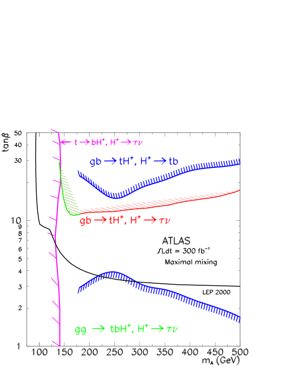
Figure 1: We display the contours for $5\sigma$ charged Higgs detection from [22].

As regards the charged Higgs boson, it is well established (for early studies, see refs. [16, 15]) that if $t\to h^{\pm}b$ decays are kinematically allowed then the $h^{\pm}$ will be relatively easily discovered in the decay of the top quark in $t\overline{t}$ events. These earlier studies have been updated by ATLAS in [22]. The resulting $L=300~{}{\rm fb}^{-1}$ plot appears in fig. 1. The least sensitivity to a charged Higgs boson occurs for $\tan\beta\sim 4\div 10$ where $5\sigma$ is only attained for the MSSM parameter $m_{A}\raise 1.29167pt\hbox{$<$\kern-7.5pt\raise-4.73611pt\hbox{$\sim$}}135~{}{\rm GeV}$, corresponding to $m_{h^{\pm}}\raise 1.29167pt\hbox{$<$\kern-7.5pt\raise-4.73611pt\hbox{$\sim$}}155~{}{\rm GeV}$. Once $m_{h^{\pm}}\raise 1.29167pt\hbox{$>$\kern-7.5pt\raise-4.73611pt\hbox{$\sim$}}210~{}{\rm GeV}$, the Higgs-to-Higgs decay mode $h^{\pm}\to W^{\pm}h_{1}$ is typically kinematically allowed and in the NMSSM can have substantial branching ratio. Thus, in the NMSSM context the limits of fig. 1 on the $h^{\pm}$ in the region $m_{h^{\pm}}\raise 1.29167pt\hbox{$>$\kern-7.5pt\raise-4.73611pt\hbox{$\sim$}}210~{}{\rm GeV}$ do not apply.

We will study the complementarity between charged Higgs detection and neutral Higgs detection in the standard modes 1) – 9). We find that the smaller the lower limit on $m_{h^{\pm}}$ for which we assume good significance for $t\to h^{\pm}b$ detection, the smaller can be the minimum statistical significance for the neutral Higgs detection modes.

In Ref. [4], a partial no-lose theorem for NMSSM Higgs boson discovery at the LHC (when Higgs-to-Higgs decays are forbidden) was established based on modes 1) - 8) above. There, we estimated the statistical significances ($N_{SD}=S/\sqrt{B}$) for modes 1) - 8). For these results, it was especially critical that the $t\overline{t}h$ with $h\to b\overline{b}$ and $WW$-fusion modes [3) and 7), respectively] were included. Also important was mode 4), $b\overline{b}h$ with $h\to\tau^{+}\tau^{-}$. In the case of $t\overline{t}h$ with $h\to b\overline{b}$, we used the experimental study done by V. Drollinger at our request (see the Appendix) that extends results for this mode to Higgs masses as large as $150~{}{\rm GeV}$. The conclusion of ref. [4] was that, for an integrated luminosity of $L=300~{}{\rm fb}^{-1}$ at the LHC, all the surviving points yielded $N_{SD}>10$ after combining all modes. This means that NMSSM Higgs boson discovery by just one detector with $L=300~{}{\rm fb}^{-1}$ is essentially guaranteed for those portions of parameter space for which Higgs boson decays to other Higgs bosons are kinematically forbidden.

For the present paper, we have repeated the scan described above with the latest available LEP constraints (as incorporated in NMHDECAY [9] – see references therein) and with the latest ATLAS and CMS results for the discovery channels 1) – 9) (see the Appendix) and most recent $5\sigma$ curve for the $h^{\pm}$ as given in fig. 1. For each Higgs state, we calculated all branching ratios using NMHDECAY. We then estimated the expected statistical significances at the LHC in all Higgs boson detection modes 1) – 9) by rescaling results for the SM Higgs boson and/or the MSSM $h,H$ and/or $A$. The rescaling factors for the CP-even $h_{i}$ are determined by $R_{i}$, $t_{i}$, $b_{i}=\tau_{i}$, $g_{i}$ and $\gamma_{i}$, the ratios of the $VVh_{i}$, $t\overline{t}h_{i}$, $b\overline{b}h_{i}$ (or $\tau^{+}\tau^{-}h_{i}$), $ggh_{i}$ and $\gamma\gamma h_{i}$ couplings, respectively, to those of a SM Higgs boson of the same mass. Of course $|R_{i}|<1$, but $t_{i}$, $b_{i}$, $g_{i}$ and $\gamma_{i}$ can be larger, smaller or even differ in sign with respect to the SM. The reduced couplings for the CP-odd Higgs bosons (denoted by primes) are as follows: $R_{i}^{\prime}=0$ at tree-level; $t^{\prime}_{j}$ and $b^{\prime}_{j}$ are the ratios of the $i\gamma_{5}$ couplings for $t\bar{t}$ and $b\bar{b}$, respectively, relative to SM-like strength. The quantities $g_{i}^{\prime}$ and $\gamma_{i}^{\prime}$ are the ratios of the $\epsilon\times\epsilon^{\prime}$ ($\epsilon$ and $\epsilon^{\prime}$ being the polarizations of the gluons or photons) $gga_{i}$ or $\gamma\gamma a_{i}$ coupling strength to the $\epsilon\cdot\epsilon^{\prime}$ $ggh_{SM}$ or $\gamma\gamma h_{SM}$ coupling strength for $m_{a_{i}}=m_{h_{SM}}$. A detailed discussion of the procedures for rescaling SM and MSSM simulation results for the statistical significances in channels 1) – 9) is given in the Appendix. We will now summarize the results of this new no-Higgs-to-Higgs scan.

Only a few parameter choices are such that decays of a neutral Higgs boson to any other Higgs boson are all forbidden when $m_{h^{\pm}}\geq 155~{}{\rm GeV}$ is required. After restricting to such parameters, it is extraordinarily difficult to locate points that do not yield large statistical significance for LHC discovery of at least one Higgs boson while at the same time LEP constraints are not violated. We obtained a sample of $2455$ points that had LHC significance (for $L=300~{}{\rm fb}^{-1}$) in channels 1) – 9) below $10\sigma$. Most of these points had $4\raise 1.29167pt\hbox{$<$\kern-7.5pt\raise-4.73611pt\hbox{$\sim$}}\tan\beta\raise 1.29167pt\hbox{$<$\kern-7.5pt\raise-4.73611pt\hbox{$\sim$}}10$ — high $\tan\beta$ enhances production cross sections for some of the Higgs bosons and will typically lead to visible signals. All points had LHC statistical significance above $5\sigma$, thus establishing a no-lose theorem for points chosen consistent with LEP constraints and absence of Higgs-to-Higgs decays. Statistics on the important channels for these $2455$ points are summarized in table 1. Note the importance of the channels 3), 4) and 7) for these most difficult cases.

Channel with highest $S/\sqrt{B}$	1	2	3	4	5	6	7	8	9
No. of points	0	0	343	132	0	1	1979	0	0

Table 1: Most important channel for detecting the $2455$ no-Higgs-to-Higgs-decays points that were most difficult for LHC detection.

In fig. 2, we give a scatter plot of the largest statistical significance achieved for a single neutral Higgs boson, $N_{SD}^{\rm max}$, as a function of $m_{h^{\pm}}$ for the above $2455$ points. (The absence of points with $m_{h^{\pm}}\raise 1.29167pt\hbox{$>$\kern-7.5pt\raise-4.73611pt\hbox{$\sim$}}210~{}{\rm GeV}$ is due to the fact that above this scale Higgs-to-Higgs decays, typically $a_{2}\to Zh_{1}$ and $h^{\pm}\to W^{\pm}h_{1}$, would be allowed.) We see that the larger the value of $m_{h^{\pm}}$ for which a $5\sigma$ signal can be established using $t\overline{t}$ production with $t\to h^{\pm}b$ decay, the larger the minimum possible value of the neutral Higgs bosons’ $N_{SD}^{\rm max}$. This means that the ATLAS and CMS groups should work to maximize sensitivity to charged Higgs production as well as to neutral Higgs production.

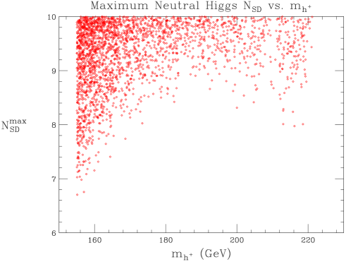
Figure 2: $N_{SD}^{\rm max}$ for the neutral Higgs bosons vs. $m_{h^{\pm}}$ for $m_{h^{\pm}}\geq 155~{}{\rm GeV}$. Here, $N_{SD}^{\rm max}$ is the largest of the significances for any one of the neutral Higgs bosons in channels 1) - 9). We assume LHC luminosity of $L=300~{}{\rm fb}^{-1}$.

The point yielding the very lowest LHC statistical significance had the following parameters,

$$\lambda=0.0163;\quad\kappa=-0.0034;\quad\tan\beta=5.7;$$

$$\mu_{\rm eff}=-284~{}{\rm GeV};\quad A_{\lambda}=-70~{}{\rm GeV};\quad A_{\kappa}=-54~{}{\rm GeV}\,,$$ (8)

which yielded $m_{h^{\pm}}\sim 155~{}{\rm GeV}$ and neutral Higgs boson properties as given in table 2. Other points among the $2455$ are similar in that the Higgs masses are closely spaced and below or at least not far above the $WW/ZZ$ decay thresholds, the CP-even Higgs bosons tend to share the $WW/ZZ$ coupling strength (indicated by $R_{i}$ in the table), couplings to $b\overline{b}$ of all Higgs bosons (the $b_{i}$ or $b_{i}^{\prime}$ in the table) are not very enhanced, and couplings to $gg$ and $\gamma\gamma$ (the $g_{i}$ or $g_{i}^{\prime}$ and $\gamma_{i}$ or $\gamma_{i}^{\prime}$ in the table) are suppressed relative to the SM Higgs strength. The most visible processes for this point had $N_{SD}$ values above $6$. These were the $WW\to h_{2}\to\tau^{+}\tau^{-}$, $WW\to h_{3}\to\tau^{+}\tau^{-}$ and $t\overline{t}h_{2}\to t\overline{t}b\overline{b}$ channels. Overall, we have a quite robust LHC no-lose theorem for NMSSM parameters such that LEP constraints are passed and Higgs-to-Higgs decays are not allowed.

Higgs	$h_{1}$	$h_{2}$	$h_{3}$	$a_{1}$	$a_{2}$
Mass (GeV)	$99$	$114$	$145$	$98$	$134$
$R_{i}$	$0.49$	$0.72$	$-0.48$	$-$	$-$
$t_{i}$ or $t_{i}^{\prime}$	$0.46$	$0.65$	$-0.64$	$-0.01$	$0.18$
$b_{i}$ or $b_{i}^{\prime}$	$1.71$	$3.23$	$4.49$	$0.36$	$5.59$
$g_{i}$ or $g_{i}^{\prime}$	$0.41$	$0.56$	$0.79$	$0.02$	$0.14$
$\gamma_{i}$ or $\gamma_{i}^{\prime}$	$0.51$	$0.75$	$0.43$	$0.01$	$0.10$
$BR(h_{i}~{}or~{}a_{i}\to b\overline{b})$	$0.91$	$0.90$	$0.88$	$0.92$	$0.91$
$BR(h_{i}~{}or~{}a_{i}\to\tau^{+}\tau^{-})$	$0.08$	$0.08$	$0.09$	$0.08$	$0.09$
Chan. 1) $S/\sqrt{B}$	0.00	0.22	0.20	0.00	0.00
Chan. 2) $S/\sqrt{B}$	0.42	0.80	0.15	0.42	0.00
Chan. 3) $S/\sqrt{B}$	3.52	6.25	5.39	3.52	5.39
Chan. 4) $S/\sqrt{B}$	0.73	1.26	3.86	1.26	3.86
Chan. 5) $S/\sqrt{B}$	0.00	0.15	1.00	$-$	$-$
Chan. 6) $S/\sqrt{B}$	0.00	0.00	0.80	$-$	$-$
Chan. 7) $S/\sqrt{B}$	0.00	6.70	6.54	$-$	$-$
Chan. 8) $S/\sqrt{B}$	0.00	0.20	0.25	$-$	$-$
All-channel $S/\sqrt{B}$	3.61	9.29	9.41	3.76	6.63

Table 2: Properties of the neutral NMSSM Higgs bosons for the most difficult no-Higgs-to-Higgs-decays LHC point. In the table, $R_{i}=g_{h_{i}VV}/g_{h_{SM}VV}$, $t_{i}=g_{h_{i}t\overline{t}}/g_{h_{SM}t\overline{t}}$, $b_{i}=g_{h_{i}b\overline{b}}/g_{h_{SM}b\overline{b}}$, $g_{i}=g_{h_{i}gg}/g_{h_{SM}gg}$ and $\gamma_{i}=g_{h_{i}\gamma\gamma}/g_{h_{SM}\gamma\gamma}$ for $m_{h_{SM}}=m_{h_{i}}$. Similarly, $t_{i}^{\prime}$ and $b_{i}^{\prime}$ are the $i\gamma_{5}$ couplings of $a_{i}$ to $t\overline{t}$ and $b\overline{b}$ normalized relative to the scalar $t\overline{t}$ and $b\overline{b}$ SM Higgs couplings and $g_{i}^{\prime}$ and $\gamma_{i}^{\prime}$ are the $a_{i}gg$ and $a_{i}\gamma\gamma$ $\epsilon\times\epsilon^{\prime}$ couplings relative to the $\epsilon\cdot\epsilon^{\prime}$ coupling of the SM Higgs.

Higgs	$h_{1}$	$h_{2}$	$h_{3}$	$a_{1}$	$a_{2}$
Mass (GeV)	$113.$	$126.$	$203.$	$150.$	$202.$
$R_{i}$	$0.75$	$0.66$	$0.01$	$-$	$-$
$t_{i}$ or $t_{i}^{\prime}$	$0.74$	$0.65$	$0.22$	$-0.01$	$0.12$
$b_{i}$ or $b_{i}^{\prime}$	$1.38$	$1.18$	$-8.11$	$-0.78$	$8.22$
$g_{i}$ or $g_{i}^{\prime}$	$0.72$	$0.63$	$0.37$	$0.01$	$0.08$
$\gamma_{i}$ or $\gamma_{i}^{\prime}$	$0.76$	$0.65$	$0.93$	$0.06$	$0.05$
$BR(h_{i}~{}or~{}a_{i}\to b\overline{b})$	$0.87$	$0.80$	$0.86$	$0.91$	$0.90$
$BR(h_{i}~{}or~{}a_{i}\to\tau^{+}\tau^{-})$	$0.08$	$0.08$	$0.09$	$0.09$	$0.10$
Chan. 1) $S/\sqrt{B}$	1.91	2.05	0.00	0.00	0.00
Chan. 2) $S/\sqrt{B}$	4.99	4.02	0.00	0.00	0.00
Chan. 3) $S/\sqrt{B}$	7.84	5.95	0.00	0.00	0.00
Chan. 4) $S/\sqrt{B}$	0.20	0.20	7.40	0.05	7.40
Chan. 5) $S/\sqrt{B}$	1.33	2.84	0.31	$-$	$-$
Chan. 6) $S/\sqrt{B}$	0.00	2.23	0.19	$-$	$-$
Chan. 7) $S/\sqrt{B}$	6.67	7.62	0.00	$-$	$-$
Chan. 8) $S/\sqrt{B}$	1.14	3.85	0.00	$-$	$-$
All-channel $S/\sqrt{B}$	11.73	11.91	7.41	0.05	7.40

Table 3: Properties of the neutral NMSSM Higgs bosons for the second interesting point described in the text. Notation as in table 2.

Another example point of possible interest is that giving the weakest signals when the charged Higgs mass is near the upper end of the spectrum for which the $h^{\pm}$ does not decay to other Higgs bosons. (This requirement is what restricts the upper range of $m_{h^{\pm}}$ in fig. 2.) The parameters for this point are:

$$\lambda=0.0379;\quad\kappa=-0.0238;\quad\tan\beta=8.25;$$

$$\mu_{\rm eff}=-119~{}{\rm GeV};\quad A_{\lambda}=-116~{}{\rm GeV};\quad A_{\kappa}=-102~{}{\rm GeV}\,,$$ (9)

yielding a charged Higgs mass of $216~{}{\rm GeV}$ and neutral Higgs properties and statistical significances as listed in table 3. Note the strong signals in the $WW\to h_{1,2}\to\tau^{+}\tau^{-}$, $t\overline{t}h_{1,2}\to t\overline{t}b\overline{b}$ and $b\overline{b}h_{3},a_{2}\to b\overline{b}\tau^{+}\tau^{-}$ channels.

These particular points in parameter space illustrate the general conclusion that it will be important that all the neutral Higgs detection modes that have been simulated by ATLAS and CMS really achieve their full $L=300~{}{\rm fb}^{-1}$ potential. If the effective luminosity accumulated in modes 3), 4) and 7) were to all fall below $L\sim 100~{}{\rm fb}^{-1}$, then all single channel statistical significances for the most marginal points (as exemplified by the two tabulated points) would fall below $5\sigma$. Channel combination would be required to reach the $\geq 5\sigma$ level.

4 LHC prospects when Higgs-to-Higgs decays are allowed

In this section we will consider the part of the parameter space complementary to that scanned in section 3. To be precise, we require that at least one of the following decay modes be kinematically allowed for some $h$ and or $a$:

$$i)\ h\to h^{\prime}h^{\prime}\;,\quad ii)\ h\to aa\;,\quad iii)\ h\to h^{\pm}h^{\mp}\;,\quad iv)\ h\to aZ\;,$$

$$v)\ h\to h^{\pm}W^{\mp}\;,\quad vi)\ a^{\prime}\to ha\;,\quad vii)\ a\to hZ\;,\quad viii)\ a\to h^{\pm}W^{\mp}\;.$$ (10)

(Recall that we do not consider $h^{\pm}\to W^{\pm}h$ or $h^{\pm}\to W^{\pm}a$ in defining the Higgs-to-Higgs decay parameter region.) The branching ratios for all these decays are computed by NMHDECAY. As in the previous section, we also allow for (but do not require) Higgs decays to gauginos. The large gaugino masses we employ imply that such decays are never important for the scans discussed in this paper.

For most of these points it turns out that $5\sigma$ discovery of a neutral Higgs boson in at least one of the modes 1) – 9) is still possible. The number of parameter space points for which one or more of the decays $i)-viii)$ is allowed, but $5\sigma$ discovery of a neutral Higgs boson in modes 1) – 9) is not possible, represents less than $1\%$ of the physically acceptable points; in our scan we have found $3480$ such points. In one sense, this small percentage is encouraging in that it implies that the standard LHC detection modes 1) – 9) suffice for most of randomly chosen parameter points. However, it should be noted that the fraction of points for which modes 1) – 9) suffice will decrease rapidly as the assumed LHC integrated luminosity is reduced. Further, the difficult parameter points are preferred on the basis of keeping fine-tuning modest in size [3]. (Modest fine-tuning means that $m_{Z}$ is not very sensitive to GUT scale choices for the soft-Susy-breaking parameters.)

The parameters associated with these points for which all NMSSM Higgs bosons escape LEP detection and LHC detection in modes 1) – 9) occur throughout the broad range defined in eq. (6). The scenarios associated with these points have some generic properties of considerable interest that make them worthy of further study. First, for all these $3480$ points, the $h_{3}$ and $a_{2}$ are so heavy that they will only be detectable if a super high energy LC is eventually built so that $e^{+}e^{-}\to Z\to h_{3}a_{2}$ is possible, implying that LHC Higgs detection must rely on the lighter $h_{1}$, $h_{2}$ and $a_{1}$ states. The NMSSM parameter choices for which the latter cannot be detected at the LHC in the standard modes are such that there is a light, fairly SM-like CP-even Higgs boson ($h_{1}$ or $h_{2}$) that decays mainly to two lighter CP-odd or CP-even Higgs bosons ($h_{1,2}\to a_{1}a_{1}$ or $h_{2}\to h_{1}h_{1}$). We will denote the parent SM-like CP-even Higgs boson by $h_{H}$ and the daughter Higgs boson that appears in the pair decay by $h_{L}$.

We should discuss how it is that a light $h_{L}$ will have escaped LEP detection. Consider the case of $h_{L}=a_{1}$. First, sum rules require that the $Zh_{1}a_{1}$ ($Zh_{2}a_{1}$) coupling is small when the $h_{1}$ ($h_{2}$) coupling is near SM strength, implying that discovery in the $e^{+}e^{-}\to Z^{*}\to h_{1}a_{1}$ ($e^{+}e^{-}\to Z^{*}\to h_{2}a_{1}$) mode will not be possible. Second, $e^{+}e^{-}\to Z^{*}\to h_{2}a_{1}$ ($h_{1}a_{1}$) LEP constraints can be evaded in the NMSSM since the $a_{1}$ can have sufficient singlet component that the $Zh_{2}a_{1}$ ($Zh_{1}a_{1}$) coupling is small when the $h_{1}$ ($h_{2}$) is SM-like. For scenarios in which the $h_{2}$ is SM-like and decays primarily via $h_{2}\to h_{1}h_{1}$, the $h_{1}$ is not observed at LEP because of its weak $ZZ$ coupling, while the $h_{2}$ mass is beyond the reach of LEP.

As we review the properties of specific bench mark points, it is useful to keep in mind the fact that detection of Higgs-pair final states at the LHC might be possible in certain cases. In particular, in  [6, 7] we proposed that the LHC may be able to detect Higgs-pair final states using the $WW\to h_{H}\to h_{L}h_{L}\to jj\tau^{+}\tau^{-}$ production/decay mode. By this we mean that one of the final $h_{L}$ Higgs bosons is required to decay to a $\tau^{+}\tau^{-}$ pair where we identify the $\tau$’s through their leptonic decays to electrons and muons. The other final $h_{L}$ is required to decay to either $b\overline{b}$ (which we identify as jets) or, if $b\overline{b}$ is not a kinematically allowed decay, to $jj$ or (with much smaller identification efficiency) $\tau^{+}\tau^{-}$ where the $\tau$’s of this second pair would be tagged via their decays to single jets plus neutrinos. However, for a small fraction of the $3480$ points, $h_{H}\to a_{1}a_{1}$ decays are prominent but $m_{a_{1}}\leq 2m_{\tau}$. For another small fraction, the $h_{L}$ has suppressed couplings to $b\overline{b}$ and $\tau^{+}\tau^{-}$. In either case, $\tau$ triggering does not work and NMSSM Higgs detection at the LHC would probably be impossible. We will discuss this more in section 5.

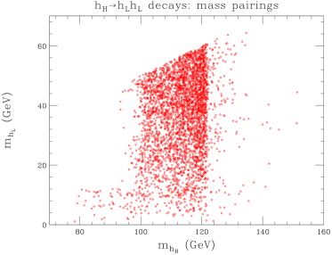
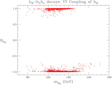
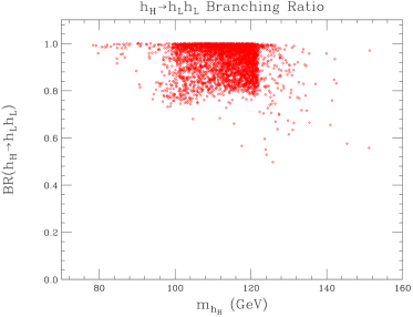
Figure 3: The top, middle and bottom plots give a scatter plot of $m_{h_{L}}$, $R_{h_{H}}$ and $BR(h_{H}\to h_{L}h_{L})$, respectively, versus $m_{h_{H}}$ for the $3480$ sample scan points with $h_{H}\to h_{L}h_{L}$ decays.

The distribution of the mass of the heavier SM-like Higgs ($h_{H}$, where $h_{H}=h_{1}$ or $h_{2}$) as compared to the mass of the lighter Higgs ($h_{L}$, where $h_{L}=a_{1}$ or $h_{1}$) appearing in the $h_{H}\to h_{L}h_{L}$ decay for the $3480$ points from the scan described above is given in the top plot of fig. 3. We see that the SM-like parent Higgs mass $m_{h_{H}}$ lies in the $[75~{}{\rm GeV},155~{}{\rm GeV}]$ interval while daughter Higgs masses $m_{h_{L}}$ range from near $0$ up to close to $m_{h_{H}}/2$. The middle plot of fig. 3 shows that the parent $h_{H}$ always has fairly SM-like coupling $|R_{h_{H}}|\geq 0.7$ to vector bosons; for most of the points, $|R_{h_{H}}|$ is quite close to $1$. The bottom plot of fig. 3 shows that for these points $BR(h_{H}\to h_{L}h_{L})$ is always substantial. The importance of the $WW\to h_{H}\to h_{L}h_{L}$ discovery mode is thus evident.

Out of the above $3480$ points, we have selected eight benchmark points, the properties of which are displayed in tables 4 and 5, that illustrate the cases where LHC detection of the NMSSM Higgs bosons in the standard modes 1) – 9) would not be possible. The first five are such that the $WW\to h_{H}\to h_{L}h_{L}\to jj\tau^{+}\tau^{-}$ detection mode might be effective. Points 6, 7 and 8 are chosen to illustrate cases where the $h_{L}$ appearing in the final state does not decay to either $b\overline{b}$ or $\tau^{+}\tau^{-}$, implying that the $WW\to h_{H}\to h_{L}h_{L}\to jj\tau^{+}\tau^{-}$ potential detection mode would not be useful.

We now discuss in more detail the characteristics of these eight benchmark points.

• Points 1, 2 and 3 are designed to illustrate $h_{1}\to a_{1}a_{1}$ decay cases for a selection of possible $h_{1}$ and $a_{1}$ masses.
  Point 1 is in the low-mass tail of the $h_{H}$ mass distribution (see fig. 3) at $90~{}{\rm GeV}$ (although $m_{h_{H}}$ as lows a $80~{}{\rm GeV}$ is possible). For point 1, $m_{a_{1}}$ is below the $b\overline{b}$ threshold so that the main $a_{1}$ decay is to $\tau^{+}\tau^{-}$ or $jj$.
  Point 2 and point 3 are at the two extremes of the central bulk of the $h_{H}$ mass distribution of fig. 3 with $m_{h_{H}}=100~{}{\rm GeV}$ and $120~{}{\rm GeV}$, respectively. For these latter two points $m_{a_{1}}$ is $20~{}{\rm GeV}$ or $30~{}{\rm GeV}$; $a_{1}\to b\overline{b}$ and $a_{1}\to\tau^{+}\tau^{-}$ decays will be dominant and in the usual ratio.

• Point 4 is such that the $h_{1}$ and $h_{2}$ (with masses $m_{h_{1}}=97~{}{\rm GeV}$ and $m_{h_{2}}=150~{}{\rm GeV}$) share the $WW/ZZ$ coupling strength squared and both decay to $a_{1}a_{1}$. The $a_{1}$ decays to $b\overline{b}$ and $\tau^{+}\tau^{-}$ in the usual ratio. Note that this point is an example for which $m_{a_{1}}$ is fairly large ($m_{a_{1}}=45~{}{\rm GeV}$).

• Point 5 illustrates a case in which it is the $h_{2}$ that is SM-like and it decays to $h_{1}h_{1}$. The $h_{1}\to b\overline{b}$ and $h_{1}\to\tau^{+}\tau^{-}$ decays are the dominant ones and are in the usual ratio. Although $m_{h_{1}}$ is rather small in this case, it would not have been seen at LEP due to its singlet nature. Nonetheless, $BR(h_{2}\to h_{1}h_{1})$ is large due to the new trilinear NMSSM couplings.

• For point 6, the $h_{1}$ is SM-like and decays via $h_{1}\to a_{1}a_{1}$, but $a_{1}\to\gamma\gamma$ is dominant due to the singlet nature of $a_{1}$. The $4\gamma$ final state would provide a highly distinctive signal that should be easily seen at the LHC [14].

• Point 7 illustrates a case in which the $h_{2}$ is SM-like and decays via $h_{2}\to h_{1}h_{1}$. The new feature compared to point 5 is that the $h_{1}$ has reduced coupling to $b\overline{b}$ and $\tau^{+}\tau^{-}$ due to the fact that parameters are such that $h_{1}$ is almost entirely $H_{u}$ in nature [8]. Obviously, the $WW\to h_{2}\to jj\tau^{+}\tau^{-}$ mode would not be relevant for this type of scenario. We do not think that the resulting $h_{2}\to 4j$ signal could be isolated from backgrounds.

• Point 8 illustrates a case in which the $h_{1}$ is SM-like and decays via $h_{1}\to a_{1}a_{1}$. It differs from earlier such points in that the $a_{1}$ is extremely light and decays mainly to $jj$ ($j=s,c,g$). Like for point 7, the $WW\to h_{1}\to jj\tau^{+}\tau^{-}$ detection channel would not be relevant. We would need to isolate a $h_{1}\to 4j$ signal within a large QCD background. We do not believe this will be possible, especially given that each of the pairs of jets will have small mass and large boost, making separation of the two jets within each pair very problematical.
  This $a_{1}$ would not have been seen at LEP in the $h_{1}a_{1}$ mode for several reasons (for details see the references and discussions in [9]):

  1. First, the $Zh_{1}a_{1}$ coupling is very small because of the very SM-like nature of the $h_{1}$.

  2. Second, $m_{a_{1}}$ is below the threshold of any existing study of the $ha$ type of mode at LEP.

  3. Third, the existing $Zh_{1}\to Za_{1}a_{1}$ limits (from OPAL) for the case where $a_{1}\to jj$ do not cover the mass regions corresponding to the values of either $m_{h_{1}}$ or $m_{a_{1}}$. In fact, they extend only up to $m_{h_{1}}\sim 90~{}{\rm GeV}$ and in any case do not apply when $m_{a_{1}}$ is below the $2~{}{\rm GeV}$ threshold for their searches.

  Finally, we note that axion searches do not apply since the $a_{1}$ would not have been invisible in the detector — it decays promptly to visible jets.

Point Number	1	2	3	4	5
Bare Parameters
$\lambda$	$0.22$	$0.4$	$0.22$	$0.67$	$0.56$
$\kappa$	$-0.1$	$-0.35$	$0.59$	$0.2$	$0.1$
$\tan\beta$	$5.$	$15.$	$7.8$	$4.1$	$2.5$
$\mu_{\rm eff}$ (GeV)	$-520.$	$-160.$	$530.$	$-200.$	$-180.$
$A_{\lambda}$ (GeV)	$-580.$	$-580.$	$-920.$	$-600.$	$-440.$
$A_{\kappa}$ (GeV)	$-2.8$	$-8.7$	$-2.1$	$-30.$	$172.$
CP-even Higgs Boson Masses and Couplings
$m_{h_{1}}$ (GeV)	$90.$	$100.$	$119.$	$97.$	$40.$
$R_{1}$	$0.99$	$0.97$	$-1.00$	$0.69$	$0.00$
$t_{1}$	$0.99$	$0.97$	$-1.00$	$0.72$	$0.05$
$b_{1}$	$1.00$	$0.90$	$-1.01$	$0.31$	$-0.35$
$g_{1}$	$0.99$	$0.97$	$1.00$	$0.74$	$0.15$
$\gamma_{1}$	$0.99$	$0.99$	$1.00$	$0.78$	$0.11$
$BR(h_{1}\to b\overline{b})$	$0.08$	$0.02$	$0.01$	$0.01$	$0.93$
$BR(h_{1}\to\tau^{+}\tau^{-})$	$0.01$	$0.00$	$0.00$	$0.00$	$0.07$
$BR(h_{1}\to a_{1}a_{1})$	$0.91$	$0.97$	$0.99$	$0.99$	$0.00$
$m_{h_{2}}$ (GeV)	$479.$	$288.$	$1431.$	$150.$	$125.$
$R_{2}$	$0.16$	$0.26$	$0.00$	$0.72$	$-1.00$
$t_{2}$	$0.16$	$0.26$	$0.13$	$0.70$	$-1.00$
$b_{2}$	$0.19$	$0.57$	$-7.8$	$1.10$	$-1.03$
$g_{2}$	$0.16$	$0.26$	$0.12$	$0.69$	$0.99$
$\gamma_{2}$	$0.19$	$0.24$	$0.08$	$0.65$	$0.99$
$BR(h_{2}\to a_{1}a_{1})$	$0.04$	$0.44$	$0.00$	$0.97$	$0.00$
$BR(h_{2}\to h_{1}h_{1})$	$0.25$	$0.21$	$0.00$	$0.00$	$0.92$
$m_{h_{3}}$ (GeV)	$952.$	$1016.$	$2842.$	$753.$	$495.$
CP-odd Higgs Boson Masses and Couplings
$m_{a_{1}}$ (GeV)	$10.$	$20.$	$31.$	$45.$	$144.$
$t_{1}^{\prime}$	$-0.01$	$0.00$	$-0.01$	$-0.02$	$-0.06$
$b_{1}^{\prime}$	$-0.22$	$-0.85$	$-0.53$	$-0.40$	$-0.40$
$g_{1}^{\prime}$	$0.15$	$0.48$	$0.19$	$0.08$	$0.06$
$\gamma_{1}^{\prime}$	$0.12$	$0.11$	$0.15$	$0.49$	$0.61$
$BR(a_{1}\to b\overline{b})$	$0.00$	$0.94$	$0.93$	$0.93$	$0.85$
$BR(a_{1}\to\tau^{+}\tau^{-})$	$0.83$	$0.06$	$0.07$	$0.07$	$0.08$
$BR(a_{1}\to jj)$	$0.17$	$0.00$	$0.00$	$0.00$	$0.01$
$m_{a_{2}}$ (GeV)	$952.$	$1018.$	$1434.$	$750.$	$495.$
Charged Higgs Boson Mass
$m_{h^{\pm}}$ (GeV)	$954.$	$1017.$	$1432.$	$742.$	$487.$
LSP Mass
$m_{\widetilde{\chi}_{1}^{0}}$	$453.$	$136.$	$476.$	$113.$	$82.$
Most Visible of the LHC Processes 1)-9)	2($h_{1}$)	5($h_{2}$)	2($h_{1}$)	5($h_{2}$)	2($h_{2}$)
$N_{SD}=S/\sqrt{B}$ of this process at $L=$300 ${\rm fb}^{-1}$	$1.6$	$0.7$	$0.3$	$0.5$	$2.0$

Table 4: Properties of five scenarios for which LHC Higgs detection would only be possible in the $WW\to h_{1,2}\to a_{1}a_{1}\to jj\tau^{+}\tau^{-}$ or $WW\to h_{2}\to h_{1}h_{1}\to jj\tau^{+}\tau^{-}$ mode. The quantities $R_{i}$, $t_{i}$, $b_{i}$, $g_{i}$, $\gamma_{i}$, $t_{i}^{\prime}$, $b_{i}^{\prime}$, $g_{i}^{\prime}$ and $\gamma_{i}^{\prime}$ were defined in the caption of table 2. Important absolute branching ratios are displayed. Only the masses of the heavy $h_{3}$, $a_{2}$ and $h^{\pm}$ are given. The mass of the lightest neutralino (LSP) is also given. The second-to-last row gives the channel and Higgs boson yielding the largest $N_{SD}=S/\sqrt{B}$ in channels 1) – 9). The following row gives the corresponding $N_{SD}$ for $L=300~{}{\rm fb}^{-1}$.

Point Number	6	7	8
Bare Parameters
$\lambda$	$0.39$	$0.5$	$0.27$
$\kappa$	$0.18$	$-0.15$	$0.15$
$\tan\beta$	$3.5$	$3.5$	$2.9$
$\mu_{\rm eff}$	$-245.$	$200.$	$-753.$
$A_{\lambda}$	$-230.$	$780.$	$312.$
$A_{\kappa}$	$-5.$	$230.$	$8.4$
CP-even Higgs Boson Masses and Couplings
$m_{h_{1}}$ (GeV)	$94.$	$57.$	$95.$
$R_{1}$	$0.94$	$-0.28$	$1.00$
$t_{1}$	$0.95$	$-0.30$	$0.99$
$b_{1}$	$0.89$	$0.01$	$1.05$
$g_{1}$	$0.95$	$0.33$	$0.99$
$\gamma_{1}$	$0.96$	$0.37$	$1.00$
$BR(h_{1}\to jj)$	$0.01$	$0.93$	$0.00$
$BR(h_{1}\to a_{1}a_{1})$	$0.94$	$0.00$	$1.00$
$m_{h_{2}}$ (GeV)	$239.$	$125.$	$483.$
$R_{2}$	$0.33$	$-0.96$	$-0.01$
$t_{2}$	$0.30$	$-0.95$	$-0.36$
$b_{2}$	$0.67$	$-1.07$	$2.84$
$g_{2}$	$0.29$	$0.95$	$0.37$
$\gamma_{2}$	$0.30$	$0.94$	$0.68$
$BR(h_{2}\to h_{1}h_{1})$	$0.32$	$0.93$	$0.01$
$m_{h_{3}}$ (GeV)	$562.$	$731.$	$821.$
CP-odd Higgs Boson Masses and Couplings
$m_{a_{1}}$ (GeV)	$40.$	$188.$	$1.$
$t_{1}^{\prime}$	$0.00$	$0.04$	$0.08$
$b_{1}^{\prime}$	$0.00$	$0.53$	$0.62$
$g_{1}^{\prime}$	$0.00$	$0.04$	$0.36$
$\gamma_{1}^{\prime}$	$0.47$	$0.31$	$0.39$
$BR(a_{1}\to jj)$	$0.00$	$0.00$	$0.95$
$BR(a_{1}\to\mu\mu)$	$0.00$	$0.00$	$0.05$
$BR(a_{1}\to\gamma\gamma)$	$0.98$	$0.00$	$0.00$
$BR(a_{1}\to\widetilde{\chi}_{1}^{0}\widetilde{\chi}_{1}^{0})$	$0.00$	$0.99$	$0.00$
$m_{a_{2}}$ (GeV)	$558.$	$736.$	$493.$
Charged Higgs Boson Mass
$m_{h^{\pm}}$ (GeV)	$560.$	$727.$	$485.$
LSP Mass
$m_{\widetilde{\chi}_{1}^{0}}$	$211.$	$81.$	$500.$
Most Visible of the LHC Processes 1)-9)	5($h_{2}$)	2($h_{2}$)	5($h_{3}$)
$N_{SD}=S/\sqrt{B}$ of this process at $L=$300 ${\rm fb}^{-1}$	$1.5$	$1.3$	$0.1$

Table 5: Properties of three representative scenarios for which LHC Higgs detection would not even be possible in the $WW\to h_{1,2}\to a_{1}a_{1}\to jj\tau^{+}\tau^{-}$ or $WW\to h_{2}\to h_{1}h_{1}\to jj\tau^{+}\tau^{-}$ modes.

5 Collider Implications

In the previous section, we have established the probable importance and possible necessity of detecting a fairly SM-like, relatively light Higgs boson, $h_{H}$, in a Higgs-pair decay mode, $h_{H}\to h_{L}h_{L}$. In this section, we discuss possible ways in which such detection might be possible at various different kinds of colliders, with some emphasis on the LHC. The best means for such detection at hadron colliders will depend strongly upon the $h_{L}$ decay channels. Detection of the $h_{H}$ in the Higgs-pair final state at an $e^{+}e^{-}$ or $\gamma\gamma$ collider will be less dependent upon precisely how the $h_{L}$ decays.

The LHC

At the LHC it will presumably be highly advantageous to use $WW$ fusion production for the $h_{H}$. Not only is the associated production cross section quite competitive with other production mechanisms for $h_{H}$ in the $m_{h_{H}}\in[80~{}{\rm GeV},150~{}{\rm GeV}]$ mass range of relevance, but also the ability to tag the spectator jets will certainly make backgrounds much more manageable.

When $m_{h_{L}}>2m_{b}$, we advocate employing the $h_{L}h_{L}\to b\overline{b}\tau^{+}\tau^{-}$ final state. In this final state an approximate mass for the $h_{H}$ can be computed using the visible particles in the final state to compute an effective mass, $M_{jj\tau^{+}\tau^{-}}$. In addition, restrictions on the visible mass of each $h_{L}$ can also be imposed. (In the analysis, one will need to choose a hypothetical value for $m_{h_{L}}$ and examine the $M_{jj\tau^{+}\tau^{-}}$ mass distribution for a peak. This process will have to be repeated for all possible $m_{h_{L}}$ values. Only the choice with $m_{h_{L}}$ near the actual value would reveal a peak in $M_{jj\tau^{+}\tau^{-}}$.) For the $b\overline{b}\tau^{+}\tau^{-}$ final state, the two main backgrounds appear to be: (i) $gg\to t\overline{t}\to b\overline{b}W^{+}W^{-}\to b\overline{b}\tau^{+}\tau^{-}+\hbox to0.0pt{\hbox to7.95831pt{\hfil/\hfil}\hss}E_{T}$, in association with forward and backward jet radiation and (ii) Drell-Yan $\tau^{+}\tau^{-}+jets$ production. Monte Carlo simulations performed to date show that $b$-tagging does not seem to be necessary to overcome the a priori large Drell-Yan $\tau^{+}\tau^{-}+jets$ background. It is eliminated by stringent cuts for finding the highly energetic forward / backward jets characteristic of the $WW$ fusion process. To the extent that the main background will then come from $t\overline{t}$ production, it is not useful to specifically $b$-tag the $b$ jets since the $t\overline{t}$ background will also contain $b$ jets. Thus, it is appropriate to focus on a generic $WW\to jj\tau^{+}\tau^{-}+\hbox to0.0pt{\hbox to7.95831pt{\hfil/\hfil}\hss}E_{T}$ final state. Such a final state can be experimentally isolated with high efficiency by identifying two $\tau$’s from one $a_{1}$ using the leptonic decay modes for both $\tau$’s while requiring two ($b$) jets from the other $a_{1}$. All these particles should be required to be quite central.

If $m_{h_{L}}<2m_{b}$, but above $2m_{\tau}$, the dominant final state is $h_{L}h_{L}\to\tau^{+}\tau^{-}\tau^{+}\tau^{-}$. However, an effective $h_{H}$ mass is very difficult to reconstruct in this channel. Previous work suggests that it will be best to employ the $h_{L}h_{L}\to jj\tau^{+}\tau^{-}$ final state (which typically has a small but usable branching ratio) where one of the $h_{L}$’s decays to $jj=c\overline{c}$, $s\overline{s}$ or $gg$. This is extracted experimentally by again identifying two $\tau$’s in their leptonic decay modes and two jets.

Preliminary simulations for the $jj\tau^{+}\tau^{-}$ signal have appeared in [6, 7] for a few representative benchmark points (different from those appearing in the tables of this paper). Aside from imposing stringent forward / backward jet tagging cuts to eliminate the Drell-Yan $\tau^{+}\tau^{-}+jets$ background, it was required that the two additional jets (from one of the $h_{L}$’s) and the two opposite sign central leptons ($\ell=e,\mu$) coming from the the $\tau^{+}\tau^{-}$ emerging from the decay of the other $h_{L}$ all be quite central. Additional observations are the following:

• In the case of $m_{h_{L}}>2m_{b}$, the $jj$ mass is fairly high, efficiencies for identifying such $j$’s were found to be high and the momenta of each $j$ were relatively well determined. The latter implies that the $\tau^{+}\tau^{-}$ mass can be reconstructed by assuming that all missing transverse momentum is to be associated with the neutrinos in the $\tau^{+}\tau^{-}\to\ell^{+}\ell^{-}+\nu^{\prime}s$ decays. Efficiencies for the overall reconstruction of this kind of event are therefore reasonably high.

• In the case of $2m_{\tau}<m_{h_{L}}<2m_{b}$, the primary source of the $jj$ is from $c\overline{c}+s\overline{s}+gg$ decays of one of the $h_{L}$’s (neglecting the inefficiently tagged and poorly reconstructed contribution coming from $h_{L}\to\tau^{+}\tau^{-}$ with two $\tau\to j+\hbox to0.0pt{\hbox to7.95831pt{\hfil/\hfil}\hss}E_{T}$ decays, where the $j$ is a single pion or similar hadronic resonance). However, the $jj$ pair mass is quite low ($<2m_{b}$) and separate identification of the two jets was found to be rather inefficient.

  For this case, the relevant final state branching ratio is $BR(h_{L}h_{L}\to jj\tau^{+}\tau^{-})=2\times BR(h_{L}\to c\overline{c}+s\overline{s}+gg)\ BR(h_{L}\to\tau^{+}\tau^{-})$, which is similar in size (typically) for $2m_{\tau}<m_{h_{L}}<2m_{b}$ to what one finds when $m_{h_{L}}>2m_{b}$ for $BR(h_{L}h_{L}\to b\overline{b}\tau^{+}\tau^{-})$.

We reiterate that since the $h_{L}$ will not have been detected previously, we must assume a value for $m_{h_{L}}$ to perform the analysis. We then look among the central jets for the combination with invariant mass $M_{jj}$ closest to $m_{h_{L}}$ (no $b$-tagging is enforced, $b$’s are identified as non-forward/backward jets). We then compute the $M_{jj\tau^{+}\tau^{-}}$ invariant mass using the four reconstructed four-momenta for the two $j$’s and two $\tau$’s and look for a bump in the distribution. This process is repeated for densely spaced $m_{h_{L}}$ values and we look for the $m_{h_{L}}$ choice that produces the best signal.

In our earlier simulations of points with $m_{h_{H}}\in[115~{}{\rm GeV},130~{}{\rm GeV}]$, the typical result found (for the assumed $m_{h_{L}}$ chosen to agree with the actual $m_{h_{L}}$) was a sizable bump in $M_{jj\tau^{+}\tau^{-}}$ coming from the signal in the $M_{jj\tau^{+}\tau^{-}}$ range from roughly $40~{}{\rm GeV}$ to $130~{}{\rm GeV}$. The $t\overline{t}$ background produces a huge peak in $M_{jj\tau^{+}\tau^{-}}$ at high mass with a rapidly falling tail in the $M_{jj\tau^{+}\tau^{-}}\raise 1.29167pt\hbox{$<$\kern-7.5pt\raise-4.73611pt\hbox{$\sim$}}120~{}{\rm GeV}$ region. The crucial issue is the precise shape of this tail and exactly how it extends into the low-$M_{jj\tau^{+}\tau^{-}}$ region where the signal peak resides. The early results of  [6, 7], based on UA1 detector resolutions and efficiencies, found that the low-$M_{jj\tau^{+}\tau^{-}}$ tail from $t\overline{t}$ does not overlap significantly the signal bump, which (for $L=300~{}{\rm fb}^{-1}$) typically contained between 500 and 2000 events in $M_{jj\tau^{+}\tau^{-}}\in[40~{}{\rm GeV},130~{}{\rm GeV}]$. More recently, members of the ATLAS collaboration [24] have examined the $M_{jj\tau^{+}\tau^{-}}$ signal using the ATLAS simulation programs and somewhat different cuts. They find that the $t\overline{t}$ background extends over the full range where the signal resides. This question is now being examined using full simulations in the context of the ATLAS detector and improved cuts [24, 25]. We are unable at this time to say whether or not the signal will emerge above the background in a statistically significant and reliable way.

In principle, one could explore final states other than the $h_{L}h_{L}\to jj\tau^{+}\tau^{-}$ mode. However, all other channels will be much more problematical at the LHC. A $4b$-signal would be present for $m_{h_{L}}>2m_{b}$ but would be burdened by a large QCD background even after implementing $b$-tagging. Meanwhile, for $2m_{\tau}<m_{h_{L}}<2m_{b}$ the $4\tau$-channel would typically have a large branching ratio and we could look for it in the mode where all $\tau$’s decay leptonically. However, in this mode it would not be possible to reconstruct the $h_{H}$ resonance mass and backgrounds would be large.

It should be clear that without the ability to tag one $\tau^{+}\tau^{-}$ pair as part of the $h_{H}$ reconstruction process, the background would be much larger. Thus, it is only for $m_{h_{L}}>2m_{\tau}$ that there is a possibility to isolate the $WW\to h_{H}\to h_{L}h_{L}$ signal. We are very pessimistic regarding isolating a significant signal in a $4j$ final state as appropriate when $m_{h_{L}}<2m_{\tau}$ or in those special cases where $m_{h_{L}}>2m_{\tau}$ but $h_{L}\to jj$ ($j=c,s,g$) decays are dominant.

The Tevatron

At the Tevatron, $WW\to h_{H}$ production has a rather low cross section. Only the $gg\to h_{H}$ cross section is sizable (of order $1~{}{\rm pb}$ for a SM-like $h_{H}$ with $m_{h_{H}}\sim 100~{}{\rm GeV}$). For the case of $m_{h_{L}}>2m_{b}$, one would again employ the $h_{L}h_{L}\to b\overline{b}\tau^{+}\tau^{-}$ final state. However, forward / backward jet tagging could no longer be used to reduce the Drell-Yan $\tau^{+}\tau^{-}+jets$ background without also severely affecting the $gg$ fusion signal. The best means for discriminating against the DY background would probably be to use $b$-tagging. Of course, this will not reduce the dominant $t\overline{t}$ background relative to the Higgs signal. Detailed simulations will be required to see if a signal can be extracted.. A group [26] including CDF experimentalists is working on simulating typical cases with $2m_{\tau}<m_{h_{L}}<2m_{b}$. They are currently focusing on the $\tau^{+}\tau^{-}\tau^{+}\tau^{-}$ final state where one $\tau$ is identified through its $\tau\to\mu+\hbox to0.0pt{\hbox to7.95831pt{\hfil/\hfil}\hss}E_{T}$ decay and all other $\tau$’s are identified using either an isolated hadronic decay signature or a lepton decay.

An $e^{+}e^{-}$ linear collider

At an $e^{+}e^{-}$ collider, it will be possible to detect any relatively light Higgs boson with substantial $ZZ$ coupling using the $e^{+}e^{-}\to Z^{*}\to ZX$ final state and searching for the prominent peak in $M_{X}$ that would arise if a Higgs boson is present. This technique is completely independent of the Higgs decay mode. Once a peak is found, it would be straightforward to isolate the $h_{H}\to h_{L}h_{L}$ final state in various $h_{L}$ decay modes and check if the $h_{L}$ branching ratios are consistent with expectations for a light $h_{1}$ or $a_{1}$ of the observed mass. In addition, $m_{h_{H}}$, $m_{h_{L}}$, $g_{ZZh_{H}}$, and $g_{h_{H}h_{L}h_{L}}$ will all be measured with considerable precision. This would allow precision tests of the NMSSM model structure, especially if part of the supersymmetric particle spectrum is also accessible.

A $\gamma\gamma$ collider

Another facility of particular interest for the kind of scenario presented here will be a $\gamma\gamma$ collider. Since the $h_{H}$ is typically quite SM-like, it will have a very substantial production rate in $\gamma\gamma$ collisions. A recent study [27] shows that a very substantial signal for the $\gamma\gamma\to h_{H}\to h_{L}h_{L}$ process will be present above a very small background (after appropriate simple cuts) in the main $h_{L}h_{L}\to b\overline{b}b\overline{b}$ and $h_{L}h_{L}\to b\overline{b}\tau^{+}\tau^{-}$ final states. Excellent determinations of both $m_{h_{H}}$ and $m_{h_{L}}$ will be possible and the $\gamma\gamma$ coupling of the $h_{H}$ will be very precisely determined, as will the $h_{H}\to h_{L}h_{L}$ coupling strength.

6 Conclusions

In summary, we have explored the NMSSM model parameter space, looking for Higgs sector scenarios consistent with LEP exclusions that might be unexpectedly difficult to probe at the LHC in the conventional modes that have been explored for the SM and the MSSM. We have found that generic points in NMSSM parameter space are such that Higgs-to-Higgs decays are present. This is a crucial issue since hadron collider signals for Higgs bosons decaying to other Higgs bosons will typically be much more difficult to extract in the presence of backgrounds than signals in the conventional modes studied for the SM/MSSM scenarios.

In section 3, we considered NMSSM parameter points for which decays of neutral Higgs bosons to other Higgs bosons were not present. For this small fraction of parameter space, we are able to show that the conventional SM/MSSM Higgs boson discovery modes 1) – 9) (as listed at the beginning of the section 3) are sufficient (assuming $L=300~{}{\rm fb}^{-1}$) to guarantee that at least one NMSSM Higgs boson will be detectable at the $\geq 5\sigma$ level at the LHC. The worst point yielded signals between $6\sigma$ and $7\sigma$ in several of the standard modes for several different Higgs bosons. However, the limited statistical significance for these signals means that if the effective integrated luminosity falls below $L\sim 100~{}{\rm fb}^{-1}$ or if backgrounds are larger than found in the simulations, then this ‘no-lose’ theorem would fail. In any case, for the most difficult no-Higgs-to-Higgs points Higgs discovery will not be easy or quick — considerable thoroughness and patience will be required. The interplay between different detection channels and different Higgs states will be crucial. Good statistical significance might only be achieved by combining a number of channels.

The vast bulk of physically acceptable NMSSM parameter choices are such that Higgs-to-Higgs decays are present. The focus of this paper has been to isolate those cases where these decays reduce statistical significances in all the standard modes to a level such that there is no $\geq 5\sigma$ level signal in any standard mode for any Higgs boson. In section 4, we presented eight sample points for which all the standard modes had very low statistical significance and detection of a SM-like $h_{H}$ decaying to a pair of lighter $h_{L}$’s would provide the only possible signal. Five of the sample points were such that the final state of interest would be $h_{L}h_{L}\to jj\tau^{+}\tau^{-}$ (for $2m_{\tau}<m_{h_{L}}<2m_{b}$) or $h_{L}h_{L}\to b\overline{b}\tau^{+}\tau^{-}$ (for $2m_{b}<m_{h_{L}}$). We noted the potential importance of the LHC channel $WW\to h_{H}\to h_{L}h_{L}\to jj\tau^{+}\tau^{-}$ for detecting a Higgs signal in these cases. Two of the other three points were such that only $h_{L}\to jj$ ($j=c,s,g$) decays were present and the last point was such that $h_{L}\to\gamma\gamma$. In the latter case, the $4\gamma$ final state would provide a very clean LHC signal. In the former two cases, we are unable to envisage a technique for discovering any of the Higgs bosons at the LHC.

In section 5, we pursued further the issue of Higgs detection at the LHC for cases like those of the first five sample points noted above. We discussed the nature of and techniques for extracting the $WW\to h_{H}\to h_{L}h_{L}\to jj\tau^{+}\tau^{-}$ LHC signal. As noted there, this signal is being actively worked on in collaboration with members of ATLAS. We also presented a brief summary of the Higgs boson signal at the Tevatron based on $gg\to h_{H}$ fusion. Finally, we summarized why it is that at an $e^{+}e^{-}$ collider or $\gamma\gamma$ collider it will be far easier to detect $h_{H}$ production followed by $h_{H}\to h_{L}h_{L}$ decay than at a hadron collider. For instance, at the ILC, discovery of a light SM-like $h$ is guaranteed to be possible in the $Zh_{H}$ final state using the decay-independent recoil mass technique [28].

Regarding the scenarios for which only the $WW\to h_{H}\to h_{L}h_{L}\to jj\tau^{+}\tau^{-}$ channel might provide a signal at the LHC, we note that the main issue will be whether the background from $t\overline{t}$ production (which we believe is the primary background after appropriate cuts requiring highly energetic forward / backward jets to eliminate the DY $\tau^{+}\tau^{-}+jets$ background) will extend to low values of the reconstructed $M_{jj\tau^{+}\tau^{-}}$ mass where the signal resides. To answer this question requires a very full simulation. However, it is essential that the ATLAS and CMS groups attack this problem vigorously since, in the worst case scenarios, this signal will be the only evidence for Higgs bosons at the LHC. Once the LHC is operating, the $t\overline{t}$ background can be more completely modeled and the significance of any enhancement observed in the $M_{jj\tau^{+}\tau^{-}}$ distribution more reliably assessed. However, even if a fully trustworthy signal is seen at the LHC, a future ILC will probably be essential in order to confirm that the enhancement seen at the LHC really does correspond to a Higgs boson.

We should also note that, for parameter space points of the type we have discussed here, detection of any of the other NMSSM Higgs bosons is likely to be impossible at the LHC and is likely to require an ILC with $\sqrt{s_{e^{+}e^{-}}}$ above the relevant thresholds for $h^{\prime}a^{\prime}$ production, where $h^{\prime}$ and $a^{\prime}$ are heavy CP-even and CP-odd Higgs bosons, respectively.

Although the scan results presented here were done for sparticles (except possibly the $\widetilde{\chi}_{1}^{0}$) that are fairly heavy, we do not believe the results will change significantly if the sparticles are as low in mass as current LEP and Tevatron bounds. This is because the primary issue is how the SM-like Higgs boson (which must have mass below roughly $150~{}{\rm GeV}$ when perturbativity up to the GUT scale is imposed) decays. Its decays will not be significantly affected by sparticles with masses even slightly above current limits.

At the LHC, if SUSY is discovered and $WW\to WW$ scattering is found to be perturbative at $WW$ energies of 1 TeV (and higher), and yet no Higgs bosons are detected in the standard modes, a careful search for the signal we have considered should have a high priority.

Finally, we should remark that the $h_{H}\to h_{L}h_{L}$ search channel considered here in the NMSSM framework is also highly relevant for a general two-Higgs-doublet model, 2HDM. It is really quite possible that the most SM-like CP-even Higgs boson of a 2HDM will decay primarily to two CP-odd states. This is possible even if the CP-even state is quite heavy, unlike the NMSSM cases considered here. If CP violation is introduced in the Higgs sector, either at tree-level or as a result of one-loop corrections, then $h_{H}\to h_{L}h_{L}$ decays will generally be present (as, for example, in the CP-violating MSSM  [23]). The critical signal will be the same as that considered here.

Acknowledgments

JFG is supported by the U.S. Department of Energy and the Davis Institute for High Energy Physics. The authors thank the France-Berkeley fund for partial support of this research.

We are deeply indebted to our many experimental colleagues who aided us in obtaining the needed LHC simulation inputs for the various standard LHC discovery channels considered: J. Cammin, V. Drollinger, R. Kinnunen, K. Lassila-Perini, A. Nikitenko, and M. Sapinski. We are also very grateful for the continued collaboration of S. Baffioni, S. Moretti and D. Zerwas in simulating the Higgs-to-Higgs decay signals at the LHC and we thank D. Miller for many useful conversations.

Appendix A: Summary of ATLAS and CMS simulations employed and rescaling procedures

We had a large number of experimental simulations available for each of the standard discovery channels 1) – 9). Because of the need to go to $L=300~{}{\rm fb}^{-1}$ in order to achieve a firm no-lose theorem for NMSSM Higgs discovery in the absence of Higgs-to-Higgs decays, whenever available we employed results for CMS or ATLAS for $L=100~{}{\rm fb}^{-1}$ rather than low luminosity, $L=30~{}{\rm fb}^{-1}$, results. In some channels, the CMS results indicated greater discovery potential than ATLAS results and vice versa. We always employed the best single detector results. (That is, we do not double the statistics assuming two detectors.) We did not make use of any studies other than those performed by the ATLAS and CMS detector collaborations. We do not attempt to give all the different simulations considered but only summarize those we actually used for each of the nine standard channels. We apologize in advance for not referencing all the experimental (and theoretical) studies that we did not end up using.

To be conservative, we always employed results obtained for the case where the radiative correction “$K$ factors” for the signal and background were unity: $K_{S}=1$. and $K_{B}=1$. At the LHC, it is almost always the case that the actual $K$ factors for the signal and background (before cuts) for a given channel are such that $\frac{S}{\sqrt{B}}$ improves upon their inclusion. But, using the $K$ factors obtained before cuts is unreliable since the $K$ factors can easily be sensitive to the cuts and selection procedures employed by the experimental groups. Eventually, full, process-specific Monte Carlos will be available at NLO that will allow $K$ factor evaluation after cuts. at which time this kind of study could be repeated in order to see if the radiative corrections have significant impact. For a recent summary of LHC radiative corrections related to Higgs production and decay, see [29] and references therein.

Table 6: Resolutions for combining overlapping signals in a given channel.

Channel Number	1	2	3	4	5	6	7	8	9
$\Delta(i)$	0.01	0.01	0.10	0.15	0.01	0.01	0.10	0.10	0.10

Finally, we must account for the fact that the different $h_{i}$ and $a_{i}$ can have a range of different masses, sometimes overlapping, sometimes not. Thus, signals in a given discovery channel from different scalars and/or pseudo-scalars can overlap within the experimental resolution. In this case, the overlapping signals should be combined. We have chosen to combine the scalar and/or pseudo-scalar signals at different masses following the procedure of ref. [30], section 5.4, using a channel-dependent resolution. In particular, we have chosen to employ (in the notation of [30]) $\sigma_{m}(i)=2\Delta(i)\times m$ ($m$ being the Higgs mass, and $i$ denoting the channel) with the $\Delta(i)$ values as given in table 6. A particularly relevant example is channel 4) (in the sense that there is often overlap between scalar and pseudo-scalar Higgs boson resonance signals which individually have a useful level of significance). For channel 4) we estimated $\Delta=0.15$ from fig. 19-61 in [16] at high luminosity and extrapolated to $m_{A}\ \raise 1.29167pt\hbox{$<$\kern-7.5pt\raise-4.73611pt\hbox{$\sim$}}\ 150$ GeV.

Channel 1): For $gg\to h\to\gamma\gamma$ we employ $L=100~{}{\rm fb}^{-1}$ results analogous to those for $L=30~{}{\rm fb}^{-1}$ contained in fig. 1 of [31]. For our purpose it is crucial to avoid summing over the $gg\to h\to\gamma\gamma$ and $Wh+t\overline{t}h\to\ell\gamma\gamma X$ channels. This is because production rates in these two channels are scaled differently in the NMSSM, the first being scaled by the factor $g_{i}^{2}$ and the second by a combination of $R_{i}^{2}$ and $t_{i}^{2}$. We thank R. Kinnunen, K. Lassila-Perini and A. Nikitenko for providing us with this separation in a series of email communications. For $L=100~{}{\rm fb}^{-1}$, the resulting $S/\sqrt{B}$ values for the $gg\to h_{SM}$ fusion process alone are summarized in table 7 below for the assumption that $K$ factors for signal and background are both unity: $K_{S}=K_{B}=1$.

The production rates in the $gg$ channel must be corrected for non-SM-like $gg$ couplings of the Higgs bosons. We must also account for differences in the $\gamma\gamma$ branching ratio relative to that of the SM Higgs boson. Thus, the tabulated entries are to be multiplied by $g_{i}^{2}BR(h_{i}\to\gamma\gamma)/BR(h_{SM}\to\gamma\gamma)$ for the $h_{1,2,3}$ and by $g_{i}^{\prime\,2}BR(a_{i}\to\gamma\gamma)/BR(h_{SM}\to\gamma\gamma)$ for the $a_{1,2}$. The $L=300~{}{\rm fb}^{-1}$ results are obtained by scaling the results so obtained by $\left[\frac{300~{}{\rm fb}^{-1}}{100~{}{\rm fb}^{-1}}\right]^{1/2}$.

Table 7: $gg\to h\to\gamma\gamma$: CMS, $L=100~{}{\rm fb}^{-1}$, $K_{S}=K_{B}=1$

$m$ [GeV]	100	110	120	130	140	150
$S/\sqrt{B}$	4.2	6.0	6.8	8.2	7.0	5.2

Channel 2): For $Wh+t\overline{t}h\to\gamma\gamma$, we employ the CMS $L=100~{}{\rm fb}^{-1}$ results for this separate channel, as provided to us by R. Kinnunen, K. Lassila-Perini and A. Nikitenko. These are tabulated in table 8. Since the $S/\sqrt{B}$ in these SM-Higgs simulations came about 50% from the $Wh$ channel and about 50% from the $t\overline{t}h$ channel, we rescale the production rate for this process by $\frac{1}{2}\,(R_{i}^{2}+t_{i}^{2})$ for $h_{1,2,3}$ or $\frac{1}{2}\,t_{i}^{\prime\,2}$ for the $a_{1,2}$. Including the correction for the $\gamma\gamma$ branching ratio, the tabulated results are rescaled by $\frac{1}{2}\,(R_{i}^{2}+t_{i}^{2})BR(h_{i}\to\gamma\gamma)/BR(h_{SM}\to\gamma\gamma)$ for the $h_{1,2,3}$ and by $\frac{1}{2}\,t_{i}^{\prime\,2}BR(a_{i}\to\gamma\gamma)/BR(h_{SM}\to\gamma\gamma)$ for the $a_{1,2}$. The $L=300~{}{\rm fb}^{-1}$ results are obtained by scaling the results so obtained by $\left[\frac{300~{}{\rm fb}^{-1}}{100~{}{\rm fb}^{-1}}\right]^{1/2}$.

Table 8: $Wh/t\bar{t}h\to\gamma\gamma l$: CMS, $L=100~{}{\rm fb}^{-1}$, $K_{S}=1$, $K_{B}=1$

$m$ [GeV]	80	90	100	110	120	130	140	150
$S/\sqrt{B}$	9.4	10.6	10.9	14.8	15.7	13.2	10.4	8.2

Channel 3): For $t\overline{t}h\to t\overline{t}b\overline{b}$, we employed results supplied by V. Drollinger based on extension of the work in ref. [32] to the much larger Higgs mass range required for our NMSSM study. We are very grateful for these additional results, which were absolutely critical to our study, and for the collaboration of V. Drollinger in checking the final table 9 below, including: the extrapolation to $L=100~{}{\rm fb}^{-1}$; the change from $K_{B}=1.9$ to $K_{B}=1$ (the standard we employ in this paper); and the removal of the SM result for $BR(h_{SM}\to b\overline{b})$ — the results of table 9 are to be multiplied by $BR(h,a\to b\overline{b})$ and not the ratio to the SM Higgs branching ratio. V. Drollinger emphasizes that the extrapolation to $L=100~{}{\rm fb}^{-1}$ has ignored beam pile-up which might cause some diminution in $b$-tagging efficiency at the higher $L=100~{}{\rm fb}^{-1}$ luminosity. (This will be studied during preparation of the CMS TDR.) Thus, we have been somewhat cautious in extrapolating table 9 to the full $L=300~{}{\rm fb}^{-1}$ luminosity by employing the factor $\left[\frac{300~{}{\rm fb}^{-1}}{100~{}{\rm fb}^{-1}}\right]^{1/4}$. As regards rescaling this table for the various NMSSM Higgs bosons, the results given are to be multiplied by $t_{i}^{2}BR(h_{i}\to b\overline{b})$ for $h_{1,2,3}$ and by $t_{i}^{\prime\,2}BR(a_{i}\to b\overline{b})$ for $a_{1,2}$.

Table 9: $t\bar{t}h\to t\bar{t}b\bar{b}$: $L=100~{}{\rm fb}^{-1}$, $K_{S}=K_{B}=1$, quoted for $BR(h\to b\bar{b})=1$

$m$ [GeV]	80	90	100	110	120	130	140	150
$S/\sqrt{B}$	17.9	15.0	14.1	12.3	12.7	13.7	11.3	10.6

Channel 4): For $b\overline{b}h/a\to b\overline{b}\tau^{+}\tau^{-}$ we have employed the experimental studies presented in [16] (as contained in the $L=100~{}~{}{\rm fb}^{-1}$ curve of fig. 19-62 and also using information in tables 19.35/36). These results were repeated (for the mass range below $500~{}{\rm GeV}$ where we employ them) in the Les Houches workshop study of [19] fig. E.15. The estimation of the statistical significances using fig. 19-62 of [16] for this channel requires considerable discussion.

Figure 19-62 gives the $5\sigma$ contours in the $\tan\beta$ - $m_{A}$ plane of the MSSM. The critical issue is what fraction of these $5\sigma$ signals derives from $gg\to H/gg\to A$ production and what fraction from associated $b\overline{b}H/b\overline{b}A$ production, and how each of the $gg$ fusion and $b\overline{b}$ associated production processes are divided up between $H$ and $A$. For the former, we turn to table 19.35 of ref. [16]. There, we see that it is for cuts designed to single out the associated production processes that large statistical significance can be achieved and that such cuts provide 90% of the net statistical significance of $N_{SD}=8.9$ (3.9 for $gg$ fusion cuts combined in quadrature with 8.0 for $b\overline{b}H+b\overline{b}A$ associated production cuts) for $m_{A}=150~{}{\rm GeV}$ and $L=30~{}{\rm fb}^{-1}$. (For the associated production cuts, the table of [16] shows that the contribution of the $gg$ fusion processes to the signal is very small.) The percentage of $N_{SD}$ deriving from $gg$-fusion cuts is even smaller at high $m_{A}$. For $m_{H}\sim m_{A}\in[100~{}{\rm GeV},500~{}{\rm GeV}]$, a conservative choice is then that 90% of the statistical significance along the contours of fig. 19-62 comes from the associated production cut analysis. With this choice, the $5\sigma$ contour at $L=100~{}{\rm fb}^{-1}$ from fig. 19-62 of ref. [16] corresponds to a $4.5\sigma$ contour for associated $b\overline{b}H+b\overline{b}A$ production alone. Since the values of $\tan\beta$ along this contour are large, we can separate the $H$ and $A$ signals from one another by using the following properties of the MSSM within which fig. 19-62 of ref. [16] was generated: (a) $BR(H\to\tau^{+}\tau^{-})\sim BR(A\to\tau^{+}\tau^{-})\sim 0.09$; (b) the $b\overline{b}A$ and $b\overline{b}H$ couplings are very nearly equal and scale as $\tan\beta$; and (c) $m_{A}\sim m_{H}$ within the $\tau^{+}\tau^{-}$ mass resolution. As a result, the net signal rate along this contour is approximately twice that for $b\overline{b}A$ or $b\overline{b}H$ alone. Thus, $N_{SD}=2.25$ would be achieved for $b\overline{b}A$ or $b\overline{b}H$ along this contour were $m_{A}$ and $m_{H}$ widely separated. Defining the value of $\tan\beta$ as a function of $m_{A}$ shown by the $100~{}{\rm fb}^{-1}$ curve of fig. 19-62 in ref. [16] as $\tan\beta_{2.25}(m_{A})$, we compute

$$N_{SD}(\tan\beta=1,m)=2.25\left[\frac{1}{\tan\beta_{2.25}(m)}\right]^{2}$$ (11)

These are the numbers tabulated in table 10 below (where, for convenience, we include an extra factor of 100).

The above procedure is conservative in that it assumes no contribution to the $\tau^{+}\tau^{-}$ channel $N_{SD}$ from the $gg$ fusion processes. We have not attempted to include the latter production process, since the $\tau^{+}\tau^{-}$ mode is only useful in finding $5\sigma$ contours when the $b\overline{b}$ Higgs coupling is highly enhanced, in which case the $gg$ fusion process will make a relatively very small contribution.

Finally, the results of ref. [16] assumed $K_{S}=K_{B}=1$ and assumed the MSSM mass-independent value for the branching ratio, $BR(H,A\to\tau^{+}\tau^{-})=0.09$. Putting all this together, the results of table 10 must be rescaled by the factor $0.01b_{i}^{2}BR(h_{i}\to\tau^{+}\tau^{-})/0.09$ for $h_{1,2,3}$ and by $0.01b_{i}^{\prime\,2}BR(a_{i}\to\tau^{+}\tau^{-})/0.09$ for $a_{1,2}$. The $L=300~{}{\rm fb}^{-1}$ results are obtained by scaling the results so obtained by $\left[\frac{300~{}{\rm fb}^{-1}}{100~{}{\rm fb}^{-1}}\right]^{1/2}$.

Table 10: $b\bar{b}h~{}or~{}b\bar{b}a\to b\overline{b}\tau\bar{\tau}$ at $g_{b\overline{b}h,a}=g_{b\overline{b}H,A}(\tan\beta=1)$: $L=100~{}{\rm fb}^{-1}$, $K_{S}=K_{B}=1$

$m$ [GeV]	100	110	120	130	140	150	200
$S/\sqrt{B}$ (x$10^{2}$)	3.7	4.2	4.4	4.5	4.7	4.6	3.1
$m$ [GeV]	250	300	350	400	450	500
$S/\sqrt{B}$ (x$10^{2}$)	2.1	1.3	1.0	0.8	0.7	0.6

Channel 5: For $gg\to h\to ZZ^{(*)}\to 4\ell,\ell\ell\nu\nu$, we employ the CMS “no K-factors”, $L=100~{}{\rm fb}^{-1}$ plot supplied to us by R. Kinnunen. For Higgs mass below $500~{}{\rm GeV}$, only the $4\ell$ mode is present on the plot. For masses from $500~{}{\rm GeV}$ up to $1~{}{\rm TeV}$, the tabulated numbers were obtained by combining in quadrature the plotted results for the $4\ell$ and $2\ell 2\nu$ modes. See also, [15]. (The CMS $L=30~{}{\rm fb}^{-1}$ results appear in fig. 1 of [31] and figs. 12 and 13 of [20].) The results quoted in table 11 assume $K_{S}=K_{B}=1$. The tabulated values are to be multiplied by $R_{i}^{2}BR(h_{i}\to ZZ^{(*)})/BR(h_{SM}\to ZZ^{(*)})$ for $h_{1,2,3}$. We assume no contribution from this mode to $a_{1,2}$ corresponding to the absence of tree-level $ZZa_{i}$ couplings. For $L=300~{}{\rm fb}^{-1}$, we scale by the factor $\left[\frac{300~{}{\rm fb}^{-1}}{100~{}{\rm fb}^{-1}}\right]^{1/2}$.

Table 11: $gg\to h\to ZZ^{(*)}\to 4\ell,\ell\ell\nu\nu$: $L=100~{}{\rm fb}^{-1}$, $K_{S}=K_{B}=1$

$m$ [GeV]	100	120	130	140	150	160	170	180	190	200
$S/\sqrt{B}$	2.7	5.3	13.2	22.1	27.8	9.4	5.5	20.7	25.1	26.1
$m$ [GeV]	250	275	350	400	500	600	700	800	1000
$S/\sqrt{B}$	21.6	17.6	22.7	21.6	21.5	17.1	13.6	11.1	9.3

Channel 6): For $gg\to h\to WW^{(*)}\to\ell\ell\nu\nu,\ell\nu jj$, we again employ the CMS $K_{S}=K_{B}=1$, $L=100~{}{\rm fb}^{-1}$ plot supplied to us by R. Kinnunen. The $\ell\ell\nu\nu$ signal is the only one present for $[120~{}{\rm GeV},250~{}{\rm GeV}]$. At mass=$300~{}{\rm GeV}$, both $\ell\ell\nu\nu$ and $\ell\ell jj$ are present, and we combine them in quadrature. For the masses of $600~{}{\rm GeV}$ and $800~{}{\rm GeV}$, only the $\ell\ell jj$ signal is present. The results that we obtain in this way from the CMS plot areas tabulated in table 12 below. (The CMS $L=30~{}{\rm fb}^{-1}$ results appear in fig. 1 of [31] and figs. 12 and 13 of [20].) For NMSSM Higgs statistical significances at $L=100~{}{\rm fb}^{-1}$, we multiply the values in the table by $g_{i}^{2}BR(h_{i}\to WW^{(*)})/BR(h_{SM}\to WW^{(*)})$ for the $h_{1,2,3}$. This channel is absent at tree-level for the $a_{1,2}$. In going to $L=300~{}{\rm fb}^{-1}$, results obtained in this way were multiplied by $\left[\frac{300~{}{\rm fb}^{-1}}{100~{}{\rm fb}^{-1}}\right]^{1/2}$.

Table 12: $gg\to h\to WW^{(*)}\to\ell\ell\nu\nu,\ell\nu jj$: $L=100~{}{\rm fb}^{-1}$, $K_{S}=K_{B}=1$

$m$ [GeV]	120	130	140	150	160	170	180
$S/\sqrt{B}$	5.1	9.8	17.8	21.9	47.0	34.4	24.1
$m$ [GeV]	190	200	250	300	600	800
$S/\sqrt{B}$	19.5	16.9	7.9	19.4	14.2	11.3

Channel 7): For the $W^{+}W^{-}\to h\to\tau^{+}\tau^{-}$ channel, we employed the table 10, $L=30~{}{\rm fb}^{-1}$ ATLAS results of [33], rescaled to $L=100~{}{\rm fb}^{-1}$ by the factor of $\left[\frac{100~{}{\rm fb}^{-1}}{30~{}{\rm fb}^{-1}}\right]^{1/2}$. The results of this rescaling are given in table 13 below. The tabulated values are multiplied by $R_{i}^{2}BR(h_{i}\to\tau^{+}\tau^{-})/BR(h_{SM}\to\tau^{+}\tau^{-})$ for the NMSSM $h_{1,2,3}$. This mode is not present (at tree-level) for the $a_{1,2}$. In going to $L=300~{}{\rm fb}^{-1}$, we multiplied the results so obtained by the somewhat conservative factor of $\left[\frac{300~{}{\rm fb}^{-1}}{100~{}{\rm fb}^{-1}}\right]^{1/4}$.

Table 13: $WW\to h\to\tau^{+}\tau^{-}$: $L=100~{}{\rm fb}^{-1}$, $K_{S}=K_{B}=1$

$m$ [GeV]	110	120	130	140	150
$S/\sqrt{B}$	6.7	10.4	10.4	8.7	4.4

Channel 8): For $WW\to h\to WW$, we employed the results in table 7 of [33] in the last row labeled “combined statistical significance”. These results were those obtained for $L=10~{}{\rm fb}^{-1}$. Since the main final state contributors to the statistical significances given for $L=10~{}{\rm fb}^{-1}$ were the $WW\to ee$, $\mu\mu$ and $e\mu$ final states, we felt that these results could safely be scaled up to $L=100~{}{\rm fb}^{-1}$ using the factor $\left[\frac{100~{}{\rm fb}^{-1}}{10~{}{\rm fb}^{-1}}\right]^{1/2}$. The results of this scaling are tabulated in table 14. In addition, there was a specialized neural net analysis for the limited mass range of $[115~{}{\rm GeV},130~{}{\rm GeV}]$ [34]. The results corresponding to $L=100~{}{\rm fb}^{-1}$ from table 5 of this analysis are given in the parentheses in table 14. In the $[115~{}{\rm GeV},130~{}{\rm GeV}]$ mass range, we have employed the (stronger) neural net result. Entries in table 14 are to be multiplied by $R_{i}^{2}BR(h_{i}\to W^{+}W^{-})/BR(h_{SM}\to W^{+}W^{-})$ for the $h_{1,2,3}$. The process is absent at tree-level for the $a_{1,2}$. In going to $L=300~{}{\rm fb}^{-1}$, we have been somewhat conservative and scaled the results so obtained by the factor $\left[\frac{300~{}{\rm fb}^{-1}}{100~{}{\rm fb}^{-1}}\right]^{1/4}$.

Table 14: $WW\to h\to WW$: $L=100~{}{\rm fb}^{-1}$, $K_{S}=K_{B}=1$

$m$ [GeV]	110	115	120	125	130	140
$S/\sqrt{B}$	2.5	(5.6)	6.6 (9.7)	15.7	13.9 (20.5)	18.6
$m$ [GeV]	150	160	170	180	190
$S/\sqrt{B}$	26.5	34.8	34.8	27.8	21.5

Channel 9): For invisibly decaying Higgs bosons, there are two experimental studies. The first is that of [21] covering the Higgs mass range $[100~{}{\rm GeV},140~{}{\rm GeV}]$. This study was recently extended to a larger Higgs mass range in [20]. Both studies were performed for $L=10~{}{\rm fb}^{-1}$. Since we are uncertain that these results can be easily employed at higher $L$, our program currently assumes that only $L=10~{}{\rm fb}^{-1}$ of data is accumulated for the $WW\to h\to{invisible}$ mode. The appropriate procedure for the results quoted in [20] as based on [19] is as follows. The raw $S/\sqrt{B}$ of this latter reference agrees (at Higgs mass $=120~{}{\rm GeV}$) with that in [21]. However, [20] includes a systematic 3% uncertainty in the background and computes $S/\sqrt{B+(0.03B)^{2}}$ to obtain the 95% CL limits of their fig. 25. This we believe is the more reliable way of estimating the significance of the signal given the amorphous nature of the backgrounds. In table 15, we give the significances after accounting for the background systematic uncertainty. These are extracted from fig. 25 of [20] using the formula $S/\sqrt{B+(0.03B)^{2}}=1.96/\xi^{2}$, where $\xi^{2}=BR(h\to invisible)\frac{\sigma(WW\to h)}{\sigma(WW\to h_{SM})}$ is the quantity plotted.

Table 15: $WW\to h\to invisible$: $L=10~{}{\rm fb}^{-1}$, $K_{S}=K_{B}=1$, $BR(h\to invisible)=1$, SM $WWh$ coupling

$m$ [GeV]	120	150	200	250	300	350	400
$\frac{S}{\sqrt{B+(0.03B)^{2}}}$	15	14	13	11	10	8	7

In the above formulae,

$$BR(h_{1}\to invisible) = BR(h_{1}\to\widetilde{\chi}_{1}^{0}\widetilde{\chi}_{1}^{0})+BR(h_{1}\to a_{1}a_{1})[BR(a_{1}\to\widetilde{\chi}_{1}^{0}\widetilde{\chi}_{1}^{0})]^{2}$$ (12)

$$BR(h_{2}\to invisible) = BR(h_{2}\to\widetilde{\chi}_{1}^{0}\widetilde{\chi}_{1}^{0})$$ (13)

$$+BR(h_{2}\to a_{1}a_{1})[BR(a_{1}\to\widetilde{\chi}_{1}^{0}\widetilde{\chi}_{1}^{0})]^{2}$$

$$+BR(h_{2}\to h_{1}h_{1})[BR(h_{1}\to invisible)]^{2}$$

$$BR(h_{3}\to invisible) = BR(h_{3}\to\widetilde{\chi}_{1}^{0}\widetilde{\chi}_{1}^{0})$$ (14)

$$+BR(h_{3}\to a_{1}a_{1})[BR(a_{1}\to\widetilde{\chi}_{1}^{0}\widetilde{\chi}_{1}^{0})]^{2}$$

$$+BR(h_{3}\to h_{1}h_{1})[BR(h_{1}\to invisible)]^{2}$$

$$+BR(h_{3}\to h_{1}h_{2})BR(h_{1}\to invisible)BR(h_{2}\to invisible)$$

$$+BR(h_{3}\to h_{2}h_{2})[BR(h_{2}\to invisible)]^{2}\,.$$

References

-
[1]
H. P. Nilles, M. Srednicki and D. Wyler, Phys. Lett., B120:346, 1983;
J. M. Frere, D. R. T. Jones and S. Raby, Nucl. Phys., B222:11, 1983;
J. P. Derendinger and C. A. Savoy, Nucl. Phys., B237:307, 1984;
J. R. Ellis, J. F. Gunion, H. E. Haber, L. Roszkowski and F. Zwirner, Phys. Rev., D39:844, 1989;
M. Drees, Int. J. Mod. Phys., A4:3635, 1989;
U. Ellwanger, M. Rausch de Traubenberg and C. A. Savoy, Phys. Lett., B315:331, 1993 [hep-ph/9307322] and Nucl. Phys., B492:21, 1997 [hep-ph/9611251];
S. F. King and P. L. White, Phys. Rev., D52:4183, 1995 [hep-ph/9505326];
F. Franke and H. Fraas, Int. J. Mod. Phys., A12:479, 1997 [hep-ph/9512366];
S. Y. Choi, D. J. Miller and P. M. Zerwas, [hep-ph/0407209];
G. Moortgat-Pick, S. Hesselbach, F. Franke and H. Fraas, [hep-ph/0502036] . - [2] M. Bastero-Gil, C. Hugonie, S. F. King, D. P. Roy, and S. Vempati, Phys. Lett., B489:359, 2000 [hep-ph/0006198].
- [3] R. Dermisek and J. F. Gunion, [hep-ph/0502105].
- [4] U. Ellwanger, J. Gunion, and C. Hugonie, Les Houches 2001, Physics at TeV colliders, pages 178–188, [hep-ph/0111179] and [hep-ph/0204031].
-
[5]
D. J. Miller, R. Nevzorov, and P. M. Zerwas,
Nucl. Phys., B681:3, 2004
[hep-ph/0304049]. -
[6]
U. Ellwanger, J. F. Gunion, C. Hugonie, and S. Moretti,
LHC/LC Study Group,
[hep-ph/0305109] and [hep-ph/0410364]. - [7] U. Ellwanger, J. F. Gunion, C. Hugonie, and S. Moretti, Les Houches 2003: Physics at TeV Colliders, [hep-ph/0401228] and [hep-ph/0406152].
-
[8]
D. J. Miller and S. Moretti,
LHC/LC Study Group, [hep-ph/0403137] and
[hep-ph/0410364]. - [9] U. Ellwanger, J. F. Gunion, and C. Hugonie, JHEP, 02:066, 2005 [hep-ph/0406215].
- [10] D. Denegri et al, [hep-ph/0112045].
- [11] M. Schumacher, [hep-ph/0410112].
- [12] J. Gunion, H. Haber, and T. Moroi, Snowmass 1996, New directions for high-energy physics, pages 598–602, [hep-ph/9610337].
- [13] B. A. Dobrescu and K. T. Matchev, JHEP, 09:031, 2000 [hep-ph/0008192].
-
[14]
B. A. Dobrescu, G. Landsberg, and K. T. Matchev,
Phys. Rev., D63:075003, 2001
[hep-ph/0005308]. - [15] R. Kinnunen and D. Denegri, CMS NOTE-1997/057.
-
[16]
ATLAS: Detector and physics performance; Technical design report;
Volume 2,
CERN-LHCC-99-15. - [17] D. Zeppenfeld, R. Kinnunen, A. Nikitenko, and E. Richter-Was, Phys. Rev., D62:013009, 2000 [hep-ph/0002036].
- [18] D. Zeppenfeld, eConf, C010630:P123, 2001 [hep-ph/0203123].
- [19] D. Cavalli et al, Les Houches 2001, Physics at TeV Colliders, [hep-ph/0203056].
- [20] S. Abdullin et al, CMS-NOTE-2003/033.
- [21] A. Nikitenko and K. Mazumdar, LHC Days seminar: 2002.
- [22] K. A. Assamagan, M. Guchait, and S. Moretti, Les Houches 2003: Physics at TeV Colliders, [hep-ph/0402057] and [hep-ph/0406152].
- [23] M. Carena, John R. Ellis, S. Mrenna, A. Pilaftsis, and C. E. M. Wagner, Nucl. Phys., B659:145, 2003 [hep-ph/0211467].
- [24] D. Zerwas, work in progress, see also the presentation by S. Baffioni at http://clrwww.in2p3.fr/gdrsusy04/transpa/MARDI/AM/03-baffioni.ppt.
- [25] U. Ellwanger, J. F. Gunion, C. Hugonie, and S. Moretti, work in progress.
- [26] S. Baroiant, J. Conway, J. Gunion, B. McElrath, and A. Safanov, work in progress.
- [27] J. F. Gunion and M. Szleper, [hep-ph/0409208].
- [28] J. Gunion, H. Haber, and R. Van Kooten, [hep-ph/0301023].
- [29] K. A. Assamagan et al., Les Houches 2003, Physics at TeV Colliders, [hep-ph/0406152].
- [30] E. Richter-Was et al., Int. J. Mod. Phys., A13:1371, 1998.
- [31] R. Kinnunen, CMS-CR-2002/020.
- [32] V. Drollinger, Th. Muller, and D. Denegri, CMS NOTE-2001/054 [hep-ph/0111312].
- [33] S. Asai et al., Eur. Phys. J., C32S2:19, 2004 [hep-ph/0402254].
-
[34]
K. Cranmer, P. McNamara, B. Mellado, Y. Pan, W. Quayle, and S. L. Wu,
ATL-PHYS-2003-007.