SWAT 05-427
hep-ph/0503161

Transport coefficients in large $N_{f}$ gauge theories
with massive fermions

Abstract

We compute the shear viscosity and the electrical conductivity in gauge theories with massive fermions at leading order in the large $N_{f}$ expansion. The calculation is organized using the $1/N_{f}$ expansion of the 2PI effective action to next-to-leading order. We show explicitly that the calculation is gauge fixing independent and consistent with the Ward identity. We find that these transport coefficients depend in a nontrivial manner on the coupling constant and fermion mass. For large mass, both the shear viscosity and the electrical conductivity go to zero.

1 Introduction

Transport coefficients in relativistic gauge theories have been discussed in a number of papers in the past few years [1, 2, 3, 4, 5, 6, 7, 8, 9]. The motivation comes from possible applications in heavy ion physics and the early universe, as well as from theoretical interest. However, the attention has mostly been focused on ultrarelativistic theories, where the scale is set exclusively by the temperature. In this paper we undertake the computation of transport coefficients in gauge theories at temperatures where the fermion mass cannot be neglected. We carry out this study in the large $N_{f}$ limit of QED and QCD, where a complete leading order calculation is possible. For massless fermions transport coefficients have been computed in large $N_{f}$ gauge theories in Ref. [3], using kinetic theory. A study of thermodynamic properties of gauge theories in the large $N_{f}$ limit can be found in Ref. [10].

We perform a diagrammatic calculation, organized using the $1/N_{f}$ expansion of the two-particle irreducible (2PI) effective action to next-to-leading order (NLO). The 2PI effective action is a useful tool in studying the nonequilibrium dynamics of quantum fields [11]. In actual applications, the 2PI effective action is truncated at some order in a chosen expansion parameter. In Ref. [12] it was shown for a number of theories that the lowest nontrivial truncations correctly determine transport coefficients at leading (logarithmic) order in the expansion parameter. Here we show explicitly that the lowest order nontrivial truncation of the 2PI effective action in the $1/N_{f}$ expansion provides all the required ingredients to successfully compute the shear viscosity and the electrical conductivity. When considering gauge theories and effective actions, care is required with respect to gauge invariance and Ward identities [13]. We show that despite the nontrivial resummation of diagrams carried out, the method provides a gauge fixing independent result and is consistent with the Ward identity. This provides an explicit example of a nontrivial quantity for which potential non gauge invariant contributions in a fully self-consistent calculation would be suppressed by powers of the expansion parameter.

The paper is organized as follows. In Section 2, we formulate the 2PI effective action to NLO in large $N_{f}$ QED. We obtain the integral equation relevant for the calculation of the shear viscosity and the electrical conductivity and discuss powercounting in the $1/N_{f}$ expansion. We show that a typical diagram that contributes to the shear viscosity at leading order in the large $N_{f}$ expansion is as shown in Fig. 1. Plasma effects relevant for transport coefficients are studied in Section 3. In the following Section, we explicitly work out the integral equation relevant for the shear viscosity and write it in a form convenient for a variational treatment. In Section 5, this analysis is repeated for the electrical conductivity and the Ward identity is explicitly checked. We generalize the discussion from QED to large $N_{f}$ QCD in Section 6. The numerical analysis and our results are presented in Section 7. The final Section is devoted to the conclusions. In Appendix A we derive a set of integral equations from the 2PI effective action which are employed in the main text. Finally, Appendix B contains parametric estimates in the leading logarithmic approximation, for both massless and very heavy fermions.

Figure 1: Typical skeleton ladder diagram that contributes to the shear viscosity in large $N_{f}$ QCD at leading order in the $1/N_{f}$ expansion.

A short summary of these results has appeared in Ref. [14]. Part of the analysis is very similar to the study of the shear viscosity in the $O(N)$ model in the large $N$ limit [15]. When possible, we will refer to that paper for further details.

2 2PI-$1/N$ expansion

Since the structure of QED and QCD is similar in the large $N_{f}$ limit, we use QED in the following for the purpose of discussion. Color factors will be introduced later. The action for $N_{f}$ identical fermion fields $\psi_{a}$ ($a=1,\ldots,N_{f}$) then reads

$$S=\int_{x}\left[-\frac{1}{4}F_{\mu\nu}F^{\mu\nu}+\bar{\psi}_{a}\left(i/\!\!\!\!D-m\right)\psi_{a}\right]+S_{\rm gf}+S_{\rm gh},$$ (1)

with

$$/\!\!\!\!D=\gamma^{\mu}D_{\mu},\;\;\;\;\;\;\;\;D_{\mu}=\partial_{\mu}+\frac{ie}{\sqrt{N_{f}}}A_{\mu},$$ (2)

and we use the notation

$$\int_{x}=\int_{\cal C}dx^{0}\int d^{3}x,$$ (3)

where ${\cal C}$ is a contour in the complex-time plane. Note that we have rescaled the coupling constant with $\sqrt{N_{f}}$, so that in the large $N_{f}$ limit $N_{f}$ goes to infinity while $e$ remains finite (after renormalization). To fix the gauge we use a general linear gauge fixing condition,

$$S_{\rm gf}=-\int_{x}\frac{1}{2\xi}(f_{\mu}A^{\mu})^{2}.$$ (4)

Below we specialize to the generalized Coulomb gauge: $f_{0}=0,f_{i}=\partial_{i}$. The ghost part is not needed explicitly.

The 2PI effective action is an effective action for the contour-ordered two-point functions

$$D_{\mu\nu}(x,y)=\langle T_{\cal C}A_{\mu}(x)A_{\nu}(y)\rangle,\;\;\;\;\;\;\;\;S_{ab}(x,y)=\langle T_{\cal C}\psi_{a}(x)\bar{\psi}_{b}(y)\rangle,$$ (5)

and can be written as [16]

$$\Gamma[S,D]= \frac{i}{2}{\mathrm{Tr}}\ln D^{-1}+\frac{i}{2}{\mathrm{Tr}}\,D_{0}^{-1}(D-D_{0})$$ (6)

$$-i{\mathrm{Tr}}\ln S^{-1}-i{\mathrm{Tr}}\,S_{0}^{-1}(S-S_{0})+\Gamma_{2}[S,D]+\mbox{ghosts},$$

where $D_{0}^{-1}$ and $S_{0}^{-1}$ are the free inverse propagators. The 2PI effective action framework automatically entails the existence of a set of coupled integral equations for the various 4-point functions. These integral equations contain the relevant physics for the calculation of some transport coefficients in a number of theories [12]. In Appendix A we briefly describe how to obtain the relevant set in the theory we study here.

Figure 2: NLO contribution to the 2PI effective action in the $1/N_{f}$ expansion.

The lowest order contribution to $\Gamma_{2}[S,D]$ appears at next-to-leading order (NLO) in the large $N_{f}$ expansion (see Fig. 2)

$$\Gamma_{2}^{\rm NLO}[S,D]=-\frac{ie^{2}}{2N_{f}}\int_{xy}{\mathrm{tr}}\,\gamma^{\mu}S_{ab}(x,y)\gamma^{\nu}S_{ba}(y,x)D_{\mu\nu}(x,y).$$ (7)

We specialize to the completely symmetric case and write $S_{ab}=\delta_{ab}S$, $\Sigma_{ab}=\delta_{ab}\Sigma$. The resulting self energies (see Fig. 3) are then

$$\Pi^{\mu\nu}(x,y)= e^{2}{\mathrm{tr}}\,\gamma^{\mu}S(x,y)\gamma^{\nu}S(y,x),$$ (8)

$$\Sigma(x,y)= -\frac{e^{2}}{N_{f}}\gamma^{\mu}S(x,y)\gamma^{\nu}D_{\mu\nu}(x,y).$$ (9)

They depend on the full propagators, determined by the Dyson equations

$$D^{-1}=D_{0}^{-1}-\Pi,\hskip 85.35826ptS^{-1}=S_{0}^{-1}-\Sigma.$$ (10)

Figure 3: Fermion and gauge boson self energy.

The set of integral equations for the 4-point functions (see Eq. (A) in Appendix A), up to this order in the large $N_{f}$ expansion, is shown in Fig. 4. These coupled equations sum all the diagrams that are required to obtain the shear viscosity and electrical conductivity at leading order in the $1/N_{f}$ expansion [12]. This can be argued as follows. Kubo formulas relate these transport coefficients to the slope of current-current spectral functions at vanishing frequency

$$\eta=\frac{1}{20}\frac{\partial}{\partial q^{0}}\rho_{\pi\pi}(q^{0},{\mathbf{0}})\Big{|}_{q^{0}=0},\hskip 28.45274pt\sigma=\frac{1}{6}\frac{\partial}{\partial q^{0}}\rho_{jj}(q^{0},{\mathbf{0}})\Big{|}_{q^{0}=0},$$ (11)

where the spectral functions are defined as

$$\rho_{\pi\pi}(x-y)=\langle[\pi_{ij}(x),\pi_{ij}(y)]\rangle,\hskip 28.45274pt\rho_{jj}(x-y)=\langle[j^{i}(x),j^{i}(y)]\rangle.$$ (12)

Here $\pi_{ij}$ is the traceless part of the spatial energy-momentum tensor,

$$\pi_{ij}(x)=F_{i\mu}F_{j\mu}-\frac{1}{3}\delta_{ij}F_{k\mu}F_{k\mu}-i\bar{\psi}_{a}\left(\frac{\gamma_{i}D_{j}-\gamma_{j}D_{i}}{2}-\frac{1}{3}\delta_{ij}\gamma_{k}D_{k}\right)\psi_{a},$$ (13)

and $j^{i}(x)=q_{f}\bar{\psi}_{a}(x)\gamma^{i}\psi_{a}(x)$ is the electromagnetic current, with $q_{f}$ the charge of the fermion. The correlators in Kubo formulas are computed in thermal equilibrium, so from now on we specialize to the Matsubara contour and work in momentum space.

Figure 4: Integral equations for the 4-point functions at NLO in the $1/N_{f}$ expansion.

The correlators in the Kubo formulas are required in a specific kinematic configuration which, as is well known, causes them to suffer from so-called pinching poles. These pinching poles are screened by the imaginary part of self energy, leading to the appearance of a factor inversely proportional to this imaginary part. This modifies the naive power counting scheme. The fermionic one loop diagram, which contributes to both transport coefficients, is naively of order $N_{f}$, due to the $N_{f}$ identical fermion fields that run in the loop. Because of the pinching poles, this is enhanced by the inverse thermal width (given by the imaginary part of self energy) which is of order $1/N_{f}$, as we show below. We find therefore that the conductivity and the shear viscosity are proportional to $N_{f}^{2}$ in the large $N_{f}$ limit (apart from the external charges in the case of the electrical conductivity). Adding a vertical photon line to the one-loop fermion diagram gives a contribution that is of the same order; the factor of $1/N_{f}$ from the added vertices is compensated by a new pair of propagators with pinching poles and a new inverse factor of the thermal width. This remains true when adding any number of vertical photon lines; therefore all these diagrams have to be summed. A contribution of the same order is also obtained when considering a box rung with horizontal photon lines and vertical fermion lines (see Fig. 5). In this case, a new pair of propagators with pinching poles along with a new closed fermion loop compensates for the additional four coupling vertices. Note that there are two ways a box rung can be added, depending on the orientation of the fermion lines. Again, a diagram with any number of box rungs contributes at leading order as well. These kind of diagrams are precisely those which are summed by the integral equations for the fermionic 4-point function we obtained from the 2PI effective action.

Figure 5: Rungs in the integral equation for the fermion 4-point function.

In the case of the shear viscosity, the external operator also couples to two gauge boson fields. It is therefore necessary to consider diagrams with gauge bosons on the side rails. Again, the corresponding imaginary part of the gauge boson self energy has to be included in the side rails propagators to avoid pinching poles. If the gauge boson is an onshell stable excitation, its self energy in Fig. 3 yields a thermal width only when at least one of the fermion lines in the diagram is dressed, a contribution of order $1/N_{f}$ (see Eq. (9)). As a result the gauge boson thermal width is of order $1/N_{f}$, similar as the fermion thermal width. On the other hand, if the gauge boson is an unstable excitation, no fermion lines need to be dressed in the gauge boson self energy to get a non-vanishing imaginary part, which is therefore of order $N_{f}^{0}$; in this case pinching poles do not lead to a further enhancement. However, in both cases there is only one gauge boson compared to $N_{f}$ fermion fields. Therefore these diagrams are subleading in the $1/N_{f}$ expansion. For the shear viscosity we finally also have to consider diagrams where one external operator couples to two gauge boson fields and the other one to two fermion fields, and there is at least one fermion rung. In this case there are pinching poles from the pair of gauge boson propagators and from the pair of fermion propagators. If the gauge boson is an onshell stable excitation, we find two powers of $N_{f}$ from the pinching poles, one power of $N_{f}$ from the closed fermion loop and a power of $1/N_{f}$ from the coupling vertices. However, due to kinematics this diagram gives a nonzero contribution only when the spectral density of the fermionic rung is offshell, which introduces a further power of $1/N_{f}$ and makes the contribution from this diagram subleading. If the gauge boson is an unstable excitation, the fermionic rung can be onshell but we find only one power of $N_{f}$ from the pinching poles and the diagram is subleading as well. We conclude that diagrams where one or both of the external operators couple to gauge bosons can be neglected at leading order in the large $N_{f}$ expansion.

It is therefore not necessary to consider the full set of integral equations in Fig. 4; only the closed integral equation for the 4-point function where all external legs are fermionic is required. In this respect, the large $N_{f}$ computation is slightly easier than the leading-log calculation in the weak-coupling limit, where two coupled integral equations for the fermion and the gauge boson contributions have to be solved simultaneously [4]. Instead it is very similar to the analysis in the $O(N)$ model in the large $N$ limit, with the gauge boson and the bubble chain playing a similar role [15].

The individual kernels in the integral equations in Fig. 4 are obtained by cutting one line in the self energies and read

$$\Lambda_{ab;cd}(R,P)= -\frac{e^{2}}{N_{f}}\delta_{ad}\delta_{bc}\gamma^{\mu}D_{\mu\nu}(R-P)\gamma^{\nu},$$

$$\Lambda_{ab;\mu\nu}(R,P)= \frac{e^{2}}{N_{f}}\delta_{ab}\left[\gamma^{\mu}S(R-P)\gamma^{\nu}+\gamma^{\nu}S(R-P)\gamma^{\mu}\right],$$ (14)

$$\Lambda_{\mu\nu;ab}(R,P)= \frac{e^{2}}{N_{f}}\delta_{ab}\left[\gamma^{\mu}S(P-R)\gamma^{\nu}+\gamma^{\nu}S(P-R)\gamma^{\mu}\right],$$

where $R$ is the momentum that enters and leaves on the left and $P$ enters and leaves on the right. To obtain a closed integral equation for the fermionic 4-point function, the third equation in Fig. 4 is substituted into the first one, leading to

$$\Gamma^{(4)}_{ab;cd}(R,K)=\widetilde{\Lambda}_{ab;cd}(R,K)-\,\mbox{$\sum$}\int_{P}\widetilde{\Lambda}_{ab;a^{\prime}b^{\prime}}(R,P)S(P)S(P)\Gamma^{(4)}_{b^{\prime}a^{\prime};cd}(P,K),$$ (15)

with the effective kernel

$$\widetilde{\Lambda}_{ab;cd}(R,P)=\Lambda_{ab;cd}(R,P)+\frac{1}{2}\,\mbox{$\sum$}\int_{L}\Lambda_{ab;\mu\nu}(R,L)D_{\nu\sigma}(L)D_{\rho\mu}(L)\Lambda_{\rho\sigma;cd}(L,P)$$

$$=-\frac{e^{2}}{N_{f}}\delta_{ad}\delta_{bc}\gamma^{\mu}D_{\mu\nu}(R-P)\gamma^{\nu}$$ (16)

$$+\frac{e^{4}}{N_{f}^{2}}\delta_{ab}\delta_{cd}\,\mbox{$\sum$}\int_{L}\left[\gamma^{\nu}S(R-L)\gamma^{\mu}+\gamma^{\mu}S(R+L)\gamma^{\nu}\right]D_{\nu\sigma}(L)D_{\rho\mu}(L)\gamma^{\rho}S(P-L)\gamma^{\sigma}.$$

We use the notation

$$\,\mbox{$\sum$}\int_{P}=T\sum_{n}\int_{\mathbf{p}},\hskip 85.35826pt\int_{\mathbf{p}}=\int\frac{d^{3}p}{(2\pi)^{3}},$$ (17)

where the sum runs over the corresponding Matsubara frequencies. To carry out the frequency sums, it is convenient to introduce a 3-point effective vertex $\Gamma_{ab}(P+Q,P)$ as

Figure 6: Integral equation for the full 3-point function.

$$\Gamma_{ab}(P+Q,P)=\Gamma_{ab}^{0}({\mathbf{p}})-\,\mbox{$\sum$}\int_{R}S(R+Q)\Gamma_{cd}^{0}({\mathbf{r}})S(R)\Gamma^{(4)}_{cd;ab}(R,P;Q),$$ (18)

where $\Gamma_{ab}^{0}({\mathbf{p}})$ is the bare coupling between the fermion fields and the external operator under consideration, and $Q$ is the momentum entering the operator insertion. This yields the final integral equation we work on in the remainder of this paper (see Fig. 6)

$$\Gamma_{ab}(P+Q,P)=\Gamma_{ab}^{0}({\mathbf{p}})-\,\mbox{$\sum$}\int_{R}S(R+Q)\Gamma_{cd}(R+Q,R)S(R)\widetilde{\Lambda}_{cd;ab}(R,P;Q),$$ (19)

with the kernel

$$\widetilde{\Lambda}_{ab;cd}(R,P;Q)=-\frac{e^{2}}{N_{f}}\delta_{ad}\delta_{bc}\gamma^{\nu}D_{\mu\nu}(R-P)\gamma^{\mu}+\frac{e^{4}}{N_{f}^{2}}\delta_{ab}\delta_{cd}$$ (20)

$$\times\,\mbox{$\sum$}\int_{L}\left[\gamma^{\nu}S(R-L)\gamma^{\mu}+\gamma^{\mu}S(R+L+Q)\gamma^{\nu}\right]D_{\mu\rho}(L+Q)D_{\sigma\nu}(L)\gamma^{\rho}S(P-L)\gamma^{\sigma},$$

A typical skeleton diagram that contributes to the shear viscosity in large $N_{f}$ gauge theories is depicted in Fig. 1. Throughout the paper we drop subleading powers of $N_{f}$.

3 Quasiparticles

In this section we study the effects of the medium on the propagation of both fermions and gauge bosons at this order in the $1/N_{f}$ expansion. In particular, we discuss the fermionic thermal width and compute the full gauge boson self energy required at this order in the $N_{f}$ limit.

3.1 Gauge boson

We choose to work with the gauge boson propagator in the generalized Coulomb gauge, so that it reads

$$D^{\mu\nu}(P)=P_{T}^{\mu\nu}\Delta_{T}(P)+g^{\mu 0}g^{\nu 0}\Delta_{L}(P)+\xi\frac{P^{\mu}P^{\nu}}{p^{4}},$$ (21)

with transverse and longitudinal propagators

$$\Delta_{T}(P)= \frac{1}{\omega_{n}^{2}+p^{2}+\Pi_{T}(P)}=-\int_{-\infty}^{\infty}\frac{d\omega}{2\pi}\frac{\rho_{T}(\omega,{\mathbf{p}})}{i\omega_{n}-\omega},$$ (22)

$$\Delta_{L}(P)= \frac{-1}{p^{2}+\Pi_{L}(P)}=-\frac{1}{p^{2}}-\int_{-\infty}^{\infty}\frac{d\omega}{2\pi}\frac{\rho_{L}(\omega,{\mathbf{p}})}{i\omega_{n}-\omega}.$$ (23)

In this gauge the gauge boson spectral function is independent of $\xi$,

$$\rho^{\mu\nu}(P)=P_{T}^{\mu\nu}\rho_{T}(P)+g^{\mu 0}g^{\nu 0}\rho_{L}(P).$$ (24)

The self energy

$$\Pi^{\mu\nu}(P)=e^{2}\,\mbox{$\sum$}\int_{K}{\mathrm{tr}}\,\gamma^{\mu}S(P+K)\gamma^{\nu}S(K),$$ (25)

is decomposed as

$$\Pi^{\mu\nu}(P)=P_{T}^{\mu\nu}\Pi_{T}(P)+\frac{P^{2}}{p^{2}}P_{L}^{\mu\nu}\Pi_{L}(P),$$ (26)

with the usual projectors

$$P_{T}^{ij}=\delta^{ij}-\hat{p}^{i}\hat{p}^{j},\;\;\;\;\;\;\;\;P_{T}^{\mu 0}=P_{T}^{0\nu}=0,\;\;\;\;\;\;\;\;P_{L}^{\mu\nu}=g^{\mu\nu}-\frac{P^{\mu}P^{\nu}}{P^{2}}+P_{T}^{\mu\nu}.$$ (27)

The transverse and longitudinal self energies are then

$$\Pi_{L}=-\Pi^{00},\hskip 42.67912pt\Pi_{T}=-\frac{1}{2}\left(\Pi^{\mu}_{\mu}+\frac{P^{2}}{p^{2}}\Pi^{00}\right).$$ (28)

Since we drop subleading corrections in the $1/N_{f}$ expansion, and pinching poles are not an issue here, the fermionic propagators in Eq. (25) can be taken at leading order, i.e. free ones.

We need to compute both $\Pi^{00}$ and $\Pi^{\mu}_{\mu}$. We split the self energy into vacuum and thermal parts

$$\Pi^{\mu\nu}=\Pi^{\mu\nu}_{\rm vac}+\Pi^{\mu\nu}_{\rm th},$$ (29)

where the vacuum contribution has the usual form

$$\Pi^{\mu\nu}_{\rm vac}(P)=\left(P^{2}g^{\mu\nu}-P^{\mu}P^{\nu}\right)\Pi_{\rm vac}(P),$$ (30)

with

$$\Pi_{\rm vac}(P)=\frac{e_{0}^{2}\mu^{-2\epsilon}}{12\pi^{2}}\left(\frac{1}{\epsilon}+\ln 4\pi-\gamma_{E}\right)+\Pi^{f}_{\rm vac}(P).$$ (31)

We used dimensional regularization in $3-2\epsilon$ dimensions and $e_{0}$ is the bare coupling constant. In order to carry out the renormalization, we introduce the dimensionless running coupling constant in the $\overline{MS}$ scheme

$$\frac{1}{e^{2}(\mu)}\equiv\frac{\mu^{2\epsilon}}{e_{0}^{2}}+\frac{1}{12\pi^{2}}\left(\frac{1}{\epsilon}+\ln 4\pi-\gamma_{E}\right).$$ (32)

The running coupling constant obeys the usual renormalization group equation with $\beta(e^{2})=e^{4}/(6\pi^{2})$. Renormalization is now straightforward,

$$\mu^{-2\epsilon}e_{0}^{2}\Delta_{T/L}^{\rm bare}=e^{2}(\mu)\Delta_{T/L},$$ (33)

with the renormalized propagators,

$$\Delta_{T}=\frac{1}{-P^{2}(1+\Pi^{f}_{\rm vac})+\Pi_{T}^{\rm th}},\hskip 42.67912pt\Delta_{L}=\frac{-1}{p^{2}(1+\Pi^{f}_{\rm vac})+\Pi_{L}^{\rm th}}.$$ (34)

We note here that the product $e^{2}(\mu)\Delta_{T/L}$ is renormalization group invariant. As is well known, the theory has a Landau pole at the scale $\Lambda_{L}=\mu\,e^{6\pi^{2}/e^{2}(\mu)}$. The largest scale in the problem, either the temperature or the mass, has to be reasonably well below the Landau scale. This imposes a restriction on the allowed values of the coupling constant. Although the results are renormalization group invariant, in order to present them numerically we have to choose a scale. To facilitate a comparison between our results and the ones obtained for massless fermions in kinetic theory [3], we take $\mu=\mu_{\rm DR}=\pi e^{-\gamma_{E}}T$, the dimensional reduction value for massless fermions.

The real part of the finite piece at zero temperature reads

$${\mathrm{Re}}\,\Pi_{\rm vac}^{f}(P)=\frac{e^{2}}{12\pi^{2}}\Bigg{\{} \left[\Theta(P^{2}-4m^{2})+\Theta(-P^{2})\right]\left(1+\frac{2m^{2}}{P^{2}}\right)\beta(P)\ln\left|\frac{1-\beta(P)}{1+\beta(P)}\right|$$ (35)

$$-2\Theta(4m^{2}-P^{2})\Theta(P^{2})\left(1+\frac{2m^{2}}{P^{2}}\right)B(P)\arctan\frac{1}{B(P)}$$

$$+\frac{4m^{2}}{P^{2}}-\ln\frac{m^{2}}{\mu^{2}}+\frac{5}{3}\Bigg{\}},$$

where

$$\beta(P)=\sqrt{1-\frac{4m^{2}}{P^{2}}},\;\;\;\;\;\;\;\;\;\;\;\;B(P)=\sqrt{\frac{4m^{2}}{P^{2}}-1}.$$ (36)

Figure 7: Transverse and longitudinal spectral functions $\rho_{T,L}(\omega,p)$ for $p/T=2$, $m/T=2$ and $g_{\rm eff}=e=2$. For these parameters, the transverse gauge boson is a stable quasiparticle at $\omega_{T}/T=2.05$, indicated with the vertical line.

Figure 8: As in Fig. 7, with $m/T=0.1$. In this case the transverse gauge boson is a resonance in the continuum at $\omega_{T}/T=2.13$.

We now consider the thermal piece. For the real parts we find

$${\mathrm{Re}}\,{\Pi^{\mu}_{\mu}}_{R,\rm th}(P)= -\frac{4e^{2}}{\pi^{2}}\int_{0}^{\infty}dk\,\frac{k^{2}}{\omega_{\mathbf{k}}}n_{F}(\omega_{\mathbf{k}})\left[1+\frac{P^{2}+2m^{2}}{8kp}\ln\left|\frac{(k+p_{+})(k+p_{-})}{(k-p_{+})(k-p_{-})}\right|\right],\;\;\;\;$$ (37)

$${\mathrm{Re}}\,\Pi^{00}_{R,\rm th}(P)= -\frac{2e^{2}}{\pi^{2}}\int_{0}^{\infty}dk\,\frac{k^{2}}{\omega_{\mathbf{k}}}n_{F}(\omega_{\mathbf{k}})\Bigg{[}1+\frac{P^{2}+4\omega_{\mathbf{k}}^{2}}{8kp}\ln\left|\frac{(k+p_{+})(k+p_{-})}{(k-p_{+})(k-p_{-})}\right|$$ (38)

$$\hskip 48.36958pt-\frac{p^{0}\omega_{\mathbf{k}}}{2pk}\ln\left|\frac{(P^{2}-2p^{0}\omega_{\mathbf{k}}-2pk)(P^{2}+2p^{0}\omega_{\mathbf{k}}+2pk)}{(P^{2}-2p^{0}\omega_{\mathbf{k}}+2pk)(P^{2}+2p^{0}\omega_{\mathbf{k}}-2pk)}\right|\Bigg{]},$$

where $p_{\pm}=\frac{1}{2}[p\pm p^{0}\beta(P)]$. The remaining one-dimensional integrals can be done numerically. The imaginary parts, including the vacuum contribution, can be computed explicitly and read

$${\mathrm{Im}}\,{\Pi^{\mu}_{\mu}}_{R,\rm th}(P)=\frac{e^{2}}{4\pi}(P^{2}+2m^{2})\Bigg{\{}\Theta(P^{2}-4m^{2})\left[\beta(P)+\frac{2T}{p}\ln\frac{1+e^{-{\bar{p}_{+}}/T}}{1+e^{-{\bar{p}_{-}}/T}}\right]$$

$$\hskip 165.02606pt+\Theta(-P^{2})\frac{2T}{p}\ln\frac{1+e^{-{\bar{p}_{+}}/T}}{1+e^{{\bar{p}_{-}}/T}}\Bigg{\}},$$ (39)

$${\mathrm{Im}}\,\Pi^{00}_{R,\rm th}(P)=-\frac{e^{2}T^{2}}{\pi}\Theta(P^{2}-4m^{2})\Bigg{\{}\beta(P)\frac{P^{2}+2m^{2}}{12P^{2}}\frac{p^{2}}{T^{2}}+\frac{m^{2}}{P^{2}}\frac{p}{T}\ln\frac{1+e^{-{\bar{p}_{+}}/T}}{1+e^{-{\bar{p}_{-}}/T}}$$

$$+\beta(P)\left[{\rm Li}_{2}(-e^{-{\bar{p}_{+}}/T})+{\rm Li}_{2}(-e^{-{\bar{p}_{-}}/T})\right]+\frac{2T}{p}\left[{\rm Li}_{3}(-e^{-{\bar{p}_{+}}/T})-{\rm Li}_{3}(-e^{-{\bar{p}_{-}}/T})\right]\Bigg{\}}$$

$$-\frac{e^{2}T^{2}}{\pi}\Theta(-P^{2})\Bigg{\{}\frac{m^{2}}{P^{2}}\frac{p}{T}\ln\frac{1+e^{-{\bar{p}_{+}}/T}}{1+e^{{\bar{p}_{-}}/T}}+\beta(P)\left[{\rm Li}_{2}(-e^{-{\bar{p}_{+}}/T})-{\rm Li}_{2}(-e^{{\bar{p}_{-}}/T})\right]$$

$$\hskip 85.35826pt+\frac{2T}{p}\left[{\rm Li}_{3}(-e^{-{\bar{p}_{+}}/T})-{\rm Li}_{3}(-e^{{\bar{p}_{-}}/T})\right]\Bigg{\}},$$ (40)

where $\bar{p}_{\pm}=\frac{1}{2}\left[p^{0}\pm p\beta(P)\right]$.

The resulting transverse and longitudinal spectral densities are shown in Figs. 7 and 8. The propagating transverse and longitudinal modes, $\omega_{T/L}(p)$, are determined from the poles of the corresponding propagators in Eq. (34). For the specific parameters chosen in Figs. 7 and 8, the transverse gauge boson is stable in the first case and a resonance in the second. In both cases the longitudinal gauge boson does not propagate.

3.2 Fermion

The fermionic propagator is

$$S(P)=\frac{-1}{i\tilde{\omega}_{n}\gamma^{0}-\boldsymbol{\gamma}\cdot{\mathbf{p}}-m-\Sigma(P)}=-\int_{-\infty}^{\infty}\frac{d\omega}{2\pi}\frac{\rho_{F}(\omega,{\mathbf{p}})}{i\tilde{\omega}_{n}-\omega},$$ (41)

where $\tilde{\omega}_{n}=(2n+1)\pi T$ ($n\in\mathbb{Z}$) is a fermionic Matsubara frequency and $\rho_{F}(\omega,{\mathbf{p}})$ the spectral density of the fermion. The self energy can be decomposed as

$$\Sigma(P)=\gamma^{0}\Sigma^{0}(P)+\boldsymbol{\gamma}\cdot\hat{{\mathbf{p}}}\,\Sigma^{s}(P)+\Sigma^{m}(P),$$ (42)

such that the retarded electron propagator reads

$$S_{R}(P)=-\frac{\gamma^{0}\left[p^{0}-\Sigma_{R}^{0}(P)\right]-\boldsymbol{\gamma}\cdot\hat{{\mathbf{p}}}\left[p+\Sigma_{R}^{s}(P)\right]+\left[m+\Sigma_{R}^{m}(P)\right]}{\left[p^{0}-\Sigma_{R}^{0}(P)\right]^{2}-\left[p+\Sigma_{R}^{s}(P)\right]^{2}-\left[m+\Sigma_{R}^{m}(P)\right]^{2}}.$$ (43)

The poles of the retarded propagator at $p^{0}=E_{{\mathbf{p}}}-i\Gamma_{{\mathbf{p}}}/2$ determine the properties of the quasiparticle excitations of the system. The self energy is

$$\Sigma(P)=-\frac{e^{2}}{N_{f}}\,\mbox{$\sum$}\int_{R}\gamma^{\mu}S(R)\gamma^{\nu}D_{\mu\nu}(R-P),$$ (44)

and we find

$$E_{{\mathbf{p}}}=\pm\omega_{\mathbf{p}}+{\cal O}\left(\frac{1}{N_{f}}\right),\hskip 28.45274pt\Gamma_{\mathbf{p}}=-\left.\frac{{\mathrm{Im}}\,\Sigma_{R}^{\rm sc}(P)}{p^{0}}\right|_{p^{0}=\pm\omega_{\mathbf{p}}}+{\cal O}\left(\frac{1}{N_{f}^{2}}\right),$$ (45)

with $\omega_{\mathbf{p}}=\sqrt{p^{2}+m^{2}}$ and

$$\Sigma_{R}^{\rm sc}(P)\equiv 2\left[p^{0}\Sigma^{0}_{R}(P)+p\Sigma^{p}_{R}(P)+m\Sigma^{m}_{R}(P)\right]=\frac{1}{2}{\mathrm{tr}}\,\Sigma_{R}(P)(/\!\!\!\!P+m).$$ (46)

The retarded and advanced propagators then simplify to

$$S_{R/A}(P)=-\frac{/\!\!\!\!P+m}{P^{2}-m^{2}-i{\mathrm{Im}}\,\Sigma_{R/A}^{\rm sc}(P)},$$ (47)

and the corresponding spectral density is

$$\rho_{F}(P)=\left(/\!\!\!\!P+m\right)\frac{-2{\mathrm{Im}}\,\Sigma_{R}^{\rm sc}(P)}{\left[p_{0}^{2}-\omega_{\mathbf{p}}^{2}\right]^{2}+\left[{\mathrm{Im}}\,\Sigma_{R}^{\rm sc}(P)\right]^{2}}.$$ (48)

In the large $N_{f}$ limit, this reduces to the spectral density of a free fermion,

$$\rho_{F}(P)=\left(/\!\!\!\!P+m\right)\rho(P)=\left(/\!\!\!\!P+m\right)2\pi\,\mbox{sgn}(p^{0})\delta(P^{2}-m^{2}).$$ (49)

Nonetheless, whenever a pair of propagators with pinching poles is present, the large $N_{f}$ limit of the product of a retarded and an advanced propagator is

$$S_{R}(P)\gamma^{\mu}S_{A}(P)=\left(/\!\!\!\!P+m\right)\gamma^{\mu}\left(/\!\!\!\!P+m\right)\frac{\rho(P)}{2p^{0}\Gamma_{\mathbf{p}}}+{\cal O}(N_{f}^{0}).$$ (50)

It remains to give the explicit expression for the thermal width. Combining Eqs. (44, 46) we find, after doing the Matsubara frequency sum using spectral representations, performing the analytic continuation and taking the trace,

$${\mathrm{Im}}\,{\mathrm{tr}}\,\Sigma_{R}(P)(/\!\!\!\!P+m)=-\frac{2e^{2}}{N_{f}}\int_{R}\left[n_{F}(r^{0})+n_{B}(r^{0}-p^{0})\right]\rho(R)$$

$$\times\left\{2\rho_{T}(R-P)\left[r^{0}p^{0}-m^{2}-{\mathbf{r}}\cdot\hat{{\mathbf{k}}}\,{\mathbf{p}}\cdot\hat{{\mathbf{k}}}\right]+\rho_{L}(R-P)\left[r^{0}p^{0}+m^{2}+{\mathbf{r}}\cdot{\mathbf{p}}\right]\right\},$$ (51)

where ${\mathbf{k}}={\mathbf{r}}-{\mathbf{p}}$. Since only the spectral density of the gauge boson propagator contributes to the thermal width, this is explicitly independent of the gauge fixing parameter.

We proceed by introducing $k=|{\mathbf{r}}-{\mathbf{p}}|$ as

$$1=\int_{0}^{\infty}dk\,\delta(k-|{\mathbf{r}}-{\mathbf{p}}|)=\int_{|r-p|}^{r+p}dk\,\frac{k}{rp}\delta(\cos\theta_{pr}-z_{pr}),$$ (52)

where $\cos\theta_{pr}=\hat{{\mathbf{p}}}\cdot\hat{{\mathbf{r}}}$ is the cosine of the angle between ${\mathbf{p}}$ and ${\mathbf{r}}$ and

$$z_{pr}=\frac{r^{2}+p^{2}-k^{2}}{2rp}.$$ (53)

The integral over $r^{0}$ is performed using $\rho(R)$ and the one over $\theta_{pr}$ using the delta function introduced above. After that, the final result for the thermal width reads

$$\Gamma_{\mathbf{p}}= \frac{e^{2}}{8N_{f}\pi^{2}p\,\omega_{\mathbf{p}}}\int_{0}^{\infty}dr\,\frac{r}{\omega_{\mathbf{r}}}\int_{|r-p|}^{r+p}dk\,k$$ (54)

$$\times\Big{\{}\left[n_{F}(\omega_{\mathbf{r}})+n_{B}(\omega_{\mathbf{r}}+\omega_{\mathbf{p}})\right]\left[2c_{T}^{+}\rho_{T}(\omega_{\mathbf{r}}+\omega_{\mathbf{p}},k)-c_{L}^{+}\rho_{L}(\omega_{\mathbf{r}}+\omega_{\mathbf{p}},k)\right]$$

$$-\left[n_{F}(\omega_{\mathbf{r}})+n_{B}(\omega_{\mathbf{r}}-\omega_{\mathbf{p}})\right]\left[2c_{T}^{-}\rho_{T}(\omega_{\mathbf{r}}-\omega_{\mathbf{p}},k)-c_{L}^{-}\rho_{L}(\omega_{\mathbf{r}}-\omega_{\mathbf{p}},k)\right]\Big{\}},$$

with

$$c_{T}^{\pm}=\pm\omega_{\mathbf{r}}\omega_{\mathbf{p}}+\frac{pr}{k^{2}}(r-pz_{pr})(p-rz_{pr})+m^{2},\hskip 28.45274ptc_{L}^{\pm}=\mp\omega_{\mathbf{r}}\omega_{\mathbf{p}}+prz_{pr}+m^{2}.$$ (55)

It should be noted that the thermal width as it is written here is not defined, due to the divergent contribution from soft quasistatic transverse gauge bosons [18, 19]. However, in the application to transport coefficients this contribution cancels against part of the ladder diagrams. This has been analyzed in detail in the weak coupling limit in Refs. [4, 5].

4 Shear viscosity

Figure 9: Effective one-loop diagram contributing to the shear viscosity.

We are now ready to compute the shear viscosity. It is obtained from the effective one-loop diagram (see Fig. 9)

$$G_{\pi\pi}(Q)=-\,\mbox{$\sum$}\int_{P}{\mathrm{tr}}\,S(P+Q)\Gamma^{ij}(P+Q,P)S(P)\Gamma^{ij}_{0}({\mathbf{p}}),$$ (56)

where $Q=(i\omega_{q},{\mathbf{0}})$ is the momentum that enters from the left. The coupling between the external operator and two fermionic fields is $\Gamma_{0}^{ij}({\mathbf{p}})=p\,T^{ij}[\boldsymbol{\gamma},\hat{{\mathbf{p}}}]$, with

$$T^{ij}[\boldsymbol{\gamma},\hat{{\mathbf{p}}}]=\frac{1}{2}\left(\gamma^{i}\hat{p}^{j}+\gamma^{j}\hat{p}^{i}\right)-\frac{1}{3}\delta^{ij}\boldsymbol{\gamma}\cdot\hat{{\mathbf{p}}}.$$ (57)

In order to carry out the sum over Matsubara frequencies, we use the method described in Ref. [4]. From the analytic properties of the propagators and the structure of the integral equation, it follows that the effective vertex $\Gamma^{ij}(P+Q,P)$ has cuts along ${\mathrm{Im}}(p^{0})=0$ and ${\mathrm{Im}}(p^{0}+q^{0})=0$. As is usually the case [4, 5, 15], in the pinching pole limit only one particular analytic continuation of the effective vertex is required. At leading order in the $1/N_{f}$ expansion we arrive at

$$\lim_{q^{0}\to 0}\rho_{\pi\pi}(q^{0},{\mathbf{0}})=-2q^{0}N_{f}\int_{P}n_{F}^{\prime}(p^{0}){\mathrm{Re}}\,{\mathrm{tr}}\,S_{R}(P)\Gamma^{ij}(p^{0}+i0,p^{0}-i0;{\mathbf{p}})S_{A}(P)\Gamma^{ij}_{0}({\mathbf{p}}).$$ (58)

Using now Eq. (50) for the product of the retarded and the advanced Green functions, the viscosity reads

$$\eta=-\frac{N_{f}}{20}\int_{P}n_{F}^{\prime}(p^{0})\frac{\rho(P)}{p^{0}\Gamma_{\mathbf{p}}}{\mathrm{Re}}\,{\mathrm{tr}}\,(/\!\!\!\!P+m)\Gamma^{ij}(p^{0}+i0,p^{0}-i0;{\mathbf{p}})(/\!\!\!\!P+m)\Gamma^{ij}_{0}({\mathbf{p}}).$$ (59)

Due to the pinching poles, the momentum in the loop is forced onshell: $p^{0}=\pm\omega_{\mathbf{p}}$. We may therefore decompose $/\!\!\!\!P+m$ into spinors according to

$$/\!\!\!\!P+m\Big{|}_{p^{0}=\omega_{\mathbf{p}}}=\sum_{\lambda=1}^{2}u_{\lambda}({\mathbf{p}})\bar{u}_{\lambda}({\mathbf{p}}),\;\;\;\;\;\;\;\;\;\;\;/\!\!\!\!P+m\Big{|}_{p^{0}=-\omega_{\mathbf{p}}}=-\sum_{\lambda=1}^{2}v_{\lambda}(-{\mathbf{p}})\bar{v}_{\lambda}(-{\mathbf{p}}),$$ (60)

and associate the spinors with the effective vertex $\Gamma^{ij}$ as

$${\mathrm{Re}}\,\bar{u}_{\lambda}({\mathbf{p}})\Gamma^{ij}(\omega_{{\mathbf{p}}},\omega_{{\mathbf{p}}};{\mathbf{p}})u_{\lambda}({\mathbf{p}})$$

$$={\mathrm{Re}}\,\bar{v}_{\lambda}(-{\mathbf{p}})\Gamma^{ij}(-\omega_{{\mathbf{p}}},-\omega_{{\mathbf{p}}};{\mathbf{p}})v_{\lambda}(-{\mathbf{p}})=2p^{2}T^{ij}[\hat{{\mathbf{p}}},\hat{{\mathbf{p}}}]{\cal D}(p).$$ (61)

An equivalent expression for the resulting scalar vertex ${\cal D}(p)$ is

$${\cal D}(p)=\frac{3}{8p^{2}}{\mathrm{Re}}\,{\mathrm{tr}}\,\Gamma^{ij}(p^{0}+i0,p^{0}-i0;{\mathbf{p}})(/\!\!\!\!P+m)T^{ij}[\hat{{\mathbf{p}}},\hat{{\mathbf{p}}}]\Big{|}_{p^{0}=\pm\omega_{\mathbf{p}}}.$$ (62)

The normalization is such that for the bare vertex $\Gamma^{ij}_{0}({\mathbf{p}})$ this yields ${\cal D}(p)=1$. It is then straightforward to obtain

$$\eta=-\frac{4N_{f}}{15}\int_{\mathbf{p}}\frac{p^{2}}{\omega_{\mathbf{p}}}n_{F}^{\prime}(\omega_{\mathbf{p}})\chi(p)=-\frac{2N_{f}}{15\pi^{2}}\int_{0}^{\infty}dp\,\frac{p^{4}}{\omega_{\mathbf{p}}}n_{F}^{\prime}(\omega_{\mathbf{p}})\chi(p),$$ (63)

where

$$\chi(p)=\frac{p^{2}}{\omega_{\mathbf{p}}}\frac{{\cal D}(p)}{\Gamma_{\mathbf{p}}}.$$ (64)

4.1 Integral equation

From the integral equation (19), we now obtain an integral equation for the effective vertex ${\cal D}(p)$. To do the frequency sums we proceed as before (see Ref. [15] for more details in a similar computation). We find

$${\cal D}(p)=1 +\int_{R}\left[n_{B}(r^{0}-p^{0})+n_{F}(r^{0})\right]\frac{r^{2}}{p^{2}}P_{2}(\hat{{\mathbf{p}}}\cdot\hat{{\mathbf{r}}})\frac{\rho(R)}{2r^{0}\Gamma_{\mathbf{r}}}{\cal D}(r)\Lambda_{\rm line}(R,P)$$ (65)

$$+\int_{R}\left[n_{B}(r^{0}-p^{0})+n_{F}(r^{0})\right]\frac{r^{2}}{p^{2}}P_{2}(\hat{{\mathbf{p}}}\cdot\hat{{\mathbf{r}}})\frac{\rho(R)}{2r^{0}\Gamma_{\mathbf{r}}}{\cal D}(r)\Lambda_{\rm box\,1}(R,P)$$

$$+\int_{R}\left[n_{B}(r^{0}+p^{0})+n_{F}(r^{0})\right]\frac{r^{2}}{p^{2}}P_{2}(\hat{{\mathbf{p}}}\cdot\hat{{\mathbf{r}}})\frac{\rho(R)}{2r^{0}\Gamma_{\mathbf{r}}}{\cal D}(r)\Lambda_{\rm box\,2}(R,P),$$

where here and below $p^{0}=\pm\omega_{\mathbf{p}}$. The three contributions arise from the line diagram and the two box diagrams respectively. The second Legendre polynomial $P_{2}(x)=(3x^{2}-1)/2$ originates from

$$T^{ij}[\hat{{\mathbf{r}}},\hat{{\mathbf{r}}}]T^{ij}[\hat{{\mathbf{p}}},\hat{{\mathbf{p}}}]=\frac{2}{3}P_{2}(\hat{{\mathbf{p}}}\cdot\hat{{\mathbf{r}}}).$$ (66)

The three kernels read

$$\Lambda_{\rm line}(R,P)= \frac{e^{2}}{2N_{f}}{\mathrm{tr}}\left[\gamma^{\mu}(/\!\!\!\!R+m)\gamma^{\nu}(/\!\!\!\!P+m)\right]\rho_{\mu\nu}(R-P),$$

$$\Lambda_{\rm box\,1}(R,P)= \frac{e^{4}}{2N_{f}}\int_{L}\left[n_{F}(l^{0}-r^{0})-n_{F}(l^{0}-p^{0})\right]D^{R}_{\rho\mu}(L)D^{A}_{\nu\sigma}(L)$$

$$\times{\mathrm{tr}}\left[\gamma^{\mu}(/\!\!\!\!R+m)\gamma^{\nu}\rho_{F}(R-L)\right]{\mathrm{tr}}\left[\gamma^{\rho}\rho_{F}(P-L)\gamma^{\sigma}(/\!\!\!\!P+m)\right],$$

$$\Lambda_{\rm box\,2}(R,P)= \frac{e^{4}}{2N_{f}}\int_{L}\left[n_{F}(l^{0}+r^{0})-n_{F}(l^{0}-p^{0})\right]D^{R}_{\rho\mu}(L)D^{A}_{\nu\sigma}(L)$$ (67)

$$\times{\mathrm{tr}}\left[\gamma^{\nu}(/\!\!\!\!R+m)\gamma^{\mu}\rho_{F}(R+L)\right]{\mathrm{tr}}\left[\gamma^{\rho}\rho_{F}(P-L)\gamma^{\sigma}(/\!\!\!\!P+m)\right].$$

Using Eq. (49) for the fermionic spectral functions, it is easy to see that under a change of variables $R\to-R$, the contribution from the second box diagram becomes identical to the first one. We can then write

$${\cal D}(p)=1+\int_{R}\left[n_{B}(r^{0}-p^{0})+n_{F}(r^{0})\right]\frac{r^{2}}{p^{2}}P_{2}(\hat{{\mathbf{p}}}\cdot\hat{{\mathbf{r}}})\frac{\rho(R)}{2r^{0}\Gamma_{\mathbf{r}}}{\cal D}(r)\Lambda(R,P),$$ (68)

with

$$\Lambda(R,P)= \frac{e^{2}}{2N_{f}}{\mathrm{tr}}\left[\gamma^{\mu}(/\!\!\!\!R+m)\gamma^{\nu}(/\!\!\!\!P+m)\right]\rho_{\mu\nu}(R-P)$$ (69)

$$+\frac{e^{4}}{N_{f}}\int_{L}\left[n_{F}(p^{0}-l^{0})-n_{F}(r^{0}-l^{0})\right]\rho(P-L)\rho(R-L)D^{R}_{\rho\mu}(L)D^{A}_{\nu\sigma}(L)$$

$$\times{\mathrm{tr}}\left[\gamma^{\mu}(/\!\!\!\!R+m)\gamma^{\nu}(/\!\!\!\!R-/\!\!\!\!L+m)\right]{\mathrm{tr}}\left[\gamma^{\rho}(/\!\!\!\!P-/\!\!\!\!L+m)\gamma^{\sigma}(/\!\!\!\!P+m)\right].$$

In terms of the function $\chi(p)$ defined in Eq. (64) the integral equation reads

$$\omega_{\mathbf{p}}\Gamma_{\mathbf{p}}\chi(p)=p^{2}+\frac{1}{2}\int_{R}\left[n_{B}(r^{0}-p^{0})+n_{F}(r^{0})\right]P_{2}(\hat{{\mathbf{p}}}\cdot\hat{{\mathbf{r}}})\frac{\omega_{\mathbf{r}}}{r^{0}}\chi(r)\rho(R)\Lambda(R,P),$$ (70)

where $p^{0}=\pm\omega_{\mathbf{p}}$. Upon solving it for $\chi(p)$, we obtain the shear viscosity from Eq. (63).

4.2 Variational approach

Since the integral equation looks prohibitively difficult to solve analytically, we proceed to formulate it as a variational problem, which gives a convenient formulation for finding a numerical solution [1, 15].

After multiplying Eq. (70) with

$$\frac{p^{2}}{\omega_{\mathbf{p}}}n_{F}^{\prime}(\omega_{\mathbf{p}}),$$ (71)

the integral equation can be written as

$${\cal F}(p)\chi(p)={\cal S}(p)+\int_{0}^{\infty}dr\,{\cal H}(p,r)\chi(r),$$ (72)

with

$${\cal F}(p)=p^{2}n_{F}^{\prime}(\omega_{\mathbf{p}})\Gamma_{\mathbf{p}},\;\;\;\;\;\;\;\;\;\;\;\;{\cal S}(p)=\frac{p^{4}}{\omega_{\mathbf{p}}}n_{F}^{\prime}(\omega_{\mathbf{p}}),$$ (73)

and a symmetric kernel, ${\cal H}(p,r)={\cal H}(r,p)$, whose explicit form is presented below. Since ${\cal H}$ is symmetric, Eq. (72) can be derived by extremizing the functional

$$Q[\chi]=\int_{0}^{\infty}dp\left[{\cal S}(p)\chi(p)-\frac{1}{2}{\cal F}(p)\chi^{2}(p)+\frac{1}{2}\int_{0}^{\infty}dr\,{\cal H}(p,r)\chi(r)\chi(p)\right].$$ (74)

The viscosity is then given by the extremum of the functional

$$\eta=-\frac{4N_{f}}{15\pi^{2}}Q[\chi=\chi_{\rm ext}].$$ (75)

In the rest of this section we explicitly evaluate ${\cal H}(p,r)$.

We separately compute the single line diagram and the box diagram, ${\cal H}={\cal H}_{\rm line}+{\cal H}_{\rm box}$. We start with the diagram containing the single line. Proceeding as we did in the calculation of the thermal width, we arrive at

$${\cal H}_{\rm line}(p,r)= -\frac{e^{2}}{8N_{f}\pi^{2}}n_{F}^{\prime}(\omega_{{\mathbf{p}}})\frac{p}{\omega_{\mathbf{p}}}\frac{r}{\omega_{\mathbf{r}}}\int_{|r-p|}^{r+p}dk\,kP_{2}(z_{pr})$$

$$\times\Big{\{}\left[n_{F}(\omega_{\mathbf{r}})+n_{B}(\omega_{\mathbf{r}}+\omega_{\mathbf{p}})\right]\left[2c_{T}^{+}\rho_{T}(\omega_{\mathbf{r}}+\omega_{\mathbf{p}},k)-c_{L}^{+}\rho_{L}(\omega_{\mathbf{r}}+\omega_{\mathbf{p}},k)\right]$$

$$+\left[n_{F}(\omega_{\mathbf{r}})+n_{B}(\omega_{\mathbf{r}}-\omega_{\mathbf{p}})\right]\left[2c_{T}^{-}\rho_{T}(\omega_{\mathbf{r}}-\omega_{\mathbf{p}},k)-c_{L}^{-}\rho_{L}(\omega_{\mathbf{r}}-\omega_{\mathbf{p}},k)\right]\Big{\}}.$$

The coefficients $c^{\pm}_{T/L}$ were already defined in Eq. (55). The contribution from the line diagram is $\xi$ independent for the same reason as the thermal width. Using similar properties of the distribution functions as discussed in Ref. [15], it is straightforward to verify that ${\cal H}_{\rm line}$ is symmetric under exchange of $p$ and $r$.

For the contribution from the box diagrams we work out the traces and contractions in Eq. (69). After a bit of algebra we find

$$D^{R}_{\rho\mu}(L)D^{A}_{\nu\sigma}(L){\mathrm{tr}}\left[\gamma^{\mu}(/\!\!\!\!R+m)\gamma^{\nu}(/\!\!\!\!R-/\!\!\!\!L+m)\right]{\mathrm{tr}}\left[\gamma^{\rho}(/\!\!\!\!P-/\!\!\!\!L+m)\gamma^{\sigma}(/\!\!\!\!P+m)\right]$$

$$= \Delta^{R}_{L}(L)\Delta^{A}_{L}(L)\left(2r_{0}^{2}-r^{0}l^{0}-{\mathbf{r}}\cdot{\mathbf{l}}\right)\left(2p_{0}^{2}-p^{0}l^{0}-{\mathbf{p}}\cdot{\mathbf{l}}\right)$$

$$+ 2{\mathrm{Re}}[\Delta^{R}_{T}(L)\Delta^{A}_{L}(L)]\left(2r^{0}-l^{0}\right)\left(2p^{0}-l^{0}\right)\left({\mathbf{p}}\cdot{\mathbf{r}}-{\mathbf{p}}\cdot\hat{{\mathbf{l}}}\,{\mathbf{r}}\cdot\hat{{\mathbf{l}}}\right)$$

$$+ 2\Delta^{R}_{T}(L)\Delta^{A}_{T}(L)\Big{[}R\cdot L\,P\cdot L-P\cdot L\left(r^{2}-({\mathbf{r}}\cdot\hat{{\mathbf{l}}})^{2}\right)-R\cdot L\left(p^{2}-({\mathbf{p}}\cdot\hat{{\mathbf{l}}})^{2}\right)$$

$$\hskip 82.51282pt+2\left({\mathbf{p}}\cdot{\mathbf{r}}-{\mathbf{p}}\cdot\hat{{\mathbf{l}}}\,{\mathbf{r}}\cdot\hat{{\mathbf{l}}}\right)^{2}\Big{]}$$

$$+ \frac{1}{l^{4}}\left(2R\cdot L-L^{2}\right)\left(2P\cdot L-L^{2}\right)\Big{[}2\xi\left({\mathbf{p}}\cdot{\mathbf{r}}-{\mathbf{p}}\cdot\hat{{\mathbf{l}}}\,{\mathbf{r}}\cdot\hat{{\mathbf{l}}}\right){\mathrm{Re}}\Delta^{R}_{T}(L)$$ (77)

$$\hskip 82.51282pt+2\xi r^{0}p^{0}\,{\mathrm{Re}}\Delta^{R}_{L}(L)+\frac{\xi^{2}}{l^{4}}R\cdot L\,P\cdot L\Big{]}.$$

The terms that depend on the gauge fixing parameter $\xi$ are proportional to $2P\cdot L-L^{2}$. These terms are accompanied by the Dirac delta function $\rho(P-L)$ (see Eq. (69)), which for onshell momentum $P$ causes this factor to vanish. Since this was the last piece that depended on the gauge boson propagator, we find that the viscosity is gauge fixing independent, as it should obviously be.

To proceed further, we consider the 8-dimensional integral over $R$ and $L$ in Eqs. (70,69). The cosine of the angle between ${\mathbf{p}}$ and ${\mathbf{l}}$ is denoted as $\cos\theta_{pl}$, between ${\mathbf{r}}$ and ${\mathbf{l}}$ as $\cos\theta_{rl}$, and the azimuthal angle between the ${\mathbf{p}},{\mathbf{l}}$ plane and the ${\mathbf{r}},{\mathbf{l}}$ plane as $\phi$. We specialize to $p^{0}=\omega_{\mathbf{p}}$. The 8-dimensional integral can then be written as

$$\frac{2\pi}{(2\pi)^{8}}\int_{0}^{\infty}dr\,r^{2}\int_{-\infty}^{\infty}dr^{0}\int_{0}^{\infty}dl\,l^{2}\int_{-\infty}^{\infty}dl^{0}\int_{-1}^{1}d\!\cos\theta_{pl}\int_{-1}^{1}d\!\cos\theta_{rl}\int_{0}^{2\pi}d\phi.$$ (78)

The integration over $\cos\theta_{pl}$ will be performed using the delta functions in $\rho(P-L)$, the one over $\cos\theta_{rl}$ using $\rho(R-L)$ and that over $r^{0}$ using $\rho(R)$. The product of the three spectral functions yields a set of constraints, since

$$\rho(R)\rho(P-L)\rho(R-L)\Big{|}_{p^{0}=\omega_{\mathbf{p}}}\!\!\!\!\sim \sum_{s_{i}=\pm}\delta(r^{0}+s_{1}\omega_{\mathbf{r}})\delta(\omega_{\mathbf{p}}-l^{0}+s_{2}\omega_{{\mathbf{p}}-{\mathbf{l}}})\delta(r^{0}-l^{0}-s_{3}\omega_{{\mathbf{r}}-{\mathbf{l}}})$$

$$\sim \sum_{s_{i}=\pm}\delta(\omega_{\mathbf{p}}+s_{1}\omega_{\mathbf{r}}+s_{2}\omega_{{\mathbf{p}}-{\mathbf{l}}}+s_{3}\omega_{{\mathbf{r}}-{\mathbf{l}}}).$$ (79)

Out of the eight combinations, only three can contribute for kinematical reasons, namely those corresponding to $2\leftrightarrow 2$ processes. We treat these three cases separately and write

$${\cal H}_{\rm box}={\cal H}_{\rm box}^{(1)}+{\cal H}_{\rm box}^{(2)}+{\cal H}_{\rm box}^{(3)}.$$ (80)

1. $(s_{1},s_{2},s_{3})=(-,+,-)$. The cosines are $\cos\theta_{pl}=z_{pl}$, $\cos\theta_{rl}=z_{rl}^{-}$, where

   $$z_{pl}=\frac{l^{2}-l_{0}^{2}}{2pl}+\frac{\omega_{\mathbf{p}}l^{0}}{pl},\;\;\;\;\;\;\;\;z_{rl}^{s_{1}}=\frac{l^{2}-l_{0}^{2}}{2rl}-s_{1}\frac{\omega_{\mathbf{r}}l^{0}}{rl}.$$ (81)

   The constraints from the spectral functions can be satisfied provided

   $$l^{0}>\sqrt{l^{2}+4M^{2}},\;\;\;\;\;\;\;\;|l_{-}|<p,r<|l_{+}|,$$ (82)

   where we use again the notation

   $$l_{\pm}=\frac{1}{2}\left[l\pm l^{0}\beta(L)\right],\;\;\;\;\;\;\;\;\beta(L)=\sqrt{1-\frac{4M^{2}}{L^{2}}}.$$ (83)

   The angle $\phi$ appears both in expression (4.2) and in $P_{2}(\hat{{\mathbf{p}}}\cdot\hat{{\mathbf{r}}})$ in Eq. (70), since

   $$\hat{{\mathbf{p}}}\cdot\hat{{\mathbf{r}}}=\sin\theta_{pl}\sin\theta_{rl}\cos\phi+\cos\theta_{pl}\cos\theta_{rl}.$$ (84)

   Performing the integral over $\phi$ yields an expression of the form

   $$c_{LL}\left|\Delta_{L}^{R}(L)\right|^{2}+c_{TL}{\mathrm{Re}}\,\Delta_{T}^{R}(L)\Delta_{L}^{A}(L)+c_{TT}\left|\Delta_{T}^{R}(L)\right|^{2},$$ (85)

   with

   $$c_{LL}= \frac{1}{4}\left[L^{2}+4\omega_{{\mathbf{p}}}(\omega_{{\mathbf{p}}}-l^{0})\right]\left[L^{2}+4\omega_{{\mathbf{r}}}(\omega_{{\mathbf{r}}}+s_{1}l^{0})\right]\phi_{0}(\cos\theta_{pl},\cos\theta_{rl}),$$

   $$c_{TL}= p\,r(2\omega_{{\mathbf{p}}}-l^{0})\left(-2s_{1}\omega_{\mathbf{r}}-l^{0}\right)\phi_{1}(\cos\theta_{pl},\cos\theta_{rl}),$$

   $$c_{TT}= \frac{L^{2}}{2}\left(L^{2}-2p^{2}\sin^{2}\theta_{pl}-2r^{2}\sin^{2}\theta_{rl}\right)\phi_{0}(\cos\theta_{pl},\cos\theta_{rl})$$ (86)

   $$+4p^{2}r^{2}\phi_{2}(\cos\theta_{pl},\cos\theta_{rl}),$$

   where

   $$\phi_{n}(\cos\theta_{pl},\cos\theta_{rl})=\int_{0}^{2\pi}\frac{d\phi}{2\pi}P_{2}(\cos\theta_{pr})(\cos\theta_{pr}-\cos\theta_{pl}\cos\theta_{rl})^{n}.$$ (87)

   The explicit expressions we need are

   $$\phi_{0}(x,y)= P_{2}(x)P_{2}(y),$$

   $$\phi_{1}(x,y)= \frac{3}{2}xy(x^{2}-1)(y^{2}-1),$$

   $$\phi_{2}(x,y)= \frac{1}{16}(x^{2}-1)(y^{2}-1)(5-9x^{2}-9y^{2}+21x^{2}y^{2}).$$ (88)

   Multiplying the resulting expression with Eq. (71) we can read off the first contribution to ${\cal H}(p,r)$ from the box diagram:

   $${\cal H}_{\rm box}^{(1)}(p,r)=\frac{1}{8\pi^{3}}\frac{e^{4}}{N_{f}}\frac{p}{\omega_{\mathbf{p}}}\frac{r}{\omega_{\mathbf{r}}}n_{F}^{\prime}(\omega_{\mathbf{p}})\left[n_{B}(\omega_{\mathbf{r}}-\omega_{\mathbf{p}})+n_{F}(\omega_{\mathbf{r}})\right]$$

   $$\times\int_{0}^{\infty}dl\int_{\sqrt{l^{2}+4M^{2}}}^{\infty}dl^{0}\left(c_{TT}\left|\Delta_{T}^{R}(L)\right|^{2}+c_{LL}\left|\Delta_{L}^{R}(L)\right|^{2}+c_{TL}{\mathrm{Re}}\,\Delta_{T}^{R}(L)\Delta_{L}^{A}(L)\right)$$

   $$\times\left[n_{F}(\omega_{\mathbf{p}}-l^{0})-n_{F}(\omega_{\mathbf{r}}-l^{0})\right]\Theta(p-|l_{-}|)\Theta(|l_{+}|-p)\Theta(r-|l_{-}|)\Theta(|l_{+}|-r).$$

2. $(s_{1},s_{2},s_{3})=(-,-,+)$. The cosines are $\cos\theta_{pl}=z_{pl}$, $\cos\theta_{rl}=z_{rl}^{-}$ and the constraints are

   $$l_{0}^{2}<l^{2},\;\;\;\;\;\;\;\;p>|l_{+}|,\;\;\;\;\;\;\;\;r>|l_{+}|.$$ (90)

   Therefore the second contribution reads

   $${\cal H}_{\rm box}^{(2)}(p,r)=\frac{1}{8\pi^{3}}\frac{e^{4}}{N_{f}}\frac{p}{\omega_{\mathbf{p}}}\frac{r}{\omega_{\mathbf{r}}}n_{F}^{\prime}(\omega_{\mathbf{p}})\left[n_{B}(\omega_{\mathbf{r}}-\omega_{\mathbf{p}})+n_{F}(\omega_{\mathbf{r}})\right]$$

   $$\times\int_{0}^{\infty}dl\int_{-l}^{l}dl^{0}\left(c_{TT}\left|\Delta_{T}^{R}(L)\right|^{2}+c_{LL}\left|\Delta_{L}^{R}(L)\right|^{2}+c_{TL}{\mathrm{Re}}\,\Delta_{T}^{R}(L)\Delta_{L}^{A}(L)\right)$$

   $$\times\left[n_{F}(\omega_{\mathbf{p}}-l^{0})-n_{F}(\omega_{\mathbf{r}}-l^{0})\right]\Theta\left(p-|l_{+}|\right)\Theta\left(r-|l_{+}|\right).$$ (91)

3. $(s_{1},s_{2},s_{3})=(+,-,-)$. In this case the cosines are $\cos\theta_{pl}=z_{pl}$, $\cos\theta_{rl}=z_{rl}^{+}$, with the constraints

   $$l_{0}^{2}<l^{2},\;\;\;\;\;\;\;\;p>|l_{+}|,\;\;\;\;\;\;\;\;r>|l_{-}|.$$ (92)

   The third contribution then reads

   $${\cal H}_{\rm box}^{(3)}(p,r)=\frac{1}{8\pi^{3}}\frac{e^{4}}{N_{f}}\frac{p}{\omega_{\mathbf{p}}}\frac{r}{\omega_{\mathbf{r}}}n_{F}^{\prime}(\omega_{\mathbf{p}})\left[n_{B}(\omega_{\mathbf{r}}+\omega_{\mathbf{p}})+n_{F}(\omega_{\mathbf{r}})\right]$$

   $$\times\int_{0}^{\infty}dl\int_{-l}^{l}dl^{0}\left(c_{TT}\left|\Delta_{T}^{R}(L)\right|^{2}+c_{LL}\left|\Delta_{L}^{R}(L)\right|^{2}+c_{TL}{\mathrm{Re}}\,\Delta_{T}^{R}(L)\Delta_{L}^{A}(L)\right)$$

   $$\times\left[n_{F}(l^{0}+\omega_{\mathbf{r}})-n_{F}(l^{0}-\omega_{\mathbf{p}})\right]\Theta\left(p-|l_{+}|\right)\Theta\left(r-|l_{-}|\right).$$ (93)

Again, one can verify that ${\cal H}_{\rm box}$ is symmetric under exchange of $p$ and $r$, which allows for the integral equation to be derived from the functional $Q$.

5 Electrical conductivity

The calculation of the electrical conductivity goes along the same lines as above. The coupling between two fermion fields and the external operator is simply $\gamma^{i}$. The correlator we need reads then

$$G_{jj}(Q)=-q_{f}^{2}\,\mbox{$\sum$}\int_{P}{\mathrm{tr}}\,S(P+Q)\Gamma^{i}(P+Q,P)S(P)\gamma^{i}.$$ (94)

Proceeding as we did for the shear viscosity, we introduce a scalar vertex as

$${\mathrm{Re}}\,\bar{u}_{\lambda}({\mathbf{p}})\Gamma^{i}(\omega_{{\mathbf{p}}},\omega_{{\mathbf{p}}};{\mathbf{p}})u_{\lambda}({\mathbf{p}})={\mathrm{Re}}\,\bar{v}_{\lambda}(-{\mathbf{p}})\Gamma^{i}(-\omega_{{\mathbf{p}}},-\omega_{{\mathbf{p}}};{\mathbf{p}})v_{\lambda}(-{\mathbf{p}})=2p^{i}{\cal D}(p),$$ (95)

or through the equivalent expression

$${\cal D}(p)=\frac{1}{4p}{\mathrm{Re}}\,{\mathrm{tr}}\,\Gamma^{i}(p^{0}+i0,p^{0}-i0;{\mathbf{p}})(/\!\!\!\!P+m)\hat{p}^{i}\Big{|}_{p^{0}=\pm\omega_{\mathbf{p}}}.$$ (96)

We then find for the conductivity

$$\sigma=-\frac{4q_{f}^{2}N_{f}}{3}\int_{\mathbf{p}}\frac{p}{\omega_{\mathbf{p}}}n_{F}^{\prime}(\omega_{\mathbf{p}})\chi(p)=-\frac{2q_{f}^{2}N_{f}}{3\pi^{2}}\int_{0}^{\infty}dp\,\frac{p^{3}}{\omega_{\mathbf{p}}}n_{F}^{\prime}(\omega_{\mathbf{p}})\chi(p).$$ (97)

with

$$\chi(p)=\frac{p}{\omega_{\mathbf{p}}}\frac{{\cal D}(p)}{\Gamma_{\mathbf{p}}}.$$ (98)

The integral equation is actually simpler, since the contributions from the diagrams with the box rungs cancel each other. This is a consequence of Furry’s theorem. It can be seen explicitly as follows. The integral equation for the conductivity has a similar form as Eq. (65), but with $P_{2}(\hat{{\mathbf{p}}}\cdot\hat{{\mathbf{r}}})$ replaced by $P_{1}(\hat{{\mathbf{p}}}\cdot\hat{{\mathbf{r}}})=\hat{{\mathbf{p}}}\cdot\hat{{\mathbf{r}}}$. Under the change of variables $R\to-R$ mentioned below Eq. (4.1), this factor is now odd and the second box diagram cancels exactly the first one. The integral equation reads therefore

$$\Gamma^{i}(P+Q,P)=\gamma^{i}+\frac{e^{2}}{N_{f}}\,\mbox{$\sum$}\int_{R}\gamma^{\nu}S(R+Q)\Gamma^{i}(R+Q,R)S(R)\gamma^{\mu}D_{\mu\nu}(R-P).$$ (99)

Proceeding as before, we arrive at

$$\omega_{\mathbf{p}}\Gamma_{\mathbf{p}}\chi(p)=p+\frac{1}{2}\int_{R}\left[n_{F}(r^{0})+n_{B}(r^{0}-\omega_{\mathbf{p}})\right]\hat{{\mathbf{p}}}\cdot\hat{{\mathbf{r}}}\frac{\omega_{\mathbf{r}}}{r^{0}}\chi(r)\rho(R)\Lambda(R,P),$$ (100)

with the kernel

$$\Lambda(R,P)=\frac{e^{2}}{2N_{f}}{\mathrm{tr}}\left[(/\!\!\!\!R+m)\gamma^{\mu}(/\!\!\!\!P+m)\gamma^{\nu}\right]\rho_{\mu\nu}(R-P).$$ (101)

Upon multiplication with

$$\frac{p^{2}}{\omega_{\mathbf{p}}}n_{F}^{\prime}(\omega_{\mathbf{p}}),$$ (102)

the integral equation can be cast in the form of Eq. (72), where ${\cal F}(p)$ is the same as above, but

$${\cal S}(p)=\frac{p^{3}}{\omega_{\mathbf{p}}}n_{F}^{\prime}(\omega_{\mathbf{p}}).$$ (103)

The kernel ${\cal H}$ receives only one contribution, ${\cal H}_{\rm line}$, which can be obtained from Eq. (4.2) by the replacement $P_{2}(z_{pr})\to P_{1}(z_{pr})=z_{pr}$. The electrical conductivity is given by

$$\sigma=-\frac{4q_{f}^{2}N_{f}}{3\pi^{2}}Q[\chi=\chi_{\rm ext}].$$ (104)

5.1 Ward identity

The Ward identity relates the fermion-gauge boson vertex and the fermion self energy. We can explicitly verify that the integral equation which determines the fermion-gauge boson vertex is consistent with the Ward identity. We follow closely our analysis in the weakly coupled limit [5].

The abelian Ward identity for the fermion-gauge boson vertex reads

$$Q_{\mu}\Gamma^{\mu}(P+Q,P)=S^{-1}(P)-S^{-1}(P+Q).$$ (105)

After performing the required analytic continuation and taking ${\mathbf{q}}=0$ this becomes

$$q^{0}\Gamma^{0}(p^{0}+q^{0}+i0^{+},p^{0}-i0^{+};{\mathbf{p}})=q^{0}\gamma^{0}+\Sigma^{A}(P)-\Sigma^{R}(P+Q).$$ (106)

In terms of

$$\mathfrak{D}(p)=\lim_{q^{0}\to 0}q^{0}\frac{1}{4p^{0}}{\mathrm{tr}}\left[\Gamma^{0}(p^{0}+q^{0}+i0^{+},p^{0}-i0^{+};{\mathbf{p}})(/\!\!\!\!P+M)\right]\Big{|}_{p^{0}=\pm\omega_{p}},$$ (107)

the Ward identity in the pinching pole limit reads then

$$\mathfrak{D}(p)=i\Gamma_{{\mathbf{p}}}.$$ (108)

The integral equation for the zero’th component of the effective vertex is

$$\Gamma^{0}(P+Q,P)=\gamma^{0}+\frac{e^{2}}{N_{f}}\,\mbox{$\sum$}\int_{R}\gamma^{\mu}S(R+Q)\Gamma^{0}(R+Q,R)S(R)\gamma^{\nu}D_{\mu\nu}(R-P).$$ (109)

After performing the sums, the analytic continuation and taking appropriate limits as in Eq. (107) above, we find

$$\mathfrak{D}(p)=\frac{2e^{2}}{N_{f}}\int_{R}\left[n_{B}(r^{0}-p^{0})-n_{F}(r^{0})\right]\frac{\rho(R)}{2r^{0}\Gamma_{{\mathbf{r}}}}\mathfrak{D}(r)\frac{r^{0}}{p^{0}}$$

$$\times\left\{2\rho_{T}(R-P)\left[r^{0}p^{0}-m^{2}-{\mathbf{k}}\cdot{\mathbf{p}}\,{\mathbf{k}}\cdot{\mathbf{r}}\right]+\rho_{L}(R-P)\left[p^{0}r^{0}+m^{2}+{\mathbf{p}}\cdot{\mathbf{r}}\right]\right\},$$ (110)

where $p^{0}=\pm\omega_{\mathbf{p}}$. It is now straightforward to see that the solution of the previous integral equation is precisely given by the Ward identity, Eq. (108), since after substituting $\mathfrak{D}(r)=i\Gamma_{{\mathbf{r}}}$ inside the integral we obtain exactly the expression for the thermal width Eq. (54). We find therefore that the diagrammatic formulation is consistent with the Ward identity.

We note here that the analysis of the Ward identity is easier in the large $N_{f}$ limit than in the weakly coupled limit in the leading logarithmic approximation [5]. The reason is that the soft-fermion contribution in the leading-log approximation, which leads to an additional diagram in the integral equation (see Ref. [5] for further details), is subleading in the large $N_{f}$ limit and does not have to be considered.

6 Color factors

The results for large $N_{f}$ QCD can be obtained from the previous analysis, provided that the appropriate color factors and electric charges of the quarks are inserted. The relevant group factors are

$$C_{F}=\frac{N_{c}^{2}-1}{2N_{c}},\;\;\;\;\;\;\;\;\;\;\;\;T_{F}=\frac{1}{2},\;\;\;\;\;\;\;\;\;\;\;\;d_{F}=N_{c}.$$ (111)

In terms of the effective coupling [3]

$$g^{2}_{\rm eff}=g^{2}T_{F},$$ (112)

where $g$ is the QCD coupling rescaled with $1/\sqrt{N_{f}}$, so that it remains finite in the large $N_{f}$ limit (cf. Eq. (2)), the QCD expressions follow from the abelian results with the replacements

$$\mbox{quark self energy/thermal width:}\hskip 34.14322pte^{2}\longrightarrow g^{2}_{\rm eff}\frac{C_{F}}{T_{F}}$$ (113)

$$\mbox{gluon self energy:}\hskip 113.81102pte^{2}\longrightarrow g^{2}_{\rm eff}\hskip 28.45274pt$$ (114)

$$\mbox{``line" piece in the integral equation:}\hskip 17.07182pte^{2}\longrightarrow g^{2}_{\rm eff}\frac{C_{F}}{T_{F}}$$ (115)

$$\mbox{``box" piece in the integral equation:}\hskip 17.07182pte^{4}\longrightarrow g^{4}_{\rm eff}\frac{C_{F}}{T_{F}}$$ (116)

If we now define $\chi$ as (compare with Eqs. (64,98))

$$\chi(p)= \frac{p^{2}}{\omega_{\mathbf{p}}}\frac{{\cal D}(p)}{\Gamma_{\mathbf{p}}}\frac{C_{F}}{T_{F}}\;\;\;\;\;\;\mbox{(shear viscosity)},$$ (117)

$$\chi(p)= \frac{p}{\omega_{\mathbf{p}}}\frac{{\cal D}(p)}{\Gamma_{\mathbf{p}}}\frac{C_{F}}{T_{F}}\;\;\;\;\;\;\mbox{(electrical conductivity)},$$ (118)

the integral equations are exactly the same as in QED, with no explicit color factors. The transport coefficients are then given by

$$\eta=-\frac{d_{F}T_{F}}{C_{F}}\frac{2N_{f}}{15\pi^{2}}\int_{0}^{\infty}dp\,\frac{p^{4}}{\omega_{\mathbf{p}}}n_{F}^{\prime}(\omega_{\mathbf{p}})\chi(p),$$ (119)

and

$$\sigma=-\frac{d_{F}T_{F}}{C_{F}}\frac{2q_{f}^{2}N_{f}}{3\pi^{2}}\int_{0}^{\infty}dp\,\frac{p^{3}}{\omega_{\mathbf{p}}}n_{F}^{\prime}(\omega_{\mathbf{p}})\chi(p),$$ (120)

where $q_{f}$ is the electric charge of the quarks.

7 Variational solution

In order to obtain the shear viscosity and electrical conductivity for general values of the effective coupling constant and mass parameter, we solve the problem of extremizing the functionals $Q$ variationally. Following Refs. [1, 3, 15], we expand $\chi(p)$ in a finite set of suitably chosen basis functions $\phi^{(m)}(p)$:

$$\chi(p)=N_{f}\sum_{m=1}^{N_{\rm var}}a_{m}\phi^{(m)}(p),$$ (121)

where we factored out an explicit factor of $N_{f}$, so that the integrals below are $N_{f}$ independent. With this Ansatz, the functional $Q$ reads

$$Q[\chi]=N_{f}\sum_{m}a_{m}\left[{\cal S}_{m}+\frac{1}{2}\sum_{n}a_{n}\left(-{\cal F}_{mn}+{\cal H}_{mn}\right)\right],$$ (122)

with

$${\cal S}_{m}= \int_{0}^{\infty}dp\,\,{\cal S}(p)\phi^{(m)}(p),$$

$${\cal F}_{mn}= N_{f}\int_{0}^{\infty}dp\,\,{\cal F}(p)\phi^{(m)}(p)\phi^{(n)}(p),$$ (123)

$${\cal H}_{mn}= N_{f}\int_{0}^{\infty}dp\,\int_{0}^{\infty}dr\,{\cal H}(p,r)\phi^{(m)}(p)\phi^{(n)}(r).$$

Extremizing the functional with respect to the variational parameters $a_{m}$ gives the solution

$$a_{m}=\sum_{n}({\cal F}-{\cal H})^{-1}_{mn}{\cal S}_{n},$$ (124)

so that the shear viscosity and electrical conductivity are given by

$$\eta=-\frac{d_{F}T_{F}}{C_{F}}\frac{2N_{f}^{2}}{15\pi^{2}}\sum_{m}{\cal S}_{m}a_{m},\;\;\;\;\;\;\;\;\sigma=-\frac{d_{F}T_{F}}{C_{F}}\frac{2q_{f}^{2}N_{f}}{3\pi^{2}}\sum_{m}{\cal S}_{m}a_{m},$$ (125)

with the corresponding values of ${\cal S}_{m}$ and $a_{m}$ for each transport coefficient. ${\cal S}_{m}$ is a 1-dimensional integral, ${\cal F}_{mn}$ and ${\cal H}_{mn}^{\rm line}$ are 3-dimensional integrals and for the shear viscosity ${\cal H}_{mn}^{\rm box}$ is a 4-dimensional integral. These integrals are done with numerical quadrature. The uncertainty due to the numerical integration is estimated to be on the percent level or less.

We now discuss the choice of trial functions. We work with the set

$$\phi^{(m)}(p)= (p/T)^{2}\tilde{\phi}^{(m)}(x)\;\;\;\;\;\;\mbox{for}\;\eta,$$ (126)

$$\phi^{(m)}(p)= p/T^{2}\tilde{\phi}^{(m)}(x)\;\;\;\;\;\;\;\;\;\mbox{for}\;\sigma.$$ (127)

where $x=p/\sqrt{T^{2}+mT}$. The prefactors of $p$ are motivated by an approximate analytical solution of the integral equation for massless fermions in the leading log approximation for asymptotically large momentum (see Ref. [20] for a similar analysis for $N_{f}=1$). The dimensionless argument $x$ is chosen such that it represents the magnitude of the typical momentum, which is $p\sim T$ for small fermion masses and $p\sim\sqrt{mT}$ for larger masses. For the dimensionless functions $\tilde{\phi}^{(m)}(x)$ we use

$$\tilde{\phi}^{(m)}(x)=\frac{1}{(1+x)^{m-1}}\sum_{k=0}^{m-1}(-x)^{k}$$ (128)

for not too large fermion masses, $m/T\lesssim 5$. This set was also used in Ref. [15] for the calculation of the shear viscosity in the $O(N)$ model. For larger mass, however, we find that this choice of trial functions leads to slow convergence in the number of trial functions. In this case we use Laguerre polynomials, $\tilde{\phi}^{(m)}(x)=L_{m-1}(x)$. The results shown in the figures are obtained with a set of dimension 4, and the effect of using this truncated basis set is smaller than the width of the lines.

The dependence of the shear viscosity on the fermion mass and the effective gauge coupling is shown in Figs. 11 and 11, while the results for the electrical conductivity are shown in Figs. 13 and 13. The results are normalized with

$$\eta_{0}=\frac{d_{F}T_{F}}{C_{F}}\,\frac{N_{f}^{2}}{g_{\rm eff}^{4}}\,T^{3},\hskip 56.9055pt\sigma_{0}=\frac{d_{F}T_{F}}{C_{F}}\,\frac{q_{f}^{2}N_{f}^{2}}{g_{\rm eff}^{4}}\,T.$$ (129)

For QED, $g_{\rm eff}=e$ and $d_{F}=T_{F}=C_{F}=1$, while for QCD, $g_{\rm eff}^{2}=g^{2}T_{F}$. We remind that both $e$ and $g$ remain finite in the large $N_{f}$ limit and that for the purpose of presentation we have chosen $\mu=\mu_{DR}=\pi e^{-\gamma_{E}}T$.

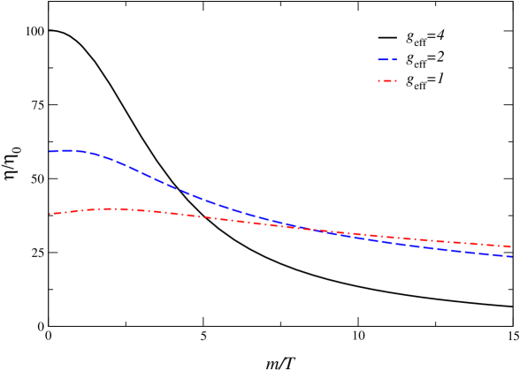
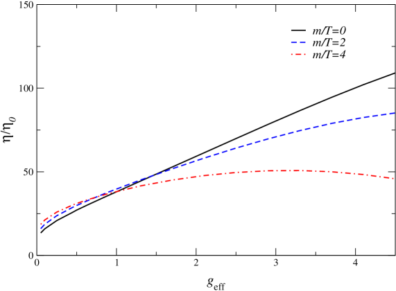
Figure 10: Shear viscosity vs. the fermion mass $m$ for various values of $g_{\rm eff}$.

Figure 11: Shear viscosity vs. the effective coupling constant $g_{\rm eff}$ for various values of the fermion mass $m$.

Figure 12: Electrical conductivity vs. the fermion mass $m$ for various values of $g_{\rm eff}$.

Figure 13: Electrical conductivity vs. the effective coupling constant $g_{\rm eff}$ for various values of the fermion mass $m$.

We notice that the general behavior of these transport coefficients is to decrease with increasing mass except for small values of the coupling constant, where a slight increase for small masses is observed. After rescaling with $\eta_{0}$ resp. $\sigma_{0}$, the remaining dependence on the effective coupling constant is quite strong, much stronger than the subleading dependence on the quartic coupling in the case of the shear viscosity in the $O(N)$ model [15]. In the limit of vanishing fermionic mass, our results agree with those obtained in Ref. [3] using kinetic theory. In the opposite limit of very large mass, we provide in Appendix B some parametric estimates of these transport coefficients in the leading logarithmic approximation, see Eq. (154), which corroborate the behavior shown in the plots. The difference between the mass dependence of the shear viscosity in the $O(N)$ model [15] and in the gauge theory is due to the different mass and momentum dependence of the (transport) cross section.

In our complete leading order calculation in the large $N_{f}$ limit, the presence of the Landau pole means that, for given fermion mass, there is an upper bound on the possible values of the coupling constant, arising from the requirement that all physical scales lie well below the Landau scale $\Lambda_{L}$. For large masses $m/T\gg 1$, the typical momentum scale is not set by the temperature, but instead by $p\sim\sqrt{mT}\gg T$. Thus, the upper bound on the coupling constant decreases when the mass is increased. This implies that going to asymptotically large mass requires a restriction to the weak coupling limit.

8 Conclusions

We have presented a diagrammatic calculation of the shear viscosity and the electrical conductivity at leading order in the large $N_{f}$ expansion of QED and QCD for massive fermions.

The 2PI effective action at next-to-leading order provides in a straightforward manner appropriate integral equations which sum all the required diagrams to obtain these transport coefficients at leading order. We proved that these equations are gauge fixing independent and consistent with the Ward identity. This explicitly shows that in a fully self-consistent calculation of these transport coefficients at leading order in the 2PI framework, potential non gauge invariant contributions would be suppressed by powers of $N_{f}$. This suggests that in self-consistent applications of the 2PI effective action in gauge theories, e.g. as in far-from-equilibrium applications, potential problems related to gauge invariance and Ward identities would be small for sufficiently large $N_{f}$.

Our results show a nontrivial dependence of the shear viscosity and electrical conductivity on the mass of the fermions and the effective gauge coupling. We found that for small values of the coupling constant they increase slightly with increasing mass. For larger values of the fermion mass, both the shear viscosity and electrical conductivity decrease. It would therefore be interesting to extend current calculations of transport coefficients to include different massive fermion flavors. We also found that after taking out the expected $1/\alpha^{2}$ dependence, a strong dependence on the gauge coupling remains. When nonperturbative results obtained from lattice QCD simulations [21] are compared with perturbative ultrarelativistic expressions, these findings should be kept in mind.

Acknowledgments. Discussions with G. Moore and L. Yaffe on the large mass dependence are gratefully acknowledged. J.M.M.R. thanks the Physics Department in Swansea for its hospitality during the completion of this work. This research was supported in part by the U. S. Department of Energy under Contract No. DE-FG02-01ER41190 and No. DE-FG02-91-ER4069 and in part by the Spanish Science Ministry (Grant FPA 2002-02037) and the University of the Basque Country (Grant UPV00172.310-14497/2002). G.A. is supported by a PPARC Advanced Fellowship.

Appendix A 2PI effective action

In this appendix we summarize some useful exact relations derived from the 2PI effective action. We consider only bilocal sources, such that the path integral is

$$Z[K,H]=e^{iW[K,H]}=\int{\cal D}\bar{\psi}{\cal D}\psi{\cal D}\phi\,e^{i\left(S[\bar{\psi},\psi,\phi]+\frac{1}{2}\phi^{i}K_{ij}\phi^{j}+H_{ba}\psi^{a}\bar{\psi}^{b}\right)}.$$ (130)

We denote Bose fields collectively with $\phi^{i}$ and fermion fields with $\psi^{a}$. Indices indicate space-time as well as internal indices, and integration and summation over repeated indices is understood, e.g.,

$$H_{ba}\psi^{a}\bar{\psi}^{b}=\int_{xy}H_{\beta\alpha}(y,x)\psi^{\alpha}(x)\bar{\psi}^{\beta}(y)=\int_{xy}{\mathrm{tr}}\,H(y,x)\psi(x)\bar{\psi}(y).$$ (131)

The 2PI effective action follows from the Legendre transform

$$\Gamma[G,S]=W[K,H]-\frac{1}{2}G^{ij}K_{ij}-H_{ba}S^{ab},$$ (132)

where

$$\frac{\delta W}{\delta K_{ij}}= \frac{1}{2}G^{ij}=\frac{1}{2}\langle T_{\cal C}\phi^{i}\phi^{j}\rangle,\;\;\;\;\;\;\;\;\;\;\;\;\frac{\delta\Gamma}{\delta G^{ij}}=-\frac{1}{2}K_{ij},$$ (133)

$$\frac{\delta W}{\delta H_{ba}}= S^{ab}=\langle T_{\cal C}\psi^{a}\bar{\psi}^{b}\rangle,\;\;\;\;\;\;\;\;\;\;\;\;\;\;\;\;\frac{\delta\Gamma}{\delta S^{ba}}=-H_{ab}.$$ (134)

The effective action is written as

$$\Gamma[G,S]=\frac{i}{2}{\mathrm{Tr}}\ln G^{-1}+\frac{i}{2}{\mathrm{Tr}}\,G_{0}^{-1}(G-G_{0})-i{\mathrm{Tr}}\ln S^{-1}-i{\mathrm{Tr}}\,S_{0}^{-1}(S-S_{0})+\Gamma_{2}[G,S],$$ (135)

where

$$iG_{0\,ij}^{-1}=\frac{\delta^{2}S}{\delta\phi^{i}\delta\phi^{j}}\Big{|}_{\phi=\psi=\bar{\psi}=0},\;\;\;\;\;\;\;\;\;\;\;\;iS_{0\,ab}^{-1}=\frac{\delta^{2}S}{\delta\psi^{a}\delta\bar{\psi}^{b}}\Big{|}_{\phi=\psi=\bar{\psi}=0}.$$ (136)

Varying this effective action once yields

$$\frac{\delta\Gamma}{\delta G^{ij}}=-\frac{i}{2}\left(G^{-1}_{ij}-G_{0\,ij}^{-1}+\Pi_{ij}\right),\;\;\;\;\;\;\;\;\;\;\;\;\frac{\delta\Gamma}{\delta S^{ba}}=i\left(S^{-1}_{ab}-S_{0\,ab}^{-1}+\Sigma_{ab}\right),$$ (137)

with

$$\Pi_{ij}=2i\frac{\delta\Gamma_{2}}{\delta G^{ij}},\;\;\;\;\;\;\;\;\;\;\;\;\Sigma_{ab}=-i\frac{\delta\Gamma_{2}}{\delta S^{ba}}.$$ (138)

Varying one more time results in the relations

$$\frac{\delta^{2}\Gamma}{\delta G^{ij}\delta G^{kl}}= \frac{i}{4}\left(G^{-1}_{ik}G^{-1}_{jl}+G^{-1}_{il}G^{-1}_{jk}-\Lambda_{ij;kl}\right),$$

$$\frac{\delta^{2}\Gamma}{\delta S^{ba}\delta S^{dc}}= i\left(-S^{-1}_{ad}S^{-1}_{cb}-\Lambda_{ab;cd}\right),$$ (139)

$$\frac{\delta^{2}\Gamma}{\delta G^{ij}\delta S^{ba}}= \frac{i}{2}\Lambda_{ij;ab},$$

where we defined

$$\Lambda_{ij;kl}=4i\frac{\delta^{2}\Gamma_{2}}{\delta G^{ij}\delta G^{kl}},\;\;\;\;\;\;\;\;\Lambda_{ij;ab}=-2i\frac{\delta^{2}\Gamma_{2}}{\delta G^{ij}\delta S^{ba}},\;\;\;\;\;\;\;\;\Lambda_{ab;cd}=i\frac{\delta^{2}\Gamma_{2}}{\delta S^{ba}\delta S^{dc}}.$$ (140)

From Eqs. (133, 134) we find

$$\frac{\delta^{2}W}{\delta K_{ij}\delta K_{kl}}= \frac{i}{4}\left(G_{c}^{ij;kl}+G^{ik}G^{jl}+G^{il}G^{jk}\right),$$

$$\frac{\delta^{2}W}{\delta H_{ba}\delta H_{dc}}= i\left(G_{c}^{ab;cd}-S^{cb}S^{ad}\right),$$ (141)

$$\frac{\delta^{2}W}{\delta K_{ij}\delta H_{ba}}= \frac{i}{2}G_{c}^{ij;ab},$$

where $G_{c}^{ij;kl}$ etc. are the usual connected 4-point functions. It is convenient to use vertex functions defined by truncating legs

$$G_{c}^{ij;kl;}= G^{ii^{\prime}}G^{jj^{\prime}}G^{kk^{\prime}}G^{ll^{\prime}}\Gamma^{(4)}_{i^{\prime}j^{\prime};k^{\prime}l^{\prime};},$$

$$G_{c}^{ij;ab}= G^{ii^{\prime}}G^{jj^{\prime}}S^{aa^{\prime}}S^{b^{\prime}b}\Gamma^{(4)}_{i^{\prime}j^{\prime};a^{\prime}b^{\prime}},$$ (142)

$$G_{c}^{ab;cd;}= S^{aa^{\prime}}S^{b^{\prime}b}S^{cc^{\prime}}S^{d^{\prime}d}\Gamma^{(4)}_{a^{\prime}b^{\prime};c^{\prime}d^{\prime}}.$$

From the following identities

$$0=\frac{\delta K_{ij}}{\delta H_{ba}},\;\;\;\;\;\;\;\;\delta_{a}^{d}\delta_{b}^{c}=\frac{\delta H_{ab}}{\delta H_{dc}},\;\;\;\;\;\;\;\;0=\frac{\delta H_{ab}}{\delta K_{ij}},\;\;\;\;\;\;\;\;\frac{1}{2}\left(\delta_{i}^{k}\delta_{j}^{l}+\delta_{i}^{l}\delta_{j}^{k}\right)=\frac{\delta K_{ij}}{\delta K_{kl}},$$ (143)

we arrive at four coupled integral equations for the 4-point vertex functions:

$$\Gamma^{(4)}_{ij;ab}= \Lambda_{ij;ab}+\frac{1}{2}\Lambda_{ij;kl}G^{kk^{\prime}}G^{ll^{\prime}}\Gamma^{(4)}_{k^{\prime}l^{\prime};ab}-\Lambda_{ij;dc}S^{cc^{\prime}}S^{d^{\prime}d}\Gamma^{(4)}_{c^{\prime}d^{\prime};ab},$$

$$\Gamma^{(4)}_{ab;cd}= \Lambda_{ab;cd}+\frac{1}{2}\Lambda_{ab;ij}G^{ii^{\prime}}G^{jj^{\prime}}\Gamma^{(4)}_{i^{\prime}j^{\prime};cd}-\Lambda_{ab;fe}S^{ee^{\prime}}S^{f^{\prime}f}\Gamma^{(4)}_{e^{\prime}f^{\prime};cd},$$

$$\Gamma^{(4)}_{ab;ij}= \Lambda_{ab;ij}+\frac{1}{2}\Lambda_{ab;kl;}G^{kk^{\prime}}G^{ll^{\prime}}\Gamma^{(4)}_{k^{\prime}l^{\prime};ij}-\Lambda_{ab;dc}S^{cc^{\prime}}S^{d^{\prime}d}\Gamma^{(4)}_{c^{\prime}d^{\prime};ij},$$

$$\Gamma^{(4)}_{ij;kl}= \Lambda_{ij;kl}+\frac{1}{2}\Lambda_{ij;mn}G^{mm^{\prime}}G^{nn^{\prime}}\Gamma^{(4)}_{m^{\prime}n^{\prime};kl}-\Lambda_{ij;dc}S^{cc^{\prime}}S^{d^{\prime}d}\Gamma^{(4)}_{c^{\prime}d^{\prime};ij}.$$ (144)

In the main text we employ these equations using the $1/N_{f}$ expansion of the 2PI effective action at NLO.

Appendix B Parametric estimates

In this appendix we discuss parametric estimates in the leading logarithmic approximation, in the zero and large fermion mass limit, using a standard kinetic theory discussion (see e.g. [22]).

It follows from the hydrodynamical definitions [23] that the shear viscosity and the electrical conductivity are related to a diffusion coefficient as

$$D=\frac{\eta}{\langle{\cal E}+{\cal P}\rangle},\;\;\;\;\;\;\;\;\;\;\;\;\;\;\;D=\frac{\sigma}{\Xi},$$ (145)

where $\cal E$ is the energy density, $\cal P$ the pressure, and $\Xi$ the charge susceptibility. For parametric estimates, this diffusion constant can be taken to be the same, since similar processes determine the transport of energy momentum and charge in the large $N_{f}$ limit, namely large angle scattering between fermions. The diffusion constant can be estimated using a random walk model [24, 25] as $D=\ell_{\rm mf}\bar{v}$, where $\bar{v}$ is the average speed and $\ell_{\rm mf}\sim 1/\bar{n}\sigma_{\rm tr}$ the mean free path, with $\bar{n}$ the mean density and $\sigma_{\rm tr}$ the transport cross section [22]

$$\sigma_{\rm tr}=\int d\Omega\left(1-\cos\theta\right)\frac{d\sigma}{d\Omega}.$$ (146)

If we keep only the most divergent term in the differential cross section,

$$\frac{d\sigma}{d\Omega}\sim\frac{\alpha^{2}}{N_{f}^{2}}\frac{1}{s}\frac{1}{\theta^{4}}\;\;\;\;\;\;\;\;(p\gg m),\;\;\;\;\;\;\;\;\;\;\;\;\frac{d\sigma}{d\Omega}\sim\frac{\alpha^{2}}{N_{f}^{2}}\frac{m^{2}}{p^{4}}\frac{1}{\theta^{4}}\;\;\;\;\;\;\;\;(p\ll m),$$ (147)

where $\alpha=e^{2}/4\pi$, and we recall that the gauge coupling $e^{2}$ is rescaled with $1/N_{f}$, the transport cross section reads

$$\sigma_{\rm tr}\sim\frac{\alpha^{2}}{N_{f}^{2}T^{2}}\int d\theta\frac{1}{\theta}=\frac{\alpha^{2}}{N_{f}^{2}T^{2}}\ln\theta_{\min}^{-1}.$$ (148)

Here we used that in the relativistic case the typical momentum $p\sim\sqrt{s}\sim T$ while in the nonrelativistic case $p\sim m\bar{v}\sim\sqrt{Tm}$. Eq. (148) holds for both $p\gg m$ and $p\ll m$. The divergence at small angles is, to leading log accuracy, cut off by Debye screening [22].

For light fermions ($T\gg m$) we use that

$$\langle{\cal E}\rangle\sim\langle{\cal P}\rangle\sim N_{f}T^{4},\;\;\;\;\;\;\;\;\;\;\bar{n}\sim N_{f}T^{3},\;\;\;\;\;\;\;\;\;\;\Xi\sim N_{f}q_{f}^{2}T^{2},\;\;\;\;\;\;\;\;\;\;\bar{v}\sim 1,$$ (149)

as well as that $\theta_{\rm min}\sim q/p\sim m_{D}/T\sim e$, where $q$ is the exchanged momentum. This leads to the well-known parametric estimates [26, 1]

$$\eta\sim N_{f}^{2}\frac{T^{3}}{\alpha^{2}\ln 1/\alpha},\;\;\;\;\;\;\;\;\;\;\;\;\;\;\;\;\;\;\;\;\;\;\;\;\;\;\;\;\sigma\sim q_{f}^{2}N_{f}^{2}\frac{T}{\alpha^{2}\ln 1/\alpha}.$$ (150)

In the case of heavy fermions ($m/T\gg 1$) in the regime where scattering can be treated classically ($\alpha^{2}m/T\gg 1$) [22], the exchanged momentum $q$ can be estimated as the product of the force $\alpha/r_{D}^{2}$ and the transit time $r_{D}/\bar{v}$ for a passage at impact parameter $r_{D}$, the typical Debye distance [22]. This yields $q\sim\alpha/(r_{D}\bar{v})$. We find therefore that $\theta_{\rm min}\sim q/p\sim\alpha/(r_{D}T)$. The inverse Debye mass $r_{D}=1/m_{D}$ is determined from $m_{D}^{2}=-\Pi^{00}(p^{0}=0,{\mathbf{p}}\to 0)$. For large $m\gg T$ we find an exponentially small Debye mass,

$$m_{D}^{2}\sim\alpha m^{2}\left(\frac{T}{m}\right)^{\frac{1}{2}}e^{-m/T}\left[1+{\cal O}\left(T/m\right)\right],$$ (151)

such that

$$\log\theta_{\rm min}^{-1}\sim\frac{m}{2T}+\frac{3}{4}\log\frac{T}{\alpha^{2}m}+{\cal O}(T/m).$$ (152)

Combining this with

$$\langle{\cal E}\rangle\sim m\bar{n},\;\;\;\;\;\;\;\;\;\;\langle{\cal P}\rangle\sim T\bar{n},\;\;\;\;\;\;\;\;\;\;\Xi\sim q_{f}^{2}\bar{n}/T,\;\;\;\;\;\;\;\;\;\;\bar{v}\sim\sqrt{T/m},$$ (153)

yields

$$\eta\sim N_{f}^{2}\frac{T^{3}}{\alpha^{2}}\left(\frac{T}{m}\right)^{\frac{1}{2}},\;\;\;\;\;\;\;\;\;\;\;\;\;\;\;\;\;\;\;\;\sigma\sim q_{f}^{2}N_{f}^{2}\frac{T}{\alpha^{2}}\left(\frac{T}{m}\right)^{\frac{3}{2}}.$$ (154)

As indicated above, these expressions are valid in the leading log approximation $\log T/\alpha m_{D}\gg 1$, the large mass limit $m/T\gg 1$, as well as the classical scattering limit $\alpha^{2}m/T\gg 1$.

References

• [1] P. Arnold, G. D. Moore and L. G. Yaffe, JHEP 0011, 001 (2000) [hep-ph/0010177]; ibid. 0305 (2003) 051 [hep-ph/0302165].
• [2] G. Policastro, D. T. Son and A. O. Starinets, Phys. Rev. Lett.  87 (2001) 081601 [hep-th/0104066].
• [3] G. D. Moore, JHEP 0105, 039 (2001) [hep-ph/0104121].
• [4] M. A. Valle Basagoiti, Phys. Rev. D 66, 045005 (2002) [hep-ph/0204334].
• [5] G. Aarts and J. M. Martínez Resco, JHEP 0211, 022 (2002) [hep-ph/0209048].
• [6] D. Boyanovsky, H. J. de Vega and S. Y. Wang, Phys. Rev. D 67, 065022 (2003) [hep-ph/0212107].
• [7] A. Buchel, J. T. Liu and A. O. Starinets, Nucl. Phys. B 707, 56 (2005) [hep-th/0406264].
• [8] H. Defu, hep-ph/0501284.
• [9] A. Peshier and W. Cassing, hep-ph/0502138.
• [10] G. D. Moore, JHEP 0210, 055 (2002) [hep-ph/0209190]; A. Ipp, G. D. Moore and A. Rebhan, JHEP 0301, 037 (2003) [hep-ph/0301057]; A. Ipp and A. Rebhan, JHEP 0306, 032 (2003) [hep-ph/0305030].
• [11] J. Berges and J. Cox, Phys. Lett. B 517, 369 (2001) [hep-ph/0006160]; B. Mihaila, F. Cooper and J. F. Dawson, Phys. Rev. D 63, 096003 (2001) [hep-ph/0006254]; G. Aarts and J. Berges, Phys. Rev. D 64, 105010 (2001) [hep-ph/0103049]; J. Berges, Nucl. Phys. A 699, 847 (2002) [hep-ph/0105311]; G. Aarts and J. Berges, Phys. Rev. Lett.  88, 041603 (2002) [hep-ph/0107129]; G. Aarts, D. Ahrensmeier, R. Baier, J. Berges and J. Serreau, Phys. Rev. D 66, 045008 (2002) [hep-ph/0201308]; F. Cooper, J. F. Dawson and B. Mihaila, Phys. Rev. D 67 (2003) 051901 [hep-ph/0207346]; ibid. 056003 [hep-ph/0209051]; hep-ph/0502040; J. Berges and J. Serreau, Phys. Rev. Lett.  91 (2003) 111601 [hep-ph/0208070]; J. Berges, S. Borsányi and J. Serreau, Nucl. Phys. B 660 (2003) 51 [hep-ph/0212404]; B. Mihaila, Phys. Rev. D 68, 036002 (2003) [hep-ph/0303157]; S. Juchem, W. Cassing and C. Greiner, Phys. Rev. D 69 (2004) 025006 [hep-ph/0307353]; Nucl. Phys. A 743, 92 (2004) [nucl-th/0401046]; J. Berges, S. Borsányi and C. Wetterich, Phys. Rev. Lett.  93, 142002 (2004) [hep-ph/0403234]; A. Arrizabalaga, J. Smit and A. Tranberg, JHEP 0410, 017 (2004) [hep-ph/0409177].
• [12] G. Aarts and J. M. Martínez Resco, Phys. Rev. D 68 (2003) 085009 [hep-ph/0303216].
• [13] A. Arrizabalaga and J. Smit, Phys. Rev. D 66, 065014 (2002) [hep-ph/0207044]; E. Mottola, in Proceedings of SEWM2002, Heidelberg, Germany, 2-5 Oct 2002 [hep-ph/0304279]; M. E. Carrington, G. Kunstatter and H. Zaraket, hep-ph/0309084; A. Peshier, Phys. Rev. D 70, 034016 (2004) [hep-ph/0403225]; J. O. Andersen and M. Strickland, Phys. Rev. D 71, 025011 (2005) [hep-ph/0406163].
• [14] G. Aarts and J. M. Martínez Resco, in Proceedings of SEWM04, Helsinki, Finland, 16-19 June 2004 [hep-ph/0409090].
• [15] G. Aarts and J. M. Martínez Resco, JHEP 0402 (2004) 061 [hep-ph/0402192].
• [16] J. M. Cornwall, R. Jackiw and E. Tomboulis, Phys. Rev. D 10 (1974) 2428; J.M. Luttinger and J.C. Ward, Phys. Rev. 118 (1960) 1417; G. Baym, Phys. Rev. 127 (1962) 1391.
• [17] H. van Hees and J. Knoll, Phys. Rev. D 65, 025010 (2002) [hep-ph/0107200]; ibid. 105005 (2002) [hep-ph/0111193]; J. P. Blaizot, E. Iancu and U. Reinosa, Phys. Lett. B 568 (2003) 160 [hep-ph/0301201]; Nucl. Phys. A 736, 149 (2004) [hep-ph/0312085]; F. Cooper, B. Mihaila and J. F. Dawson, Phys. Rev. D 70, 105008 (2004) [hep-ph/0407119]; J. Berges, S. Borsányi, U. Reinosa and J. Serreau, hep-ph/0409123.
• [18] V. V. Lebedev and A. V. Smilga, Physica A 181 (1992) 187.
• [19] J. P. Blaizot and E. Iancu, Phys. Rev. D 55, 973 (1997) [hep-ph/9607303].
• [20] G. Aarts and J. M. Martínez Resco, in Proceedings of SEWM2002, Heidelberg, Germany, 2-5 Oct 2002 [hep-ph/0212268].
• [21] S. Gupta, Phys. Lett. B 597, 57 (2004) [hep-lat/0301006]; A. Nakamura and S. Sakai, Phys. Rev. Lett.  94, 072305 (2005) [hep-lat/0406009]; G. Aarts and J. M. Martínez Resco, JHEP 0204 (2002) 053 [hep-ph/0203177]; Nucl. Phys. Proc. Suppl.  119 (2003) 505 [hep-lat/0209033].
• [22] E. M. Lifshitz and L. P. Pitaevskii, Physical Kinetics (Pergamon Press, 1981).
• [23] L. P. Kadanoff and P. C. Martin, Ann. Phys. 24, 419 (1963), reprinted as Ann. Phys. 281, 800 (2000).
• [24] D. Forster, Hydrodynamic Fluctuations, Broken Symmetry and Correlation Functions (Addison Wesley, 1989).
• [25] S. Jeon, Phys. Rev. D 52, 3591 (1995) [hep-ph/9409250].
• [26] G. Baym, H. Monien, C. J. Pethick and D. G. Ravenhall, Phys. Rev. Lett.  64 (1990) 1867.