Tachyonic Squarks in Split Supersymmetry

Abstract

The decoupling of scalar particles in split supersymmetry makes the spectrum of squarks irrelevant for low energy processes. Nevertheless, the structure of the vacuum is sensitive to the spectrum of squarks, even when the supersymmetry breaking scale is large. In this note, we show that in certain regions of the parameter space, squarks could develop radiatively tachyonic masses, thus breaking electric charge and color. We discuss the constraints that follow from the requirement of charge and color conservation, and we comment on the implications for model building.

IFT-UAM/CSIC-05-18

1 Introduction

Low energy supersymmetry stands since many years as the most attractive extension of the Standard Model. It provides not only a theoretically well motivated solution to the hierarchy problem, but also predicts the unification of the gauge couplings at a high energy scale [1] and provides a promising dark matter candidate, the neutralino [2]. Despite the great interest of the supersymmetric extension of the Standard Model, it is not free of problems. It suffers from too large contributions to flavour changing neutral currents, CP violation and proton decay. Nevertheless, it is possible to circumvent all these problems by adjusting the parameters of the model, being the most simple solution to assume that squark and slepton masses are sufficiently large, at least for the first two generations. Above all, the most important drawback for the Supersymmetric Standard Model is the failure in the quest of the Higgs boson, predicted to be fairly light in its minimal version, the MSSM. To satisfy the experimental constraints, soft masses in the Higgs sector have to be somewhat larger than the electroweak scale, introducing a milder hierarchy problem.

This milder version of the naturalness problem could be interpreted as an indication for physics beyond the Minimal Supersymmetric Standard Model. It could be alleviated, for instance, by extending the model with one extra singlet, solving at the same time the $\mu$-problem [3]. A more radical attitude to the naturalness problem was recently advocated by Arkani-Hamed and Dimopoulos [4], and consists in just accepting a fine-tuning in the breaking of the electroweak symmetry, arguing that there already exists a second (and more severe) hierarchy problem in the Supersymmetric Standard Model, namely the cosmological constant problem. With this guiding principle, there is no reason to keep the scalar particles light, as long as an (unspecified) mechanism can fine tune the Higgs vacuum expectation value to 246 GeV and the cosmological constant to $\sim(10^{-3}~{}{\rm eV})^{4}$.

The authors in [4, 5, 6] also noted that making squarks and sleptons heavy provides a solution to the problems of Supersymmetric Standard Model, but does not necessarily destroy the successes. Keeping the gauginos and higgsinos at the electroweak scale, gauge unification is preserved and the neutralino is still a viable candidate for the dark matter of the Universe. Following Giudice and Romanino, we will call this scenario split supersymmetry: a scenario with light fermion masses and heavy scalar masses, except for the Standard Model Higgs, fine tuned to yield a correct $Z$ boson mass and a small cosmological constant. Recently, some of the low energy implications of this scenario have been discussed, such as electric dipole moments [6, 7], collider signatures [5, 8], Higgs physics and the electroweak symmetry breaking [5, 9, 10], dark matter [5, 6, 11] or cosmic ray showers [12].

The decoupling of the scalar particles might suggest that the spectrum of squarks and sleptons is completely irrelevant for the low-energy phenomenology. In this note, we would like to point out that the structure of the supersymmetric vacuum is indeed sensitive to the spectrum of squarks and sleptons, even when the scale of supersymmetry breaking is large. We will show that under certain conditions, radiative corrections could induce tachyonic stop masses, thus leading to charge and colour breaking. The reason for this can be easily understood from the well known mechanism of radiative electroweak symmetry breaking in the MSSM [13]. Radiative corrections from the top Yukawa coupling can drive the up-type Higgs mass squared to negative values, thus breaking $SU(2)_{L}\times U(1)_{Y}$. This is not normally the case for the stop mass squared, since the gluino radiative corrections induce a positive contribution to the mass squared that is usually large enough to keep the stop mass squared positive. In split supersymmetry the gluino mass is much smaller than the scalar masses, so this positive contribution is no longer important, and in consequence there exists the possibility of generating radiatively tachyonic stop masses. In this note we will discuss the constraints that this imposes on the scenario of split supersymmetry.

2 Running of the squark masses

Let us consider first scenarios with low $\tan\beta$, so that only the top Yukawa coupling is relevant. Later on, we will discuss scenarios with large $\tan\beta$ for which the effects from the bottom and tau Yukawa couplings also have to be taken into account. The one loop renormalization group equations for the left and right handed stops and the up-type Higgs doublet read:

$$\frac{dm_{\widetilde{t}_{L}}^{2}}{dt}=\frac{1}{16\pi^{2}}\left[\frac{16}{3}g^{2}_{3}M^{2}_{3}+3g^{2}_{2}M^{2}_{2}+\frac{1}{15}g^{2}_{1}M^{2}_{1}-h_{t}^{2}(m_{\widetilde{t}_{L}}^{2}+m_{\widetilde{t}_{R}}^{2}+m_{H_{u}}^{2}+A_{t}^{2})\right],$$

$$\frac{dm_{\widetilde{t}_{R}}^{2}}{dt}=\frac{1}{16\pi^{2}}\left[\frac{16}{3}g^{2}_{3}M^{2}_{3}+\frac{16}{15}g^{2}_{1}M^{2}_{1}-2h_{t}^{2}(m_{\widetilde{t}_{L}}^{2}+m_{\widetilde{t}_{R}}^{2}+m_{H_{u}}^{2}+A_{t}^{2})\right],$$

$$\frac{dm_{H_{u}}^{2}}{dt}=\frac{1}{16\pi^{2}}\left[3g^{2}_{2}M^{2}_{2}+\frac{3}{5}g^{2}_{1}M^{2}_{1}-3h_{t}^{2}(m_{\widetilde{t}_{L}}^{2}+m_{\widetilde{t}_{R}}^{2}+m_{H_{u}}^{2}+A_{t}^{2})\right],$$ (1)

where $t=\log(M_{X}^{2}/Q^{2})$, $Q$ is the renormalization scale and $M_{X}$ is the scale at which the soft terms are generated, that we use as boundary condition to run the renormalization group equations. Inspired by the gravity mediated supersymmetry breaking framework, we will assume that the soft breaking terms are generated at the reduced Planck scale, $M_{P}=M_{Planck}/\sqrt{8\pi}=2.4\times 10^{18}$ GeV.

The set of differential equations (1) can be solved analytically [14, 15]. In the limit of split supersymmetry, gaugino masses are much smaller than the scalar masses, and the trilinear soft terms, being protected by the same R-symmetry that protects gaugino masses, are also expected to be much smaller than the scalar masses. Therefore, the analytical expression for the solution greatly simplifies, and reads:

$$m_{\widetilde{t}_{L}}^{2}(t)=m_{\widetilde{t}_{L}}^{2}(0)-\frac{h_{t}^{2}(0)}{(4\pi)^{2}}\frac{F(t)}{D(t)}[m_{H_{u}}^{2}(0)+m_{\widetilde{t}_{R}}^{2}(0)+m_{\widetilde{t}_{L}}^{2}(0)],$$

$$m_{\widetilde{t}_{R}}^{2}(t)=m_{\widetilde{t}_{R}}^{2}(0)-2\frac{h_{t}^{2}(0)}{(4\pi)^{2}}\frac{F(t)}{D(t)}[m_{H_{u}}^{2}(0)+m_{\widetilde{t}_{R}}^{2}(0)+m_{\widetilde{t}_{L}}^{2}(0)],$$

$$m_{H_{u}}^{2}(t)=m_{H_{u}}^{2}(0)-3\frac{h_{t}^{2}(0)}{(4\pi)^{2}}\frac{F(t)}{D(t)}[m_{H_{u}}^{2}(0)+m_{\widetilde{t}_{R}}^{2}(0)+m_{\widetilde{t}_{L}}^{2}(0)],$$ (2)

where

$$F(t) \equiv \int_{0}^{t}E(t^{\prime})dt^{\prime},$$ (3)

$$D(t) \equiv 1+6\frac{h_{t}^{2}(0)}{16\pi^{2}}F(t)$$ (4)

and

$$E(t) \equiv (1+\frac{g^{2}_{3}(0)}{16\pi^{2}}b_{3}t)^{(16/{3b_{3}})}~{}(1+\frac{g^{2}_{2}(0)}{16\pi^{2}}b_{2}t)^{(3/{b_{2}})}~{}(1+\frac{g^{2}_{1}(0)}{16\pi^{2}}b_{1}t)^{(13/{15b_{1}})},$$ (5)

being $(b_{1},b_{2},b_{3})\equiv(33/5,1,-3)$ the coefficients of the beta functions for the gauge couplings.

If the left-handed or the right-handed stop mass squared are driven to negative values before they decouple, the corresponding field will acquire a vacuum expectation value, thus yielding a vacuum where charge and colour are not conserved. This situation is clearly undesirable and to prevent it one has to require $m^{2}_{\widetilde{t}_{L}}(t_{\widetilde{m}})>0$ and $m^{2}_{\widetilde{t}_{R}}(t_{\widetilde{m}})>0$, where $t_{\widetilde{m}}=\log(M^{2}_{X}/{\widetilde{m}}^{2})$ and $\widetilde{m}$ is the typical size of the soft terms. These conditions translate into constraints on the scalar mass spectrum, that otherwise is completely unconstrained by low energy experiments.

For definiteness, let us discuss first the limit in which the top Yukawa coupling is barely perturbative at the cut-off scale, i.e. the infrared fixed point scenario, recently revisited for the framework of split supersymmetry in [16]. In this limit, squark masses quickly reach the fixed point (as long as $\widetilde{m}\mathrel{\raise 1.29167pt\hbox{$<$\kern-7.5pt\lower 4.30554pt\hbox{$\sim$}}}10^{16}$ GeV), usually before the squarks decouple. The corresponding masses can be read from eqs.(2) by taking the limit $h_{t}(0)\rightarrow\infty$, or by substituting

$$\frac{h_{t}^{2}(0)}{(4\pi)^{2}}\frac{F(t)}{D(t)}\simeq\frac{1}{6}.$$ (6)

The result is

$$m^{2}_{\widetilde{t}_{L}}(t_{\widetilde{m}})\simeq\frac{1}{6}[5\,m_{\widetilde{t}_{L}}^{2}(0)-m_{H_{u}}^{2}(0)-m_{\widetilde{t}_{R}}^{2}(0)],$$

$$m^{2}_{\widetilde{t}_{R}}(t_{\widetilde{m}})\simeq\frac{1}{3}[2\,m_{\widetilde{t}_{R}}^{2}(0)-m_{H_{u}}^{2}(0)-m_{\widetilde{t}_{L}}^{2}(0)],$$

$$m^{2}_{H_{u}}(t_{\widetilde{m}})\simeq\frac{1}{2}[m_{H_{u}}^{2}(0)-m_{\widetilde{t}_{L}}^{2}(0)-m_{\widetilde{t}_{R}}^{2}(0)].$$ (7)

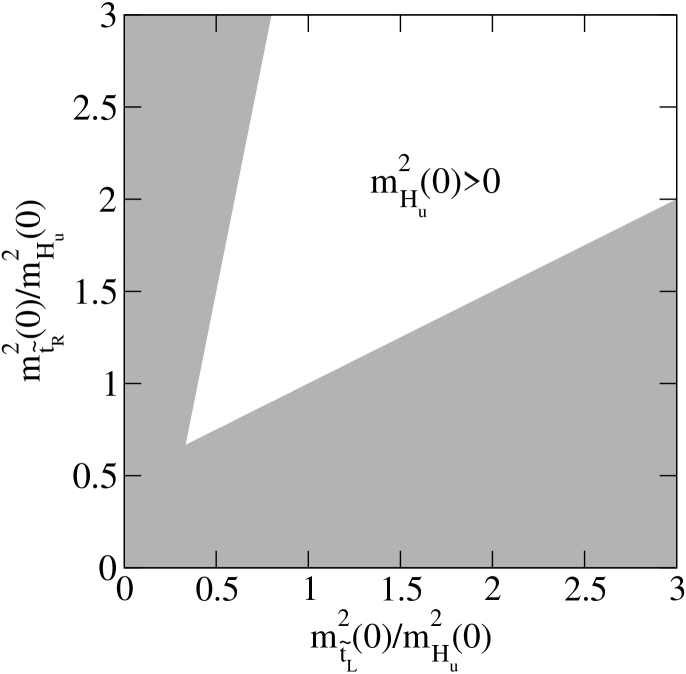
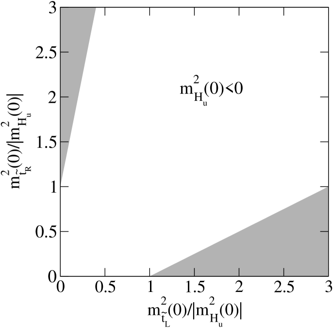
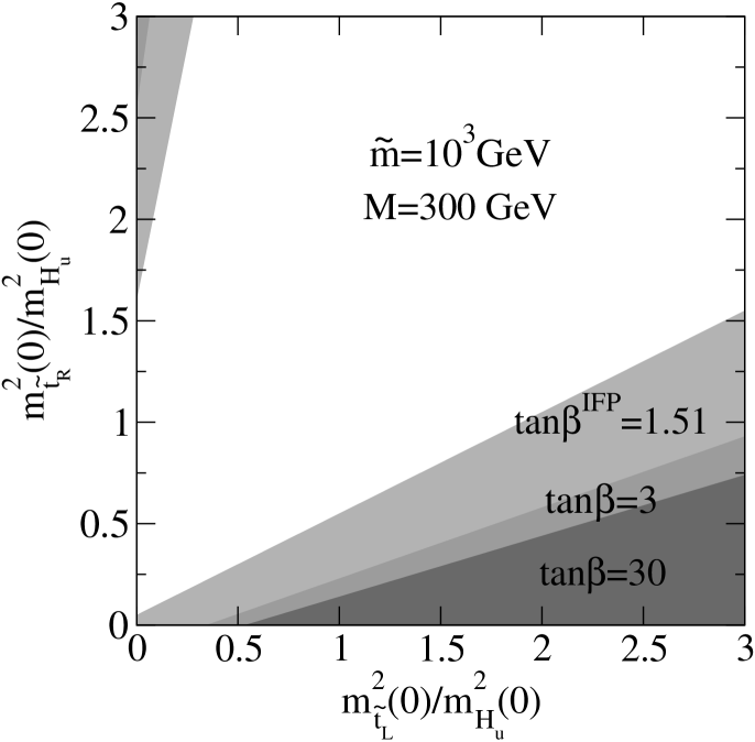
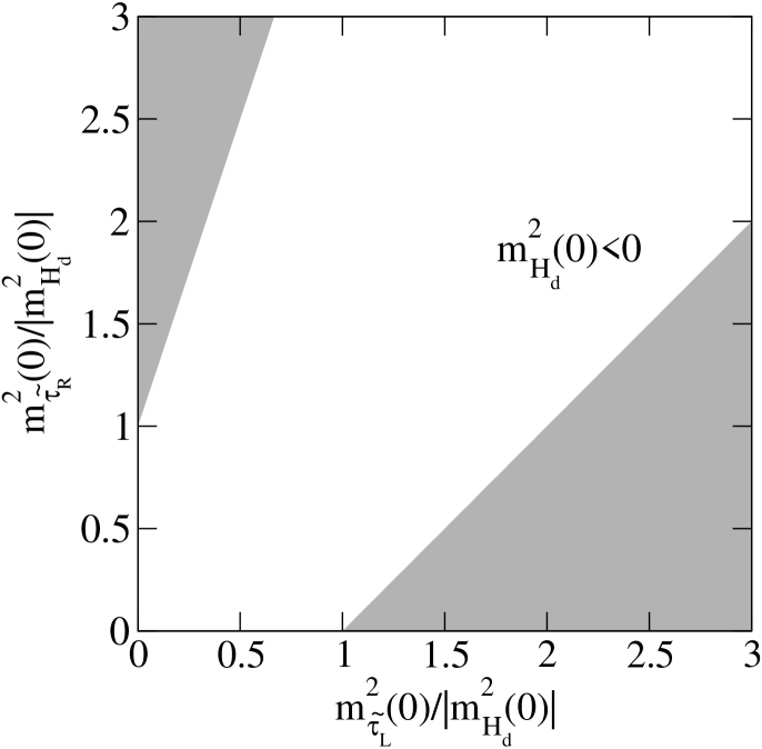
The region of the parameter space allowed from the requirement of charge and colour conservation is shown in Fig 1. The parameter space is span by the left and right handed stop masses squared relative to the up-type Higgs mass squared, whose absolute value we assume equal to $\widetilde{m}^{2}$. In the left plot we have assumed that the up-type Higgs mass squared is positive at the reduced Planck scale, so that the electroweak symmetry breaking is triggered by the familiar mechanism of dimensional transmutation. For this to happen, the soft masses at the high energy scale should satisfy the constraint $m_{H_{u}}^{2}(0)-m_{\widetilde{t}_{L}}^{2}(0)-m_{\widetilde{t}_{R}}^{2}(0)<0$. Notice that the requirement of positive stop masses squared is sufficient to guarantee the radiative breaking of the electroweak symmetry. In this case, we find that large areas in the region with $m^{2}_{H_{u}}\mathrel{\raise 1.29167pt\hbox{$>$\kern-7.5pt\lower 4.30554pt\hbox{$\sim$}}}m^{2}_{\widetilde{t}_{L},\widetilde{t}_{R}}$ are in conflict with the requirement of charge and colour conservation. On the other hand, if there is a mechanism that will eventually fine-tune the $Z$ mass to a small value, one cannot exclude the possibility that the electroweak symmetry breaking is taking place already at $M_{P}$. It could happen that the breaking of supersymmetry gives rise to tachyonic up-type Higgs masses, thus leading to the breaking of the electroweak symmetry at tree level. In the case that the Higgs mass is already tachyonic to start with, the conditions $m^{2}_{\widetilde{t}_{L}}(t_{\widetilde{m}})>0$ and $m^{2}_{\widetilde{t}_{R}}(t_{\widetilde{m}})>0$ would be easier to fulfill, as can be realized from Fig.1, right plot.

   

Figure 1: Allowed region in the stop parameter space from imposing the requirement of charge and colour conservation, in the infrared fixed point limit for the top Yukawa coupling. In the left plot, it is shown the case in which the up-type Higgs mass squared is positive at the cut-off scale, whereas in the right plot we assume that it is negative.

In a scenario with strict universality at the high energy scale, stops will not develop tachyonic masses. Nevertheless, the large mass splitting between the left-handed and the right-handed stops, that belong to the same 10-plet of $SU(5)$, would spoil the successful prediction for gauge unification.

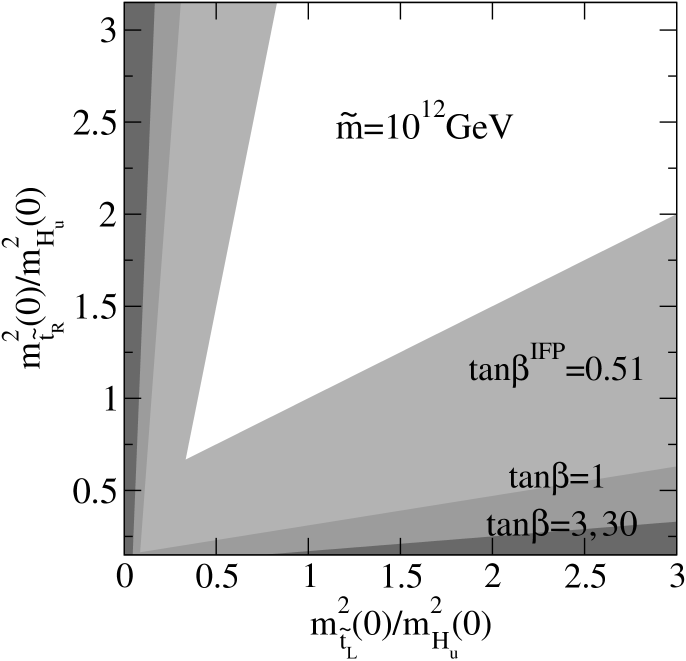
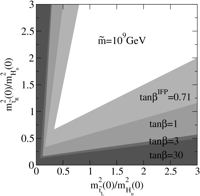
As $\tan\beta$ increases and one gets away from the top infrared fixed point, the top Yukawa coupling becomes smaller and the evolution of the squark masses squared towards negative values slows down. Therefore, the constraints on the squark parameter space that follow from the condition of charge and colour conservation relax. This is illustrated in Fig.2 for different values of $\tan\beta$ and the soft supersymmetry breaking scale, $\widetilde{m}$. Notice that for a fixed $\tan\beta$ the constraints are more restrictive as $\widetilde{m}$ becomes smaller. The reason is that the squark masses are running towards negative vales for longer, so it is easier to develop tachyonic masses. This behaviour holds as long as the gaugino masses are much smaller than $\widetilde{m}$. For values of $\widetilde{m}$ close to the electroweak scale, i.e. the standard low energy supersymmetry breaking scenario, gaugino masses (particularly the gluino mass) can be large enough to stop the running of the squark masses squared towards negative values. One can estimate the size of the gaugino masses and $\widetilde{m}$ at which this happens from the full solution to eq.(1). Assuming for simplicity that the trilinear soft terms vanish at $M_{P}$, one obtains:

$$m^{2}_{\widetilde{t}_{L}}(t) = m^{2}_{\widetilde{t}_{L}}(0)+M^{2}\left(\frac{1}{3}e(t)+\frac{8}{3}\frac{\alpha_{3}(0)}{4\pi}f_{3}(t)+\frac{\alpha_{2}(0)}{4\pi}f_{2}(t)-\frac{1}{9}\frac{\alpha_{1}(0)}{4\pi}f_{1}(t)\right)$$

$$-\frac{h_{t}^{2}(0)}{(4\pi)^{2}}\frac{F(t)}{D(t)}(m_{H_{u}}^{2}(0)+m_{\widetilde{t}_{R}}^{2}(0)+m_{\widetilde{t}_{L}}^{2}(0)),$$

$$m^{2}_{\widetilde{t}_{R}}(t) = m^{2}_{\widetilde{t}_{R}}(0)+M^{2}\left(\frac{2}{3}e(t)-H_{8}(t)\right)-2\frac{h_{t}^{2}(0)}{(4\pi)^{2}}\frac{F(t)}{D(t)}(m_{H_{u}}^{2}(0)+m_{\widetilde{t}_{R}}^{2}(0)+m_{\widetilde{t}_{L}}^{2}(0)),$$ (8)

where $e,f_{1,2,3}$ and $H_{8}$ are known functions, independent of $\tan\beta$, that can be found in the Appendix B of ref.[14]. For $\widetilde{m}=10^{3}$GeV, the result can be approximated by

$$m_{\widetilde{t}_{L}}^{2}(t)\simeq m_{\widetilde{t}_{L}}^{2}(0)-\frac{1.7h_{t}^{2}(0)}{1+10.4h_{t}^{2}(0)}(m_{H_{u}}^{2}(0)+m_{\widetilde{t}_{R}}^{2}(0)+m_{\widetilde{t}_{L}}^{2}(0))+4.7M^{2},$$

$$m_{\widetilde{t}_{R}}^{2}(t)\simeq m_{\widetilde{t}_{R}}^{2}(0)-\frac{3.5h_{t}^{2}(0)}{1+10.4h_{t}^{2}(0)}(m_{H_{u}}^{2}(0)+m_{\widetilde{t}_{R}}^{2}(0)+m_{\widetilde{t}_{L}}^{2}(0))+3.5M^{2}.$$ (9)

In Fig.2, lower right plot we show the allowed parameter space for the case with universal gaugino masses of $M=300$ GeV. One finds that a larger region is now allowed, even for the infrared fixed point scenario. For $\widetilde{m}=M$, the whole parameter space in the plots, $0\leq m_{\widetilde{t}_{L},t_{R}}^{2}(0)\leq 3m_{H_{u}}^{2}(0)$, becomes allowed for any value of $\tan\beta$.

   

   

Figure 2: Allowed regions in the stop parameter space from imposing the requirement of charge and colour conservation for different values of $\tan\beta$ and the supersymmetry breaking mass scale, $\widetilde{m}$. The lower right plot corresponds to a situation approaching the conventional MSSM scenario, where the gaugino masses, $M$, start to be relevant for the analysis.

Therefore, from the point of view of charge and colour breaking, scenarios of split supersymmetry with intermediate values for the soft masses ($\sim 10^{6}-10^{9}$ GeV) are disfavoured with respect to the conventional MSSM scenario with electroweak soft masses ($\sim 10^{3}$ GeV), where the gluinos protect the stop masses from becoming tachyonic. Scenarios with very large soft masses ($\sim 10^{12}$ GeV) are also favoured, since the squark masses are running over a smaller energy range, and the renormalization effects are normally not large enough to generate tachyonic masses. This value is close to the upper bound on the supersymmetry breaking scale in split supersymmetry of ${\cal O}(10^{13}$GeV) for a 1 TeV gluino, coming from negative searches of abnormally heavy isotopes [4]. On the other hand, when the up-type Higgs mass squared is already negative at $M_{P}$, large regions of the parameter space also become allowed.

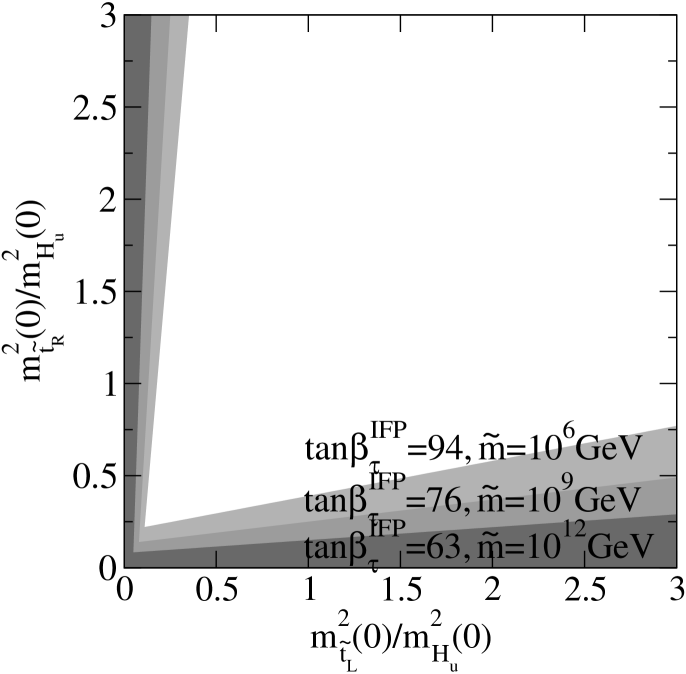
Let us comment now on the situation in which $\tan\beta$ is large. Whereas the top Yukawa coupling does not change substantially as $\tan\beta$ increases, the bottom and tau Yukawa coupling indeed do, and their effects have to be taken into account. The allowed range for $\tan\beta$ is limited from above by the appearance of a Landau pole for the tau Yukawa coupling, which occurs at $\tan\beta\simeq 94$, 76 and 63 for $\widetilde{m}=10^{12}$, $10^{9}$ and $10^{6}$ GeV, respectively. In this range, the bottom Yukawa coupling always remains perturbative until $M_{P}$, being the corresponding values at the cut-off scale $h_{b}(0)\simeq 2.8$, 3.4 and 6.9 respectively (notice that in split supersymmetry the prediction for bottom-tau unification is lost). In this regime, left-handed stop masses squared are driven to negative values faster than for intermediate values of $\tan\beta$, while the running of the right-handed stops is not modified substantially. The effect of the bottom Yukawa coupling on the left-handed stop mass is not very important numerically, and the allowed region in the stop parameter space is similar to the case with intermediate values of $\tan\beta$, as can be realized from Fig.3, left plot, where we show the allowed region in the stop parameter space for different values of the soft SUSY breaking scale, $\widetilde{m}$, and for the value of $\tan\beta$ that corresponds to the infrared fixed point limit for the tau Yukawa coupling, $\tan\beta_{\tau}^{{\rm IFP}}$.

   

Figure 3: Allowed region in the stop (left plot) and sbottom (right plot) parameter spaces from imposing the requirement of charge and colour conservation, in the infrared fixed point limit for the tau Yukawa coupling and for different values of the SUSY breaking mass scale, $\widetilde{m}$.

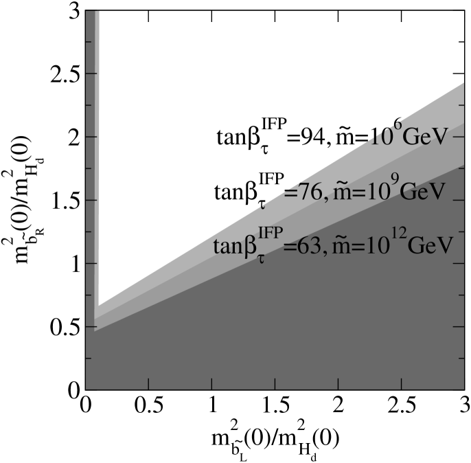
The large bottom and tau Yukawa couplings could drive the sbottom and stau masses squared negative, giving rise to constraints on the sbottom and stau parameter spaces. Despite the bottom Yukawa coupling never reaches the Landau pole, it can be large enough to induce radiatively tachyonic masses for the sbottoms, particularly for the values of $\tan\beta$ corresponding to the infrared fixed point limit for the tau Yukawa coupling. This is illustrated in Fig.3, right plot, where we show the allowed region in the sbottom parameter space in this limit. On the other hand, since the tau Yukawa coupling can become very large, the constraints for the stau parameter space can be stronger. In the infrared fixed point limit for the tau Yukawa coupling, the constraints read

$$m_{\widetilde{e}}^{2}(0)-m^{2}_{H_{d}}(0)-m^{2}_{\widetilde{L}}(0)>0,$$

$$3m_{\widetilde{L}}^{2}(0)-m^{2}_{H_{d}}(0)-m^{2}_{\widetilde{e}}(0)>0.$$ (10)

   

Figure 4: Allowed region in the stau parameter space from imposing the requirement of charge conservation, in the infrared fixed point limit for the tau Yukawa coupling. In the left plot, it is shown the case in which the down-type Higgs mass squared is positive at the cut-off scale, whereas in the right plot we assume that it is negative.

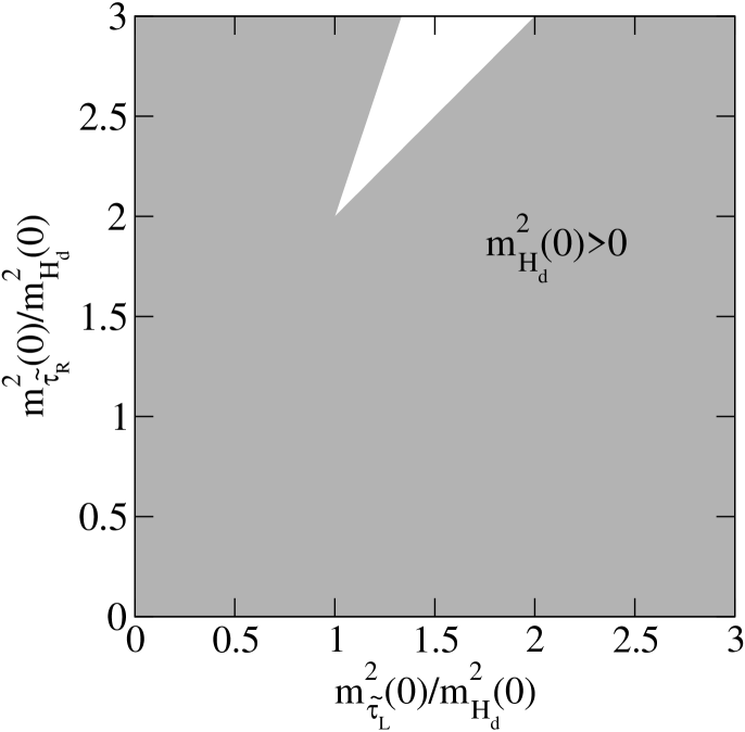
As can be realized from fig.4, the constraints on the parameter space from requiring positive stau masses squared at the decoupling scale are very strong. However, these constraints relax as $\tan\beta$ decreases and practically disappear for small values of $\tan\beta$. If the particle content of the MSSM is extended with right-handed neutrinos in order to give masses to neutrinos, then the right-handed neutrino Yukawa couplings would also contribute to the running of the stau at energies larger than the decoupling scale of the right-handed neutrinos. If the neutrino Yukawa couplings are of order one, the running of the stau mass squared towards negative values would be considerably accelerated, and this would translate into stronger bounds on the parameter space, particularly for small values of $\tan\beta$, for which the tau Yukawa coupling is small.

3 Discussion

We have shown that a split spectrum in supersymmetric theories is not enough to guarantee the phenomenological viability of a particular model. Although the decoupling of squarks and sleptons guarantees the suppression of flavour changing neutral currents, CP violating effects and proton decay, it does not guarantee that the vacuum is going to conserve electric charge and colour. When the scalar mass spectrum is non-universal, stops could acquire radiatively tachyonic masses, which is clearly an undesirable feature. It is important to stress that despite universality of the scalar masses is a common assumption in analyses of the supersymmetry parameter space, this situation is rather exceptional when constructing supersymmetric models. Most explicit scenarios of supersymmetry breaking predict non-universal scalar masses, where the analysis presented in this note is particularly relevant.

Models with split supersymmetry probably require D-term supersymmetry breaking. Although it is possible to obtain a split spectrum breaking supersymmetry giving a vacuum expectation value to an F-term, this also breaks spontaneously the R-symmetry, usually generating gaugino masses and trilinear terms of the same order of the scalar masses. In contrast, D-term supersymmetry breaking does not lead to R-symmetry breaking. This renders vanishing gaugino masses and trilinear soft terms at lowest order, which constitutes an essential feature of split supersymmetry (to generate them it is necessary to add non-renormalizable operators in the Kähler potential). If supersymmetry is indeed broken by the vacuum expectation value of a D-term, the soft scalar masses are determined by the charges of the particles under a particular gauge group, normally generating a non-universal spectrum. Needless to say, the charges have to be arranged in such a way that tachyonic masses are not arising already at tree level (with the exception of the higgses, possibility that would lead to the breaking of the electroweak symmetry already at a high-energy scale).

Some models with split supersymmetry have been constructed along this lines. The model of Babu, Enkhbat and Mukhopadhyaya [17] utilizes an anomalous $U(1)$ symmetry and a gaugino condensate to trigger supersymmetry breaking. The anomalous $U(1)$ symmetry is horizontal, thus providing also an explanation for the quark and lepton masses and mixing angles. In this model, the different charges of the particles under the anomalous $U(1)$ generates a scalar mass spectrum that is non-universal. There are however some massless fields in the limit of global supersymmetry, namely the two Higgs doublets and the third generation of the 10-plet of $SU(5)$ (they have to be neutral under the anomalous $U(1)$ in order to reproduce the observed masses and mixing angles). These particles acquire masses of the order of the gravitino mass through supergravity corrections, and could also be non-universal if the Kähler potential is non-minimal.

A different class of models was proposed by Antoniadis and Dimopoulos [19], and is based on type I string theory with internally magnetized D9 branes . In the T-dual picture, the model can be described by intersecting branes, with broken supersymmetry when the branes are intersecting at arbitrary angles. In the four dimensional effective theory, the breaking of supersymmetry can be interpreted as a D-term supersymmetry breaking. Therefore, the different scalar fields will acquire masses that depend on the D-terms associated to the different $U(1)$s of the theory (or in the dual picture, on the magnetic fields in the compact dimensions). In general, the D-terms are different for each $U(1)$, leading to a non-universal spectrum.

Finally, we would like to mention that in scenarios with split supersymmetry there exists a second threat for charge and colour conservation, namely the appearance of unbounded from below directions in the effective potential, that could lead to deep charge and colour breaking minima after including radiative corrections [21]. Again, whether these directions appear or not depends on the spectrum on squarks and sleptons, but not on the scale of supersymmetry breaking, therefore they could also arise in models with split supersymmetry. Nevertheless, it has been argued in [22] that even if they appear, the decay rate of the metastable electroweak minimum into the global minimum is very suppressed, so that the lifetime of the metastable minimum is usually longer than the age of the Universe. In consequence, the constraints that would follow from requiring the absence of unbounded from below directions could be avoided if one accepts that our electroweak vacuum is a metastable minimum with a small cosmological constant. This hypothesis might look dubious, however, in the spirit of split supersymmetry, it could be justified by some anthropic principle. Hence, the only constraints on the scalar spectrum that are robust are the ones discussed in this note, namely the possibility of radiative generation of tachyonic squark masses.

4 Conclusions

Split supersymmetry is a daring proposal to solve all the problems of the Supersymmetric Standard Model, while preserving the successes. The decoupling of the scalar particles, except for the Standard Model Higgs, suppresses flavour changing neutral currents, electric dipole moments and the rates for proton decay. Besides, imposing global symmetries to keep the gauginos and higgsinos light, preserves the nice features of gauge unification and the neutralino as a dark matter candidate.

If this scenario is realized in nature, squarks and sleptons would not have any observable effect in low energy processes, neither at tree level nor at the radiative level. However, we have remarked in this note that their spectrum is not totally unconstrained, even though squarks and sleptons are completely decoupled at low energies, and we have discussed the implications for building models with split supersymmetry. We have shown that the structure of the vacuum depends crucially on the spectrum of squarks and sleptons, and we have derived the constraints that follow from the requirement of charge and colour conservation. To be precise, certain patterns of supersymmetry breaking could induce radiatively tachyonic masses for the stops (and for the staus when $\tan\beta$ is large), thus breaking electric charge and colour. In particular, models with an intermediate supersymmetry breaking scale ($\widetilde{m}\sim 10^{6}-10^{9}$ GeV) are disfavoured with respect to the conventional MSSM scenario with low energy supersymmetry breaking ($\widetilde{m}\sim 10^{3}$ GeV). We have also stressed that models with split supersymmetry probably require D-term supersymmetry breaking, leading in general to a non-universal spectrum where the constraints presented in this note are potentially dangerous.

References

- [1] S. Dimopoulos, S. Raby and F. Wilczek, Phys. Rev. D 24 (1981) 1681.
- [2] H. Goldberg, Phys. Rev. Lett. 50 (1983) 1419; L. M. Krauss, Nucl. Phys. B 227 (1983) 556; J. R. Ellis, J. S. Hagelin, D. V. Nanopoulos, K. A. Olive and M. Srednicki, Nucl. Phys. B 238 (1984) 453.
- [3] M. Bastero-Gil, C. Hugonie, S. F. King, D. P. Roy and S. Vempati, Phys. Lett. B 489 (2000) 359 [arXiv:hep-ph/0006198].
- [4] N. Arkani-Hamed and S. Dimopoulos, arXiv:hep-th/0405159.
- [5] G. F. Giudice and A. Romanino, Nucl. Phys. B 699 (2004) 65 [Erratum-ibid. B 706 (2005) 65] [arXiv:hep-ph/0406088].
- [6] N. Arkani-Hamed, S. Dimopoulos, G. F. Giudice and A. Romanino, Nucl. Phys. B 709 (2005) 3 [arXiv:hep-ph/0409232].
- [7] D. Chang, W. F. Chang and W. Y. Keung, arXiv:hep-ph/0503055; N. G. Deshpande and J. Jiang, arXiv:hep-ph/0503116.
- [8] S. h. Zhu, Phys. Lett. B 604 (2004) 207 [arXiv:hep-ph/0407072]; J. L. Hewett, B. Lillie, M. Masip and T. G. Rizzo, JHEP 0409 (2004) 070 [arXiv:hep-ph/0408248]; K. Cheung and W. Y. Keung, Phys. Rev. D 71 (2005) 015015 [arXiv:hep-ph/0408335].
- [9] M. Binger, arXiv:hep-ph/0408240; M. A. Diaz and P. F. Perez, arXiv:hep-ph/0412066; G. Gao, R. J. Oakes and J. M. Yang, arXiv:hep-ph/0412356.
- [10] S. P. Martin, K. Tobe and J. D. Wells, arXiv:hep-ph/0412424; M. Drees, arXiv:hep-ph/0501106; G. Marandella, C. Schappacher and A. Strumia, arXiv:hep-ph/0502095; N. Haba and N. Okada, arXiv:hep-ph/0502213.
- [11] A. Pierce, Phys. Rev. D 70 (2004) 075006 [arXiv:hep-ph/0406144]; A. Arvanitaki and P. W. Graham, arXiv:hep-ph/0411376; A. Masiero, S. Profumo and P. Ullio, arXiv:hep-ph/0412058; K. Cheung and C. W. Chiang, arXiv:hep-ph/0501265.
- [12] L. Anchordoqui, H. Goldberg and C. Nunez, Phys. Rev. D 71 (2005) 065014 [arXiv:hep-ph/0408284].
- [13] L. E. Ibanez and G. G. Ross, Phys. Lett. B 110 (1982) 215; J. R. Ellis, J. S. Hagelin, D. V. Nanopoulos and K. Tamvakis, Phys. Lett. B 125 (1983) 275.
- [14] L. E. Ibanez, C. Lopez and C. Munoz, Nucl. Phys. B 256 (1985) 218.
- [15] A. Lleyda and C. Munoz, Phys. Lett. B 317 (1993) 82 [arXiv:hep-ph/9308208].
- [16] K. Huitu, J. Laamanen, P. Roy and S. Roy, arXiv:hep-ph/0502052.
- [17] K. S. Babu, T. Enkhbat and B. Mukhopadhyaya, arXiv:hep-ph/0501079.
- [18] B. Kors and P. Nath, arXiv:hep-th/0411201.
- [19] I. Antoniadis and S. Dimopoulos, arXiv:hep-th/0411032.
- [20] C. Kokorelis, arXiv:hep-th/0406258.
- [21] For a clasification of all the potentially dangerous directions in the effective potential, see J. A. Casas, A. Lleyda and C. Munoz, Nucl. Phys. B 471 (1996) 3 [arXiv:hep-ph/9507294].
- [22] S. A. Abel and C. A. Savoy, Nucl. Phys. B 532, 3 (1998) [arXiv:hep-ph/9803218].