[

Weak corrections and high $E_{T}$ jets at Tevatron

Abstract

We calculate one-loop (purely) Weak (W) corrections of ${\cal O}(\alpha_{\mathrm{S}}^{2}\alpha_{\mathrm{W}})$ to the partonic cross section of two jets at Tevatron and prove that they can be larger than the tree-level ${\cal O}(\alpha_{\mathrm{S}}\alpha_{\mathrm{EW}})$ and ${\cal O}(\alpha_{\mathrm{EW}}^{2})$ Electro-Weak (EW) ones. At high transverse energy of the jets, all such corrections may lead to detectable effects of, e.g., $-10\%$ or so, with respect to the leading-order (LO) QCD term of ${\cal O}(\alpha_{\mathrm{S}}^{2})$, for the highest value so far probed by Run 2, depending on the factorisation/renormalisation scale. Besides, they increase significantly with jet transverse energy. Hence, our results show that EW corrections may be needed to fit the Standard Model (SM) to present and future Tevatron jet data.

]

As the overall energy of hard scattering processes increases one should expect a relatively large impact of perturbative EW corrections, as compared to the QCD ones. This can easily be understood (see [1] –[2] and references therein for reviews) in terms of the so-called Sudakov (leading) logarithms of the form $\alpha_{\mathrm{W}}\log^{2}({\hat{s}}/M_{W}^{2})$ (hereafter, $\alpha_{\rm{W}}\equiv\alpha_{\rm{EM}}/\sin^{2}\theta_{\rm W}$, with $\alpha_{\rm{EM}}$ the Electro-Magnetic (EM) coupling constant and $\theta_{\rm W}$ the weak mixing angle, whereas $\sqrt{\hat{s}}$ is the parton-level centre-of-mass energy), which appear in the presence of higher order weak corrections when the initial state carries a definite non-Abelian flavour and which, unlike QCD, do not cancel between virtual and real emission of $W$ bosons [3].

Furthermore, one should recall that real weak bosons are unstable and decay into high transverse momentum leptons and/or jets, which are normally captured by the detectors. In the definition of a hadronic cross section, one may then remove events with such additional particles. Hence, for typical experimental resolutions, softly and collinearly emitted weak bosons need not be included in the definition of the production cross section and one can restrict oneself to the calculation of weak effects originating from virtual corrections only. In fact, leading (and all subleading) virtual weak corrections are finite (unlike QCD, where infrared divergences mean that virtual corrections must be considered in conjunction with gluon bremsstrahlung), as the mass of the weak gauge boson provides a physical cut-off for the otherwise divergent infrared behaviour. Under these circumstances, the (virtual) exchange of $Z$ bosons also generates double logarithmic corrections, $\alpha_{\mathrm{W}}\log^{2}({\hat{s}}/M_{Z}^{2})$. Moreover, in some simpler cases, the genuinely weak contributions can be isolated in a gauge-invariant manner from purely EM effects and the latter may or may not be included in the calculation, depending on the observable being studied.

The leading, double-logarithmic, angular-independent weak logarithmic corrections are universal, i.e., they depend only on the identities of the external particles. In some instances, however, large cancellations between angular-independent and angular-dependent corrections [4] (see also [5] for two-loop results) and between leading and subleading terms [6] have been found at TeV energies. Moreover, some other considerations are in order in the specific hadronic context. Firstly, one should recall that hadron-hadron scattering events involve valence (or sea) partons of opposite isospin in the same process, but since the PDFs are not singlets of flavour only partial cancellations among initial state large logarithms will occur [3]. Secondly, several crossing symmetries among the involved partonic subprocesses can also easily lead to more cancellations.

Because all this, it becomes of crucial importance to study the full set of fixed order weak corrections, in view of establishing the relative size of the different contributions at the energies which can be probed at TeV scale hadronic machines. Several results already exist, e.g., in the SM, for: EW gauge boson production in single mode [4], [7] as well as in pairs [8]; $b\bar{b}$ [9] and $t\bar{t}$ [10] –[15] production; Higgs processes [16]. (See [17] for a review.)

It is the aim of our paper to report on the computation of the full one-loop weak effects entering all possible ‘2 parton $\to$ 2 parton’ scatterings, through the perturbative order $\alpha_{\mathrm{S}}^{2}\alpha_{\mathrm{W}}$. (See Ref. [18] for tree-level $\alpha_{\mathrm{S}}\alpha_{\mathrm{EW}}$ interference effects – hereafter, $\alpha_{\mathrm{EW}}$ exemplifies the fact that both EM and W effects are included at the given order). We will ignore altogether the contributions of tree-level $\alpha_{\mathrm{S}}^{2}\alpha_{\mathrm{W}}$ terms involving the radiation of $W$ and $Z$ bosons. Therefore, apart from $gg\to gg$, $qq^{\prime}\to QQ^{\prime}$, $\bar{q}\bar{q}^{\prime}\to\bar{Q}\bar{Q}^{\prime}$ and $q\bar{q}^{\prime}\to Q\bar{Q}^{\prime}$ (which are not subject to order $\alpha_{\mathrm{S}}^{2}\alpha_{\mathrm{W}}$ corrections), there are in total fifteen subprocesses to consider,

$$gg \to q\bar{q},\qquad\qquad\qquad\qquad\qquad q\bar{q}\to gg,$$ (1)

$$qg \to qg,\qquad\qquad\qquad\qquad\qquad\bar{q}g\to\bar{q}g,$$ (2)

$$qq \to qq,\qquad\qquad\qquad\qquad\qquad\bar{q}\bar{q}\to\bar{q}\bar{q},$$ (3)

$$qQ \to qQ~{}({\rm{same~{}or~{}different~{}generation}}),$$ (4)

$$\bar{q}\bar{Q} \to \bar{q}\bar{Q}~{}({\rm{same~{}or~{}different~{}generation}}),$$ (5)

$$q\bar{q} \to q\bar{q},$$ (6)

$$q\bar{q} \to Q\bar{Q}~{}({\rm{same~{}or~{}different~{}generation}}),$$ (7)

$$q\bar{Q} \to q\bar{Q}~{}({\rm{same~{}or~{}different~{}generation}}),$$ (8)

with $q^{(^{\prime})}$ and $Q^{(^{\prime})}$ referring to quarks of different flavours, limited to $u$-, $d$-, $s$-, $c$- and $b$-type (all massless). While the first four processes (with external gluons) were already computed in Ref. [19], the eleven four-quark processes are new to this study (see Ref. [20] for RHIC and LHC results). Besides, unlike the channels with external gluons, those with four-quarks must include virtual gluon corrections to tree-level interferences between weak and strong interactions and therefore can be infrared divergent, which means that gluon bremsstrahlung effects must be evaluated to obtain a finite cross section at the given order. In addition, for completeness, we have included the non-divergent subprocesses of (anti-)quark-gluon scattering into three coloured fermions.

Our studies are of particular relevance in the context of the Tevatron collider, where an excess was initially found by CDF (but not D0) at high transverse energy in inclusive jet data from Run 1 [21], with respect to the next-to-LO (NLO) QCD predictions [22] –[24]. While several speculations were made about the possible sources of such excess from physics beyond the SM, it was eventually pointed out that a modification of the gluon PDFs at medium/large Bjorken $x$ can apparently reconcile theory and data within current systematics: see, e.g., [25]. (For a different explanation, see [26].) In fact, notice that with the most recent PDFs (e.g., CTEQ6.1M [27]), also preliminary Run 2 data seem to be (barely) consistent with NLO QCD, see [28] for CDF. (Results from D0 have a larger systematic uncertainty, which tends to encompass the theory predictions [28].)

Over a hundred one-loop and tree-level diagrams are involved in the computation of processes (1)–(8) and is thus of paramount importance to perform careful checks. In this respect, we should mention that our expressions have been calculated independently by at least two of us using FORM [29] and that some results have also been reproduced by another program based on FeynCalc [30].

As already mentioned, infrared divergences occur when the virtual or real (bremsstrahlung) gluon is either soft or collinear with the emitting parton and these have been dealt with by using the formalism of Ref. [31], whereby corresponding dipole terms are subtracted from the bremsstrahlung contributions in order to render the phase space integral free of infrared divergences. The integration over the gluon phase space of these dipole terms was performed analytically in $d$-dimensions, yielding pole terms which cancelled explicitly against the pole terms of the virtual graphs. There remains a divergence from the initial state collinear configuration, which is absorbed into the scale dependence of the PDFs and must be matched to the scale at which these PDFs are extracted. Through the order at which we are working, it is sufficient to take the LO evolution of the PDFs (and thus the one-loop running of $\alpha_{\rm{S}}$).

Some of the diagrams also contain ultraviolet divergences. These have been subtracted using the ‘modified’ Dimensional Reduction (${\overline{\mathrm{DR}}}$) scheme at the scale $\mu=M_{Z}$. The use of ${\overline{\mathrm{DR}}}$, as opposed to the more usual ‘modified’ Minimal Subtraction (${\overline{\mathrm{MS}}}$) scheme, is forced upon us by the fact that the $W$- and $Z$-bosons contain axial couplings which cannot be consistently treated in ordinary dimensional regularisation. Although not essential, we find it convenient to work with helicity matrix elements extracted using properties of Dirac matrices valid in four dimensions. Thus the values taken for $\alpha_{\rm S}$ refer to the ${\overline{\mathrm{DR}}}$ scheme whereas the EM coupling, $\alpha_{\mathrm{EM}}$, has been taken to be $1/128$ at the above subtraction point. (The numerical difference between these two schemes is negligible for $\alpha_{\rm S}$ though.)

For the top mass and width, entering some of the loop diagrams with external $b$-quarks, we have taken $m_{t}=175$ GeV and $\Gamma_{t}=1.55$ GeV, respectively. The $Z$ mass used was $M_{Z}=91.19$ GeV and was related to the $W$ mass, $M_{W}$, via the SM formula $M_{W}=M_{Z}\cos\theta_{W}$, where $\sin^{2}\theta_{W}=0.232$. (Corresponding widths were $\Gamma_{Z}=2.5$ GeV and $\Gamma_{W}=2.08$ GeV.)

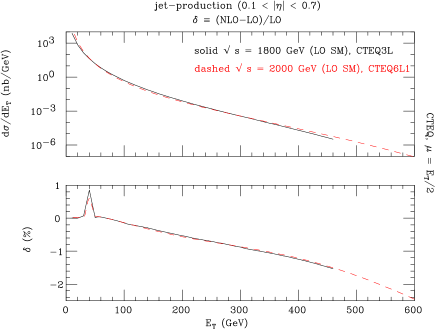
FIG. 1.: The effects of the ${\cal O}(\alpha_{\mathrm{S}}^{2}\alpha_{\mathrm{W}})$ corrections relative to the LO SM results for Run 1(Run 2) using CTEQ3L(CTEQ6L1) as PDFs.

Fig. 1 shows the effects of our one-loop corrections to the LO results for jet production, the latter being defined as including all possible terms of order $\alpha_{\mathrm{S}}^{2}$, $\alpha_{\mathrm{S}}\alpha_{\mathrm{EW}}$ and $\alpha_{\mathrm{EW}}^{2}$ (hereafter LO SM). (The spike at $E_{T}\approx M_{W}/2,M_{Z}/2$ is a threshold effect in the loop diagrams.) Notice that in our treatment we identify the jets with the partons from which they originate and we adopt here the cut $0.1<|\eta|<0.7$ in pseudorapidity to mimic the CDF detector coverage and the standard jet cone requirement $\Delta R>0.7$ to emulate the jet data selection (although we eventually sum the two- and three-jet contributions). Furthermore, as factorisation and renormalisation scale we use $\mu=\mu_{F}\equiv\mu_{R}=E_{T}/2$ – a choice leading to the best convergence of both NLO [24] and resummed [32] QCD predictions – (where $E_{T}$ is the jet transverse energy) while we adopt CTEQ3L as PDFs [27] for Run 1, a set defined prior to the re-arrangement of the gluon. With respect to the LO SM rates, the ${\cal O}(\alpha_{\mathrm{S}}^{2}\alpha_{\mathrm{W}})$ corrections are not large despite growing steadily with $E_{T}$. For $E_{T}$ values in the vicinity of 420 GeV, the highest point of Run 1 and also the location of the apparent CDF excess, they amount to $-1.5\%$. This effect is not competitive with the positive NLO QCD corrections through ${\cal O}(\alpha_{\rm{S}}^{3})$: see, e.g., Fig. 1 of [24]. In the same figure, we have also shown the ${\cal O}(\alpha_{\mathrm{S}}^{2}\alpha_{\mathrm{W}})$ corrections at Run 2 for the same $\mu$ and the choice CTEQ6L1 of PDFs (one of the newest sets incorporating the above mentioned gluon re-parameterisation). Here, we have also increased the $E_{T}$ values probed, as the larger collider energy has already allowed to collect data some 150 GeV beyond the Run 1 reach. We see that at the higher energy the ${\cal O}(\alpha_{\mathrm{S}}^{2}\alpha_{\mathrm{W}})$ corrections are substantially similar in size and shape to the lower energy case, so that they stretch to $-2\%$ or so near the current kinematic limit (550 GeV or so). (Crossing points between the two curves are induced by the different PDF choice as well as the different numerical value of $\mu$ at the two energies.)

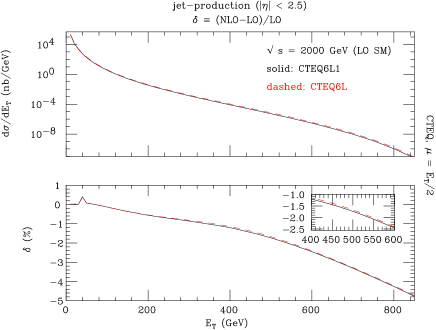
FIG. 2.: The effects of the ${\cal O}(\alpha_{\mathrm{S}}^{2}\alpha_{\mathrm{W}})$ corrections relative to the LO SM results for Run 2 in the presence of two sets of up-to-date PDFs (CTEQ6L and CTEQ6L1).

Fig. 2 extends the $E_{T}$ interval to 850 GeV and the pseudorapidity cover to $|\eta|<2.5$ (our new default from now on, for same $\Delta R$), while still adopting $\mu=E_{T}/2$ as factorisation/renormalisation scale. Including the forward/backward detector region reduces minimally the effects of the ${\cal O}(\alpha_{\mathrm{S}}^{2}\alpha_{\mathrm{W}})$ corrections while their shape remains unchanged. Their maximum is about $-5\%$ at the upper end of the interval considered. Furthermore, their dependence on the choice of PDFs is also very small, as we have verified by running CTEQ6L1 vs. CTEQ6L [27].

Notice however that, if one defines the corrections with respect to only the ${\cal O}(\alpha_{\mathrm{S}}^{2})$ contribution (hereafter, LO QCD), the effects of the sum of all non-QCD terms, i.e., those of order $\alpha_{\mathrm{S}}\alpha_{\mathrm{EW}}$, $\alpha_{\mathrm{EW}}^{2}$ and $\alpha_{\mathrm{S}}^{2}\alpha_{\mathrm{W}}$ (hereafter LO SM + NLO W), become significantly larger. Fig. 3 makes this point clear. At $E_{T}=850$ GeV or so, the upper kinematic limit of the collider, one would see a combined effect of about $-14\%$, most of which are indeed due to the ${\cal O}(\alpha_{\mathrm{S}}^{2}\alpha_{\mathrm{W}})$ terms new to this study (NLO W). In practice though, such jet transverse energies are unreachable even for optimistic luminosity. For the current Run 2 highest $E_{T}$ point, 550 GeV, the effects of the LO SM + NLO W corrections amount to $-8\%$ of the LO QCD term. Clearly, it is of paramount importance to establish which terms are included in Monte Carlo (MC) programs used to interpolate the data. In general, it is clear from Fig. 3 that the corrections due to the one-loop graphs play a role at least as relevant as those due to tree-level effects and, importantly, at Tevatron, they act in the same direction, namely, a reduction of the differential QCD rates.

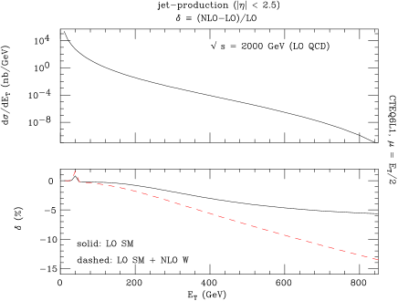
FIG. 3.: The effects of the ${\cal O}(\alpha_{\mathrm{S}}\alpha_{\mathrm{EW}}+\alpha_{\mathrm{EW}}^{2})$ (LO SM) and the latter plus ${\cal O}(\alpha_{\mathrm{S}}^{2}\alpha_{\mathrm{W}})$ (LO SM + NLO W) corrections relative to the LO QCD of ${\cal O}(\alpha_{\mathrm{S}}^{2})$ results for Run 2 in the presence of up-to-date PDFs (CTEQ6L1).

In fact, another subtlety should be borne in mind as far as EW corrections are concerned. We have so far adopted $\mu=E_{T}/2$ for the factorisation/renormalisation scale. This seems in fact to be the preferred choice while comparing Tevatron data against NLO QCD predictions through ${\cal O}(\alpha_{\rm{S}}^{3})$. A discussion of the dependence of the QCD corrections on $\mu$ is found in Refs. [23] –[24] and the above mentioned choice is motivated by the stability of the higher order QCD results in the region $\mu\approx E_{T}/2$. In fact, recall that any dependence on $\mu$ arises because of the truncation of the perturbative expansion at some fixed order and it is therefore a measure of the missing higher order terms. As $\mu$ would not appear if these were known through all orders, it is customary to vary the factorisation/renormalisation scale in order to estimate the residual theoretical error. We have done so in Fig. 4 for, e.g., $E_{T}=100$ and $550$ GeV, at Run 2 energy with CTEQ6L1 as PDFs. The fact that the ${\cal O}(\alpha_{\mathrm{S}}^{2}\alpha_{\mathrm{W}})$ curves do not display local maxima, unlike the ${\cal O}(\alpha_{\mathrm{S}}^{3})$ results (Fig. 2 of [23]), does intimate that one scale choice is not more appropriate than another (irrespective of the jet transverse energy probed and the size of the EW corrections). Thus, there is no firm reason to adopt $E_{T}/2$ as factorisation/renormalisation scale here. If a higher value is chosen at 550 GeV, e.g., $\mu=E_{T}$, the LO SM + NLO W corrections grow of a further percent, to $-9\%$, while for $\mu=2E_{T}$ they become $-10\%$. This trend is manifest over the entire $E_{T}$ range of relevance at Tevatron.

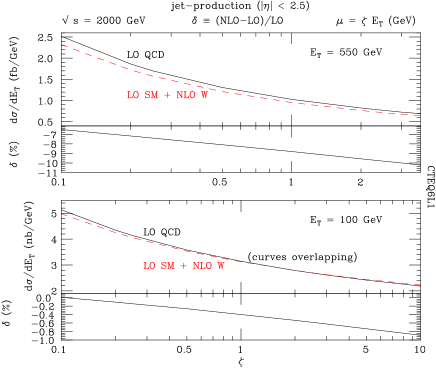
FIG. 4.: The effects of the ${\cal O}(\alpha_{\mathrm{S}}\alpha_{\mathrm{EW}}+\alpha_{\mathrm{EW}}^{2}+\alpha_{\mathrm{S}}^{2}\alpha_{\mathrm{W}})$ (LO SM + NLO W) corrections relative to the LO QCD results as function of $\mu$ for Run 2 in the presence of up-to-date PDFs (CTEQ6L1) for two choices of jet transverse energy.

In summary, at Tevatron, EW effects in general and ${\cal O}(\alpha_{\mathrm{S}}^{2}\alpha_{\mathrm{W}})$ one-loop terms in particular are important contributions to the inclusive jet cross section at large transverse energy. A careful re-analysis of actual jet data, which was beyond the intention of this paper, may be needed in view of the increasing luminosity of the Fermilab collider. Particular care should be devoted to the treatment of real $W$ and $Z$ production and decay in the definition of the inclusive jet data sample, as this will determine whether tree-level $W$ and $Z$ bremsstrahlung effects have to be included in the theoretical predictions through ${\cal O}(\alpha_{\mathrm{S}}^{2}\alpha_{\mathrm{W}})$, which might counterbalance the negative effects due to one-loop $W$ and $Z$ virtual exchange. In closing, we should mention that the calculation of the aforementioned EM effects is in progress.

REFERENCES

- [1] M. Melles, Phys. Rept. 375 (2003) 219.
- [2] A. Denner, arXiv:hep-ph/0110155.
- [3] M. Ciafaloni, P. Ciafaloni and D. Comelli, Phys. Rev. Lett. 84 (2000) 4810, Nucl. Phys. B589 (2000) 359.
- [4] E. Accomando, A. Denner and S. Pozzorini, Phys. Rev. D65 (2002) 073003.
- [5] A. Denner, M. Melles and S. Pozzorini, Nucl. Phys. B662 (2003) 299.
- [6] J. H. Kühn, S. Moch, A. A. Penin and V. A. Smirnov, Nucl. Phys. B616 (2001) 286.
- [7] U. Baur, S. Keller and D. Wackeroth, Phys. Rev. D59 (1999) 013002; U. Baur and D. Wackeroth, Int. J. Mod. Phys. A16S1A (2001) 326, Phys. Rev. D70 (2004) 073015; U. Baur, O. Brein, W. Hollik, C. Schappacher and D. Wackeroth, Phys. Rev. D65 (2002) 033007; S. Dittmaier and M. Krämer, Phys. Rev. D65 (2002) 073007; E. Maina, S. Moretti and D. A. Ross, Phys. Lett. B593 (2004) 143; J. H. Kuhn, A. Kulesza, S. Pozzorini and M. Schulze, arXiv:hep-ph/0408308.
- [8] S. Pozzorini, arXiv:hep-ph/0201077; E. Accomando, A. Denner and A. Kaiser, Nucl. Phys. B706 (2005) 325; W. Hollik and C. Meier, Phys. Lett. B590 (2004) 69.
- [9] E. Maina, S. Moretti, M. R. Nolten and D. A. Ross, Phys. Lett. B570 (2003) 205.
- [10] J. H. Kuhn, A. Scharf and P. Uwer, Eur. Phys. J. C45, 139 (2006).
- [11] W. Bernreuther, M. Fucker and Z. G. Si, Int. J. Mod. Phys. A 21, 914 (2006).
- [12] W. Bernreuther, M. Fuecker and Z. G. Si, Phys. Lett. B 633, 54 (2006).
- [13] S. Moretti, M. R. Nolten and D. A. Ross, arXiv:hep-ph/0603083.
- [14] W. Beenakker, A. Denner, W. Hollik, R. Mertig, T. Sack and D. Wackeroth, Nucl. Phys. B411 (1994) 343.
- [15] C. Kao and D. Wackeroth, Phys. Rev. D61 (2000) 055009.
- [16] M. L. Ciccolini, S. Dittmaier and M. Kramer, Phys. Rev. D68 (2003) 073003.
- [17] W. Hollik et al., Acta Phys. Polon. B35 (2004) 2533.
- [18] U. Baur, E. W. N. Glover and A. D. Martin, Phys. Lett. B232 (1989) 519.
- [19] J. R. Ellis, S. Moretti and D. A. Ross, JHEP 0106 (2001) 043.
- [20] S. Moretti, M. R. Nolten and D. A. Ross, arXiv:hep-ph/0509254; C. Buttar et al., arXiv:hep-ph/0604120.
- [21] T. Affolder et al. [CDF Collaboration], Phys. Rev. D64 (2001) 032001 [Erratum-ibid. D65 (2002) 039903].
- [22] F. Aversa, P. Chiappetta, M. Greco and J. P. Guillet, Phys. Lett. B210 (1988) 225; F. Aversa, M. Greco, P. Chiappetta and J. P. Guillet, Phys. Lett. B211 (1988) 465; F. Aversa, P. Chiappetta, M. Greco and J. P. Guillet, Nucl. Phys. B327 (1989) 105.
- [23] S. D. Ellis, Z. Kunszt and D. E. Soper, Phys. Rev. Lett. 64 (1990) 2121.
- [24] W. T. Giele, E. W. N. Glover and D. A. Kosower, Phys. Rev. Lett. 73 (1994) 2019.
- [25] D. Stump, J. Huston, J. Pumplin, W. K. Tung, H. L. Lai, S. Kuhlmann and J. F. Owens, JHEP 0310 (2003) 046.
- [26] A. D. Martin, R. G. Roberts, W. J. Stirling and R. S. Thorne, Phys. Lett. B604 (2004) 61; M. Klasen and G. Kramer, Phys. Lett. B 386 (1996) 384.
- [27] J. Pumplin, D. R. Stump, J. Huston, H. L. Lai, P. Nadolsky and W. K. Tung, JHEP 0207 (2002) 012.
- [28] http://www-cdf.fnal.gov/physics/new/qcd/inclusive/; http://www-d0.fnal.gov/Run2Physics/qcd/.
- [29] J. A. M. Vermaseren, arXiv:math-ph/0010025.
- [30] J. Küblbeck, M. Böhm and A. Denner, Comput. Phys. Commun. 60 (1990) 165.
- [31] S. Catani and M. H. Seymour, Nucl. Phys. B485 (1997) 291 [Erratum-ibid. B510 (1997) 503].
- [32] N. Kidonakis and J. F. Owens, Phys. Rev. D63 (2001) 054019.