The Pattern of CP Asymmetries in $b\to s$ Transitions

Abstract

New CP violating physics in $b\to s$ transitions will modify the CP asymmetries in $B$ decays into final CP eigenstates ($\phi K_{S}$, $\eta^{\prime}K_{S}$, $\pi^{0}K_{S}$, $\omega K_{S}$, $\rho^{0}K_{S}$ and $\eta K_{S}$) from their Standard Model values. In a model independent analysis, the pattern of deviations can be used to probe which Wilson coefficients get a significant contribution from the new physics. We demonstrate this idea using several well-motivated models of new physics, and apply it to current data.

I Introduction

CP asymmetries in the decays of neutral $B$ mesons into final CP eigenstates $f$ exhibit a time-dependent behavior (for a review of CP violation in meson decays, see Eidelman:2004wy ),

$${\cal A}_{f}(t)=S_{f}\sin(\Delta mt)-C_{f}\cos(\Delta mt).$$ (1)

The Standard Model predicts that for most of the decays that proceed via the quark transitions $\bar{b}\to\bar{q}^{\prime}q^{\prime}\bar{s}$ ($q^{\prime}=c,s,d,u$), the following relations hold to a good approximation:

$$-\eta_{f}S_{f}\simeq\sin 2\beta,\ \ \ \ C_{f}\simeq 0,$$ (2)

where $\eta_{f}=\pm 1$ is the CP eigenvalue for the final state $f$, and $\beta\equiv\phi_{1}\equiv\arg\left[-(V_{cd}V_{cb}^{*})/(V_{td}V_{tb}^{*})\right]$. New physics effects can appear in two ways. First, new physics in ${\cal H}_{\Delta B=2}$ contributes to the $B^{0}-\overline{B}^{0}$ mixing amplitude. Such a contribution shifts all $S_{f}$’s in a universal way: The $S_{f}$ asymmetries remain equal to each other, though different from $\sin 2\beta$. The $C_{f}$’s still vanish. Second, new physics in ${\cal H}_{\Delta B=1}$ can contribute to the $\bar{b}\to\bar{q}q\bar{s}$ transitions ($q=s,d,u$) history . (The tree level transition $\bar{b}\to\bar{c}c\bar{s}$ is unlikely to get a significant contribution from new physics, and consequently the asymmetries $S_{\psi K}$ and $C_{\psi K}$ would not be modified by ${\cal H}_{\Delta B=1}$.) Such a contribution would lead to interesting consequences:

1. The $S_{f}$’s would be different from each other and from $S_{\psi K}$.

2. The $C_{f}$’s would be different from each other and from zero.

Thus, in the presence of new physics, a pattern of deviations, $\delta S_{f}=-\eta_{f}S_{f}-S_{\psi K}\neq 0$ and $C_{f}\neq 0$, will arise.

Given a set of experimental ranges for $\delta S_{f}$ and $C_{f}$, one would like to interpret these data in terms of new physics. There are two ways to proceed. First, one can choose a model of new physics and analyze whether the model can accommodate the data. The second way is model independent. The effects of new physics can be described by a modification of the Wilson coefficients in the operator product expansion for $\Delta B=1$ interactions. Thus, one can fit a set of Wilson coefficients to the data and learn which operators can account for the observed deviations. In this paper, we study this second, model independent, method.

While our analysis has the advantage of being model independent, it suffers from two limitations:

• The number of Wilson coefficients is larger than the number of measured CP asymmetries. Consequently, an analysis that is entirely generic is impossible to carry out at present. Hence, one has to assume that only a subset of all possible operators are modified. In this work we consider some simple cases, where the new physics is parameterized by a single complex parameter. The cases that we study are motivated by actual models of new physics. Extensions to a larger number of new physics parameters is left for future work. It is also possible to include in the analysis additional data, beyond the CP asymmetries in decays into final CP eigenstates. This extension is also left for future work.

• To interpret the data in terms of Wilson coefficients, one has to know the values of the (mode-dependent) hadronic matrix elements of the operators. At present, there is no first principle calculation of the matrix elements that has been tested to a high level of precision. Thus, hadronic uncertainties prevent a clean theoretical interpretation. We use factorization Beneke:2000ry ; Ali:1998eb ; Beneke:2002jn for our analysis.

A number of relevant measurements exists already. The experimental situation is summarized in Table 1.

Table 1: World averages of the experimental results for the CP asymmetries in neutral $B$ decays via the quark transitions $\bar{b}\to\bar{q}^{\prime}q^{\prime}\bar{s}$ modes, $q^{\prime}=c,s,d,u$.

$f$	$-\eta_{\rm CP}S_{f}$	$C_{f}$	Refs.
$\psi K_{S}$	$+0.73\pm 0.04$	$+0.03\pm 0.03$	Abe:2004mz ; Aubert:2004zt
$\phi K_{S}$	$+0.35\pm 0.21$	$-0.04\pm 0.17$	Aubert:2005ja ; Abe:2004xp
$\eta^{\prime}K_{S}$	$+0.43\pm 0.11$	$-0.04\pm 0.08$	Aubert:2005iy ; Abe:2004xp
$\pi^{0}K_{S}$	$+0.34\pm 0.29$	$+0.08\pm 0.14$	Aubert:2005zt ; Abe:2004xp
$\omega K_{S}$	$+0.56\pm 0.32$	$-0.49\pm 0.25$	Abe:2004xp ; Aubert:2005ra

The plan of this paper is as follows. In section II we introduce our formalism and evaluate, to leading log approximation and within the QCD factorization approach, the Standard Model (SM) predictions for the CP asymmetries. In section III we analyze the effects of new physics. We start with a generic, model independent analysis, using the operator product expansion for $\Delta B=1$ operators. We then focus on scenarios where the effects of new physics depend on a single complex parameter. We give three explicit examples of such scenarios. In section IV we apply our approach to present data. We conclude in section V.

II Formalism and Standard Model Predictions

We follow the notations of ref. Beneke:2000ry . We consider the following effective Hamiltonian for $\Delta B=\pm 1$ decays:

$${\cal H}_{\rm eff}={G_{F}\over\sqrt{2}}\sum_{p=u,c}V_{ps}^{*}V_{pb}\left(C_{1}O_{1}^{p}+C_{2}O_{2}^{p}+\sum_{i=3}^{10}C_{i}O_{i}+C_{7\gamma}O_{7\gamma}+C_{8g}O_{8g}\right)+{\rm h.c.},$$ (3)

with

$$O_{1}^{p}=(\bar{p}b)_{V-A}(\bar{s}p)_{V-A}, O_{2}^{p}=(\bar{p}_{\beta}b_{\alpha})_{V-A}(\bar{s}_{\alpha}p_{\beta})_{V-A},$$

$$O_{3}=(\bar{s}b)_{V-A}\sum_{q}(\bar{q}q)_{V-A}, O_{4}=(\bar{s}_{\alpha}b_{\beta})_{V-A}\sum_{q}(\bar{q}_{\beta}q_{\alpha})_{V-A},$$

$$O_{5}=(\bar{s}b)_{V-A}\sum_{q}(\bar{q}q)_{V+A}, O_{6}=(\bar{s}_{\alpha}b_{\beta})_{V-A}\sum_{q}(\bar{q}_{\beta}q_{\alpha})_{V+A},$$

$$O_{7}=\frac{3}{2}(\bar{s}b)_{V-A}\sum_{q}e_{q}(\bar{q}q)_{V+A}, O_{8}=\frac{3}{2}(\bar{s}_{\alpha}b_{\beta})_{V-A}\sum_{q}e_{q}(\bar{q}_{\beta}q_{\alpha})_{V+A},$$

$$O_{9}=\frac{3}{2}(\bar{s}b)_{V-A}\sum_{q}e_{q}(\bar{q}q)_{V-A}, O_{10}=\frac{3}{2}(\bar{s}_{\alpha}b_{\beta})_{V-A}\sum_{q}e_{q}(\bar{q}_{\beta}q_{\alpha})_{V-A},$$

$$O_{7\gamma}=-\frac{em_{b}}{8\pi^{2}}\bar{s}\sigma^{\mu\nu}(1+\gamma_{5})F_{\mu\nu}b, O_{8g}=-\frac{g_{s}m_{b}}{8\pi^{2}}\bar{s}\sigma^{\mu\nu}(1+\gamma_{5})G_{\mu\nu}b,$$ (4)

where $(\bar{q}_{1}q_{2})_{V\pm A}=\bar{q}_{1}\gamma_{\mu}(1\pm\gamma_{5})q_{2}$, the sum is over active quarks, with $e_{q}$ denoting their electric charge in fractions of $|e|$ and $\alpha,\beta$ are color indices.

The CP asymmetries in $B\to f$ decays are calculated as follows. One defines a complex quantity $\lambda_{f}$,

$$\lambda_{f}=e^{-i\phi_{B}}(\overline{A}_{f}/A_{f}),$$ (5)

where $\phi_{B}$ is the phase of $M_{12}$, the $B^{0}-\overline{B}^{0}$ mixing amplitude, and $A_{f}$ ($\overline{A}_{f}$) is the decay amplitude for $B^{0}(\overline{B}^{0})\to f$. We have

$$S_{f}=\frac{2{\cal I}m(\lambda_{f})}{1+|\lambda_{f}|^{2}},\ \ \ C_{f}=\frac{1-|\lambda_{f}|^{2}}{1+|\lambda_{f}|^{2}}.$$ (6)

The decay amplitudes can be calculated from the effective Hamiltonian of eq. (3) Ali:1998eb :

$$A_{f}=\langle f|{\cal H}_{\rm eff}|B^{0}\rangle,\ \ \ \overline{A}_{f}=\langle f|{\cal H}_{\rm eff}|\overline{B}^{0}\rangle.$$ (7)

The electroweak model determines the Wilson coefficients while QCD (or, more practically, a calculational method such as QCD factorization) determines the matrix elements $\langle f|O_{i}|B^{0}(\overline{B}^{0})\rangle$.

We perform our calculations to leading-log approximation. In particular, to run the Wilson coefficients from the weak scale $m_{W}$ to a low scale of order $m_{b}$, we use the 12-dimensional leading-log anomalous dimension matrix $\gamma$ Buchalla:1995vs that is given in Table 2. The $\alpha_{s}$ mixing of electroweak penguins onto the dipole operators is deduced from Buchalla:1995vs ; Chetyrkin:1997gb ; Baranowski:1999tq .

Table 2: The anomalous dimension matrix at leading log. The rows and columns correspond to the twelve operators $O_{1,\ldots,10,7\gamma,8g}$ defined in eq. (II).

$-2$	6	$-\frac{2}{9}$	$\frac{2}{3}$	$-\frac{2}{9}$	$\frac{2}{3}$	$0$	$0$	$0$	$0$	$\frac{416}{81}$	$\frac{70}{27}$
6	$-2$	0	0	0	0	0	0	0	0	0	3
$0$	$0$	$-\frac{22}{9}$	$\frac{22}{3}$	$-\frac{4}{9}$	$\frac{4}{3}$	$0$	$0$	$0$	$0$	$-\frac{464}{81}$	$\frac{545}{27}$
$0$	$0$	$\frac{44}{9}$	$\frac{4}{3}$	$-\frac{10}{9}$	$\frac{10}{3}$	$0$	$0$	$0$	$0$	$\frac{136}{81}$	$\frac{512}{27}$
$0$	$0$	$0$	$0$	$2$	$-6$	$0$	$0$	$0$	$0$	$\frac{32}{9}$	$-\frac{59}{3}$
$0$	$0$	$-\frac{10}{9}$	$\frac{10}{3}$	$-\frac{10}{9}$	$-\frac{38}{3}$	$0$	$0$	$0$	$0$	$-\frac{296}{81}$	$-\frac{703}{27}$
$0$	$0$	$0$	$0$	$0$	$0$	$2$	$-6$	$0$	$0$	$-\frac{16}{9}$	$\frac{5}{6}$
$0$	$0$	$-\frac{1}{9}$	$\frac{1}{3}$	$-\frac{1}{9}$	$\frac{1}{3}$	$0$	$-16$	$0$	$0$	$-\frac{1196}{81}$	$-\frac{11}{54}$
$0$	$0$	$\frac{2}{9}$	$-\frac{2}{3}$	$\frac{2}{9}$	$-\frac{2}{3}$	$0$	$0$	$-2$	$6$	$\frac{232}{81}$	$-\frac{59}{54}$
$0$	$0$	$-\frac{1}{9}$	$\frac{1}{3}$	$-\frac{1}{9}$	$\frac{1}{3}$	$0$	$0$	$6$	$-2$	$\frac{1180}{81}$	$-\frac{46}{27}$
$0$	$0$	$0$	$0$	$0$	$0$	$0$	$0$	$0$	$0$	$\frac{32}{3}$	$0$
$0$	$0$	$0$	$0$	$0$	$0$	$0$	$0$	$0$	$0$	$-\frac{32}{9}$	$\frac{28}{3}$

Within the SM, we have the following set of Wilson coefficients at leading order:

$$C_{1}^{\rm SM}(m_{W})=1,\ \ \ C_{i\neq 1}^{\rm SM}(m_{W})=0.$$ (8)

(Strictly speaking, $C_{7\gamma}^{\rm SM}(m_{W})$ and $C_{8g}^{\rm SM}(m_{W})$ are also different from zero. However, their contributions to the decay processes of interest occur at next-to-leading order which we neglect in the present work.) The SM contribution to the decay amplitudes, related to $\bar{b}\to\bar{q}^{\prime}q^{\prime}\bar{s}$ transitions, can always be written as a sum of two terms, $A_{f}^{\rm SM}=A_{f}^{c}+A_{f}^{u}$, with $A_{f}^{c}\propto V_{cb}^{*}V_{cs}$ and $A_{f}^{u}\propto V_{ub}^{*}V_{us}$. Defining the ratio $a_{f}^{u}\equiv e^{-i\gamma}(A_{f}^{u}/A_{f}^{c})$, where $\gamma\equiv\phi_{3}\equiv\arg\left[-(V_{ud}V_{ub}^{*})/(V_{cd}V_{cb}^{*})\right]$, we have

$$A_{f}^{\rm SM}=A_{f}^{c}\left(1+a_{f}^{u}e^{i\gamma}\right).$$ (9)

For $B\to\psi K_{S}$, the $a_{f}^{u}$ term can be safely neglected (its effects are below the percent level) and, consequently,

$$\lambda_{\psi K_{S}}^{\rm SM}=-e^{-2i\beta}.$$ (10)

For charmless modes, the effects of the $a_{f}^{u}$ terms (often called ‘the SM pollution’) are at least of order $|(V_{ub}V_{us}^{*})/(V_{cb}V_{cs}^{*})|\sim$ a few percent. They can lead to a deviation of $S_{f}$ from $S_{\psi K}$ and of $C_{f}$ from zero. In Table 3 we give the values of the $a_{f}^{u}$ parameter (obtained, as explained above, by using factorization Beneke:2000ry ; Ali:1998eb ; Beneke:2002jn ) for all relevant modes. Since we perform our calculations to leading log approximation, we neglect, for consistency, also power corrections within the QCD factorization approach, except for the dominant chirally-enhanced ones related to $a_{6}$ and $a_{8}$. This means that the strong phases vanish, and that $C_{f}=0$ for all $f$ in this approximation. The SM predictions for $S_{f}$ (with $S_{\psi K_{S}}=0.73$ and $\gamma=62^{o}$ Charles:2004jd taken as input) are also given in Table 3. The values of the input parameters used are specified in Table 4. To estimate our uncertainties, we give the values for $\mu=m_{b}=4.2$ GeV and for a varied renormalization scale of $\mu=m_{b}/2$ and $\mu=2m_{b}$. Note that the coefficients of the chirally enchanced terms, defined as $r_{\chi}=2m_{K}^{2}/(m_{b}m_{s})$ and $r_{\chi}^{S_{s}}=h_{S}^{s}/(f_{S}^{s}m_{b}m_{s})$ for the singlets $S=\eta,\eta^{\prime}$ (see Beneke:2002jn for details), evolve with the renormalization scale through the running ($\overline{\rm MS}$-bar) quark masses.

Table 3: The $a_{f}^{u}$ parameters, calculated in QCD factorization at leading log and to zeroth order in $\Lambda/m_{b}$ (except for chirally enhanced corrections), and the SM values of $S_{f}$ for $\mu=m_{b}$ and in parentheses the respective values for $\mu=2m_{b}$ (first) and $\mu=m_{b}/2$ (second) if different from the central one.

$f$	$a_{f}^{u}$	$-\eta_{\rm CP}S_{f}$
$\psi K_{S}$	$0$	$0.73$
$\phi K_{S}$	$0.019$	$0.75$
$\pi^{0}K_{S}$	$0.052\,\left[0.094,0.021\right]$	$0.79\,\left[0.83,0.76\right]$
$\eta K_{S}$	$0.08\,\left[0.16,0.02\right]$	$0.82\,\left[0.88,0.76\right]$
$\eta^{\prime}K_{S}$	$0.007\,\left[-0.006,0.019\right]$	$0.74\,\left[0.72,0.75\right]$
$\omega K_{S}$	$0.22\,\left[0.37,0.04\right]$	$0.92\,\left[0.98,0.78\right]$
$\rho^{0}K_{S}$	$-0.16\,\left[-0.32,0.005\right]$	$0.49\,\left[0.19,0.74\right]$

Table 4: Input parameters used in the calculations.

Decay constants (MeV)			Form Factors			$r_{\chi}$-factors, quark masses
$f_{\pi}$	$131$		$F^{B\to\pi}(0)$	$0.28$
$f_{K}$	$160$		$F^{B\to K}(0)$	$0.34$		$r_{\chi}(m_{b})$	$1.170$
$f^{q}_{\eta}$	$108$		$F^{B\to\eta}(0)$	$0.23$		$r_{\chi}^{\eta_{s}}(m_{b})$	$1.230$
$f^{s}_{\eta}$	$-111$
$f^{q}_{\eta^{\prime}}$	$89$		$F^{B\to\eta^{\prime}}(0)$	$0.19$		$r_{\chi}^{\eta^{\prime}_{s}}(m_{b})$	$1.241$
$f^{s}_{\eta^{\prime}}$	$136$					$m_{b}(m_{b})$	4.2 GeV
$f_{\omega}$	$187$		$A^{B\to\omega}(0)$	$0.33$		$m_{s}$(2GeV)	110 MeV
$f_{\rho}$	$209$		$A^{B\to\rho}(0)$	$0.37$		$(m_{u}+m_{d})$(2GeV)	9.1 MeV

An examination of Table 3 shows that the SM pollution is small (that is, at the naively expected level of $|(V_{ub}V_{us}^{*})/(V_{cb}V_{cs}^{*})|\sim$ a few percent) for $f=\phi K_{S},\ \eta^{\prime}K_{S}$ and $\pi^{0}K_{S}$. It is larger for $f=\eta K_{S},\ \omega K_{S}$ and $\rho^{0}K_{S}$. In these modes, $a_{f}^{u}$ is enhanced because, within the QCD factorization approach, there is an accidental cancellation between the leading contributions to $A_{f}^{c}$. The reason for the suppression of the leading $A^{c}_{f}$ piece in $f=\rho K,\ \omega K$ versus $f=\pi^{0}K$ is that the dominant QCD-penguin coefficients $a_{4}$ and $a_{6}$ appear in $A_{(\rho,\omega)K}^{c}$ as $(a_{4}-r_{\chi}a_{6})$ and in $A^{c}_{\pi^{0}K}$ as $(a_{4}+r_{\chi}a_{6})$. Since $r_{\chi}\simeq 1$ and, within the Standard Model, $a_{4}\sim a_{6}$, there is a cancellation in $A_{(\rho,\omega)K}^{c}$ while there isn’t one in $A^{c}_{\pi^{0}K}$. The suppression for $A^{c}_{\eta K}$ with respect to $A^{c}_{\eta^{\prime}K}$ has a different reason: it is due to the octet-singlet mixing, which causes destructive (constructive) interference in the $\eta(\eta^{\prime})K$ penguin amplitude Lipkin:1980tk .

We stress that the numerical results presented above are often sensitive to the approximations that we make and to the values of the input parameters. We will refine them in the future by going beyond the leading log approximation and taking into account uncertainties in the input parameters other than the scale $\mu$. At present they should be taken as indication to how close to $S_{\psi K_{S}}$ one should expect the various $S_{f}$’s to be, but not as accurate predictions. Our findings are compatible with the next to leading order results in the SM given by MartinCKM2005talk .

We conclude this section by adding some general considerations concerning the accuracy of our approximation and the stability of our results. We discuss two main points. First, the validity of our approximation for branching ratios and direct CP asymmetries. Second, the presence of large power corrections in our analysis.

Regarding the first issue, there is a substantial effect from NLO corrections in factorization as far as the branching ratios are concerned. However, the impact of such NLO corrections is very moderate for the asymmetries $S_{f}$, which are the main focus of our study. This can be demonstrated explicitly in the SM by comparing our results (Table 3) with the more complete, full-fledged NLO analysis of MartinCKM2005talk . In fact, even the estimate of theoretical uncertainties, which we obtained by a variation of the renormalization scale, is in good agreement with MartinCKM2005talk , where also other sources of uncertainty are included. This clearly demonstrates that our approach gives a reasonable picture for the asymmetries $S_{f}$, including the issue of uncertainties and the stability against subleading effects.

In addition, our framework is still consistent with the observed direct CP asymmetries $C_{f}$, which are compatible with zero. This is the case in general for direct CP asymmetries in all $B$ decays, where $A_{CP}(K^{+}\pi^{-})$ is so far the only exception. Even in this case the observed direct CP asymmetry is not very large (about $10\%$).

Regarding the second issue, we stress again in this context that the dominant power corrections related to $Q_{6}$ and $Q_{8}$ are included in our analysis (as already mentioned in footnote 1). Further power corrections, in particular those from annihilation topologies can be estimated Beneke:2000ry to be typically of the order $10$ - $20\%$ with respect to the factorizable prediction. Hence the impact of such effects is subdominant. This is also confirmed by the comparison with MartinCKM2005talk mentioned above.

III New Physics

III.1 Generic analysis

For the purpose of discussing new physics, it is convenient to define a phase $\beta_{\rm eff}$:

$$\lambda_{\psi K_{S}}\equiv-e^{-2i\beta_{\rm eff}}.$$ (11)

In writing down eq. (11), we are making the very plausible assumption that the quark transition $b\to c\bar{c}s$ is dominated by a single weak phase. This is clearly the case within the SM, where the phase of $V_{cb}V_{cs}^{*}$ dominates to better than one percent. But even with new physics we do not expect significant new contributions to SM tree level processes. The approximation of a single weak phase may be not as good as in the SM, but it is still expected to be a very good approximation. On the other hand, eq. (11) allows for new physics in $B^{0}-\overline{B}^{0}$ mixing, in which case $\beta_{\rm eff}\neq\beta$.

Contributions of new physics to ${\cal H}_{\rm eff}$ of eq. (3) modify the Wilson coefficients $C_{i}$. (New physics can also introduce additional operators. We do not consider this possibility here, but our analysis can be generalized to this case in a straightforward manner.) This modification can be parametrized as follows:

$$C_{i}(m_{W})=C_{i}^{\rm SM}(m_{W})+\varepsilon_{i}e^{i\theta_{i}},$$ (12)

where $C_{i}^{\rm SM}$ is the Standard Model value of the Wilson coefficient, $\varepsilon_{i}$ is real and positive, and $\theta_{i}$ is a phase in the range $[0,2\pi]$.

The modification of $A_{f}$ from the SM expression [eq. (9)] due to the new physics contribution [eq. (12)] can always be written as follows:

$$A_{f}=A_{f}^{c}\left[1+a_{f}^{u}e^{i\gamma}+\sum_{i}\left(b_{fi}^{c}+b_{fi}^{u}e^{i\gamma}\right)\varepsilon_{i}e^{i\theta_{i}}\right].$$ (13)

In Table 5, we give the values of the $b_{fi}^{c}$ parameters within the QCD factorization approach Beneke:2000ry ; Ali:1998eb ; Beneke:2002jn . The $b_{fi}^{u}$ for $i=3,\ldots,10$ are related to the $b_{fi}^{c}$ through $b^{u}_{fi}=(|V_{ub}V_{us}^{*}|/|V_{cb}V_{cs}^{*}|)\,b^{c}_{fi}$. Note that further $b_{f1}^{c}=1$ and $b_{f1}^{u}=a^{u}_{f}$.

Table 5: The $b_{fi}^{c}$ ($i=1,\ldots,10$) and $b_{f1,2}^{u}$ parameters calculated in QCD factorization to leading log approximation at $\mu=m_{b}$ and to zeroth order in $\Lambda/m_{b}$ (except for chirally enhanced corrections).

$f$	$\pi^{0}K$	$\eta K$	$\eta^{\prime}K$	$\phi K$	$\omega K$	$\rho^{0}K$
$b_{f1}^{c}$	$1$	$1$	$1$	$1$	$1$	$1$
$b_{f1}^{u}$	$0.052$	$0.08$	$0.0072$	$0.019$	$0.22$	$-0.16$
$b_{f2}^{c}$	$-0.12$	$-0.11$	$-0.13$	$-0.13$	$-0.096$	$-0.093$
$b_{f2}^{u}$	$0.32$	$0.59$	$-0.12$	$-0.0024$	$1.9$	$-1.8$
$b_{f3}^{c}$	$-0.34$	$17$	$-26$	$-46$	$210$	$9.3$
$b_{f4}^{c}$	$-12$	$-7.4$	$-17$	$-43$	$110$	$81$
$b_{f5}^{c}$	$-12$	$-28$	$12$	$-43$	$140$	$-55$
$b_{f6}^{c}$	$-31$	$-39$	$-21$	$-20$	$-51$	$-160$
$b_{f7}^{c}$	$-19$	$-32$	$3.8$	$22$	$80$	$-110$
$b_{f8}^{c}$	$3.6$	$-5.1$	$20$	$14$	$120$	$-1.6$
$b_{f9}^{c}$	$25$	$37$	$3.5$	$23$	$45$	$-140$
$b_{f10}^{c}$	$12$	$11$	$11$	$24$	$-36$	$-51$

With new physics, the deviation of $S_{f}$ of charmless modes from $S_{\psi K}$ depends on $b_{fi}^{c}$, $b_{fi}^{u}$, $\varepsilon_{i}$ and $\theta_{i}$. If enough measurements of $S_{f}$ and $C_{f}$ asymmetries become available, one will be able to find the values of the $\varepsilon_{i}$- and $\theta_{i}$- parameters that account for the data. Given a small set of measurements, one can still find $\varepsilon_{i}$ and $\theta_{i}$ if only a small number of operators is affected by the new physics in a significant way. In the next section, we focus on a simple (but well motivated) case in which the contribution of the new physics can be parametrized in terms of a single complex parameter.

III.2 A single complex parameter

Suppose that all the $\varepsilon_{i}e^{i\theta_{i}}$ parameters of eq. (12) are related to a single complex parameter, that is,

$$\varepsilon_{i}e^{i\theta_{i}}=x_{i}\varepsilon e^{i\theta}\ {\rm for\ all}\ i,$$ (14)

where, in a given model of new physics, the $x_{i}$-constants are computable (see section III.3 for three specific examples). In such cases, eq. (13) takes the following form:

$$A_{f}=A_{f}^{c}\left[1+a_{f}^{u}e^{i\gamma}+\left(b_{f}^{c}+b_{f}^{u}e^{i\gamma}\right)\varepsilon e^{i\theta}\right].$$ (15)

The analysis is simpler if $|b_{f}^{c}|\gg|b_{f}^{u}|$. This is the case for all generic combinations of operators $O_{i}$ in eq. (II) that do not involve $i=1,2$. We proceed therefore in discussing the case where a combination of operators within the set $i=3,\ldots,10,7\gamma,8g$ is affected by new physics. For two classes of interesting scenarios, simple analytical expressions can be obtained for the modification of $S_{f}$ and $C_{f}$.

(i) The new physics contribution is dominant. Explicitly,

$$\varepsilon|b_{f}^{c}|\gg|a_{f}^{u}|,1.$$ (16)

The shift in all modes where eq. (16) holds is universal and depends only on $\theta$:

$$-\eta_{f}S_{f} \simeq \sin 2\beta_{\rm eff}\cos 2\theta+\cos 2\beta_{\rm eff}\sin 2\theta,$$

$$C_{f} \simeq 0.$$ (17)

(ii) The new physics contribution and the SM pollution are small. Explicitly,

$$\varepsilon|b_{f}^{c}|\ll 1\ {\rm and}\ |a_{f}^{u}|\ll 1.$$ (18)

The shift is mode dependent and depends on $\varepsilon\sin\theta$:

$$-\eta_{f}S_{f} \simeq \sin 2\beta_{\rm eff}+2\cos 2\beta_{\rm eff}\left[{\cal R}e(b_{f}^{c})\varepsilon\sin\theta+{\cal R}e(a_{f}^{u})\sin\gamma\right],$$

$$C_{f} \simeq -2{\cal I}m(b_{f}^{c})\varepsilon\sin\theta-2{\cal I}m(a_{f}^{u})\sin\gamma.$$ (19)

Since the $b_{f}^{c}$ values are known (see Table 5), the pattern of deviations is predicted and can be used, by comparing with the data, to close in on the set of operators that is responsible for the deviations and to extract $\varepsilon\sin\theta$.

In case that none of these approximations applies, one can still find the pattern of deviations by numerical evaluation for any values for $\varepsilon$ and $\theta$. By comparing these theoretical $\delta S_{f}$ and $C_{f}$ to the data, allowed regions in the $\varepsilon-\theta$ plane (for each scenario) can be determined, and a best fit point (among all scenarios) can be found. We demonstrate this procedure in the next section by using present data.

III.3 Specific Scenarios

We now consider three explicit examples of new physics models. All three examples are well motivated and fulfill eq. (14).

(i) The dominant effect of the new physics is through $Z$-penguins Atwood:2003tg . Then, the Wilson coefficients are modified as follows:

$$C_{3}^{\rm NP}(m_{W}) = \frac{1}{6}\varepsilon_{z}e^{i\theta_{z}},$$

$$C_{7}^{\rm NP}(m_{W}) = \frac{2}{3}\sin^{2}\theta_{W}\varepsilon_{z}e^{i\theta_{z}},$$

$$C_{9}^{\rm NP}(m_{W}) = -\frac{2}{3}(1-\sin^{2}\theta_{W})\varepsilon_{z}e^{i\theta_{z}}.$$ (20)

Here

$$\varepsilon_{z}e^{i\theta_{z}}=\frac{g^{2}}{4\pi^{2}}\frac{Z_{sb}}{V_{tb}V_{ts}^{*}},$$ (21)

where $Z_{sb}$ parametrizes the coupling of the $Z^{0}$ boson to the left handed strange and bottom quarks. The consistency of the measured BR$(b\to s\ell^{+}\ell^{-})$ with the SM prediction requires that $|Z_{sb}|\leq 0.08$ Atwood:2003tg which gives

$$\varepsilon_{z}\mathrel{\hbox to0.0pt{\lower 4.0pt\hbox{\hskip 1.0pt$\sim$}\hss}\raise 1.0pt\hbox{$<$}}0.02.$$ (22)

(ii) Kaluza-Klein excitations of gluons in RS models Burdman:2003nt couple mainly to the third generation quarks and contribute to all gluonic penguin operators:

$$C_{4}^{\rm NP}(m_{W}) = C_{6}^{\rm NP}(m_{W})=\varepsilon_{k}e^{i\theta_{k}},$$

$$C_{3}^{\rm NP}(m_{W}) = C_{5}^{\rm NP}(m_{W})=-\frac{1}{3}\varepsilon_{k}e^{i\theta_{k}}.$$ (23)

Here

$$\varepsilon_{k}e^{i\theta_{k}}=-\pi\alpha_{s}(M_{G})\left(\frac{v}{M_{G}}\right)^{2}\frac{D_{sb}}{V_{tb}V_{ts}^{*}}\chi,$$ (24)

where $D_{sb}$ is the rotation matrix from interaction to mass basis for the left-handed down quarks, $\chi={\cal O}(1)$ is a model dependent parameter (related to bulk fermion masses), and $M_{G}$ is the mass of the lightest excitation. With $M_{G}\mathrel{\hbox to0.0pt{\lower 4.0pt\hbox{\hskip 1.0pt$\sim$}\hss}\raise 1.0pt\hbox{$>$}}1\ TeV$ and $|D_{sb}|\sim|V_{tb}V_{ts}^{*}|$, we expect

$$\varepsilon_{k}\mathrel{\hbox to0.0pt{\lower 4.0pt\hbox{\hskip 1.0pt$\sim$}\hss}\raise 1.0pt\hbox{$<$}}0.02.$$ (25)

(iii) Enhanced chromomagnetic operator Kagan:1997sg can be parametrized as follows:

$$C_{8g}^{\rm NP}(m_{W})=\varepsilon_{g}e^{i\theta_{g}}.$$ (26)

(We still make the approximation that $C_{8g}^{\rm SM}(m_{W})=0$ and neglect further $C_{8g}^{\rm SM}(m_{b})$ induced by $O_{1}$.) From BR($B\to X_{s}g)<0.09$ Coan:1997ye ; Kagan:1997sg , we have

$$\varepsilon_{g}\mathrel{\hbox to0.0pt{\lower 4.0pt\hbox{\hskip 1.0pt$\sim$}\hss}\raise 1.0pt\hbox{$<$}}1.$$ (27)

Note that in this case the new physics contribution enters at next to leading order. Yet, the modifications of the CP asymmetries can be substantial. An experimental improvement by a factor of a few in the upper bound on BR($B\to X_{s}g)$ will restrict the potential modifications in this scenario in a significant way.

We have calculated the $b_{f}^{c}$ and $b_{f}^{u}$ parameters of eq. (15) for each of the three scenarios. We use the factorized decay amplitudes from Beneke:2000ry ; Ali:1998eb ; Beneke:2002jn . (We use asymptotic distribution amplitudes in the analysis of the scenario with an enhanced chromomagnetic operator.) The results are presented in Table 6. The $b_{f}^{c}$ parameters are quite stable under variation of the scale. As anticipated in section III.2, in all three scenarios we have $b^{u}_{f}=(|V_{ub}V_{us}^{*}|/|V_{cb}V_{cs}^{*}|)\,b^{c}_{f}$.

Table 6: The $b_{f}^{c}$ parameters calculated in QCD factorization to leading log approximation and to zeroth order in $\Lambda/m_{b}$ (chirally enhanced corrections are included) in the three scenarios: (i) $Z$-penguins [eq. (III.3)], denoted with subindex $z$; (ii) KK-gluons [eq. (III.3)], denoted with subindex $k$; (iii) Chromomagnetic operator [eq. (26)], denoted with subindex $g$. The first row in each case is obtained for $\mu=m_{b}$, whereas the second row gives the values for $\mu=m_{b}/2$ (first) and $2m_{b}$ (second).

$f$	$\pi^{0}K$	$\eta K$	$\eta^{\prime}K$	$\phi K$	$\omega K$	$\rho^{0}K$
$b_{fz}^{c}$	$-16$	$-21$	$-5.4$	$-16$	$24$	$57$
	$\left[-12,-22\right]$	$\left[-16,-30\right]$	$\left[-4.0,-7.6\right]$	$\left[-10,-24\right]$	$\left[29,28\right]$	$\left[60,65\right]$
$b_{fk}^{c}$	$-39$	$-43$	$-34$	$-33$	$-61$	$-64$
	$\left[-28,-55\right]$	$\left[-33,-59\right]$	$\left[-22,-51\right]$	$\left[-24,-48\right]$	$\left[-63,-74\right]$	$\left[-66,-75\right]$
$b_{fg}^{c}$	$0.75$	$0.64$	$0.86$	$1.4$	$-1.7$	$-1.5$
	$\left[0.61,0.99\right]$	$\left[0.48,0.87\right]$	$\left[0.76,1.07\right]$	$\left[1.1,1.8\right]$	$\left[-2.8,-1.4\right]$	$\left[-2.0,-1.3\right]$

Given the upper bounds on $\varepsilon$ for the three scenarios – $\varepsilon_{z}\mathrel{\hbox to0.0pt{\lower 4.0pt\hbox{\hskip 1.0pt$\sim$}\hss}\raise 1.0pt\hbox{$<$}}0.02$, $\varepsilon_{k}\mathrel{\hbox to0.0pt{\lower 4.0pt\hbox{\hskip 1.0pt$\sim$}\hss}\raise 1.0pt\hbox{$<$}}0.02$ and $\varepsilon_{g}\mathrel{\hbox to0.0pt{\lower 4.0pt\hbox{\hskip 1.0pt$\sim$}\hss}\raise 1.0pt\hbox{$<$}}1$ – we learn that in none of the three examples can the new physics strongly dominate over the SM contributions, that is, $\varepsilon b_{f}^{c}\not\gg a_{f}^{u},1$. Thus, if the data makes a convincing case for a universal pattern of deviations, it would mean that either this pattern is accidental or that the new physics is different from the three specific scenarios discussed here.

On the other hand, the interpretation of the results presented in Table 6 is straightforward in the other limit discussed in the previous subsection. For the four modes $f=\pi^{0}K_{S},\ \eta K_{S},\ \eta^{\prime}K_{S}$ and $\phi K_{S}$, we have, say, $|b_{f}^{c}\varepsilon|\mathrel{\hbox to0.0pt{\lower 4.0pt\hbox{\hskip 1.0pt$\sim$}\hss}\raise 1.0pt\hbox{$<$}}0.3$ for $\varepsilon_{z}\mathrel{\hbox to0.0pt{\lower 4.0pt\hbox{\hskip 1.0pt$\sim$}\hss}\raise 1.0pt\hbox{$<$}}0.01$, $\varepsilon_{k}\mathrel{\hbox to0.0pt{\lower 4.0pt\hbox{\hskip 1.0pt$\sim$}\hss}\raise 1.0pt\hbox{$<$}}0.005$, and $\varepsilon_{g}\mathrel{\hbox to0.0pt{\lower 4.0pt\hbox{\hskip 1.0pt$\sim$}\hss}\raise 1.0pt\hbox{$<$}}0.17$. In any of these cases, the deviation from the SM prediction is proportional to $b_{f}^{c}$ [see eq. (III.2)]. Consequently, there is a distinct pattern of deviations for each of the three scenarios. For example, the deviation of $S_{\eta^{\prime}K_{S}}$ from the SM prediction is a factor of four smaller than that of $S_{\eta K_{S}}$ in the first scenario ($\varepsilon_{z}\neq 0$), a factor $\sim 1.3$ smaller in the second ($\varepsilon_{k}\neq 0$) and a factor of $\sim 1.3$ larger in the third ($\varepsilon_{g}\neq 0$). The deviation of $S_{\phi K_{S}}$ is similar or somewhat smaller than that of $S_{\pi K_{S}}$ in the first two scenarios, but a factor of $\sim 1.9$ larger in the third. The second scenario has the characteristic feature that the SM deviations of $S_{\phi K_{S}}$ and $S_{\eta^{\prime}K_{S}}$ are very similar, whereas in scenario i (iii) $S_{\phi K_{S}}$ is a factor of 3 (1.6) larger than $S_{\eta^{\prime}K_{S}}$. It is interesting to note that in all three new physics examples, the deviations for $b_{f}^{c}\varepsilon\ll 1$ in the modes that have been most accurately measured, $f=\pi^{0}K_{S},\ \eta^{\prime}K_{S}$ and $\phi K_{S}$, and also $\eta K_{S}$, are in the same direction, that is, the four $S_{f}$ asymmetries are either all larger or all smaller [depending on sign($\sin\theta$)] than the SM prediction.

To demonstrate how the pattern of deviations probes new physics, we perform the following exercise. For each of the three scenarios discussed in this section, we take $\varepsilon_{i}$ at the phenomenological upper bound, that is $\varepsilon_{z}=0.02$, $\varepsilon_{k}=0.02$ and $\varepsilon_{g}=1$. Since the new physics contribution is now as large as it can get, the patterns of deviations are expected to be more significant. We then pick the two values of $\theta_{i}$ for which $S_{\pi K_{S}}=0.34$, the experimental central value. (There is no particular reason for selecting $S_{\pi K_{S}}$. Our aim is just to demonstrate the idea that the pattern of deviations is sensitive to new physics.) We present the results in Fig. 1. One can clearly see that the six patterns are different from each other, so that each scenario can in principle be easily tested.

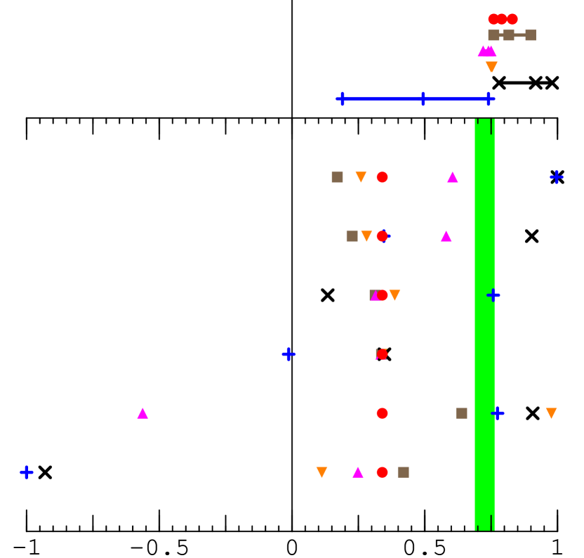
$S_{f}$

Figure 1: Pattern of $S_{f}$ asymmetries for the three scenarios presented in section III.3 with fixed $S_{\pi K_{S}}=0.34$. The symbols represent ${\color[rgb]{1,0,0}\bullet}=\pi$, ${\color[rgb]{0.5,0.4,0.3}\blacksquare}=\eta$, ${\color[rgb]{1,0,1}\blacktriangle}=\eta^{\prime}$, ${\color[rgb]{1,0.5,0}\blacktriangledown}=\phi$, ${\color[rgb]{0,0,0}\boldsymbol{\times}}=\omega$ and ${\color[rgb]{0,0,1}\boldsymbol{+}}=\rho$. The upmost pattern gives the asymmetries in the SM for $\mu=m_{b}/2,m_{b}$ and $2m_{b}$. The other six patterns, from top to bottom, correspond to $(\varepsilon_{z},\theta_{z})=(0.02,0.85)$, $(\varepsilon_{z},\theta_{z})=(0.02,1.79)$, $(\varepsilon_{k},\theta_{k})=(0.02,0.12)$, $(\varepsilon_{k},\theta_{k})=(0.02,2.52)$, $(\varepsilon_{g},\theta_{g})=(1,3.27)$, and $(\varepsilon_{g},\theta_{g})=(1,5.64)$. The vertical bar represents the experimental value for $S_{\psi K_{S}}$.

IV Present Data

At present, the B factories provide constraints on eight relevant CP asymmetries. The data are presented in Table 1. We would like to test various scenarios of new physics by performing a $\chi^{2}$ fit to the data. Since we are mainly interested in demonstrating the potential power of the data to probe new physics in the future, we make several simplifications:

1. We work within the framework defined in section III.B, that is, new physics contributions that depend on only a single complex parameter.

2. Since the measurement of $S_{\psi K_{S}}$ is very accurate, we fix the value of $\sin 2\beta_{\rm eff}$ to its central value, and do not include it as a fit parameter. Furthermore, since experimental data Aubert:2004cp disfavor $\cos 2\beta_{\rm eff}<0$, we allow only positive $\cos 2\beta_{\rm eff}$ values.

We thus calculate, for various scenarios,

$$\chi^{2}(\varepsilon,\theta)\equiv\sum_{f}\left[\frac{X_{f}^{\rm exp}-X_{f}^{\rm QF}(\varepsilon,\theta)}{\sigma_{f}^{\rm exp}}\right]^{2},$$ (28)

where $X_{f}^{\rm exp}$ and $\sigma_{f}^{\rm exp}$ are, respectively, the central value and the one sigma range of the experimental measurements of $S_{f}$ and $C_{f}$ for $f=\pi^{0}K_{S}$, $\eta^{\prime}K_{S}$, $\phi K_{S}$ and $\omega K_{S}$, and $X_{f}^{\rm QF}(\varepsilon,\theta)$ are the (central) theoretical values of $S_{f}$ and $C_{f}$ calculated within the QCD factorization approach for given values of $\varepsilon$ and $\theta$. Only experimental uncertainties are taken into account. Since there are eight observables and two free parameters, $\chi^{2}$ has a six degrees of freedom distribution.

We consider eleven cases. Firstly, we investigate the possibility that the new physics contributes significantly via only a single $O_{i}$, where $i=3,\ldots,10$. (Specific models of new physics do not provide a strong motivation for such scenarios. Yet, this investigation is useful in the two limits discussed in section III.2. If the new physics is dominant and depends on a single weak phase, we can see the universality of its effects [eq. (III.2)]. If the new physics contribution is small, the effects are well approximated by a sum over the shifts from the various operators [eq. (III.2)].) In each case, we perform our analysis for $\varepsilon\leq 5$ and all $\theta\in[0,2\pi]$. Secondly, we investigate the three specific examples presented in section III.3. We do this for $\varepsilon$ within the phenomenologically allowed ranges and for all $\theta$ values.

We use the $\chi^{2}$ fit in two ways. For each case we find the favored regions in the $\varepsilon-\theta$ plane. The results are shown in Figs. 2 and 3. Since the fits to individual operators $O_{3\ldots 10}$ give very similar results for large $\epsilon$, we only show the ones for $O_{4},O_{5}$ and $O_{9}$. Then we test the overall goodness of the fit for each case and learn whether the possibility that the data are accounted for by a new physics contribution to this (set of) operator(s) is disfavored. We draw the following conclusions:

1. For almost all the Wilson coefficients, a very good fit is obtained for a high $\varepsilon$ value, such that eq. (16) holds and the shift is universal [eq. (III.2)]. The reason is that the central values of the three best measured $S_{f}$ asymmetries ($f=\eta^{\prime}K_{S},\phi K_{S},\pi^{0}K_{S}$) show an approximately universal pattern: $\delta S_{f}\sim-0.4$.

2. For operators where eq. (16) gives the best fit, the preferred value of $\theta$ corresponds to $\sin 2(\beta+\theta)\sim 0.4$. Note that a four-fold ambiguity arises, giving $\theta_{i}\sim 55^{o},\ 170^{o},\ 235^{o},\ 350^{o}$, which can be seen in Fig. 2. Had we allowed for $\cos 2\beta_{\rm eff}<0$, there would be eight possible solutions for high $\varepsilon$.

3. For each of the three specific scenarios that we considered, there exists a region in the $\varepsilon-\theta$ plane where a good fit is obtained. Note that within the operator basis we use, in the first two scenarios with modified four-Fermi operators a phase smaller than $\pi$ is preferred, whereas $\pi\leq\theta_{g}<2\pi$ is favored.

4. Naively, the probability that there is no new physics contribution affecting the measured $S_{f}$’s is small. (The SM point, $\varepsilon=0$, lies in the white area.) One has to bear in mind, however, that we used a rather crude approximation, and that there are large uncertainties in our evaluation of the matrix elements. Furthermore, the discrepancy between $S_{\eta^{\prime}K_{S}}^{\rm exp}=0.43\pm 0.11$ and $S_{\eta^{\prime}K_{S}}^{\rm QF}=0.74$ plays a significant role in this result. Note however that the Belle and Babar results for this observable are not quite consistent. Inflating the error according to the PDG prescription would yield $S_{\eta^{\prime}K_{S}}^{\rm exp}=0.43\pm 0.17$ and a better SM fit. (Now the SM point lies in the light grey area.)

$\varepsilon_{4}$

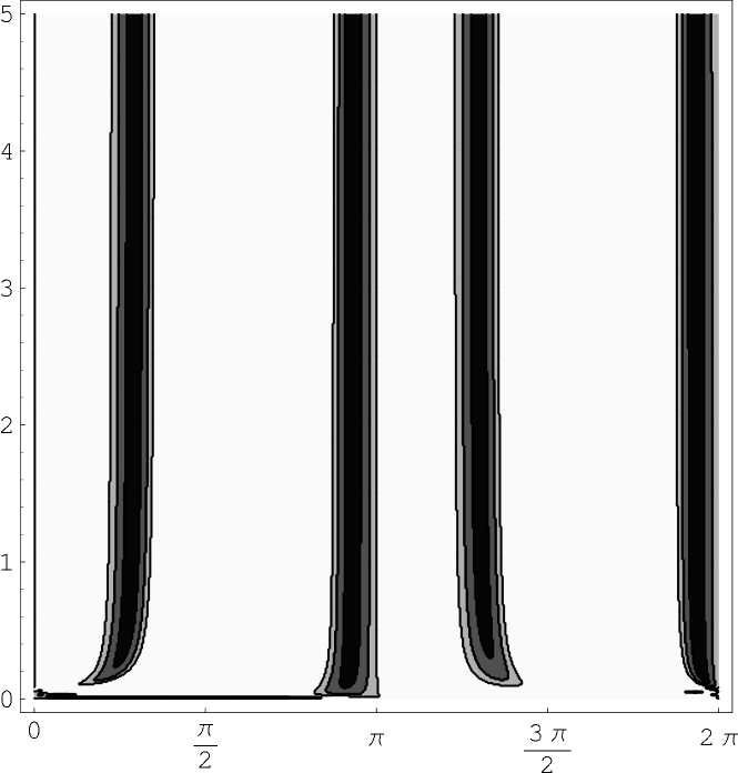
$\theta_{4}$

$\varepsilon_{5}$

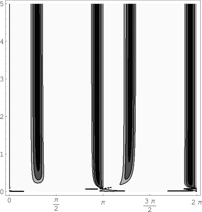
$\theta_{5}$

$\varepsilon_{9}$

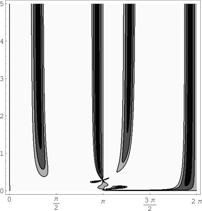
$\theta_{9}$

Figure 2: Allowed region in the $\varepsilon_{i}-\theta_{i}$ plane for new physics in a single operator: (a) $O_{4}$, (b) $O_{5}$ and (c) $O_{9}$. The black, dark grey, and light grey regions correspond to probability higher than 0.32, 0.046, and 0.0027, respectively.

$\varepsilon_{z}$

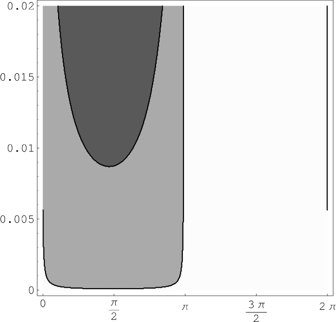
$\theta_{z}$

$\varepsilon_{k}$

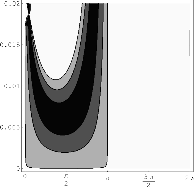
$\theta_{k}$

$\varepsilon_{g}$

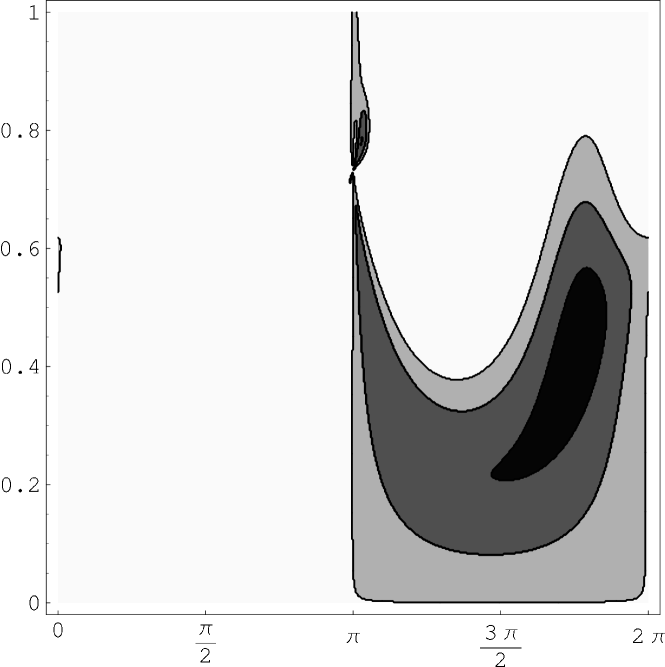
$\theta_{g}$

Figure 3: Allowed regions in the $\varepsilon-\theta$ plane for the three specific scenarios, (a) enhanced $Z$-penguins, (b) KK gluons in RS models, (c) enhanced chromomagnetic operator. The black, dark grey, and light grey regions correspond to probability higher than 0.32, 0.046, and 0.0027, respectively.

V Conclusions

$B$-meson decays that proceed via the quark transition $b\to q\bar{q}s$, for $q=s,d,u$, open a window to new physics because the SM contribution is either loop- or CKM-suppressed. In particular, the CP violating asymmetries $S_{f}$ and $C_{f}$ in these modes may reveal the existence of new sources of CP violation beyond the KM phase.

With new physics, these decays may get significant contributions that depend on a phase that is different from the SM phase. Then, not only will these asymmetries be different from the SM prediction but also, in general, they will differ from each other. The pattern of deviations, $\delta S_{f}=-\eta_{f}S_{f}-S_{\psi K}$ and $C_{f}$, allows us to probe in detail the nature of the new physics that accounts for the effect.

Factorization schemes predict that there is an accidental cancellation between the leading Standard Model contributions to the $\eta K_{S}$, $\omega K_{S}$ and $\rho K_{S}$ modes (see section II). The suppression of the Standard Model amplitudes makes the corresponding CP asymmetries more sensitive to New Physics. At the same time, the sensitivity to hadronic uncertainties is also stronger.

We presented a way to analyze the data in a (new physics) model independent way. In a low energy effective theory, the effects of the new physics are expressed as modifications of Wilson coefficients in the $\Delta B=1$ effective Hamiltonian. The data can be used to find which Wilson coefficients are modified and by what (complex) factor.

The analysis is simplified when the modification of the Wilson coefficients depends on a single complex parameter, as is often the case in specific models. We gave analytic expressions for the modifications in some interesting limits. In particular, for $C_{3,\ldots,10,8g}$, when the new physics dominates, a universal shift of the asymmetries arises [see eq. (III.2)]. If the new physics contribution is small, then the deviations (for $f=\eta^{\prime}K_{S},\phi K_{S},\pi^{0}K_{S},\eta K_{S}$) have a pattern that depends in a simple way on the $b_{f}^{c}$-parameters [see eq. (III.2)].

We applied this method to present data, using lowest order QCD factorization to calculate the hadronic matrix elements. We find that, since the best three measured $S_{f}$’s have similar central values ($\sim 0.4$) which are, however, different from $S_{\psi K}$, and all measured $C_{f}$’s are consistent with zero, a good fit can be achieved for almost all operators if they are enhanced by the new physics to a level where they dominate over the SM contribution. In three specific scenarios that we considered, such new physics dominance cannot be realized in Nature because of phenomenological constraints. Still, a good fit can be obtained for each of these scenarios.

Our analysis can be improved in several ways. In particular, the calculation should go beyond the leading log approximation and incorporate power corrections. The combination of improved calculations, more accurate measurements and additional modes explored experimentally, is likely to make the pattern of deviations from the SM (or their absence) a powerful probe of flavor and CP violating new physics.

- (1) D. Kirkby and and Y. Nir, review of ‘CP violation in meson decays,’ in S. Eidelman et al. [Particle Data Group Collaboration], Phys. Lett. B 592, 1 (2004).
- (2) Y. Grossman and M. P. Worah, Phys. Lett. B 395, 241 (1997) [arXiv:hep-ph/9612269]; R. Fleischer, Int. J. Mod. Phys. A 12, 2459 (1997) [arXiv:hep-ph/9612446]; M. Ciuchini, E. Franco, G. Martinelli, A. Masiero and L. Silvestrini, Phys. Rev. Lett. 79, 978 (1997) [arXiv:hep-ph/9704274]; D. London and A. Soni, Phys. Lett. B 407, 61 (1997) [arXiv:hep-ph/9704277].
- (3) M. Beneke, G. Buchalla, M. Neubert and C. T. Sachrajda, Nucl. Phys. B 591, 313 (2000) [arXiv:hep-ph/0006124]; Nucl. Phys. B 606, 245 (2001) [arXiv:hep-ph/0104110].
- (4) A. Ali, G. Kramer and C. D. Lü, Phys. Rev. D 58, 094009 (1998) [arXiv:hep-ph/9804363].
- (5) M. Beneke and M. Neubert, Nucl. Phys. B 651, 225 (2003) [arXiv:hep-ph/0210085].
- (6) K. Abe et al. [Belle Collaboration], arXiv:hep-ex/0408111.
- (7) B. Aubert et al. [BABAR Collaboration], arXiv:hep-ex/0408127.
- (8) B. Aubert et al. [BABAR Collaboration], arXiv:hep-ex/0502019.
- (9) K. Abe et al. [Belle Collaboration], arXiv:hep-ex/0409049; K. F. Chen [Belle Collaboration], arXiv:hep-ex/0504023.
- (10) B. Aubert et al. [the BaBar Collaboration], arXiv:hep-ex/0502017.
- (11) B. Aubert et al. [BABAR Collaboration], arXiv:hep-ex/0503011.
- (12) B. Aubert et al. [BABAR Collaboration], arXiv:hep-ex/0503018.
- (13) G. Buchalla, A. J. Buras and M. E. Lautenbacher, Rev. Mod. Phys. 68, 1125 (1996) [arXiv:hep-ph/9512380].
- (14) K. G. Chetyrkin, M. Misiak and M. Münz, Nucl. Phys. B 520, 279 (1998) [arXiv:hep-ph/9711280];
- (15) K. Baranowski and M. Misiak, Phys. Lett. B 483, 410 (2000) [arXiv:hep-ph/9907427].
- (16) J. Charles et al. [CKMfitter Group], arXiv:hep-ph/0406184; M. Bona et al. [UTfit Collaboration], arXiv:hep-ph/0501199.
- (17) H. J. Lipkin, Phys. Rev. Lett. 46, 1307 (1981).
- (18) Talk given by Martin Beneke at the CKM2005 Workshop on the Unitarity Triangle, San Diego, March 15, 2005, http://ckm2005.ucsd.edu; arXiv:hep-ph/0505075.
- (19) D. Atwood and G. Hiller, arXiv:hep-ph/0307251.
- (20) G. Burdman, Phys. Lett. B 590, 86 (2004) [arXiv:hep-ph/0310144].
- (21) K. Agashe, G. Perez and A. Soni, Phys. Rev. Lett. 93, 201804 (2004) [arXiv:hep-ph/0406101]; Phys. Rev. D 71, 016002 (2005) [arXiv:hep-ph/0408134].
- (22) T. E. Coan et al. [CLEO Collaboration], Phys. Rev. Lett. 80, 1150 (1998) [arXiv:hep-ex/9710028].
- (23) A. Kagan, arXiv:hep-ph/9806266.
- (24) B. Aubert et al. [BABAR Collaboration], arXiv:hep-ex/0411016.