Higgs Sector of the Left-Right Model with Explicit CP Violation

Abstract

We explore the Higgs sector of the Minimal Left-Right (LR) Model based on the gauge group $SU(2)_{L}\times SU(2)_{R}\times U(1)_{B-L}$ with explicit CP violation in the Higgs potential. Since flavour-changing neutral current experiments and the small scale of neutrino masses both place stringent constraints on the Higgs potential, we seek to determine whether minima of the Higgs potential exist that are consistent with current experimental bounds. We focus on the case in which the right-handed symmetry-breaking scale is only “moderately” large, of order 15-50 TeV. Unlike the case in which the Higgs potential is CP-invariant, the CP noninvariant case does yield viable scenarios, although these require a small amount of fine-tuning. We consider a LR model supplemented by an additional $U(1)$ horizontal symmetry, which results in a Higgs sector consistent with current experimental constraints and a realistic spectrum of neutrino masses.

I Introduction

Left-Right (LR) models have long provided attractive extensions to the well-tested Standard Model (SM) of particle physics patisalam1974 ; mohapatrapati ; mohapatrapati1975 ; senjanovic ; mohapatrapaige ; senjanovic1979 ; duka . A typical LR model is constructed by enlarging the SM gauge group $SU(2)_{L}\times U(1)_{Y}$ to the group $SU(2)_{L}\times SU(2)_{R}\times U(1)_{B-L}$ and thus contains an extra set of $W$ and $Z$ gauge bosons compared to the Standard Model, as well as an extended Higgs structure. Minimal versions of the left-right model usually contain one bidoublet Higgs boson, $\phi$, as well as left- and right-handed triplet Higgs bosons, $\Delta_{L,R}$, although other constructions are also possible (see for example Ref. Ma03 ).

There are several reasons for the appeal of LR models. Among these is the fact that, unlike in the SM, the $U(1)$ symmetry of the theory has a physical interpretation in terms of baryon and lepton number. Also, the observed parity-odd nature of the low-energy weak interactions is seen to be the result of a spontaneously broken symmetry in the LR Model. Furthermore, it has been pointed out that, since parity is an exact symmetry of the theory at high energies, the strong CP problem has a natural solution in the context of LR models MoSen ; BegTsao . In addition, the choice of a Higgs triplet to break left-right symmetry at a high energy scale leads naturally to a seesaw relation to explain the smallness of neutrino masses mohapatra1980 ; Mohapatra:1980yp . Finally, the extended Higgs sector of the theory gives the possibility, at least in principle, of breaking CP spontaneously.

Many authors have focused on the possibility of spontaneous CP violation in LR models, both in minimal versions as well as in extended versions containing more complicated Higgs sectors branco ; basecq ; gunion ; deshpande ; gluza ; bgnr . The results in minimal versions of the LR Model have by and large been somewhat negative regarding the possibility of generating spontaneous CP violation, while investigations of more complicated models have had more encouraging results. A further complication in the case of the minimal model concerns the presence of neutral Higgs bosons having flavour-violating couplings to quarks (Flavour Changing Neutral Higgs (FCNH) bosons). Recently, Barenboim et al studied the decoupling limit of the minimal CP-invariant Higgs potential in the LR model bgnr . They found that non-negligible CP violation in the vacuum state is generally accompanied by weak-scale non-standard Higgs bosons, which are ruled out phenomenologically. For CP-conserving vacuum states they found that it was possible to produce an acceptable physical Higgs spectrum, but only at the cost of extreme fine-tuning.

Another well-known complication in the Higgs sector of LR models concerns the vacuum expectation value (VEV) of the neutral component of the left-handed Higgs triplet, $\langle\delta_{L}^{0}\rangle\sim v_{L}e^{i\theta_{L}}$. Assuming that all dimensionless coefficients in the Higgs potential are of order unity, $v_{L}$ is related to its right-handed counterpart $v_{R}$ through a seesaw relation, $v_{L}\sim k^{2}/v_{R}$, where $k$ is a dimensionful quantity of order of the weak scale. The complication resides in the fact that, in general, the left-handed neutrino mass matrix contains a term that is proportional to $v_{L}$. Barring extreme fine-tunings, this term in the mass matrix forces $v_{L}$ to be of order a few eV or less, thereby forcing the right-handed scale, $v_{R}$, to be extremely large. To allow for the possibility of an observable right-handed scale, many authors assume that $v_{L}=0$, a scenario that can be arranged by disallowing certain terms from the Higgs potential. The offending terms in the Higgs potential have the form $\mbox{Tr}\!\left(\phi\Delta_{R}\phi^{\dagger}\Delta_{L}^{\dagger}\right)$ and may be forbidden, for example, by imposing a symmetry under the discrete operation $\Delta_{L}\to\Delta_{L}$ and $\Delta_{R}\to-\Delta_{R}$. Unfortunately, invariance under this symmetry also disallows the Majorana Yukawa couplings that give rise to the seesaw relation for neutrino masses deshpande . Another approach is simply to assume that the theory is embedded in a grand unified scheme that somehow disallows the troublesome terms from the Higgs potential but still allows the desired Majorana Yukawa terms. This of course does not solve this problem within the LR model framework.

In this paper we analyze the Higgs sector of the minimal LR Model in the case that CP is not a manifest symmetry of the unbroken theory, a scenario that has not received much attention. In the most general case, the introduction of explicit CP violation corresponds to the introduction of only one complex coefficient into the Higgs potential, i.e. only one extra degree of freedom. As we shall see below, the phase associated with this complex coefficient significantly alters the dynamics of the Higgs sector, and we find that the presence of CP violation in the vacuum state no longer precludes the existence of an acceptable Higgs spectrum.

In our calculation, in order to suppress $v_{L}$ to phenomenologically acceptable levels, we further assume the presence of an extra horizontal symmetry that is broken by a small parameter $\epsilon_{H}$ froggatt ; nir1993 ; khasanov . An appropriate choice of charge assignments under this symmetry suppresses certain coefficients in the Higgs potential and brings $v_{L}$ down to the eV scale for moderately light right-handed scales ($v_{R}\sim 15$ TeV, say). The model still does contain a certain amount of fine-tuning. In particular, one dimensionless coefficient in the Higgs potential needs to be “unnaturally” small (of order $k^{2}/v_{R}^{2}$). Since we restrict our attention to right-handed scales that are only “moderately” large, this fine-tuning is not as unnatural as it might be in general.

Our paper is organized as follows. In Sec. II we describe the model and perform the minimization of the Higgs potential to obtain relations among the various Higgs VEVs. Section III contains several approximate expressions for the Higgs boson masses. Section IV contains our numerical results and in Sec. V we offer some concluding remarks. The Appendix describes the derivations of the approximate expressions for the Higgs boson masses.

II The Model

II.1 Minimization of the Higgs Potential

We consider a LR model with a single bidoublet field $\phi\sim(2,\overline{2},0)$ and triplet fields $\Delta_{L}\sim(3,1,2)$ and $\Delta_{R}\sim(1,3,2)$. Under $SU(2)_{L}\times SU(2)_{R}$ the fermion fields in the theory transform as $\Psi_{L,R}\to U_{L,R}\Psi_{L,R}$ and the Higgs fields transform as $\phi\to U_{L}\phi U_{R}^{\dagger}$ and $\Delta_{L,R}\to U_{L,R}\Delta_{L,R}U_{L,R}^{\dagger}$. We also define the field $\tilde{\phi}=\tau_{2}\phi^{*}\tau_{2}$, which transforms in the same way as $\phi$. The full Lagrangian of the theory (denoted below as LR Model) is invariant under the LR symmetry operation

$$\Psi_{L}\leftrightarrow\Psi_{R},~{}~{}~{}~{}\phi\leftrightarrow\phi^{\dagger},~{}~{}~{}~{}\tilde{\phi}\leftrightarrow\tilde{\phi}^{\dagger},~{}~{}~{}~{}\Delta_{L}\leftrightarrow\Delta_{R}.$$ (1)

The most general LR symmetric Higgs potential that can be constructed from $\phi$, $\tilde{\phi}$, $\Delta_{L}$ and $\Delta_{R}$ may be parameterized as follows deshpande ,

$$V = -\mu_{1}^{2}\left[\mbox{Tr}\!\left(\phi^{\dagger}\phi\right)\right]-\mu_{2}^{2}\left[\mbox{Tr}\!\left(\tilde{\phi}\phi^{\dagger}\right)+\mbox{Tr}\!\left(\tilde{\phi}^{\dagger}\phi\right)\right]-\mu_{3}^{2}\left[\mbox{Tr}\!\left(\Delta_{L}\Delta_{L}^{\dagger}\right)+\mbox{Tr}\!\left(\Delta_{R}\Delta_{R}^{\dagger}\right)\right]$$ (2)

$$+\lambda_{1}\left[\mbox{Tr}\!\left(\phi\phi^{\dagger}\right)\right]^{2}+\lambda_{2}\left\{\left[\mbox{Tr}\!\left(\tilde{\phi}\phi^{\dagger}\right)\right]^{2}+\left[\mbox{Tr}\!\left(\tilde{\phi}^{\dagger}\phi\right)\right]^{2}\right\}+\lambda_{3}\left[\mbox{Tr}\!\left(\tilde{\phi}\phi^{\dagger}\right)\mbox{Tr}\!\left(\tilde{\phi}^{\dagger}\phi\right)\right]$$

$$+\lambda_{4}\left\{\mbox{Tr}\!\left(\phi\phi^{\dagger}\right)\left[\mbox{Tr}\!\left(\tilde{\phi}\phi^{\dagger}\right)+\mbox{Tr}\!\left(\tilde{\phi}^{\dagger}\phi\right)\right]\right\}+\rho_{1}\left\{\left[\mbox{Tr}\!\left(\Delta_{L}\Delta_{L}^{\dagger}\right)\right]^{2}+\left[\mbox{Tr}\!\left(\Delta_{R}\Delta_{R}^{\dagger}\right)\right]^{2}\right\}$$

$$+\rho_{2}\left[\mbox{Tr}\!\left(\Delta_{L}\Delta_{L}\right)\mbox{Tr}\!\left(\Delta_{L}^{\dagger}\Delta_{L}^{\dagger}\right)+\mbox{Tr}\!\left(\Delta_{R}\Delta_{R}\right)\mbox{Tr}\!\left(\Delta_{R}^{\dagger}\Delta_{R}^{\dagger}\right)\right]+\rho_{3}\left[\mbox{Tr}\!\left(\Delta_{L}\Delta_{L}^{\dagger}\right)\mbox{Tr}\!\left(\Delta_{R}\Delta_{R}^{\dagger}\right)\right]$$

$$+\rho_{4}\left[\mbox{Tr}\!\left(\Delta_{L}\Delta_{L}\right)\mbox{Tr}\!\left(\Delta_{R}^{\dagger}\Delta_{R}^{\dagger}\right)+\mbox{Tr}\!\left(\Delta_{L}^{\dagger}\Delta_{L}^{\dagger}\right)\mbox{Tr}\!\left(\Delta_{R}\Delta_{R}\right)\right]$$

$$+\alpha_{1}\left\{\mbox{Tr}\!\left(\phi\phi^{\dagger}\right)\left[\mbox{Tr}\!\left(\Delta_{L}\Delta_{L}^{\dagger}\right)+\mbox{Tr}\!\left(\Delta_{R}\Delta_{R}^{\dagger}\right)\right]\right\}$$

$$+\alpha_{2}\left\{e^{i\delta_{2}}\left[\mbox{Tr}\!\left(\phi\tilde{\phi}^{\dagger}\right)\mbox{Tr}\!\left(\Delta_{R}\Delta_{R}^{\dagger}\right)+\mbox{Tr}\!\left(\phi^{\dagger}\tilde{\phi}\right)\mbox{Tr}\!\left(\Delta_{L}\Delta_{L}^{\dagger}\right)\right]+\mbox{h.c.}\right\}$$

$$+\alpha_{3}\left[\mbox{Tr}\!\left(\phi\phi^{\dagger}\Delta_{L}\Delta_{L}^{\dagger}\right)+\mbox{Tr}\!\left(\phi^{\dagger}\phi\Delta_{R}\Delta_{R}^{\dagger}\right)\right]+\beta_{1}\left[\mbox{Tr}\!\left(\phi\Delta_{R}\phi^{\dagger}\Delta_{L}^{\dagger}\right)+\mbox{Tr}\!\left(\phi^{\dagger}\Delta_{L}\phi\Delta_{R}^{\dagger}\right)\right]$$

$$+\beta_{2}\left[\mbox{Tr}\!\left(\tilde{\phi}\Delta_{R}\phi^{\dagger}\Delta_{L}^{\dagger}\right)+\mbox{Tr}\!\left(\tilde{\phi}^{\dagger}\Delta_{L}\phi\Delta_{R}^{\dagger}\right)\right]+\beta_{3}\left[\mbox{Tr}\!\left(\phi\Delta_{R}\tilde{\phi}^{\dagger}\Delta_{L}^{\dagger}\right)+\mbox{Tr}\!\left(\phi^{\dagger}\Delta_{L}\tilde{\phi}\Delta_{R}^{\dagger}\right)\right]\;.$$

All of the coefficients in the above expression are real, with the exception of the term proportional to $\alpha_{2}$, which has a phase $\delta_{2}$. ( The coefficient $\alpha_{2}$ itself will be taken to be real and non-negative in this work.) Papers on this subject have nearly universally set $\sin\delta_{2}$ to zero. As pointed out in Ref. bgnr , however, setting $\sin\delta_{2}$ to zero effectively means the vacuum state will not break CP. In contrast to this, we will see that it is quite natural to have large CP-violating phases in the Higgs VEVs in the case $\sin\delta_{2}\neq 0$.

We adopt the following notation for the various components of $\phi$, $\Delta_{L}$ and $\Delta_{R}$,

$$\phi=\left(\begin{array}[]{cc}\phi_{1}^{0}&\phi_{1}^{+}\\ \phi_{2}^{-}&\phi_{2}^{0}\\ \end{array}\right),~{}~{}~{}\Delta_{L,R}=\left(\begin{array}[]{cc}\delta_{L,R}^{+}/\sqrt{2}&\delta_{L,R}^{++}\\ \delta_{L,R}^{0}&-\delta_{L,R}^{+}/\sqrt{2}\\ \end{array}\right).$$ (7)

The lepton Yukawa couplings that are consistent with the gauge and parity symmetries discussed above are

$$-{\mathcal{L}}_{\textrm{\scriptsize Yukawa}}=\overline{\psi}_{iL}^{\prime}\left(G_{ij}\phi+H_{ij}\widetilde{\phi}\right)\psi_{jR}^{\prime}+\frac{i}{2}F_{ij}\left(\psi^{\prime T}_{iL}C\tau_{2}\Delta_{L}\psi^{\prime}_{jL}+\psi^{\prime T}_{iR}C\tau_{2}\Delta_{R}\psi^{\prime}_{jR}\right)+\textrm{h.c.}\;,$$ (8)

where $F$, $G$ and $H$ are $3\times 3$ Yukawa matrices, $C=i\gamma^{2}\gamma^{0}$ is the charge conjugation matrix and primes denote gauge eigenstates. Upon spontaneous symmetry breaking, the neutral components of the Higgs boson fields obtain VEVs,

$$\langle\phi\rangle=\left(\begin{array}[]{cc}k_{1}/\sqrt{2}&0\\ 0&k_{2}e^{i\alpha}/\sqrt{2}\\ \end{array}\right),~{}~{}~{}\langle\Delta_{L}\rangle=\left(\begin{array}[]{cc}0&0\\ v_{L}e^{i\theta_{L}}/\sqrt{2}&0\\ \end{array}\right),~{}~{}~{}\langle\Delta_{R}\rangle=\left(\begin{array}[]{cc}0&0\\ v_{R}/\sqrt{2}&0\\ \end{array}\right),$$ (15)

where $k_{1}$, $k_{2}$, $v_{L}$ and $v_{R}$ all refer to the magnitudes of the respective quantities. Phenomenological considerations lead to the conclusion that $v_{L}\ll k_{1},k_{2}\ll v_{R}$. Furthermore, $k_{1}$ and $k_{2}$ are at the weak scale, $k_{1}^{2}+k_{2}^{2}\simeq(246$ GeV$)^{2}$. Gauge rotations have been used in the above expressions to eliminate possible phases in the $k_{1}$ and $v_{R}$ terms deshpande . The four complex neutral fields may then be expanded in terms of eight real fields as follows,

$$\phi_{1}^{0} = (\phi_{1}^{0r}+i\phi_{1}^{0i}+k_{1})/\sqrt{2},$$ (16)

$$\phi_{2}^{0} = (\phi_{2}^{0r}+i\phi_{2}^{0i}+k_{2})e^{i\alpha}/\sqrt{2},$$ (17)

$$\delta_{L}^{0} = (\delta_{L}^{0r}+i\delta_{L}^{0i}+v_{L})e^{i\theta_{L}}/\sqrt{2},$$ (18)

$$\delta_{R}^{0} = (\delta_{R}^{0r}+i\delta_{R}^{0i}+v_{R})/\sqrt{2}.$$ (19)

Minimizing the potential in Eq. (2) with respect to $\phi_{1}^{0r}$, $\phi_{2}^{0r}$, $\phi_{2}^{0i}$, $\delta_{R}^{0r}$, $\delta_{L}^{0r}$ and $\delta_{L}^{0i}$ leads to six equations that need to be satisfied by the coefficients of the potential. By manipulating these expressions we obtain expressions for the $\mu_{i}^{2}$,

$$\frac{\mu_{1}^{2}}{v_{R}^{2}} = \frac{\alpha_{1}}{2}\left(1+\frac{v_{L}^{2}}{v_{R}^{2}}\right)-\frac{\alpha_{3}\xi^{2}}{2(1-\xi^{2})}\left(1+\frac{v_{L}^{2}}{v_{R}^{2}}\right)+\left[\lambda_{1}\left(1+\xi^{2}\right)+2\lambda_{4}\xi\cos\alpha\right]\epsilon^{2}$$ (20)

$$+\left[\beta_{2}\cos\theta_{L}-\beta_{3}\xi^{2}\cos(\theta_{L}-2\alpha)\right]\frac{v_{L}/v_{R}}{1-\xi^{2}}\;,$$

$$\frac{\mu_{2}^{2}}{v_{R}^{2}} = \frac{\alpha_{2}}{2\cos\alpha}\left[\cos(\alpha+\delta_{2})+\cos(\alpha-\delta_{2})\frac{v_{L}^{2}}{v_{R}^{2}}\right]+\frac{\alpha_{3}\xi}{4(1-\xi^{2})\cos\alpha}\left(1+\frac{v_{L}^{2}}{v_{R}^{2}}\right)$$ (21)

$$+\left[2\lambda_{2}\xi\cos(2\alpha)+\lambda_{3}\xi+\frac{1}{2}\lambda_{4}\left(1+\xi^{2}\right)\cos\alpha\right]\frac{\epsilon^{2}}{\cos\alpha}$$

$$+\left[\beta_{1}(1-\xi^{2})\cos(\theta_{L}-\alpha)-2\beta_{2}\xi\cos\theta_{L}+2\beta_{3}\xi\cos(\theta_{L}-2\alpha)\right]\frac{v_{L}/v_{R}}{4(1-\xi^{2})\cos\alpha}\;,$$

$$\frac{\mu_{3}^{2}}{v_{R}^{2}} = \rho_{1}\left(1+\frac{v_{L}^{2}}{v_{R}^{2}}\right)+\frac{1}{2}\left[\alpha_{1}\left(1+\xi^{2}\right)+\alpha_{3}\xi^{2}\right]\epsilon^{2}$$ (22)

$$+2\alpha_{2}\left[\cos(\alpha+\delta_{2})-\cos(\alpha-\delta_{2})\frac{v_{L}^{2}}{v_{R}^{2}}\right]\frac{\xi\epsilon^{2}}{1-v_{L}^{2}/v_{R}^{2}}\;,$$

where we have defined $\xi\equiv k_{2}/k_{1}$ and $\epsilon\equiv k_{1}/v_{R}$. Both $\xi$ and $\epsilon$ are small quantities in our analysis. We also obtain three other equalities that must be satisfied,

$$\left[(2\rho_{1}-\rho_{3})-\frac{8\alpha_{2}\xi\epsilon^{2}\sin\alpha\sin\delta_{2}}{1-v_{L}^{2}/v_{R}^{2}}\right]\frac{v_{L}}{v_{R}}$$ (23)

$$= \left[\beta_{1}\xi\cos(\theta_{L}-\alpha)+\beta_{2}\cos\theta_{L}+\beta_{3}\xi^{2}\cos(\theta_{L}-2\alpha)\right]\epsilon^{2}\;,$$

$$0 = \beta_{1}\xi\sin(\theta_{L}-\alpha)+\beta_{2}\sin\theta_{L}+\beta_{3}\xi^{2}\sin(\theta_{L}-2\alpha)\;,$$ (25)

$$2\alpha_{2}\left(1-\xi^{2}\right)\left(1-v_{L}^{2}/v_{R}^{2}\right)\sin\delta_{2}$$

$$= \left\{2\xi\sin(\theta_{L}-\alpha)(\beta_{2}+\beta_{3})+\left[\sin\theta_{L}+\xi^{2}\sin(\theta_{L}-2\alpha)\right]\beta_{1}\right\}\frac{v_{L}}{v_{R}}$$

$$+\xi\sin\alpha\left[\alpha_{3}\left(1+v_{L}^{2}/v_{R}^{2}\right)+(4\lambda_{3}-8\lambda_{2})\left(1-\xi^{2}\right)\epsilon^{2}\right]\;.$$

Taking $\delta_{2}\to 0$ in Eqs. (23)-(25) gives Eqs. (A5)-(A7) in Ref. deshpande . Equation (23) yields the well-known seesaw relation for $v_{L}$, $v_{L}\sim(\mbox{some couplings})\times\epsilon^{2}v_{R}$. Interestingly, $\rho_{2}$ and $\rho_{4}$ do not appear in the above expressions and are thus not constrained by the first-derivative conditions. (The first of these does, however, appear in an approximate expression for one of the Higgs boson masses and is thus constrained through a second-derivative condition.)

A very important feature of the above equations is that the left-hand side of Eq. (25) is generically non-zero. This gives us considerably more freedom when solving the minimization conditions compared to the situation considered throughout much of Ref. bgnr (in which it was mostly assumed that $\sin\delta_{2}=0$). In particular, in our case we can easily obtain $\alpha_{3}={\cal O}(1)$ instead of ${\cal O}(\epsilon^{2})$. This observation is crucial, since the neutral Higgs bosons with flavour non-diagonal couplings to quarks have masses $\sim\sqrt{\alpha_{3}v_{R}^{2}/2}$ (see Eq. (43) below). If $\alpha_{3}={\cal O}(1)$, these FCNH bosons attain masses at the scale $v_{R}$ and are phenomenologically viable. If, however, $\alpha_{3}$ is of order $\epsilon^{2}$, then the FCNH bosons have masses at the weak scale, a scenario that presents considerable phenomenological problems. Let us examine this argument a bit more quantitatively. Suppose for the moment that $\sin\delta_{2}=0$ and $v_{L}/v_{R}\ll 1$. Suppose furthermore that $\sin\alpha\neq 0$, so that the vacuum state breaks CP. In order to satisfy Eq. (25) in this case, one must have $\alpha_{3}\simeq(8\lambda_{2}-4\lambda_{3})(1-\xi^{2})\epsilon^{2}$; i.e., unless $\lambda_{2}$ is very large, $\alpha_{3}$ must be of order $\epsilon^{2}$, leading to phenomenological difficulties. If $\sin\delta_{2}\neq 0$, however, things are quite different. In this case Eq. (25) becomes

$$2\alpha_{2}\sin\delta_{2}\simeq\alpha_{3}\xi\sin\alpha\;$$ (26)

(where we have assumed that $v_{L}/v_{R}$ is negligibly small and that the various Higgs coefficients are not anomalously large). It is possible to satisfy this expression with $\alpha_{3}={\cal O}(1)$. In particular, we can use the above expression to determine the phase of $\langle\phi_{2}^{0}\rangle$,

$$\alpha\simeq\sin^{-1}\left(\frac{2\alpha_{2}\sin\delta_{2}}{\alpha_{3}\xi}\right).$$ (27)

With the choice we make below for the charges under the approximate horizontal symmetry, we have $\alpha_{3}\sim{\cal O}(1)$ and $\alpha_{2}\sim{\cal O}(\xi)$. In this case $\alpha$ is of order unity if $\delta_{2}$ is. To summarize, if $\sin\delta_{2}$ is non-zero, one can in fact have a vacuum state that violates CP while simultaneously evading the FCNH problem. This possibility was noted in Ref. bgnr , but was not explored in detail.

II.2 A Broken Horizontal Symmetry

Let us return to the seesaw relation for the VEVs derived from Eq. (23) and noted above. If all the coefficients in the Higgs potential are of order unity one has $v_{L}\sim(\mbox{some couplings})\times\epsilon^{2}v_{R}$ (note that $\epsilon^{2}v_{R}=k_{1}^{2}/v_{R})$. If $k_{1}$ is of order the weak scale and $v_{R}$ is of order 10’s of TeV, then $v_{L}$ is of order a few GeV. Such a value for $v_{L}$ is extraordinarily large from the point of view of neutrino physics, an observation that can be understood by examining the $3\times 3$ mass matrix for the light, mostly left-handed neutrinos. This mass matrix is given by the following approximate expression,

$$M_{\nu}\simeq M_{LL}^{\dagger}-M_{LR}M_{RR}^{-1}M_{LR}^{T},$$ (28)

where

$$M_{LR}=(Gk_{1}+Hk_{2}e^{-i\alpha})/\sqrt{2},~{}~{}~{}M_{LL}=Fv_{L}e^{i\theta_{L}}/\sqrt{2},~{}~{}~{}M_{RR}=Fv_{R}/\sqrt{2},$$ (29)

with $F$, $G$ and $H$ being $3\times 3$ Yukawa matrices (see Eq. (8)). Phenomenologically, the elements of $M_{\nu}$ must be at the eV scale (or smaller). The second term in Eq. (28) is the usual “seesaw” term – it scales roughly as $k_{1}^{2}/v_{R}$, thereby suppressing the neutrinos’ masses. If $v_{R}$ is only “moderately” large (of order 10’s of TeV), the Yukawa matrices $G$ and $H$ need to be suppressed in order that the elements in this term are at the eV scale. The first term in Eq. (28) also benefits from a seesaw relation in that it is proportional to $v_{L}\sim k_{1}^{2}/v_{R}$. The seesaw suppression is not enough if $v_{R}={\cal O}(10~{}\mbox{TeV})$, however, since then $v_{L}$ is of order a few GeV (as noted above). To solve the problem, one could suppress $M_{LL}$ by forcing the elements of $F$ to be very tiny (of order $10^{-10}$, say), but then the right-handed Majorana mass terms ($M_{RR}$) would also become very small (of order keV for $v_{R}$ of order 10’s of TeV). This would render the seesaw mechanism for neutrino masses inoperative (in fact, Eq. (28) would become invalid) and would generically yield GeV-scale neutrinos. To remedy the situation one needs to force the coefficients $\beta_{i}$ in Eq. (23) to be very small or zero, thereby forcing $v_{L}$ to be very small or zero. The $\beta_{i}$ can be made to disappear via an exact symmetry, but, as shown in Ref. deshpande , the disappearance of the $\beta_{i}$ comes at the expense of Majorana or Dirac mass terms in this case.

A simple approach that suppresses the $\beta_{i}$ without eliminating them completely is to adopt an approximate horizontal $U(1)$ symmetry that is broken by a small parameter $\epsilon_{H}$ froggatt ; nir1993 ; khasanov . In this approach, each of the fields in the theory is assigned a charge under the symmetry, and terms in the Lagrangian that are not singlets under this symmetry become suppressed by $\epsilon_{H}^{n}$, where $n$ is some combination of the charges of the fields involved. We adopt the charge assignments khasanov

$$Q(\Delta_{L}) = -Q(\Delta_{R})=-8,$$ (30)

$$Q(\phi) = -2,$$ (31)

with the result that the dimensionless coefficients in the Higgs potential scale as follows

$$\begin{array}[]{rcl}\alpha_{1},\alpha_{3}\sim{\cal O}(1),~{}~{}~{}\alpha_{2}&\sim&{\cal O}(\epsilon_{H}^{4})\sim{\cal O}(\xi)\\ \beta_{1}\sim{\cal O}(\epsilon_{H}^{16}),~{}~{}~{}\beta_{2}&\sim&{\cal O}(\epsilon_{H}^{20}),~{}~{}~{}\beta_{3}\sim{\cal O}(\epsilon_{H}^{12})\\ \lambda_{1},\lambda_{3}\sim{\cal O}(1),~{}~{}~{}\lambda_{2}\sim{\cal O}(\epsilon_{H}^{8})&\sim&{\cal O}(\xi^{2}),~{}~{}~{}\lambda_{4}\sim{\cal O}(\epsilon_{H}^{4})\sim{\cal O}(\xi)\\ \rho_{1},\rho_{2},\rho_{3}\sim{\cal O}(1),&&\rho_{4}\sim{\cal O}(\epsilon_{H}^{32})\;.\\ \end{array}$$ (36)

In the numerical work below we set $\epsilon_{H}=0.3$ and $\xi=k_{2}/k_{1}=3/181\simeq 0.017$ kiersLR , so that $\epsilon_{H}^{4}\sim\xi$, as noted in the expressions above. Furthermore, for a moderate right-handed scale (of order 15 TeV), $\epsilon=k_{1}/v_{R}\sim(246~{}\mbox{GeV}/(1.5\times 10^{4}~{}\mbox{GeV})\sim 0.016$, so that $\epsilon\sim\xi$. (Of course, for very large right-handed scales $\epsilon$ becomes much less than $\xi$.) The $\beta_{i}$ are particularly suppressed in this scheme, with the result that the VEV seesaw relation now becomes

$$v_{L}\sim\epsilon_{H}^{20}\epsilon^{2}v_{R}.$$ (37)

Taking $v_{R}={\cal O}(15$ TeV$)$, we have $v_{L}\sim 0.1$ eV, which is phenomenologically acceptable.

II.3 Approximate Expressions for the Minimization Equations

It is useful to consider approximate versions of the six minimization equations (Eqs. (20)-(25)), which can be obtained by expanding in the small parameters $\xi$, $\epsilon$ and $v_{L}/v_{R}$ (as well as taking into account the charge assignments for the various Higgs potential coefficients). Of these, we consider $\epsilon$ and $\xi$ to be of approximately the same order (approximately $0.017$), while $v_{L}/v_{R}$ is miniscule (of order $10^{-14}$). We also bear in mind the scaling of the various coefficients in (36), recalling that $\epsilon_{H}^{4}\sim\xi$. An approximate (and slightly rearranged) version of Eq. (25) has already been given above in Eq. (26). (The corrections to this expression are of order $\epsilon^{2}\xi$ and $\xi^{3}$.) Furthermore, Eq. (25) does not need to be expanded at all, since each of the three terms is of approximately the same order. From the other four equations we obtain the following expressions,

$$\frac{\mu_{1}^{2}}{v_{R}^{2}} = \frac{\alpha_{1}}{2}-\frac{1}{2}\alpha_{3}\xi^{2}+\lambda_{1}\epsilon^{2}+{\cal O}(\xi^{4},\xi^{2}\epsilon^{2})\;,$$ (38)

$$\frac{\mu_{2}^{2}}{v_{R}^{2}} = \frac{\alpha_{2}}{2}\frac{\cos(\alpha+\delta_{2})}{\cos\alpha}+\frac{\alpha_{3}\xi}{4\cos\alpha}+{\cal O}(\xi^{3},\xi\epsilon^{2})\;,$$ (39)

$$\frac{\mu_{3}^{2}}{v_{R}^{2}} = \rho_{1}+\frac{1}{2}\alpha_{1}\epsilon^{2}+{\cal O}(\xi^{2}\epsilon^{2}),$$ (40)

$$v_{L} = \frac{\left[\beta_{1}\xi\cos(\theta_{L}-\alpha)+\beta_{2}\cos\theta_{L}+\beta_{3}\xi^{2}\cos(\theta_{L}-2\alpha)\right]\epsilon^{2}v_{R}}{(2\rho_{1}-\rho_{3})}\left[1+{\cal O}(\xi^{2}\epsilon^{2})\right]\;.$$ (41)

Let us first consider the decoupling limit for the Higgs fields; i.e. let $\epsilon$ become very small, keeping $\xi$ and $\epsilon_{H}$ fixed. Suppose that we are given a particular model for the Higgs potential, so that all the coefficients in the Higgs potential are fixed. In the decoupling limit, Eqs. (26) and (38)-(40) represent four equations in three unknowns ($v_{R}$, $\xi$ and $\alpha$). The system is overconstrained and there must be fine tuning (at order $\epsilon^{2}$) among the coefficients in the Higgs potential. This fine-tuning is quite severe if $v_{R}$ is ${\cal O}(10^{7}~{}\mbox{GeV})$ (as is often assumed in the decoupling limit), in which case $\epsilon^{2}={\cal O}(10^{-9})$. The remaining two equations (Eqs. (25) and (41)) provide constraints on the remaining three parameters ($v_{L}$, $\epsilon$ and $\theta_{L}$).

It is well-known that the Higgs sector of the LR Model contains fine-tuning. In some cases, this fine-tuning extends to more than one equation that must be satisfied among coefficients in the Higgs potential bgnr . Having said this, we note that the fine-tuning problem becomes less severe if $v_{R}$ is taken to be at a moderate scale; i.e., of order 15 TeV. Suppose again that one is given a set of coefficients in the Higgs potential and that one wishes to solve the approximate expressions in Eqs. (25), (26) and (38)-(41) for the six unknowns $v_{R}$, $v_{L}$, $\theta_{L}$, $\epsilon$, $\xi$ and $\alpha$. One could proceed as follows:

1. Use Eq. (40) (with $\epsilon\approx 0$) to determine $v_{R}$.

2. Use Eqs. (26) and (39) to determine $\alpha$ and $\xi=k_{2}/k_{1}$.

3. Use Eq. (25) to determine $\theta_{L}$.

4. Use Eq. (38) to determine $\epsilon=k_{1}/v_{R}$ (thereby determining the weak scale).

5. Use Eq. (41) to determine $v_{L}$.

The fine-tuning issue surfaces when one uses Eq. (38) to determine $\epsilon=k_{1}/v_{R}$. If the dimensionful parameter $\mu_{1}^{2}$ is taken to be “naturally” of ${\cal O}(v_{R}^{2})$ (as is $\mu_{3}^{2}$, from Eq. (40)), then $\alpha_{1}$ must equal $2\mu_{1}^{2}/v_{R}^{2}$ to ${\cal O}(\epsilon^{2},\xi^{2})\sim 10^{-4}$; that is, one requires an ${\cal O}(\epsilon^{2},\xi^{2})$ cancellation between two quantities that are naturally of order unity. Alternatively, one could suppress $\mu_{1}^{2}$ “by hand,” so that it is of order $k_{1}^{2}=\epsilon^{2}v_{R}^{2}$. In this case $\alpha_{1}$ also needs to be suppressed by hand so that it is of order $\epsilon^{2}$. In our numerical work we adopt the latter approach.

III Higgs Boson Masses

In this section we give approximate expressions for the masses of the various Higgs bosons. These expressions help determine phenomenologically viable scenarios for the Higgs sector of the LR Model. The Higgs boson mass matrices are detemined by taking double partial derivatives of the Higgs potential with respect to the relevant Higgs fields. The neutral mass matrix is $8\times 8$, real and symmetric. The singly- and doubly-charged mass matrices are both Hermitian and are $4\times 4$ and $2\times 2$, respectively. The eigenvalues of these matrices correspond to the squares of the various Higgs boson masses and they must be positive. Both the neutral and the singly-charged mass matrices have two zero eigenvalues, corresponding to the Goldstone modes absorbed to give masses to the $Z$ and $W$ bosons, respectively.

Equations (42)-(49) below give approximate expressions for the squares of the Higgs boson masses. The derivation of these expressions is explained in more detail in the Appendix. For the neutral Higgs bosons we obtain the following approximate expressions (aside from the two massless Goldstone modes),

$$m_{\textrm{\scriptsize{SM}}}^{(0)2} \simeq \left[2\lambda_{1}(1+\xi^{2})+8\lambda_{3}\xi^{2}+8\lambda_{4}\xi\cos\alpha\right]k_{1}^{2}\;,$$ (42)

$$m_{\alpha_{3}}^{(0)2} \simeq \left[\frac{\alpha_{3}}{2}\frac{(1+\xi^{2})}{(1-\xi^{2})}+2\lambda_{3}\epsilon^{2}\right]v_{R}^{2}~{}~{}~{}~{}\mbox{(two)}\;,$$ (43)

$$m_{\rho_{3}}^{(0)2} \simeq \left(\frac{1}{2}\rho_{3}-\rho_{1}+4\alpha_{2}\epsilon^{2}\xi\sin\alpha\sin\delta_{2}\right)v_{R}^{2}~{}~{}~{}~{}\mbox{(two)}\;,$$ (44)

$$m_{\rho_{1}}^{(0)2} \simeq 2\rho_{1}v_{R}^{2}\;,$$ (45)

where the word “two” in parentheses indicates pairs of degenerate or nearly degenerate eigenvalues. Note that two of the neutral mass-squared eigenvalues do depend somewhat on $\alpha$, the CP-odd phase that appears in $\langle\phi\rangle$ (see Eq. (15)). Explicit reference to the phase $\delta_{2}$ (the sole CP-odd phase in the Higgs potential) may be eliminated in the expression for $m_{\rho_{3}}^{(0)2}$ by using the first-derivative condition in Eq. (25). We have left the expression as is since it is more compact. For the singly-charged Higgs bosons we obtain the following expressions for the two non-Goldstone modes,

$$m_{\alpha_{3}}^{(+)2} \simeq \frac{\alpha_{3}}{2}\left[\frac{(1+\xi^{2})}{(1-\xi^{2})}+\frac{1}{2}\epsilon^{2}(1-\xi^{2})\right]v_{R}^{2}\;,$$ (46)

$$m_{\rho_{3}}^{(+)2} \simeq m_{\rho_{3}}^{(0)2}+\frac{\alpha_{3}}{4}\epsilon^{2}(1-\xi^{2})v_{R}^{2}\;,$$ (47)

and for the doubly-charged Higgs bosons we have,

$$m_{\rho_{3}}^{(++)2} \simeq m_{\rho_{3}}^{(0)2}+\frac{\alpha_{3}}{2}\epsilon^{2}(1-\xi^{2})v_{R}^{2}\;,$$ (48)

$$m_{\rho_{2}}^{(++)2} \simeq \left[2\rho_{2}+\frac{\alpha_{3}}{2}\epsilon^{2}(1-\xi^{2})\right]v_{R}^{2}\;.$$ (49)

The expected corrections to the above expressions are described in detail in the Appendix. At this point we simply note that for the range of parameters considered in this work the expressions for the singly- and doubly-charged Higgs bosons are essentially exact, as is Eq. (44) for two of the neutral Higgs bosons. The other expressions for the neutral Higgs bosons have varying levels of accuracy. Reference gluza contains approximate expressions for the Higgs boson masses assuming $v_{L}=0$ and $\alpha=\delta_{2}=0$. The above expressions agree with those in Ref. gluza in the stated limit, and neglecting some higher-order corrections. Also, to a very good approximation, $m_{\rho_{3}}^{(0)2}+m_{\rho_{3}}^{(++)2}=2m_{\rho_{3}}^{(+)2}$.

A few comments are in order. First of all, the neutral Higgs boson with essentially SM-like, flavour-diagonal couplings to the quarks (except for small corrections) also generically has a mass that is at the weak scale. Furthermore, as was noted above, the six first-derivative equations allow $\alpha_{3}$ to be of order unity, so the masses of the FCNH bosons (Eq. (43)) are comfortably of order $v_{R}$. In fact, in the horizontal symmetry scheme that we employ, $\lambda_{1}$, $\alpha_{3}$, $\rho_{1}$, $\rho_{2}$ and $\rho_{3}$ are all of order unity, so all non-SM Higgs bosons have masses that are generically of order $v_{R}$. This situation is to be contrasted with the case in which the Higgs potential is CP-invariant ($\sin\delta_{2}=0$). In that case it is difficult to maintain a separation in scales between the SM-like Higgs boson and the non-SM-like Higgs bosons bgnr .

In addition to enforcing the first-derivative conditions (Eqs. (20)-(25)), we also need to ensure that the extrema of the potential are actually minima. Physically, this reduces to the requirement that all of the mass-squared eigenvalues be positive. To a good approximation it is sufficient to require that $\lambda_{1}$, $\alpha_{3}$, $\rho_{1}$ and $\rho_{2}$ all be positive and that $\rho_{3}$ be larger than $2\rho_{1}$. The value of the potential at the minimum is approximately $-\rho_{1}v_{R}^{4}/4$, which is negative, since $\rho_{1}$ is positive.

IV Numerical Results

In this section we perform a numerical analysis of the model to determine if there are in fact combinations of coefficients in the Higgs potential that give phenomenologically viable spectra of Higgs bosons. We also wish to determine whether there might be correlations among the magnitudes and phases of the various VEVs, or whether there might be constraints on the sizes of the phases $\alpha$ and $\theta_{L}$. Such correlations or constraints would affect quark and lepton mixings and could have important phenomenological consequences in $K$-$\overline{K}$ and $B$-$\overline{B}$ mixing and in neutrino physics.

Our basic approach is to select sets of coefficients consistent with Eqs. (20)-(25) and in the ranges specified by Eq. (36) (except for $\alpha_{1}$, which is taken to be of order $\epsilon^{2}$, as noted in Sec. II.3) and then to compute the masses of the various Higgs bosons by diagonalizing the mass matrices numerically. This procedure also allows us to check the reliability of the approximate expressions for the masses in Eqs. (42)-(49).

As noted above, the mass-squared eigenvalues for physical Higgs bosons must be positive, which essentially forces $\lambda_{1}$, $\alpha_{3}$, $\rho_{1}$ and $\rho_{2}$ all to be positive and $\rho_{3}$ to be larger than $2\rho_{1}$. Let us consider some further constraints that follow from direct and indirect limits on the masses of the Higgs bosons.

The SM-like Higgs boson has couplings to quarks that are very similar to those of the Higgs boson in the SM, so we may use limits on the SM Higgs boson to constrain $\lambda_{1}$. The Particle Data Group suggests the range $114.4$ GeV$<m_{\textrm{\scriptsize{SM}}}^{(0)}<193$ GeV for the SM Higgs boson based on a global fit PDG2004 , which translates into the range $0.1\lesssim\lambda_{1}\lesssim 0.3$. Direct lower bounds from LEP experiments on the singly-charged and doubly-charged Higgs bosons are typically of order $100$ GeV ALEPH2002 ; OPAL2002 ; DELPHI2003 ; L32003 , while indirect searches can produce a much higher reach. For example, under certain assumptions regarding Yukawa coupling constants the lower bound on doubly-charged Higgs boson masses extends to the TeV range L32003 ; OPAL2003 . Future indirect probes of the TeV-range masses are warranted in other high and low-energy (Møller-scattering) experiments. In the neutral case, the Higgs bosons with masses determined primarily by $\alpha_{3}$ have flavour non-diagonal couplings to quarks and can contribute to neutral meson mixing at tree level. Limits from such processes are somewhat model dependent, but can provide lower bounds in the range of several TeV and even up into the range of tens of TeV ecker85 ; pospelov ; ball1 ; kiersLR . For the purpose of our numerical analysis we fix $v_{R}=15$ TeV (as well as $k_{1}\simeq 246$ GeV and $\xi=k_{2}/k_{1}\simeq 0.0166$) and place lower bounds on $\alpha_{3}$, $\rho_{1}$, $\rho_{2}$ and $\rho_{3}$ in such a way that all non-SM Higgs bosons obtain masses of order 5 TeV or higher. For the upper bounds on these coefficients we somewhat arbitrarily choose the value “2,” which is consistent with “order unity.” The bounds employed for all coefficients are described in Table 1. The only coefficient that does not scale as in Eq. (36) is $\alpha_{1}$, which we have suppressed “by hand” as discussed in Sec. II.3.

Table 1: Ranges used in the numerical analysis for the dimensionless coefficients in the Higgs potential, assuming $v_{R}=15$ TeV. The horizontal symmetry breaking parameter $\epsilon_{H}$ is set to $0.3$ in our numerical work. All coefficients not included in this table scale as in Eq. (36), with minimum and maximum values of $\mp 2$ multiplied by $\epsilon_{H}$ to the appropriate power. Thus, for example, we require that $-2\epsilon_{H}^{16}\leq\beta_{1}\leq 2\epsilon_{H}^{16}$.

coefficient	minimum value	maximum value
$\lambda_{1}$	0.1	0.3
$\alpha_{3}$	0.2	2
$\rho_{1}$, $\rho_{2}$	0.06	2
$\rho_{3}$	$2\rho_{1}+0.2$	2
$\alpha_{1}/\epsilon^{2}$	$-2$	2
$\alpha_{2}/\epsilon_{H}^{4}$	0	2
$\delta_{2}$	0	$2\pi$

Our specific procedure for obtaining VEVs and sets of coefficients that satisfy the six constraints in Eqs. (20)-(25) is as follows. First, we choose a random value for $v_{L}$ (between zero and $2\epsilon_{H}^{20}k_{1}^{2}/v_{R}$), as well as random values for the phases $\alpha$ and $\theta_{L}$ (in the range zero to $2\pi$). In a similar manner we choose random values for $\delta_{2}$ and all other coefficients in the Higgs potential except for $\alpha_{2}$, $\rho_{3}$, the $\mu_{i}^{2}$ and one of the $\beta_{i}$. The six first-derivative equations (Eqs. (20)-(25)) are then used to compute these remaining six coefficients. If $\alpha_{2}$, $\rho_{3}$ and the one remaining $\beta_{i}$ are all in acceptable ranges (as determined by Table 1) we proceed to compute the various mass-squared eigenvalues. We do not enforce any particular constraints for the $\mu_{i}^{2}$. Numerically, $\mu_{3}^{2}$ is positive and of order $v_{R}^{2}$, as one would expect from Eq. (40) (recall that $\rho_{1}$ is positive). $\mu_{1}^{2}$ is numerically of order the weak scale squared in magnitude and $\mu_{2}^{2}$ is intermediate between the squares of the weak and right-handed scales in magnitude. $\mu_{1}^{2}$ and $\mu_{2}^{2}$ can be positive or negative, as one might expect from Eqs. (38) and (39). This result may seem counterintuitive compared to the SM. In the LR model under consideration it is unusual for the Higgs potential to be a local maximum at the origin. The origin is generically a generalized saddle point in the sense that the eigenvalues of the second-derivative matrix generically have mixed signs. In any case, the Higgs potential is never a local minimum at the origin, since $\mu_{3}^{2}>0$.

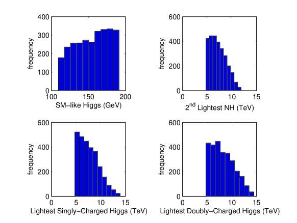
Figure 1: Frequency plot for the masses of the lightest Higgs bosons. The upper left plot shows the results for the SM-like Higgs boson, while the other plots show results for the lightest neutral, singly-charged and doubly-charged nonstandard Higgs bosons.

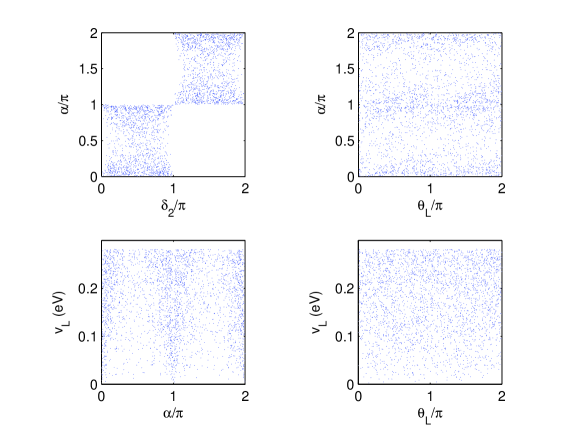
Figure 2: Various correlations between $\alpha$, $\delta_{2}$, $\theta_{L}$ and $v_{L}$.

Figures 1 and 2 show the results of our numerical analysis. The first of these shows a frequency plot of the lightest Higgs boson masses. While we have not imposed any direct mass constraints on the numerical results, the ranges described in Table 1 effectively limit the mass of the SM-like Higgs boson to be in the range $100~{}\mbox{GeV}\lesssim m_{\textrm{\scriptsize{SM}}}^{(0)}\lesssim 200$ GeV and those of all nonstandard Higgs bosons to be of order 4.7 TeV or greater. The scatter plots in Fig. 2 show various correlations between $v_{L}$, $\theta_{L}$, $\alpha$ and $\delta_{2}$. The correlation between $\alpha$ and $\delta_{2}$ is easily understood by examining the approximate relation in Eq. (26) – since $\alpha_{2}$, $\alpha_{3}$ and $\xi$ are all positive quantities, $\sin\delta_{2}$ and $\sin\alpha$ must have the same sign. The remaining three plots show various combinations of $\alpha$, $v_{L}$ and $\theta_{L}$, quantities that affect quark and lepton masses and mixings. In particular, notice that the phases $\alpha=\arg\left(\langle\phi_{2}^{0}\rangle\right)$ and $\theta_{L}=\arg\left(\langle\delta_{L}^{0}\rangle\right)$ are not constrained to be small. Also, $v_{L}$ is of order $0.1$ eV, which is phenomenologically viable. From these plots it does not appear that there are strong correlations between $\alpha$, $v_{L}$ and $\theta_{L}$. A numerical investigation of the case $v_{R}=50$ TeV yields similar plots (except that $v_{L}$ is reduced in magnitude because it scales as $1/v_{R}$).

Our numerical analysis also allows us to check the reliability of the approximate expressions for the mass-squared eigenvalues in Eqs. (42)-(49). The eigenvalues were computed numerically from the mass matrices and compared to the approximate expressions. For the singly- and doubly-charged Higgs bosons, the “exact” (numerical) values agreed with the approximate expressions to within a few parts in $10^{15}$ for $v_{R}=15$ TeV. The level of agreement for $m_{\rho_{3}}^{(0)2}$ was similar. Corrections for the other four neutral mass-squared eigenvalue expressions are described in the Appendix.

V Discussion and Conclusions

We have considered the Higgs sector of the minimal Left-Right model with explicit CP-violation in the Higgs potential in the “moderate” decoupling limit, i.e., when the scale set by the VEV of the right-handed Higgs field $v_{R}$ is in the range 15-50 TeV. This intermediate regime provides (at least in principle) testable effects of the remnants of RH symmetries in upcoming collider experiments. At the same time, inclusion of explicit CP violation in the Higgs potential allows for the generation of a viable spectrum of Higgs bosons containing one SM-like Higgs boson with mass of order the weak scale and several heavy neutral and charged Higgs bosons with masses of order $v_{R}$. Supplemented by an additional $U(1)$ horizontal symmetry, this model alleviates most of the fine-tuning effects associated with minimal LR models in the decoupling regime bgnr , resulting in an SM-like low energy effective theory. Yet, some small amount of fine-tuning is still required. We have also performed numerical simulations of the Higgs spectrum in our model, confirming our phenomenological analysis and the reliability of the adopted approximations. The power counting for the Higgs potential coupling constants provided by the broken $U(1)$ charge assignments also allows for the natural generation of neutrino masses in such a model.

*

Appendix A Goldstone Bosons and Approximate Masses

In this appendix we give exact expressions for the charged and neutral Goldstone bosons. These expressions are used to construct matrices that perform exact block diagonalizations for the singly-charged and neutral mass matrices, separating out the “zero” eigenvalues for the Goldstone modes. We also explain our procedure for obtaining the approximate mass-squared eigenvalues given in the text (Eqs. (42)-(49)).

A.1 Goldstone Bosons

The kinetic terms for the Higgs boson fields in the Lagrangian are given by duka

$${\cal L}_{\textrm{\scriptsize{kin}}}=\mbox{Tr}\left[\left(D_{\mu}\phi\right)^{\dagger}D^{\mu}\phi\right]+\mbox{Tr}\left[\left(D_{\mu}\Delta_{L}\right)^{\dagger}D^{\mu}\Delta_{L}\right]+\mbox{Tr}\left[\left(D_{\mu}\Delta_{R}\right)^{\dagger}D^{\mu}\Delta_{R}\right],$$ (50)

where covariant derivatives are defined as

$$D_{\mu}\phi = \partial_{\mu}\phi-\frac{ig}{2}W_{L\mu}^{a}\tau^{a}\phi+\frac{ig}{2}\phi W_{R\mu}^{a}\tau^{a}\;,$$ (51)

$$D_{\mu}\Delta_{L,R} = \partial_{\mu}\Delta_{L,R}-\frac{ig}{2}\left[W_{L,R\mu}^{a}\tau^{a},\Delta_{L,R}\right]-ig^{\prime}B_{\mu}\Delta_{L,R}\;.$$ (52)

Inserting Eqs. (7) and (16)-(19) into Eq. (50) yields the mass matrices for the gauge bosons, which may be diagonalized to obtain the physical mass eigenstates ($W_{1,2}^{\pm\mu}$, $Z_{1,2}$ and $A_{\mu}$) in terms of the original gauge bosons associated with $SU(2)_{L}\times SU(2)_{R}\times U(1)_{B-L}$ ($W_{L,R}^{\pm\mu}=\left(W_{L,R}^{1\mu}\mp iW_{L,R}^{2\mu}\right)/\sqrt{2}$, $W_{L,R}^{3\mu}$ and $B_{\mu}$). Equation (50) also yields bilinear couplings between the physical gauge bosons and various linear combinations of the Higgs fields. One such term is proportional to $igW_{1\mu}^{-}\partial^{\mu}G_{1}^{+}$, for example, and allows one to identify $G_{1}^{+}$ as a (would-be) Goldstone boson. Proceeding in this manner one obtains expressions for the two charged, orthogonalized Goldstone bosons,

$$G_{1}^{+} = \frac{1}{N_{1}^{+}}\left[\left(k_{1}\sin\zeta-k_{2}\cos\zeta\right)e^{-i\alpha}\phi_{1}^{+}+\left(k_{1}\cos\zeta-k_{2}\sin\zeta\right)\phi_{2}^{+}\right.$$ (53)

$$\left.~{}~{}~{}~{}~{}-\sqrt{2}v_{R}e^{-i\alpha}\sin\zeta\delta_{R}^{+}-\sqrt{2}v_{L}e^{-i\theta_{L}}\cos\zeta\delta_{L}^{+}\right],$$

$$G_{2}^{+} = \frac{1}{N_{2}^{+}}\left[\left(k_{1}\cos\zeta+k_{2}\sin\zeta\right)e^{-i\alpha}\phi_{1}^{+}+\left(-k_{1}\sin\zeta-k_{2}\cos\zeta\right)\phi_{2}^{+}\right.$$ (54)

$$\left.~{}~{}~{}~{}~{}-\sqrt{2}v_{R}e^{-i\alpha}\cos\zeta\delta_{R}^{+}+\sqrt{2}v_{L}e^{-i\theta_{L}}\sin\zeta\delta_{L}^{+}\right],$$

where $N_{1,2}^{+}$ are normalization constants and

$$\sin 2\zeta=\frac{2k_{1}k_{2}}{\left[(v_{R}^{2}-v_{L}^{2})^{2}+4k_{1}^{2}k_{2}^{2}\right]^{1/2}}\;.$$ (55)

We may also construct two other normalized, orthogonal linear combinations of the four fields $\phi_{1}^{+}$, $\phi_{2}^{+}$, $\delta_{R}^{+}$ and $\delta_{L}^{+}$,

$$\phi_{a}^{+} = \frac{1}{N_{a}^{+}}\left(e^{-i\alpha}\phi_{1}^{+}+r_{32}^{+}\phi_{2}^{+}+r_{33}^{+}e^{-i\alpha}\delta_{R}^{+}\right)\;,$$ (56)

$$\phi_{b}^{+} = \frac{1}{N_{b}^{+}}\left(r_{41}^{+}e^{-i\alpha}\phi_{1}^{+}+r_{42}^{+}\phi_{2}^{+}+r_{43}^{+}e^{-i\alpha}\delta_{R}^{+}+e^{-i\theta_{L}}\delta_{L}^{+}\right)\;,$$ (57)

where the $r_{ij}^{+}$ are simple functions of $k_{1}$, $k_{2}$, $v_{R}$ and $v_{L}$. (Forcing $\phi_{a}^{+}$ to be orthogonal to $G_{1}^{+}$ and $G_{2}^{+}$ determines $r_{32}^{+}$ and $r_{33}^{+}$; similarly, forcing $\phi_{b}^{+}$ to be orthogonal to $G_{1}^{+}$, $G_{2}^{+}$ and $\phi_{a}^{+}$ determines $r_{41}^{+}$, $r_{42}^{+}$ and $r_{43}^{+}$.) Putting the above expressions together, we form the unitary matrix ${\cal R}^{(+)}$ that relates the two bases,

$$\left(\begin{array}[]{c}G_{1}^{+}\\ G_{2}^{+}\\ \phi_{a}^{+}\\ \phi_{b}^{+}\\ \end{array}\right)={\cal R}^{(+)}\left(\begin{array}[]{c}\phi_{1}^{+}\\ \phi_{2}^{+}\\ \delta_{R}^{+}\\ \delta_{L}^{+}\\ \end{array}\right)\;.$$ (66)

The matrix ${\cal R}^{(+)}$ may be used to bring the $4\times 4$ singly-charged mass matrix into block-diagonal form, with a non-zero $2\times 2$ block in the lower-right,

$${\cal R}^{(+)*}{\cal M}_{+}^{2}{\cal R}^{(+)T}=\left(\begin{array}[]{cc}0&0\\ 0&{\cal M}_{+,2\times 2}^{2}\end{array}\right)\;.$$ (69)

One can similarly block-diagonalize the neutral mass matrix, although the diagonalization of the neutral gauge bosons is somewhat more involved than that of the charged gauge bosons. Furthermore, both $g$ and $g^{\prime}$ are involved, so that the physical mass eigenstates depend on the Weinberg angle ($\tan^{2}\theta_{W}=g^{\prime 2}/\left(g^{2}+g^{\prime 2}\right)$). Since our purpose is to block-diagonalize the neutral Higgs sector, and since the Higgs sector has no dependence on $\theta_{W}$, we will consider the (unphysical) limit $g^{\prime}/g\to 0$. This means our expressions for the Goldstone modes, while useful for diagonalization purposes, will not correspond to the actual combinations of Higgs bosons “eaten” by $Z_{1,2}$. Taking this limit, and proceeding as in the charged Goldstone case, we obtain

$$G_{1}^{0} = \frac{1}{N_{1}^{0}}\left[\left(\cos\phi+\sin\phi\right)\left(k_{1}\phi_{1}^{0i}-k_{2}\phi_{2}^{0i}\right)+2v_{R}\sin\phi\delta_{R}^{0i}-2v_{L}\cos\phi\delta_{L}^{0i}\right],$$ (70)

$$G_{2}^{0} = \frac{1}{N_{2}^{0}}\left[\left(\cos\phi-\sin\phi\right)\left(k_{1}\phi_{1}^{0i}-k_{2}\phi_{2}^{0i}\right)+2v_{R}\cos\phi\delta_{R}^{0i}+2v_{L}\sin\phi\delta_{L}^{0i}\right],$$ (71)

where

$$\sin 2\phi=-\frac{k_{1}^{2}+k_{2}^{2}}{\left[4(v_{R}^{2}-v_{L}^{2})^{2}+(k_{1}^{2}+k_{2}^{2})^{2}\right]^{1/2}}\;.$$ (72)

Defining orthogonal combinations

$$\phi_{a}^{0i} = \frac{1}{N_{a}^{0}}\left(r_{31}^{0}\phi_{1}^{0i}+\phi_{2}^{0i}\right)=\frac{1}{\sqrt{1+\xi^{2}}}\left(\xi\phi_{1}^{0i}+\phi_{2}^{0i}\right)\;,$$ (73)

$$\phi_{b}^{0i} = \frac{1}{N_{b}^{0}}\left(r_{41}^{0}\phi_{1}^{0i}+r_{42}^{0}\phi_{2}^{0i}+r_{43}^{0}\delta_{R}^{0i}+\delta_{L}^{0i}\right)$$ (74)

(where the $r_{ij}^{0}$ are again determined by forcing the various fields to be orthogonal), we construct the orthogonal matrix ${\cal R}^{(0)}$ that relates the two bases,

$$\left(\begin{array}[]{c}G_{1}^{0}\\ G_{2}^{0}\\ \phi_{a}^{0i}\\ \phi_{b}^{0i}\\ \end{array}\right)={\cal R}^{(0)}\left(\begin{array}[]{c}\phi_{1}^{0i}\\ \phi_{2}^{0i}\\ \delta_{R}^{0i}\\ \delta_{L}^{0i}\\ \end{array}\right)\;.$$ (83)

Defining an $8\times 8$ orthogonal matrix

$$\widetilde{\cal R}^{(0)}=\left(\begin{array}[]{cc}0&{\cal R}^{(0)}\\ \mathbf{1}_{4\times 4}&0\\ \end{array}\right),$$ (86)

we then have

$$\widetilde{\cal R}^{(0)}{\cal M}_{0}^{2}\widetilde{\cal R}^{(0)T}=\left(\begin{array}[]{cc}0&0\\ 0&{\cal M}_{0,6\times 6}^{2}\end{array}\right)\;,$$ (89)

where ${\cal M}_{0,6\times 6}^{2}$ is the symmetric $6\times 6$ mass matrix in the basis $\Phi_{0}^{T}=(\phi_{a}^{0i},\phi_{b}^{0i},\phi_{1}^{0r},\phi_{2}^{0r},\delta_{R}^{0r},\delta_{L}^{0r})$.

A.2 Approximate Mass-Squared Eigenvalues for Physical Higgs Bosons

Throughout this paper we assume that $v_{L}$ is small – of order $0.1$ eV or less – so that it is at a natural scale for neutrino masses. In this paper we also assume that the $\beta_{i}$ are suppressed through a horizontal symmetry, as indicated in Eq. (36), although any other scheme that introduces numerical scaling similar to Eq. (36) is indeed acceptable. Such a suppression of the $\beta_{i}$ leads naturally to the assumed small value for $v_{L}$, even if $v_{R}$ is only “moderately large” ($v_{R}\sim 15$ TeV), as indicated in Eqs. (37) and (41). It is important in our analysis that $v_{L}$ and the $\beta_{i}$ are not identically zero, since $v_{L}$ and its associated phase, $\theta_{L}$, are significant parameters for neutrino physics (see Eqs. (28) and (29)). Nevertheless, for calculating Higgs boson masses, it is an excellent approximation to consider the limit $\beta_{i},v_{L}\to 0$. This statement will be quantified in the following.

A.2.1 Doubly-Charged Higgs Bosons

The doubly-charged Higgs boson masses are determined by a $2\times 2$ Hermitian matrix. The off-diagonal elements in this matrix are proportional to $\rho_{4}v_{L}v_{R}$, $\beta_{1}k_{1}k_{2}$, $\beta_{2}k_{2}^{2}$ and $\beta_{3}k_{1}^{2}$. Assuming the scaling given in Eq. (36), the largest of these terms scales approximately as ${\cal O}(\epsilon^{2}\epsilon_{H}^{12}v_{R}^{2})$. The diagonal elements are of order $v_{R}^{2}$. Assuming no extreme accidental degeneracies in the diagonal elements, the corrections to the mass-squared eigenvalues due to the off-diagonal contributions are of order $\epsilon^{4}\epsilon_{H}^{24}v_{R}^{2}$. With $\epsilon\sim 0.016$ (for $v_{R}\sim 15$ TeV) and $\epsilon_{H}=0.3$, $\epsilon^{4}\epsilon_{H}^{24}\sim{\cal O}(10^{-20})$, and one can safely take the limit $\beta_{i},v_{L}\to 0$ for the off-diagonal elements. Taking this limit for the diagonal elements is also a very good approximation, since it only introduces a tiny error (of order $\epsilon^{4}\epsilon_{H}^{40}v_{R}^{2}\sim 10^{-28}\times v_{R}^{2}$). The approximate eigenvalues are thus simply the diagonal elements of the doubly-charged mass matrix in the limit $\beta_{i},v_{L}\to 0$. These approximate eigenvalues are denoted by $m_{\rho_{3}}^{(++)2}$ and $m_{\rho_{2}}^{(++)2}$ in Eqs. (48) and (49) and correspond to the fields $\delta_{L}^{++}$ and $\delta_{R}^{++}$, respectively. Our numerical work yields excellent agreement between these approximate expressions and the values obtained numerically by diagonalizing the full mass matrix – the values agree to within a few parts in $10^{15}$ in our numerical study with $v_{R}=15$ TeV.

A.2.2 Singly-Charged Higgs Bosons

For the singly-charged Higgs bosons it is also an excellent approximation to consider the limit $\beta_{i},v_{L}\to 0$. The justification for this approximation is somewhat more intricate to argue than in the doubly-charged case, but numerically it does appear to be an excellent approximation. (The numerical agreement for $v_{R}=15$ TeV is similar to that found in the doubly-charged case.) Taking the limit $\beta_{i},v_{L}\to 0$ in the mass matrix and in ${\cal R}^{(+)}$, one finds that $\delta_{L}^{+}$ decouples from the other three singly-charged Higgs fields, yielding

$${\cal M}_{+}^{2}\simeq\left(\begin{array}[]{cccc}m_{+}^{2}&m_{+}^{2}\xi e^{-i\alpha}&\frac{1}{\sqrt{2}}m_{+}^{2}\epsilon(1-\xi^{2})&0\\ &&&\\ m_{+}^{2}\xi e^{i\alpha}&m_{+}^{2}\xi^{2}&\frac{1}{\sqrt{2}}m_{+}^{2}\epsilon\xi(1-\xi^{2})e^{i\alpha}&0\\ &&&\\ \frac{1}{\sqrt{2}}m_{+}^{2}\epsilon(1-\xi^{2})&\frac{1}{\sqrt{2}}m_{+}^{2}\epsilon\xi(1-\xi^{2})e^{-i\alpha}&\frac{1}{2}m_{+}^{2}\epsilon^{2}(1-\xi^{2})^{2}&0\\ &&&\\ 0&0&0&m_{\rho_{3}}^{(+)^{2}}\\ \end{array}\right),$$ (97)

in the basis $(\phi_{1}^{+},\phi_{2}^{+},\delta_{R}^{+},\delta_{L}^{+})$, where

$$m_{+}^{2}=\frac{\alpha_{3}}{2}\frac{v_{R}^{2}}{\left(1-\xi^{2}\right)}$$ (98)

and where the approximate eigenvalue $m_{\rho_{3}}^{(+)^{2}}$ is given in Eq. (47). Performing the unitary transformation in Eq. (69) yields the approximate expression for the remaining non-zero eigenvalue, denoted $m_{\alpha_{3}}^{(+)^{2}}$ in Eq. (46). This latter eigenvalue is associated with the field $\phi_{a}^{+}\simeq\left[e^{-i\alpha}\phi_{1}^{+}+\xi\phi_{2}^{+}+\epsilon(1-\xi^{2})e^{-i\alpha}\delta_{R}^{+}/\sqrt{2}\right]/N_{a}^{+}$.

A.2.3 Neutral Higgs Bosons

Calculation of the approximate neutral mass-squared eigenvalues is simplified by once again taking the limit $\beta_{i},v_{L}\to 0$. We begin with the orthogonal rotation shown in Eq. (89) (taking the limit $v_{L}\to 0$ in $\widetilde{\cal R}^{(0)}$). This rotation yields the $6\times 6$ matrix ${\cal M}_{0,6\times 6}^{2}$, whose eigenvalues correspond to the six non-Goldstone Higgs bosons. In the limit $\beta_{i},v_{L}\to 0$, two of the fields ($\delta_{L}^{0r}$ and $\phi_{b}^{0i}\simeq\delta_{L}^{0i}$) decouple from the rest, allowing for immediate identification of their mass-squared eigenvalues. The eigenvalues are degenerate in this limit and are denoted by $m_{\rho_{3}}^{(0)^{2}}$ in Eq. (44). In numerical tests with $v_{R}=15$ TeV, the approximate expression for these eigenvalues has an accuracy comparable to those for the singly- and doubly-charged masses. Removing the entries corresponding to these two fields reduces the size of the remaining mass matrix to $4\times 4$. We call this matrix $\widetilde{\cal M}_{0,4\times 4}^{2}$ in the $(\phi_{a}^{0i},\phi_{1}^{0r},\phi_{2}^{0r},\delta_{R}^{0r})$ basis, where $\phi_{a}^{0i}$ is defined in Eq. (73). The procedure so far can be illustrated schematically as follows,

$${\cal M}_{0}^{2}~{}~{}~{}\stackrel{{\scriptstyle\beta_{i},v_{L}\to 0;\widetilde{\cal R}^{(0)}}}{{\Longrightarrow}}~{}~{}~{}{\cal M}_{0,6\times 6}^{2}~{}~{}~{}\stackrel{{\scriptstyle\textrm{\scriptsize{remove~{}}}\delta_{L}^{0r},\delta_{L}^{0i}}}{{\Longrightarrow}}~{}~{}~{}\widetilde{\cal M}_{0,4\times 4}^{2}\;.$$ (99)

The fields $\phi_{a}^{0i}$ and $\delta_{R}^{0r}$ are approximately mass eigenstates, with the remaining two approximate mass eigenstates being the following,

$$\phi_{\textrm{\scriptsize{SM}}} = \frac{1}{\sqrt{1+\xi^{2}}}\left(\phi_{1}^{0r}+\xi\phi_{2}^{0r}\right)\;,$$ (100)

$$\phi_{a}^{0r} = \frac{1}{\sqrt{1+\xi^{2}}}\left(-\xi\phi_{1}^{0r}+\phi_{2}^{0r}\right)\;.$$ (101)

Defining

$${\cal R}^{(0)}_{2}=\left(\begin{array}[]{cccc}0&\frac{1}{\sqrt{1+\xi^{2}}}&\frac{\xi}{\sqrt{1+\xi^{2}}}&0\\ 1&0&0&0\\ 0&-\frac{\xi}{\sqrt{1+\xi^{2}}}&\frac{1}{\sqrt{1+\xi^{2}}}&0\\ 0&0&0&1\\ \end{array}\right)\;,$$ (106)

the mass matrix in the basis $(\phi_{\textrm{\scriptsize{SM}}},\phi_{a}^{0i},\phi_{a}^{0r},\delta_{R}^{0r})$ is

$${\cal M}_{0,4\times 4}^{2}={\cal R}^{(0)}_{2}\widetilde{\cal M}_{0,4\times 4}^{2}{\cal R}^{(0)T}_{2}\sim\left(\begin{array}[]{cccc}\epsilon^{2}&\epsilon^{2}\xi&\epsilon^{2}\xi&\epsilon\alpha_{1},\epsilon\xi^{2}\\ \epsilon^{2}\xi&1&\epsilon^{2}\xi^{2}&\epsilon\xi\\ \epsilon^{2}\xi&\epsilon^{2}\xi^{2}&1&\epsilon\xi\\ \epsilon\alpha_{1},\epsilon\xi^{2}&\epsilon\xi&\epsilon\xi&1\\ \end{array}\right)v_{R}^{2}\;,$$ (111)

where the expression on the right gives the orders of magnitude of each of the entries, taking into account the scaling in Eq. (36). In the 1-4 and 4-1 entries we have explicitly included a term of order $\epsilon\alpha_{1}$, which could be of order $\epsilon$ if one chooses to take $\alpha_{1}\sim{\cal O}(1)$, but would be similar to other terms in that entry if one would choose $\alpha_{1}\sim{\cal O}(\xi^{2})$ or ${\cal O}(\epsilon^{2})$. In the following we assume that $\alpha_{1}\sim{\cal O}(\epsilon^{2})$.

The diagonal elements of ${\cal M}_{0,4\times 4}^{2}$ provide good estimates of the eigenvalues of the matrix. One could in principle compute corrections to these estimates by assuming that ${\cal M}_{0,4\times 4}^{2}$ is diagonalized by a “small” unitary rotation (i.e., by a unitary matrix that is essentially unity along the diagonal and that has small off-diagonal elements). Such an approach is complicated by the fact that the 2-2 and 3-3 elements in ${\cal M}_{0,4\times 4}^{2}$ are nearly degenerate. In fact, the difference between the two elements is of order $\epsilon^{2}\xi^{2}v_{R}^{2}$, which is the same order of magnitude as the 2-3 element of ${\cal M}_{0,4\times 4}^{2}$. This situation can lead to a large amount of mixing in the 2-3 block upon diagonalization of ${\cal M}_{0,4\times 4}^{2}$ and can also complicate matters somewhat for computing corrections to the 1-1 and 4-4 elements. We choose instead simply to use the diagonal elements to estimate the eigenvalues.

The approximate eigenvalue denoted $m_{\textrm{\scriptsize{SM}}}^{(0)2}$ in Eq. (42) corresponds to the field $\phi_{\textrm{\scriptsize{SM}}}$ in Eq. (100). Corrections to Eq. (100) are expected to be of order $\epsilon^{6}v_{R}^{2}$, $\epsilon^{4}\xi^{2}v_{R}^{2}$ and $\epsilon^{2}\xi^{4}v_{R}^{2}$, where we have assumed that the various Higgs potential coefficients scale as in Eq. (36) (except for $\alpha_{1}$, which is taken to be of order $\epsilon^{2}$). The approximate eigenvalue denoted $m_{\alpha_{3}}^{(0)2}$ in Eq. (43) corresponds to the nearly-degenerate fields $\phi_{a}^{0i}$ and $\phi_{a}^{0r}$. Corrections to Eq. (43) are expected to be of order $\epsilon^{2}\xi^{2}v_{R}^{2}$. Finally, the approximate eigenvalue corresponding to $\delta_{R}^{0r}$ is denoted by $m_{\rho_{1}}^{(0)2}$ in Eq. (45). Corrections to this expression are also expected to be of order $\epsilon^{2}\xi^{2}v_{R}^{2}$. In our numerical study with $v_{R}=15$ TeV we have compared the exact and approximate expressions for the various mass-squared eigenvalues. The numerical differences are consistent with the quoted corrections for $m_{\textrm{\scriptsize{SM}}}^{(0)2}$, $m_{\alpha_{3}}^{(0)2}$ and $m_{\rho_{1}}^{(0)2}$, although sometimes the corrections are larger due to accidental degeneracies or combinations of coefficients that occassionally give large enhancements. An example of the former effect occurs if the 2-2 and 4-4 or 3-3 and 4-4 elements of ${\cal M}_{0,4\times 4}^{2}$ are nearly degenerate. In that case, corrections to the respective eigenvalues can be of order $\epsilon\xi v_{R}^{2}$ instead of $\epsilon^{2}\xi^{2}v_{R}^{2}$. An example of the latter effect occurs for $m_{\textrm{\scriptsize{SM}}}^{(0)2}$, for which one of the leading corrections is proportional to $32\lambda_{3}^{2}\epsilon^{4}\xi^{2}v_{R}^{2}/\alpha_{3}$. If $\lambda_{3}\simeq 2$ and $\alpha_{3}\simeq 0.2$, this correction is of order $640\times\epsilon^{4}\xi^{2}v_{R}^{2}$.

References

• (1) J. C. Pati and A. Salam, Phys. Rev. D10, 275 (1974).
• (2) R. N. Mohapatra and J. C. Pati, Phys. Rev. D11, 566 (1975).
• (3) R. N. Mohapatra and J. C. Pati, Phys. Rev. D11, 2558 (1975).
• (4) G. Senjanovic and R. N. Mohapatra, Phys. Rev. D12, 1502 (1975).
• (5) R. N. Mohapatra, F. E. Paige, and D. P. Sidhu, Phys. Rev. D17, 2462 (1978).
• (6) G. Senjanovic, Nucl. Phys. B153, 334 (1979).
• (7) P. Duka, J. Gluza, and M. Zralek, Annals Phys. 280, 336 (2000), hep-ph/9910279.
• (8) E. M. B. Brahmachari and U. Sarkar, Phys. Rev. Lett. 91, 011801 (2003).
• (9) R. N. Mohapatra and G. Senjanovic, Phys. Lett. B79, 283 (1979).
• (10) M. A. B. Beg and H. S. B. Tsao, Phys. Rev. Lett. 41, 278 (1978).
• (11) R. N. Mohapatra and G. Senjanovic, Phys. Rev. Lett. 44, 912 (1980).
• (12) R. N. Mohapatra and G. Senjanovic, Phys. Rev. D23, 165 (1981).
• (13) G. C. Branco and L. Lavoura, Phys. Lett. B165, 327 (1985).
• (14) J. Basecq, J. Liu, J. Milutinovic, and L. Wolfenstein, Nucl. Phys. B272, 145 (1986).
• (15) J. F. Gunion, J. Grifols, A. Mendez, B. Kayser, and F. I. Olness, Phys. Rev. D40, 1546 (1989).
• (16) N. G. Deshpande, J. F. Gunion, B. Kayser, and F. I. Olness, Phys. Rev. D44, 837 (1991).
• (17) J. Gluza and M. Zralek, Phys. Rev. D51, 4695 (1995), hep-ph/9409225.
• (18) G. Barenboim, M. Gorbahn, U. Nierste, and M. Raidal, Phys. Rev. D65, 095003 (2002), hep-ph/0107121.
• (19) C. D. Froggatt and H. B. Nielsen, Nucl. Phys. B147, 277 (1979).
• (20) M. Leurer, Y. Nir, and N. Seiberg, Nucl. Phys. B398, 319 (1993), hep-ph/9212278.
• (21) O. Khasanov and G. Perez, Phys. Rev. D65, 053007 (2002), hep-ph/0108176.
• (22) K. Kiers, J. Kolb, J. Lee, A. Soni, and G.-H. Wu, Phys. Rev. D66, 095002 (2002), hep-ph/0205082.
• (23) A. Datta and A. Raychaudhuri, Phys. Rev. D62, 055002 (2000), hep-ph/9905421.
• (24) R. N. Mohapatra and P. B. Pal, Phys. Lett. B179, 105 (1986).
• (25) Particle Data Group, S. Eidelman et al., Phys. Lett. B592, 1 (2004).
• (26) ALEPH, A. Heister et al., Phys. Lett. B543, 1 (2002), hep-ex/0207054.
• (27) OPAL, G. Abbiendi et al., Phys. Lett. B526, 221 (2002), hep-ex/0111059.
• (28) DELPHI, J. Abdallah et al., Phys. Lett. B552, 127 (2003), hep-ex/0303026.
• (29) L3, P. Achard et al., Phys. Lett. B576, 18 (2003), hep-ex/0309076.
• (30) OPAL, G. Abbiendi et al., Phys. Lett. B577, 93 (2003), hep-ex/0308052.
• (31) G. Ecker and W. Grimus, Nucl. Phys. B258, 328 (1985).
• (32) M. E. Pospelov, Phys. Rev. D56, 259 (1997), hep-ph/9611422.
• (33) P. Ball, J. M. Frere, and J. Matias, Nucl. Phys. B572, 3 (2000), hep-ph/9910211.