Neutrino Oscillations in a Supersymmetric SO(10) Model with Type-III See-Saw Mechanism

Abstract:

The neutrino oscillations are studied in the framework of the minimal supersymmetric SO(10) model with Type-III see-saw mechanism by additionally introducing a number of SO(10) singlet neutrinos. The light Majorana neutrino mass matrix is given by a combination of those of the singlet neutrinos and the $SU(2)_{L}$ active neutrinos. The minimal SO(10) model gives an unambiguous Dirac neutrino mass matrix, which enables us to predict the masses and the other parameters for the singlet neutrinos. These predicted masses take the values accessible and testable by near future collider experiments under the reasonable assumptions. More comprehensive calculations on these parameters are also given.

1 Introduction

As pointed out in [1], we can construct, within the context of the standard model (SM), an operator which gives rise to the neutrino masses as

$${\cal L}_{\rm eff}=\frac{1}{\Lambda}\,(\ell_{L}H)^{T}C^{-1}(\ell_{L}H)\;.$$ (1)

Here $\ell$, $H$ are the lepton doublet and the Higgs doublet, $C$ is the charge conjugation operator and $\Lambda$ is the scale in which something new physics appears. In the usual see-saw mechanism (type-I see-saw mechanism) [2], the scale parameter $\Lambda$ is interpreted as the energy scale at which the right-handed neutrinos become active. In this paper, we explore the other possibility of type-III seesaw, introducing a set of singlet into the minimal supersymmetric standard model (MSSM). The motivations of this are as follows. One comes from the theoretical reason that string inspired $E_{6}$ models include SO(10) singlets as a matter content. The other does from the empirical reason that many indicate reduced coupling of neutrinos to the $Z^{0}$-boson in the framework of the SM or the SM with right-handed neutrinos [3, 4].

2 Type-III see-saw mechanism

We begin with reviewing the essential concept of the type-III see-saw mechanism proposed in the reference [5, 6, 7, 8, 9]. You can find a detailed study in [10]. In this model, in addition to the usual $SU(2)_{L}$ singlet $N=\nu_{R}$, we add a new SO(10) singlet neutrino “$S$”, which has a positive lepton number (+1),

$${\cal L}_{Y}=\int d^{2}\theta\left(Y_{\nu}~{}\overline{N}\ell_{L}\,H_{u}+Y_{s}~{}\overline{N}S_{L}\,H_{s}+\mu_{s}~{}S_{L}^{T}C^{-1}S_{L}\right)+h.c.\;,$$ (2)

where $H_{u}$ and $H_{s}$ are the $SU(2)_{L}$ doublet and singlet chiral superfields, respectively. This Lagrangian is written in a matrix form in the base with $\{\nu_{L},~{}N,~{}S_{L}\}$ as follows:

$$\left(\begin{array}[]{ccc}0&m_{D}^{T}&0\\ m_{D}&0&M_{D}^{T}\\ 0&M_{D}&\mu_{s}\end{array}\right)\;.$$ (3)

After the spontaneous symmetry breaking, they give masses to the neutrinos as

$$m_{D} = Y_{\nu}\left<H_{u}^{0}\right>~{},~{}~{}~{}M_{D}\ =\ Y_{s}\left<H_{s}\right>~{}.$$ (4)

Note that the $\mu_{s}$ term in the above breaks an originally existing global $U(1)_{L}$ and $U(1)_{\cal R}$ symmetries. Thus we can naturally expect it as a small value compared with the electroweak scale even around the keV scale, according to the following reason: when the $\mu_{s}$ term is arisen from the VEV of a singlet $\mu_{s}=\lambda\left<S^{\prime}\right>$, there appears a pseudo-NG boson, called Majoron $J=\Im S^{\prime}$ associated with the spontaneously broken $U(1)_{L}$ symmetry. Then the keV scale lepton number violation may lead to an interesting signature in the neutrinoless double beta decay [11] or becomes a possible candidate for the cold dark matter [12].

By integrating out $\nu_{R}$,

$$\frac{\partial{{\cal L}}}{\partial{N}}=m_{D}\nu_{L}+M_{D}S_{L}=0\;,$$ (5)

we obtain

$$S_{L}=-\left(\frac{m_{D}}{M_{D}}\right)\nu_{L}\;.$$ (6)

This means that the light neutrino mass eigenstate is a linear combination of two states $\nu_{L}$ and $S_{L}$ with the mixing angle $\epsilon\cong m_{D}/M_{D}$:

$$\nu_{\rm light}=\nu_{L}-\epsilon~{}S_{L}\;.$$ (7)

Such an extra mixing term is interesting when we try to explain the “NuTeV anomaly” through the heavy singlet neutrino contributions to the neutrino–nucleon scatterings [3, 4].

Putting Eq. (6) into Eq. (9), we get the effective light neutrino mass matrix as

$$M_{\nu}=\mu_{s}\left(\frac{m_{D}^{T}m_{D}}{M_{D}^{2}}\right)\;.$$ (8)

In general, adding three singlet neutrinos $\{S_{1},S_{2},S_{3}\}$, the effective light neutrino mass matrix can be written in the matrix form as

$$M_{\nu}=\left(M_{D}^{-1}m_{D}\right)^{T}\mu_{s}\left(M_{D}^{-1}m_{D}\right)\;.$$ (9)

This matrix is diagonalised by Maki-Nakagawa-Sakata (MNS) mixing matrix $U$ as

$$U^{T}M_{\nu}~{}U={\rm diag}(m_{1},m_{2},m_{3})\;.$$ (10)

An important fact is that the new physics scale has also the “see-saw structure” as

$$\Lambda\cong\frac{M_{D}^{2}}{\mu_{s}}\;.$$ (11)

Hence this mechanism is sometimes called as “double see-saw” mechanism. It’s not the actual see-saw type but the inverse see-saw form, because the small lepton number violating ( / $L$ ) scale $\mu_{s}$ would indicate the large scale.

Now we consider the general three generation cases. For simplicity, we assume that all $S_{i}$ have a common $\mu_{s}$ term. Then the light neutrino matrix is written as

$$\mu_{s}\,U^{T}m_{D}^{T}(M_{D}M_{D}^{T})^{-1}m_{D}U={\rm diag}(m_{1},m_{2},m_{3})\;,$$ (12)

that is,

$$M_{D}M_{D}^{T}=m_{D}U{\rm diag}\left(\frac{\mu_{s}}{m_{1}},\frac{\mu_{s}}{m_{2}},\frac{\mu_{s}}{m_{3}}\right)U^{T}m_{D}^{T}\;.$$ (13)

This symmetric combination can be diagonalised by a single unitary matrix ${\cal U}$

$${\cal U}^{T}~{}M_{D}M_{D}^{T}~{}{\cal U}={\rm diag}(M_{D1}^{2},M_{D2}^{2},M_{D3}^{2})\;.$$ (14)

Here we note that $\cal U$ includes three mixing angles $\theta^{\prime}_{1}$, $\theta^{\prime}_{2}$, $\theta^{\prime}_{3}$ and six phases ($\delta$, $\zeta_{2}^{L}$, $\zeta_{3}^{L}$, $\zeta_{1}^{R}$, $\zeta_{2}^{R}$, $\zeta_{3}^{R}$)

$${\cal U}=\left(\begin{array}[]{ccc}1&0&0\\ 0&e^{i\zeta_{2}^{L}}&0\\ 0&0&e^{i\zeta_{3}^{L}}\\ \end{array}\right)\left(\begin{array}[]{ccc}c_{3}c_{1}&c_{3}s_{1}&s_{3}e^{-i\delta}\\ -c_{2}s_{1}-s_{2}c_{1}s_{3}e^{i\delta}&c_{2}c_{1}-s_{2}s_{1}s_{3}e^{i\delta}&s_{2}c_{3}\\ s_{2}s_{1}-c_{2}c_{1}s_{3}e^{i\delta}&-s_{2}c_{1}-c_{2}s_{1}s_{3}e^{i\delta}&c_{2}c_{3}\\ \end{array}\right)\left(\begin{array}[]{ccc}e^{i\zeta_{1}^{R}}&0&0\\ 0&e^{i\zeta_{2}^{R}}&0\\ 0&0&e^{i\zeta_{3}^{R}}\\ \end{array}\right),$$ (15)

where $s_{i}:=\sin\theta^{\prime}_{i}$, $c_{i}:=\cos\theta^{\prime}_{i}$. You should not confuse these mixing angles with those of the MNS mixing matrix $U$ appearing in Eq. (34).

From this expression, we can obtain a prediction about masses and mixings for the heavier Dirac mass matrix $M_{D}$ by giving some informations about the light neutrino masses and mixings and the lighter Dirac mass matrix $m_{D}$.

3 Fermion masses in an SO(10) Model with a singlet

In order to make a prediction on the second Dirac neutrino mass matrix $M_{D}$, we need an information for the Yukawa couplings of $Y_{\nu}$. In this paper, we make the minimal SO(10) model extend to add a number of singlet, which preserves a precise information for $m_{D}$. We begin with a review of the minimal SUSY SO(10) model proposed in [13] and recently analysed in detail in references [14, 15, 16, 17, 18, 19, 20, 21]. Even when we concentrate our discussion on the issue of how to reproduce the realistic fermion mass matrices in the SO(10) model, there are lots of possibilities of the introduction of Higgs multiplets. The minimal supersymmetric SO(10) model includes only one 10 and one $\overline{\bf 126}$ Higgs multiplets in Yukawa couplings with 16 matter multiplets. Here, in addition to it, we introduce a number of SO(10) singlet chiral superfields ${\bf 1}$ as new matter multiplets . This additional singlet can provide a type-III see-saw mechanism as described in the previous section. In order to avoid a large triplet VEV for $\overline{\bf 126}_{H}$ unnecessary in type-III see-saw model, we use a $U(1)_{\cal R}$ symmetry. The corresponding $U(1)_{\cal R}$ charges are listed in Table 1. Then the relevant superpotential can be written as

fields	$U(1)_{\cal R}$ charges
${\bf 16}_{i}$	$-1$
${\bf 10}_{H}$	$+4$
$\overline{\bf 126}_{H}$	$+4$
$\overline{\bf 16}_{H}$	$+2$
${\bf 16}_{H}$	$-2$
${\bf 1}_{i}$	$+1$

Table 1: $U(1)_{\cal R}$ charges of the fields relevant for the quark and lepton mass matrices ($R[W]=+2$).

$$W_{Y}=Y_{10}^{ij}{\bf 16}_{i}{\bf 16}_{j}{\bf 10}_{H}+Y_{126}^{ij}{\bf 16}_{i}{\bf 16}_{j}\overline{{\bf 126}}_{H}+Y_{s}^{ij}{\bf 16}_{i}{\bf 1}_{j}\overline{{\bf 16}}_{H}+\mu_{s}{\bf 1}_{i}^{2}\;.$$ (16)

At low energy after the GUT symmetry breaking, the superpotential leads to

$$W = \left(Y_{10}^{ij}H_{10}^{u}+Y_{126}^{ij}H_{126}^{u}\right)u^{c}_{i}q_{j}+\left(Y_{10}^{ij}H_{10}^{d}+Y_{126}^{ij}H_{126}^{d}\right)d^{c}_{i}q_{j}$$ (17)

$$+ \left(Y_{10}^{ij}H_{10}^{u}-3Y_{126}^{ij}H_{126}^{u}\right)N_{i}{\ell}_{j}+\left(Y_{10}^{ij}H_{10}^{d}-3Y_{126}^{ij}H_{126}^{d}\right)e^{c}_{i}{\ell}_{j}$$

$$+ Y_{s}^{ij}N_{i}S_{j}H_{s}+\mu_{s}S_{i}^{2}\;,$$

where $H_{10}$ and $H_{126}$ correspond to the Higgs doublets in ${\bf 10}_{H}$ and $\overline{{\bf 126}}_{H}$. That is, we have two pairs of Higgs doublets. In order to keep the successful gauge coupling unification, we suppose that one pair of Higgs doublets (a linear combination of $H_{10}^{u,d}$ and $H_{126}^{u,d}$) is light while the other pair is heavy ($\simeq M_{\rm GUT}$). The light Higgs doublets are identified as the MSSM Higgs doublets ($H_{u}$ and $H_{d}$) and given by

$$H_{u}\ =\ \widetilde{\alpha}_{u}~{}H_{10}^{u}+\widetilde{\beta}_{u}~{}H_{126}^{u}\;;\quad H_{d}\ =\ \widetilde{\alpha}_{d}~{}H_{10}^{d}+\widetilde{\beta}_{d}~{}H_{126}^{d}\;,$$ (18)

where $\widetilde{\alpha}_{u,d}$ and $\widetilde{\beta}_{u,d}$ denote elements of the unitary matrix which rotate the flavour basis in the original model into the SUSY mass eigenstates. Omitting the heavy Higgs mass eigenstates, the low energy superpotential is described by only the light Higgs doublets $H_{u}$ and $H_{d}$ such that

$$W_{Y} = \left(\alpha^{u}Y_{10}^{ij}+\beta^{u}Y_{126}^{ij}\right)u^{c}_{i}q_{j}H_{u}\ +\ \left(\alpha^{d}Y_{10}^{ij}+\beta^{d}Y_{126}^{ij}\right)d^{c}_{i}q_{j}H_{d}$$ (19)

$$+ \left(\alpha^{u}Y_{10}^{ij}-3\beta^{u}Y_{126}^{ij}\right)N_{i}\ell_{j}H_{u}\ +\ \left(\alpha^{d}Y_{10}^{ij}-3\beta^{d}Y_{126}^{ij}\right)e_{i}^{c}\ell_{j}H_{d}$$

$$+ Y_{s}^{ij}N_{i}S_{j}H_{s}\ +\ \mu_{s}S_{i}^{2}\;,$$

where the formulas of the inverse unitary transformation of Eq. (18), $H_{10}^{u,d}=\alpha^{u,d}H_{u,d}+\cdots$ and $H_{126}^{u,d}=\beta^{u,d}H_{u,d}+\cdots$, have been used. Providing the Higgs VEV’s, $\langle H_{u}\rangle=v\sin\beta$ and $\langle H_{d}\rangle=v\cos\beta$ with $v\simeq 174$ [GeV], the Dirac mass matrices can be read off as

$$M_{u} = c_{10}M_{10}+c_{126}M_{126},$$

$$M_{d} = M_{10}+M_{126},$$

$$m_{D} = c_{10}M_{10}-3c_{126}M_{126},$$

$$M_{e} = M_{10}-3M_{126},$$ (20)

where $M_{u}$, $M_{d}$, $m_{D}$ and $M_{e}$ denote up-type quark, down-type quark, Dirac neutrino and charged-lepton mass matrices, respectively. Note that all the quark and lepton mass matrices are characterised by only two basic mass matrices, $M_{10}$ and $M_{126}$, and four complex coefficients $c_{10}$ and $c_{126}$. In addition to the above mass matrices the above model indicates the mass matrices,

$$M_{R} = c_{R}~{}M_{126}\;,$$

$$M_{L} = c_{L}~{}M_{126}\;,$$ (21)

together with $M_{D}$ given in Eq. (4). $c_{R}$ and $c_{L}$ correspond to the VEV’s of $({\bf 10},{\bf 1},{\bf 3})\subset{\overline{\bf 126}}$ and $({\overline{\bf 10}},{\bf 3},{\bf 1})\subset{\overline{\bf 126}}$, respectively [22]. If $M_{R}$, $M_{L}$, $M_{D}$ terms dominate, they are called Type-I, Type-II, and Type-III see-saw, respectively. In this paper, we consider the case $c_{R}\ =\ c_{L}\ =\ 0$, Type-III. Here $c_{R}=0$ means that the theory does not pass the Pati-Salam phase and is broken to the standard model directly.

The mass matrix formulas in Eq. (20) leads to the GUT relation among the quark and lepton mass matrices,

$$M_{e}=c_{d}\left(M_{d}+\kappa M_{u}\right)\;,$$ (22)

where

$$c_{d} = -\frac{3c_{10}+c_{126}}{c_{10}-c_{126}},$$ (23)

$$\kappa = -\frac{4}{3c_{10}+c_{126}}.$$ (24)

Without loss of generality, we can take the basis where $M_{u}$ is real and diagonal, $M_{u}=D_{u}$. Since $M_{d}$ is the symmetric matrix, it is described as $M_{d}=V_{\mathrm{CKM}}^{*}\,D_{d}\,V_{\mathrm{CKM}}^{\dagger}$ by using the CKM matrix $V_{\mathrm{CKM}}$ and the real diagonal mass matrix $D_{d}$. Considering the basis-independent quantities, $\mathrm{tr}[M_{e}^{\dagger}M_{e}]$, $\mathrm{tr}[(M_{e}^{\dagger}M_{e})^{2}]$ and $\mathrm{det}[M_{e}^{\dagger}M_{e}]$, and eliminating $|c_{d}|$, we obtain two independent equations,

$$\left(\frac{\mathrm{tr}[\widetilde{M_{e}}^{\dagger}\widetilde{M_{e}}]}{m_{e}^{2}+m_{\mu}^{2}+m_{\tau}^{2}}\right)^{2} = \frac{\mathrm{tr}[(\widetilde{M_{e}}^{\dagger}\widetilde{M_{e}})^{2}]}{m_{e}^{4}+m_{\mu}^{4}+m_{\tau}^{4}},$$ (25)

$$\left(\frac{\mathrm{tr}[\widetilde{M_{e}}^{\dagger}\widetilde{M_{e}}]}{m_{e}^{2}+m_{\mu}^{2}+m_{\tau}^{2}}\right)^{3} = \frac{\mathrm{det}[\widetilde{M_{e}}^{\dagger}\widetilde{M_{e}}]}{m_{e}^{2}\;m_{\mu}^{2}\;m_{\tau}^{2}},$$ (26)

where $\widetilde{M_{e}}\equiv V_{\mathrm{CKM}}^{*}\,D_{d}\,V_{\mathrm{CKM}}^{\dagger}+\kappa D_{u}$. With input data of six quark masses, three angles and one CP-phase in the CKM matrix and three charged-lepton masses, we can solve the above equations and determine $\kappa$ and $|c_{d}|$, but one parameter, the phase of $c_{d}$, is left undetermined [14, 15, 16]. With input data of six quark masses, three angles and one CP-phase in the CKM matrix and three charged lepton masses, we solve the above equations and determine $\kappa$. The original basic mass matrices, $M_{10}$ and $M_{126}$, are described by

$$M_{10} = \frac{3+|c_{d}|e^{i\sigma}}{4}V_{\mathrm{CKM}}^{*}\,D_{d}\,V_{\mathrm{CKM}}^{\dagger}+\frac{|c_{d}|e^{i\sigma}\kappa}{4}D_{u},$$ (27)

$$M_{126} = \frac{1-|c_{d}|e^{i\sigma}}{4}V_{\mathrm{CKM}}^{*}\,D_{d}\,V_{\mathrm{CKM}}^{\dagger}-\frac{|c_{d}|e^{i\sigma}\kappa}{4}D_{u},$$ (28)

as the functions of $\sigma$, the phase of $c_{d}$, with the solutions $|c_{d}|$ and $\kappa$ determined by the GUT relation.

Now let us solve the GUT relation and determine $|c_{d}|$ and $\kappa$. Since the GUT relation of Eq. (22) is valid only at the GUT scale, we first evolve the data at the weak scale to the corresponding quantities at the GUT scale with given $\tan\beta$ according to the renormalization group equations (RGE’s) and use them as input data at the GUT scale. Note that it is non-trivial to find the solution of the GUT relation since the number of the free parameters (fourteen) is almost the same as the number of inputs (thirteen). The solution of the GUT relation exists only if we take appropriate input parameters. Taking the experimental data at the $M_{Z}$ scale [23], we get the following values for charged fermion masses and the CKM matrix at the GUT scale, $M_{\rm GUT}$ with $\tan\beta=10$:

$$m_{u}=0.000980\;,\;\;m_{c}=0.285\;,\;\;m_{t}=113,$$

$$m_{d}=0.00135\;,\;\;m_{s}=0.0201\;,\;\;m_{b}=0.996,$$

$$m_{e}=0.000326\;,\;\;m_{\mu}=0.0687\;,\;\;m_{\tau}=1.17,$$

and

$$V_{\mathrm{CKM}}(M_{G})=\left(\begin{array}[]{ccc}0.975&0.222&-0.000940-0.00289i\\ -0.222-0.000129i&0.974+0.000124i&0.0347\\ 0.00864-0.00282i&-0.0337-0.000647i&0.999\end{array}\right)\;$$ (32)

in the standard parameterisation. The signs of the input fermion masses have been chosen to be $(m_{u},m_{c},m_{t})=(+,-,+)$ and $(m_{d},m_{s},m_{b})=(-,-,+)$. By using these outputs at the GUT scale as input parameters, we can solve Eqs. (25) and (26) and find a solution:

$$\kappa=-0.0103+0.000606i\;,$$

$$|c_{d}|=6.32\;.$$ (33)

Once these parameters, $|c_{d}|$ and $\kappa$, are determined, we can describe all the fermion mass matrices as a functions of $\sigma$ from the mass matrix formulas of Eqs. (20), (27) and (28). Thus in the minimal SO(10) model we have almost unambiguous Dirac neutrino mass matrix $m_{D}$ and, therefore, we can obtain the informations on $M_{D}$ from the neutrino experiments via $M_{\nu}=(M_{D}^{-1}m_{D})^{T}\mu_{s}(M_{D}^{-1}m_{D})$ as in Eq. (9).

Now we proceed to the numerical calculation of $M_{D}$ from the well-confirmed neutrino oscillation data. The MNS mixing matrix $U$ in the standard parametrization is

$$U=\left(\begin{array}[]{ccc}c_{13}c_{12}&c_{13}s_{12}e^{i\varphi_{2}}&s_{13}e^{i(\varphi_{1}-\delta)}\\ (-c_{23}s_{12}-s_{23}c_{12}s_{13}e^{i\delta})e^{-i\varphi_{2}}&c_{23}c_{12}-s_{23}s_{12}s_{13}e^{i\delta}&s_{23}c_{13}e^{i(\varphi_{1}-\varphi_{2})}\\ (s_{23}s_{12}-c_{23}c_{12}s_{13}e^{i\delta})e^{-i\varphi_{1}}&(-s_{23}c_{12}-c_{23}s_{12}s_{13}e^{i\delta})e^{-i(\varphi_{1}-\varphi_{2})}&c_{23}c_{13}\\ \end{array}\right)\;,$$ (34)

where $s_{ij}:=\sin\theta_{ij}$, $c_{ij}:=\cos\theta_{ij}$ and $\delta$, $\varphi_{1}$, $\varphi_{2}$ are the Dirac phase and the Majorana phases, respectively. Recent KamLAND data tells us that

$$\Delta m^{2}_{\oplus} = \Delta m^{2}_{32}\ =\ 2.1\times 10^{-3}\;\;{\mathrm{eV}}^{2}\;,$$

$$\sin^{2}\theta_{\oplus} = 0.5\;,$$

$$\Delta m^{2}_{\odot} = \left|\Delta m^{2}_{21}\right|\ =\ 8.3\times 10^{-5}\;\;{\mathrm{eV}}^{2}\;,$$

$$\sin^{2}\theta_{\odot} = 0.28\;,$$

$$|U_{e3}|^{2} < 0.061\;.$$ (35)

For simplicity we take $U_{e3}=0$. Note that we can take both signs of $\Delta m^{2}_{21}$, $\Delta m^{2}_{21}>0$ or $\Delta m^{2}_{21}<0$. The former is called normal hierarchy, the latter is called inverted hierarchy. Here we adopt the former case, and take the lightest neutrino mass eigenvalue as $m_{\ell}=10^{-3}\;{\rm[eV]}$. Then the mass eigenvalues are written as

$$m_{1} = m_{\ell}\;,$$

$$m_{2} = \sqrt{m_{\ell}^{2}+\Delta m^{2}_{\oplus}}\;,$$

$$m_{3} = \sqrt{m_{\ell}^{2}+\Delta m^{2}_{\oplus}+\Delta m^{2}_{\odot}}\;.$$ (36)

For the light Dirac neutrino mass matrix $m_{D}$, we input the SO(10) predicted one as was done in the previous section. However, unlike the case of minimal SO(10) GUT model, we can not fix $\sigma$. So we can obtain the heavy Dirac neutrino mass matrix $M_{D}$ as a function of $\mu_{s}$ and the three undetermined parameters, $\sigma$, two Majorana phases $\varphi_{1}$ and $\varphi_{2}$. For example, for fixed $\mu_{s}=1~{}{\rm[keV]}$ (For the implication of this value, see the remarks below Eq. (4).) and $\varphi_{1}=\varphi_{2}=0$, we get a prediction for the mass spectra of $M_{D}$. The dependences on the parameters $\sigma$ and $U_{e3}$ for fixed $\sigma=\pi$ are depicted in Fig. 1. These values are allowed by the present experiments [24] and are accessible and testable by the Large Hadron Collider (LHC) at CERN, in which we are able to discover new particles with masses up to $\lesssim 7$ [TeV] [25].

      

      

Figure 1: The predicted mass spectra of an additional singlet neutrino $M_{Di}~{}(i=1-3)$. The top panel represents three mass eigenvalues as a function of $\sigma$, the second and the third panels are the lightest and the second lightest masses as a function of $U_{e3}$ for fixed $\sigma=\pi$.

Of course, these values depend on the ambiguous assumptions taken above. We may take another strategy adopted in [21]. As shown in the paper [21], we repeat the substitution of the normally-distributed random numbers which give the experimental values [26]:

$$\left|{m_{u}\left({2~{}{\rm{GeV}}}\right)}\right| = 2.9\pm 0.6~{}{\rm{[MeV]}},\quad\left|{m_{d}\left({2~{}{\rm{GeV}}}\right)}\right|=5.2\pm 0.9~{}{\rm{[MeV]}},$$ (37)

$$\left|{m_{s}\left({2~{}{\rm{GeV}}}\right)}\right| = 99\pm 16~{}{\rm{[MeV]}},\quad\left|{m_{c}\left({m_{c}}\right)}\right|=1.0-1.4~{}{\rm{[GeV]}},$$ (38)

$$m_{b}\left({m_{b}}\right) = 4.0-4.5~{}{\rm{[GeV]}},\quad m_{t}^{{\rm{direct}}}=174.3\pm 5.1~{}{\rm{[GeV]}},$$ (39)

$$\left|{m_{e}^{{\rm{pole}}}}\right| = {\rm{0.510998902}}\pm{\rm{0.000000021~{}[MeV]}},$$ (40)

$$\left|{m_{\mu}^{{\rm{pole}}}}\right| = {\rm{105.658357}}\pm{\rm{0.00005,}}\quad m_{\tau}^{{\rm{pole}}}={\rm{1776.99}}\pm{\rm{0.29~{}[MeV]}},$$ (41)

$$\sin\theta_{12} = 0.2229\pm 0.0022,\quad\sin\theta_{23}=0.0412\pm 0.0020,$$ (42)

$$\sin\theta_{13} = 0.0036\pm 0.0007,\quad\delta=\left({59\pm 13}\right)^{\circ}$$ (43)

for the quark and charged lepton masses and the CKM mixing and the Dirac phase parameters 10,000 times. On the other hand, about the remaining parameters, we assume Eq. (35), $m_{1}=10^{-3}$ [eV] and $U_{e3}=0$ at the GUT scale, and Majorana phases and $\sigma$ move from $0$ to $2\pi$ in 8 equal intervals. Namely, we scan the possible ranges of undetermined parameters $\sigma$, $\varphi_{1}$, $\varphi_{2}$ and plotted the three masses of $M_{D}$, the three mixing angles and five phases of ${\cal U}$ which diagonalises the mass matrix $M_{D}$ in the basis where $M_{e}$ is real diagonal in Figs. 2–5. Here we calculated the distributions for sixteen sets of possible combinations of mass signatures of up-type and down-type quarks. Figure 1 corresponds to the blue solid line of Figure 2 with $\mu_{s}=1$ [KeV].

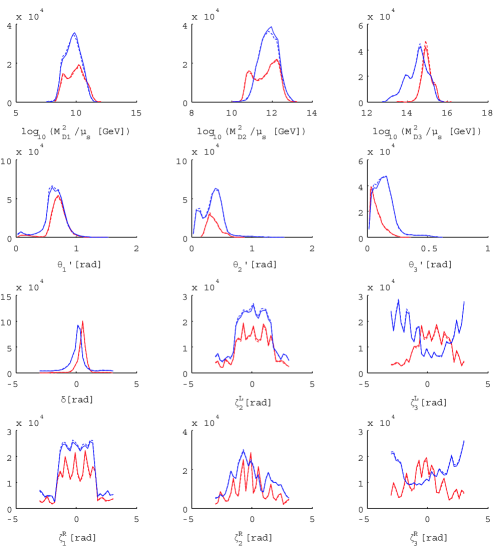
Figure 2: The distributions of the predicted mass ratios, mixing angles and phases for $M_{D}$. The signs of each mass eigenvalues are chosen as follows: The red solid line is $(m_{u},m_{c},m_{t})=(+,+,+);~{}(m_{d},m_{s},m_{b})=(+,+,+)$, the red dotted one is $(m_{u},m_{c},m_{t})=(-,+,+);~{}(m_{d},m_{s},m_{b})=(+,+,+)$, the blue solid one is $(m_{u},m_{c},m_{t})=(+,-,+);~{}(m_{d},m_{s},m_{b})=(-,-,+)$ and the blue dotted one is $(m_{u},m_{c},m_{t})=(-,-,+);~{}(m_{d},m_{s},m_{b})=(-,-,+)$.

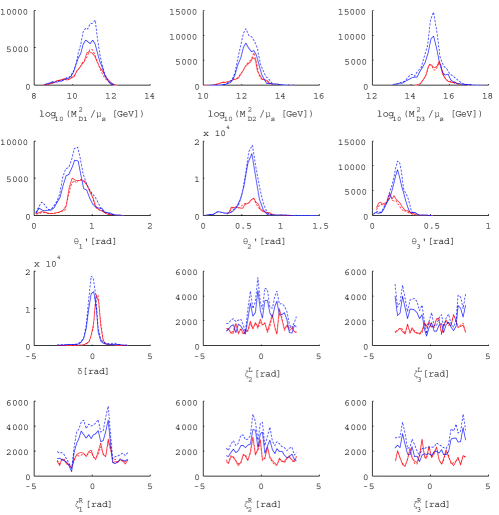
Figure 3: The same distributions as Figure 2 but the signs of each mass eigenvalues are chosen as follows: The red solid line is $(m_{u},m_{c},m_{t})=(+,-,+);~{}(m_{d},m_{s},m_{b})=(+,+,+)$, the red dotted one is $(m_{u},m_{c},m_{t})=(-,-,+);~{}(m_{d},m_{s},m_{b})=(+,+,+)$, the blue solid one is $(m_{u},m_{c},m_{t})=(+,+,+);~{}(m_{d},m_{s},m_{b})=(-,-,+)$ and the blue dotted one is $(m_{u},m_{c},m_{t})=(-,+,+);~{}(m_{d},m_{s},m_{b})=(-,-,+)$.

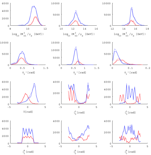
Figure 4: The same distributions as Figure 2 but the signs of each mass eigenvalues are chosen as follows: The red solid line is $(m_{u},m_{c},m_{t})=(+,+,+);~{}(m_{d},m_{s},m_{b})=(-,+,+)$, the red dotted one is $(m_{u},m_{c},m_{t})=(-,+,+);~{}(m_{d},m_{s},m_{b})=(-,+,+)$, the blue solid one is $(m_{u},m_{c},m_{t})=(+,-,+);~{}(m_{d},m_{s},m_{b})=(+,-,+)$ and the blue dotted one is $(m_{u},m_{c},m_{t})=(-,-,+);~{}(m_{d},m_{s},m_{b})=(+,-,+)$.

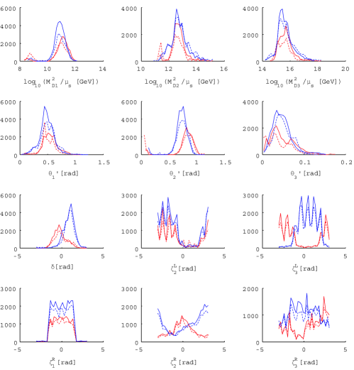
Figure 5: The same distributions as Figure 2 but the signs of each mass eigenvalues are chosen as follows: The red solid line is $(m_{u},m_{c},m_{t})=(+,-,+);~{}(m_{d},m_{s},m_{b})=(-,+,+)$, the red dotted one is $(m_{u},m_{c},m_{t})=(-,-,+);~{}(m_{d},m_{s},m_{b})=(-,+,+)$, the blue solid one is $(m_{u},m_{c},m_{t})=(+,+,+);~{}(m_{d},m_{s},m_{b})=(+,-,+)$ and the blue dotted one is $(m_{u},m_{c},m_{t})=(-,+,+);~{}(m_{d},m_{s},m_{b})=(+,-,+)$.

Finally, it is remarkable to say that the see-saw mechanism itself (or the types of it) can never been proofed and all the models should take care of all the types of the see-saw mechanism including the alternatives to it [27, 28]. The test of all these models is due to the applications to the other phenomelogical consequences, for example, the lepton flavour violating processes and so on [29, 30].

4 Summary

In this paper, we have constructed an SO(10) model in which the smallness of the neutrino masses are explained in terms of the type-III see-saw mechanism. To evaluate the parameters related to the singlet neutrinos, we have used the minimal SUSY SO(10) model. This model can simultaneously accommodate all the observed quark-lepton mass matrix data with appropriately fixed free parameters. Especially, the neutrino-Dirac-Yukawa coupling matrix are completely determined. Using this Yukawa coupling matrix, we have calculated the masses and mixings for the not-so-heavy singlet neutrinos. The obtained ranges of the mass of $M_{D}$ is interesting since they are testable by a forthcoming LHC experiment.

References

[1]
S. Weinberg,
Phys. Rev. Lett. 43, 1566 (1979).
[2]
T. Yanagida, in Proceedings of the workshop
on the Unified Theory and Baryon Number in the Universe,
edited by O. Sawada and A. Sugamoto (KEK, Tsukuba, 1979);
M. Gell-Mann, P. Ramond, and R. Slansky,
in Supergravity, edited by D. Freedman and P. van Niewenhuizen
(north-Holland, Amsterdam 1979);
R. N. Mohapatra and G. Senjanović,
Phys. Rev. Lett. 44, 912 (1980).
[3]
G. P. Zeller et al. [NuTeV Collaboration],
Phys. Rev. Lett. 88, 091802 (2002)
[Erratum-ibid. 90, 239902 (2003)]
[arXiv:hep-ex/0110059];
The theoretical explanations of this anomaly by including
heavy singlet neutrinos are given in [4].
[4]
T. Takeuchi,
[arXiv:hep-ph/0209109];
W. Loinaz, N. Okamura, T. Takeuchi and L. C. R. Wijewardhana,
Phys. Rev. D 67, 073012 (2003)
[arXiv:hep-ph/0210193];
W. Loinaz, N. Okamura, S. Rayyan, T. Takeuchi and L. C. R. Wijewardhana,
Phys. Rev. D 70, 113004 (2004)
[arXiv:hep-ph/0403306].
[5]
E. Witten,
Nucl. Phys. B 268, 79 (1986).
[6]
R. N. Mohapatra,
Phys. Rev. Lett. 56 (1986) 561.
[7]
R. N. Mohapatra and J. W. F. Valle,
Phys. Rev. D 34, 1642 (1986).
[8]J. W. F. Valle, in
NUCLEAR BETA DECAYS AND NEUTRINO: proceedings.
Edited by T. Kotani, H. Ejiri, E. Takasugi.
Singapore, World Scientific, 1986. 542p.
[9]
S. M. Barr,
Phys. Rev. Lett. 92, 101601 (2004)
[arXiv:hep-ph/0309152].
[10]
I. Melo,
[arXiv:hep-ph/9612488].
[11]
Z. G. Berezhiani, A. Y. Smirnov and J. W. F. Valle,
Phys. Lett. B 291, 99 (1992)
[arXiv:hep-ph/9207209].
[12]
V. Berezinsky and J. W. F. Valle,
Phys. Lett. B 318, 360 (1993)
[arXiv:hep-ph/9309214].
[13]
K. S. Babu and R. N. Mohapatra,
Phys. Rev. Lett. 70, 2845 (1993)
[arXiv:hep-ph/9209215].
[14]
K. Matsuda, Y. Koide and T. Fukuyama,
Phys. Rev. D 64, 053015 (2001)
[arXiv:hep-ph/0010026].
[15]
K. Matsuda, Y. Koide, T. Fukuyama and H. Nishiura,
Phys. Rev. D 65, 033008 (2002)
[Erratum-ibid. D 65, 079904 (2002)]
[arXiv:hep-ph/0108202];
[16]
T. Fukuyama and N. Okada,
JHEP 0211, 011 (2002)
[arXiv:hep-ph/0205066].
[17]
H. S. Goh, R. N. Mohapatra and S. P. Ng,
Phys. Lett. B 570, 215 (2003)
[arXiv:hep-ph/0303055].
[18]
H. S. Goh, R. N. Mohapatra and S. P. Ng,
Phys. Rev. D 68, 115008 (2003)
[arXiv:hep-ph/0308197].
[19]
B. Bajc, G. Senjanović and F. Vissani,
Phys. Rev. Lett. 90, 051802 (2003)
[arXiv:hep-ph/0210207].
[20]
B. Dutta, Y. Mimura and R. N. Mohapatra,
Phys. Rev. D 69, 115014 (2004)
[arXiv:hep-ph/0402113].
[21]
K. Matsuda,
Phys. Rev. D 69, 113006 (2004)
[arXiv:hep-ph/0401154].
[22]
K. Matsuda, T. Fukuyama and H. Nishiura,
Phys. Rev. D 61, 053001 (2000)
[arXiv:hep-ph/9906433].
[23]
H. Fusaoka and Y. Koide,
Phys. Rev. D 57, 3986 (1998)
[arXiv:hep-ph/9712201].
[24]
P. Achard et al. [L3 Collaboration],
Phys. Lett. B 517, 67 (2001)
[arXiv:hep-ex/0107014].
[25]
S. N. Gninenko, M. M. Kirsanov, N. V. Krasnikov and V. A. Matveev,
[arXiv:hep-ph/0301140].
[26]
S. Eidelman et al. [Particle Data Group],
Phys. Lett. B 592, 1 (2004).
[27]
H. Murayama,
Nucl. Phys. Proc. Suppl. 137, 206 (2004)
[arXiv:hep-ph/0410140].
[28]
A. Y. Smirnov,
[arXiv:hep-ph/0411194].
[29]
F. Deppisch and J. W. F. Valle,
[arXiv:hep-ph/0406040].
[30]
A. Ilakovac and A. Pilaftsis,
Nucl. Phys. B 437, 491 (1995)
[arXiv:hep-ph/9403398].