Simulations of the End of Supersymmetric Hybrid Inflation and Non-Topological Soliton Formation

Abstract

We present two- and three-dimensional simulations of the growth of quantum fluctuations of the scalar fields in supersymmetric hybrid inflation models. For a natural range of couplings, sub-horizon quantum fluctuations undergo rapid growth due to scalar field dynamics, resulting in the formation of quasi-stable non-topological solitons (inflaton condensate lumps) which dominate the post-inflation era.

¹mattb@amtp.liv.ac.uk ²j.mcdonald@lancaster.ac.uk

1 Introduction

Hybrid inflation models [2] are a promising class of model, having a classically flat inflaton potential without requiring fine-tuning of coupling constants. In order to control radiative corrections to the inflaton potential, supersymmetric (SUSY) hybrid inflation models are favoured [3, 4, 5]. D-term hybrid inflation models are of particular interest, since they naturally account for the absence of order $H^{2}$ corrections to the inflaton mass squared term coming from non-renormalisable interactions with non-zero F-terms. However, in spite of requiring fine-tuning to eliminate order $H^{2}$ corrections, several F-term hybrid inflation models have also been proposed. In light of recent reconsideration of the issue of fine-tuning in SUSY models and the idea of ’split supersymmetry’ [6], such models may still play an important role.

An important issue is the process by which inflation ends and the Universe reheats. It is known that the end of inflation and reheating in hybrid inflation is dominated by the non-linear dynamics of the scalar fields responsible for inflation [7, 8, 9]. Sub-horizon quantum fluctuations are rapidly amplified by scalar field dynamics once the symmetry breaking transition ending inflation occurs, becoming effectively classical modes [7, 8]. The energy density at the end of inflation rapidly becomes dominated by spatial fluctuations of the inflaton. For the case of D-term hybrid inflation, the rapid growth of the perturbations is expected to dominate the energy density for $\lambda\;^{>}_{\sim}\;0.1g$ [10]. Similar dynamics may be observed in models of tachyonic inflation [11].

What is the subsequent evolution of this inhomogeneous scalar field? There are two possible outcomes. The growth of the spatial perturbations of the inflaton could result in scalar field waves which scatter from each other, dispersing the energy of the initially highly inhomogeneous state [7, 8]. Alternatively, the growth of the spatial perturbations might continue, resulting in the formation of non-topological solitons corresponding to inflaton breathers [9] (also known as oscillons [13]). This was first suggested in an alternative view of the end of hybrid inflation, inflaton condensate fragmentation [9], which was based upon perturbing a homogeneous inflaton condensate assumed to form immediately after the end of hybrid inflation. In [9] the non-topological solitons were called inflaton condensate lumps. Their existence can be understood as the result of an effective attractive interaction between the inflaton scalars due to the symmetry breaking field [9]. Although the assumption of a homogeneous inflaton condensate is violated by the rapid growth of quantum fluctuations within a few coherent oscillation periods, the possibility that spatial perturbations could form non-topological solitons remains. Such objects were subsequently observed in a numerical simulation of the phase transition in hybrid inflation [14]. Oscillons such as inflaton condensate lumps are known to be quasi-stable, having a lifetime much longer than the period of the inflaton coherent oscillations [13]. They decay by a slow radiation of scalar field waves. For the case of the effective theory associated with SUSY hybrid inflation models, the lifetime of the inflaton condensate lumps is $10^{3}-10^{4}$ times the oscillation period [15].

The possibility of non-topological soliton formation at the end of SUSY hybrid inflation is strengthened by the existence of stable Q-ball solutions of the scalar field equations of D- and F-term inflation [16]. These are two-field Q-ball solutions, composed of a complex inflaton field and a real symmetry breaking field. They carry a conserved global charge associated with the inflaton. As a result, it is possible that SUSY hybrid inflation could end by initially forming neutral non-topological solitons which subsequently decay to pairs of stable Q-balls of opposite global charge. The formation of neutral condensate lumps which decay to Q-ball pairs has been observed numerically in the context of Affleck-Dine condensates along MSSM flat directions [17]. (See also [18].) It occurs because the initially neutral condensate lumps are unstable with respect to growth of perturbations of the phase of the complex scalar field, resulting in the formation of an energetically preferred state consisting of a stable Q-ball, anti-Q-ball pair. This is likely to be a generic feature of the evolution of quasi-stable neutral condensate lumps whenever a related stable Q-ball solution exists.

Thus there exists the possibility that the post-inflation era of SUSY hybrid inflation models will be dominated by Q-balls containing most of the energy of the Universe. Whether this happens depends upon whether the inhomogeneous state of the Universe immediately following inflation evolves into quasi-stable neutral condensate lumps or simply disperses as scalar field waves. In this paper we report the results of a numerical simulation of the growth and evolution of quantum fluctuations of the scalar fields in SUSY hybrid inflation models. The growth of quantum fluctuations into classical fluctuations is studied using the equivalent classical stochastic field method [19], which replaces the quantum field theory by an equivalent classical field theory with a classical probability distribution for the initial conditions. We focus on the case of D-term inflation. The results for F-term inflation are likely to be similar to those of D-term inflation for a particular choice of the D-term inflation model couplings.

The paper is organised as follows. In Section 2 we review SUSY hybrid inflation models and the scalar field equations. In Section 3 we discuss the initial conditions and details of the numerical simulation. In Section 4 we present the results of 2-D and 3-D simulations of the evolution of the scalar fields. In Section 5 we discuss a scaling property of the D-term inflation field equations and the dependence of our numerical results on the coupling constants. In Section 6 we compare our results with earlier numerical simulations. In Section 7 we present our conclusions. In the Appendix we review the equivalent classical stochastic field method.

2 SUSY Hybrid Inflation Models

The minimal D-term inflation model is described by the superpotential [3]

$$\mbox{$$}W=\lambda S\Phi_{+}\Phi_{-}~{},\vspace{\undereqskip}$$ (1)

where $S$ is the inflaton, $\Phi_{\pm}$ are fields with charges $\pm 1$ with respect to a Fayet-Iliopoulos $U(1)_{FI}$ gauge symmetry, $\xi>0$ is the Fayet-Iliopoulos term ($\xi^{1/2}=8.5\times 10^{15}{\rm\ GeV}$ [5]) and $g$ is the $U(1)_{FI}$ gauge coupling. The scalar potential is given by

$$\mbox{$$}V=\lambda^{2}|S|^{2}\left(|\Phi_{+}|^{2}+|\Phi_{-}|^{2}\right)+\lambda^{2}|\Phi_{+}|^{2}|\Phi_{-}|^{2}+\frac{g^{2}}{2}\left(|\Phi_{+}|^{2}-|\Phi_{-}|^{2}+\xi\right)^{2}~{}.\vspace{\undereqskip}$$ (2)

Once $|S|<s_{c}/\sqrt{2}=g\xi^{1/2}/\lambda$, $\Phi_{-}$ develops a non-zero expectation value, breaking the $U(1)_{FI}$ symmetry and ending inflation.

The simplest F-term inflation model is described by the superpotential [4]

$$\mbox{$$}W=\frac{\eta}{2}S\left(\Phi^{2}-\mu^{2}\right)~{},\vspace{\undereqskip}$$ (3)

where $S$ is the inflaton and $\Phi$ is the field which terminates inflation. $\mu^{2}$ and $\eta$ may be chosen real and positive. The scalar potential is then

$$\mbox{$$}V=\eta^{2}|S|^{2}|\Phi|^{2}+\frac{\eta^{2}}{4}|\Phi^{2}-\mu^{2}|^{2}~{}.\vspace{\undereqskip}$$ (4)

For the case of real scalar fields, the F-term scalar field equations become equivalent to the D-term equations in the limit where $\Phi_{+}=0$ and $\lambda=\sqrt{2}g$.

The superpotentials Eq. (1) and Eq. (3) are invariant with respect to an R-symmetry under which only $S$ transforms, which manifests itself as a global $U(1)$ symmetry of the scalar potential, $S\rightarrow e^{i\alpha}S$. It is this symmetry which is responsible for the conserved global charge of the hybrid inflation Q-balls [16].

In the following we will focus on the minimal D-term inflation model. We expect the end of inflation in F-term inflation models to be similar to D-term inflation in the case $\lambda=\sqrt{2}g$, up to the effect of $U(1)_{FI}$ symmetry breaking and cosmic string formation, which our results indicate are of secondary importance to the evolution of the energy density. During inflation, the inflaton evolves due to the 1-loop effective potential, $\Delta V(|S|,|\Phi_{-}|)$ . This determines its rate of rolling at the end of inflation, an important initial condition for the subsequent non-linear growth of the field perturbations. We assume throughout that $\Phi_{+}=0$. This is justified since the $\Phi_{+}$ field has a large positive mass squared both during and after inflation. The equations of motion are then

$$\mbox{$$}\ddot{S}+3H\dot{S}-\frac{{\bf\nabla}^{2}}{a^{2}}S=-\lambda^{2}|\Phi_{-}|^{2}S-\frac{\partial\Delta V}{\partial S^{\dagger}}~{},\vspace{\undereqskip}$$ (5)

and

$$\mbox{$$}\ddot{\Phi}_{-}+3H\dot{\Phi}_{-}-\frac{{\bf\nabla}^{2}}{a^{2}}\Phi_{-}=-\lambda^{2}|S|^{2}\Phi_{-}+g^{2}\left(\xi-|\Phi_{-}|^{2}\right)\Phi_{-}-\frac{\partial\Delta V}{\partial\Phi_{-}^{\dagger}}~{}.\vspace{\undereqskip}$$ (6)

3 Initial Conditions and Numerical Methods

The mechanism behind the formation of spatial inhomogeneities of the inflaton field at the end of D-term hybrid inflation is the dynamical amplification of sub-horizon quantum fluctuations of the scalar fields. In the Appendix we review the formation of classical scalar field perturbations from dynamical amplification of quantum fluctuations. The process can be summarised as follows. At the end of hybrid inflation, the symmetry breaking transition results in the formation of an effectively tachyonic scalar potential for the inflaton. Rapid growth of the quantum modes in this potential results in semi-classical quantum fluctuations. If the quantum fluctuations grow to become semi-classical whilst the field equations are linear in the inflaton, then the quantum field theory becomes equivalent to solving the classical field equations with a classical probability distribution for the initial conditions, given by the Wigner function of the field modes and their conjugate momenta in the semi-classical limit. The subsequent evolution of the scalar field fluctuations can then be studied by solving the classical scalar field equations with stochastic initial conditions (equivalent classical stochastic field). In this way we can simulate the growth of sub-horizon quantum fluctuations at the end of hybrid inflation.

3.1 Initial Conditions

The initial conditions for the simulation are obtained from the values of $\phi(t)$ and $\dot{\phi}(t)$ for the homogeneous zero modes and values of the equivalent classical momentum modes $q({\bf k},t)$ and $p({\bf k},t)$. (Here $\phi$ represents any real scalar field.) The classical initial conditions are applied at the end of hybrid inflation, $|S|=s_{c}/\sqrt{2}$, at which time the $S$ and $\Phi_{-}$ fields are massless.

The fields are studied in a comoving box of volume $V=L^{3}$ with periodic boundary conditions, with the classical field $\phi$ and its derivative, $\dot{\phi}$, being expanded in terms of modes as

$$\mbox{$$}\phi({\bf x},t)=\frac{1}{\sqrt{V}}\sum q({\bf k},t)e^{i{\bf k}.{\bf x}}~{}\vspace{\undereqskip}$$ (7)

and

$$\mbox{$$}\dot{\phi}({\bf x},t)=\frac{1}{\sqrt{V}}\sum p({\bf k},t)e^{i{\bf k}.{\bf x}}~{},\vspace{\undereqskip}$$ (8)

where ${\bf k}=\Delta k(\alpha,\beta,\gamma)$ with integer $\alpha$, $\beta$, $\gamma$ and $\Delta k=2\pi/L$.

For a massless scalar field in de Sitter space, the initial condition for non-zero modes $q({\bf k},t)$ at $t=0$ corresponds to a complex Gaussian distribution for $|q({\bf k},0)|$ with root mean squared (r.m.s.) value given by (Appendix) [19]

$$\mbox{$$}|q({\bf k},0)|_{rms}=\frac{1}{\sqrt{2k}}\left(1+\frac{1}{k^{2}\eta^{2}}\right)^{1/2}~{},\vspace{\undereqskip}$$ (9)

and a random phase factor $e^{i\delta_{{\bf k}}}$ for each ${\bf k}$. Here $\eta$ is the conformal time at the end of inflation ($\eta=-H^{-1}$) and $k=|{\bf k}|$. Since $\phi({\bf x},t)$ is a real scalar field, the modes and phase satisfy $q(-{\bf k},t)=q^{\dagger}({\bf k},t)$ and $\delta_{-{\bf k}}=-\delta_{{\bf k}}$. The initial value of the mode function $p({\bf k},t)$ has an r.m.s. magnitude

$$\mbox{$$}|p({\bf k},0)|_{rms}=\frac{1}{\sqrt{2k}|\eta|}\left(1+\frac{1}{k^{2}\eta^{2}}\right)^{-1/2}~{}.\vspace{\undereqskip}$$ (10)

For the sub-horizon modes of interest, $|k\eta|\equiv|k/H|\gg 1$. In this case, from Eq. (9) and Eq. (10), initially $|p({\bf k},0)|\equiv|\dot{q}({\bf k},0)|\approx H|q({\bf k},0)|$. Since the mode $q({\bf k},t)$, corresponding to a wavefunction of wavenumber ${\bf k}$, will satisfy $\dot{q}({\bf k},t)\approx kq({\bf k},t)\gg H|q({\bf k},0)|$ at subsequent times, the initial value of $\dot{q}({\bf k},t)$ from Eq. (10) will have a negligible effect.

In our simulations we modelled the initial mode function $q({\bf k},0)$ by the r.m.s. value of $|q({\bf k},0)|$ multiplied by a random complex phase for each ${\bf k}$. To simulate the evolution of the scalar field we considered a spatial lattice with ${\bf x}=\Delta x(i,j,k)$ for integer $i,j,k$. The sum over non-zero modes in Eq. (7) then gives the initial spatial perturbation on the lattice,

$$\mbox{$$}\delta\phi({\bf x},0)=\frac{1}{\sqrt{V}}\sum\frac{8}{\sqrt{2k_{\alpha\beta\gamma}}}\cos\left(\Delta k\Delta x\alpha i+\theta_{\alpha}\right)\cos\left(\Delta k\Delta x\beta j+\theta_{\beta}\right)\cos\left(\Delta k\Delta x\gamma k+\theta_{\gamma}\right)~{},\vspace{\undereqskip}$$ (11)

where $k_{\alpha\beta\gamma}=\Delta k(\alpha^{2}+\beta^{2}+\gamma^{2})^{1/2}$ and we have substituted $\delta_{{\bf k}}\rightarrow\theta_{\alpha}+\theta_{\beta}+\theta_{\gamma}$, where $\theta_{\alpha,\beta,\gamma}$ are random phases. We then solved the scalar field equations numerically on the lattice using Eq. (11) and $\delta\dot{\phi}({\bf x},0)=0$ for each of the real scalar fields.

Only those modes which are amplified, such that their occupation number becomes large, can be considered classical. Modes which are not amplified remain as quantum fluctuations. In simulations the quantum fluctuations must be regularised, since summing over large $k$ modes will result in a large initial amplitude for the spatial perturbations, causing the assumption of linearity of the field equations to break down. We introduce a cut-off $\Lambda$ at a value given by the mass of the inflaton field in vacuum, $\Lambda=m_{S}=\lambda\xi^{1/2}$. This should be close to the largest value of $k$ for which modes can grow dynamically, $k_{max}$, although the exact value of $k_{max}$ cannot be known a priori since it is determined by the full scalar field dynamics.

4 Results of Numerical Simulations

In order to investigate the formation of neutral inflaton condensate lumps, we have studied a model with a real inflaton field, $s\equiv\sqrt{2}Re(S)$. We considered numerical simulations in two- and three-dimensions, using a staggered leapfrog routine and the initial conditions for quantum fluctuations Eq. (11) applied to $s$, $\phi_{-\;1}$ and $\phi_{-\;2}$ at $s=s_{c}$, where $\Phi_{-}=(\phi_{-\;1}+i\phi_{-\;2})/\sqrt{2}$.

In Figure 1, we show the results for the growth of the energy density in a 2-D simulation using a $200\times 200$ lattice, for the case $\lambda=0.14$ and $g=1$, for four different times. We compare the energy density $\rho$ with the mean energy density averaged over the lattice, $\overline{\rho}$. The time from the first to last figure corresponds to five $S$ coherent oscillation periods, $\tau_{S}$, where $\tau_{S}=2\pi m_{S}^{-1}$. The growth of the energy density perturbations to non-linearity occurs within the first two coherent oscillation periods. We find that roughly circular lumps of energy density form, which are stable over the duration of the simulation. Essentially all of the energy density becomes concentrated in the lumps. We also observe some condensate lumps coalescing into larger lumps, in particular by comparing Figures 1c and 1d. The lattice spatial dimension is given by $L=20\pi m_{S}^{-1}$, which is small compared with the horizon $H^{-1}\approx(3/4\pi)^{1/2}\lambda^{2}M_{Pl}/(gm_{S}^{2})$.

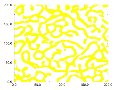
(a) $t=\tau_{S}$

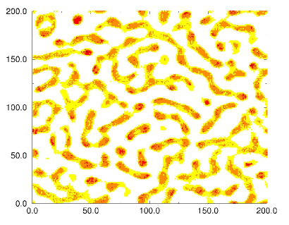
(b) $t=3\tau_{S}$

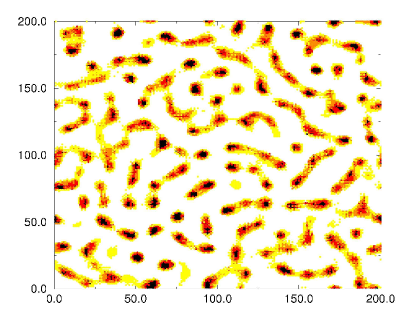
(c) $t=4\tau_{S}$

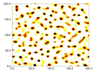
(d) $t=5\tau_{S}$

Figure 1: 2D growth of energy density perturbations for $\lambda=0.14$ and $g=1$ on a 200 $\times$ 200 lattice. Black areas correspond to $\rho>4\overline{\rho}$.

In Figure 2, we show the amplitude of the $S$ field at the centre of one of the energy density lumps in Figure 1. The oscillations of an unperturbed homogeneous inflaton field are shown for comparison. The field inside the lump is oscillating in time, showing that the inflaton condensate lump is indeed a quasi-stable oscillon. This is important, as it is not obvious that the energy density lumps in Figure 1 are not simply concentrations of the energy density with no coherent structure. If this were true, it would be possible for such concentrations to have a short lifetime due to a large amount of kinetic energy associated with their constituent scalar particles. The fact the energy density lumps are oscillons suggests that they will have a very long lifetime compared with the coherent oscillation period, as observed in numerical and analytical studies of single-field oscillons [13, 15].

Figure 2: Coherent oscillations of an energy density lump.

In Figure 3 we show the results of a 3-D simulation on a $50^{3}$ lattice. The regions where the energy density is greater than $4\overline{\rho}$ are shown. This clearly demonstrates the formation of inflaton condensate lumps in the 3-D case, confirming the results of the higher resolution 2-D simulations.

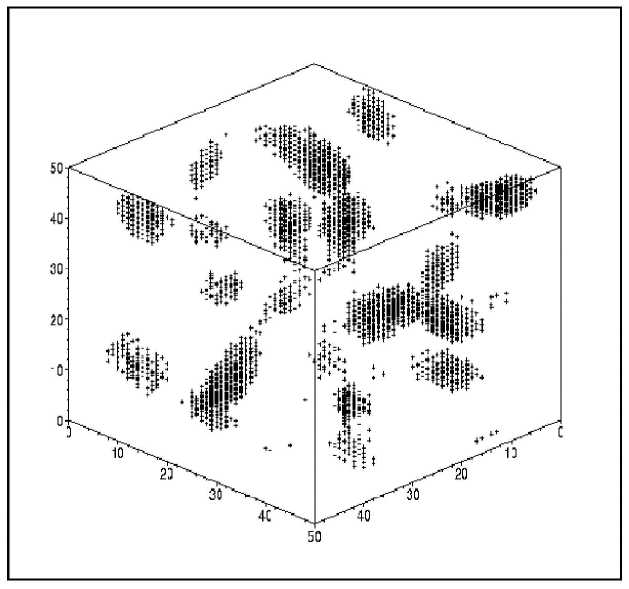
Figure 3: $50^{3}$ lattice 3D simulation. The plot shows regions of energy $\rho>4\overline{\rho}$ at $t=5\tau_{S}$.

We find no evidence of cosmic strings forming within the volume of our our lattice. This is consistent with our previous semi-analytical analysis, which indicated that the typical seperation of $U(1)_{FI}$ cosmic strings formed at the end of hybrid inflation would be not very much smaller than the horizon, corresponding to the wavelength of the first $\Phi_{-}$ fluctuations to be able to grow classically and break the $U(1)_{FI}$ symmetry [10].

5 A Scaling Property of the D-term Inflation Field Equations.

Throughout we have considered the case $g=1$. However, by rescaling the spacetime coordinates, the D-term inflation field equations can be written in a form that depends only upon the ratio $\lambda/g$. As a result, the condition for the formation of inflaton condensate lumps is likely to depend primarily upon the ratio $\lambda/g$, with only a weak logarithmic dependence on $g$ due to the initial value of the perturbations.

Under the rescaling of the coordinates $t=\tilde{t}/g$, $x=\tilde{x}/g$, the tree-level scalar field equations become

$$\mbox{$$}\ddot{S}+3\tilde{H}\dot{S}-\frac{{\bf\nabla}^{2}}{a^{2}}S=-\frac{\lambda^{2}}{g^{2}}|\Phi_{-}|^{2}S~{},\vspace{\undereqskip}$$ (12)

and

$$\mbox{$$}\ddot{\Phi}_{-}+3\tilde{H}\dot{\Phi}_{-}-\frac{{\bf\nabla}^{2}}{a^{2}}\Phi_{-}=-\frac{\lambda^{2}}{g^{2}}|S|^{2}\Phi_{-}+\left(\xi-|\Phi_{-}|^{2}\right)\Phi_{-}~{},\vspace{\undereqskip}$$ (13)

where derivatives are now with respect to $\tilde{x}$ and $\tilde{t}$. We have defined $\tilde{H}=a^{-1}da/d\tilde{t}=H/g$. $\tilde{H}$ is a function purely of $\lambda/g$. This follows since $H^{2}\propto\rho$ where, in terms of derivatives with respect to rescaled spacetime coordinates,

$$\mbox{$$}\rho=g^{2}\left(|\dot{S}|^{2}+|\dot{\Phi}_{-}|^{2}+\left|\frac{\nabla S}{a}\right|^{2}+\left|\frac{\nabla\Phi_{-}}{a}\right|^{2}+V(S,\Phi_{-})/g^{2}\right)\equiv g^{2}\tilde{\rho}~{}.\vspace{\undereqskip}$$ (14)

$V(S,\Phi_{-})/g^{2}$ is purely a function of $\lambda/g$, therefore $\tilde{\rho}$ depends only on $\lambda/g$. Thus $H\propto\rho^{1/2}=g\tilde{\rho}^{1/2}$ and so $\tilde{H}=H/g\propto\tilde{\rho}^{1/2}$. Therefore $\tilde{H}=\tilde{H}(\lambda/g)$.

The dependence of the rescaled field equations only on $\lambda/g$ does not extend to the quantum fluctuation initial conditions, Eq. (11). In terms of rescaled coordiantes and the rescaled wavenumber, $\tilde{k}=k/g$, the initial fluctuation becomes

$$\mbox{$$}\delta\phi(\tilde{{\bf x}},0)=\frac{1}{\sqrt{V}}\sum\frac{8g^{-1/2}}{\sqrt{2\tilde{k}_{\alpha\beta\gamma}}}\cos\left(\Delta\tilde{k}\Delta\tilde{x}\alpha i+\theta_{\alpha}\right)\cos\left(\Delta\tilde{k}\Delta\tilde{x}\beta j+\theta_{\beta}\right)\cos\left(\Delta\tilde{k}\Delta\tilde{x}\gamma k+\theta_{\gamma}\right)~{}.\vspace{\undereqskip}$$ (15)

The upper limit of the sum, corresponding to the largest value of $\tilde{k}$ for which the modes can grow, is determined from the rescaled field equations and is therefore purely a function of $\lambda/g$. Thus the initial conditions for the rescaled field equations are proportional to $g^{-1/2}$. However, the growth of perturbations in a tachyonic potential is typically rapid (exponential), in which case the condition for perturbations to become non-linear will depend only weakly (logarithmically) on the initial perturbation. As a result, if inflaton condensate lumps form for one value of $g$ (we considered $g=1$ in our simulations) then they will form for any value of $g$ for the same value of $\lambda/g$, up to a weak dependence on the initial conditions. The effect of reducing $g$ will be to increase the time for the lumps to form ($t=\tilde{t}/g$) and to increase the size of the resulting lumps ($x=\tilde{x}/g$).

6 Comparison with Previous Simulations

In [7] a simulation of SUSY hybrid inflation was reported for the case equivalent to D-term inflation couplings $\lambda=0.014$ and $g=0.14$, such that $\lambda/g=0.1$. It was concluded that the energy density would be transferred to inhomogeneous classical scalar field waves. Although no non-topological soliton formation was observed, this value of $\lambda/g$ is on the borderline of values for which we would expect to find non-topological soliton formation [10]. Therefore the results of [7] are not in any obvious way inconsistent with the results we have obtained here.

In [14] a simulation of the end of D-term was performed, again for the case equivalent to $\lambda=0.014$, $g=0.14$ in D-term inflation. The formation of non-topological solitons was observed along the length of cosmic strings. However, only quantum fluctuations of the symmetry-breaking field were considered in [14], with no inflaton fluctuations, which cannot be considered fully realistic. As discussed above, we expect that fluctuations of the symmetry-breaking field will only play a minor role in the evolution of the total energy density, being primarily associated with cosmic-string formation on scales not very much smaller than the horizon [10]. Nevertheless, the results in [14] confirm the possibility of non-topological soliton formation at the end of SUSY hybrid inflation.

7 Conclusions and Discussion

Our numerical simulations have shown that growth of quantum fluctuations of the scalar fields in SUSY hybrid inflation models results in the formation of inflaton condensate lumps corresponding to spherical lumps of coherently oscillating scalar field, also known as oscillons. The energy density of the Universe becomes almost entirely concentrated in these condensate lumps. We have focused on the case of D-term hybrid inflation, in which case the inflaton condensate lumps form if $\lambda\;^{>}_{\sim}\;0.1g$. Although a full analysis remain to be done, similar results may be expected in the case of F-term inflation, whose classical field equations are similar to those of D-term inflation for the case $\lambda=\sqrt{2}g$.

We have performed simulations for the case of a real inflaton field. The fact that the objects which form in this case are oscillons is significant, since from numerical and analytical studies of single-field oscillons such objects are known to be quasi-stable, with very long lifetimes compared to the scalar field coherent oscillation period. Therefore we expect that the post-inflation era will consist entirely of long-lived inflaton condensate lumps, even though our present numerical simulations are unable to resolve the evolution over more than about 10 coherent oscillation periods.

In the case of a complex inflaton field, oscillons are expected to be a precursor to stable Q-ball formation via decay to Q-ball pairs. Decay to Q-ball pairs is likely to occur long before the neutral inflaton condensate lumps decay via radiation of scalar field waves. Thus if inflaton condensate lumps form in the case of a real inflaton field, it is very likely that decay to Q-ball pairs and a Q-ball dominated post-inflation era will occur once a complex inflaton is considered. Since the Q-balls are classically stable, this era will only end once the scalar particles forming the Q-ball decay perturbatively to MSSM particles, reheating the Universe. A highly inhomogeneous inflaton condensate lump or Q-ball dominated era would have significant consequences for post-inflation SUSY cosmology. For example, it has been shown that the dynamics of scalar fields in the post-inflation era will not be subject to order $H$ mass corrections [20], with important consequences for Affleck-Dine baryogenesis, SUSY curvatons and moduli dynamics. Reheating will also be inhomogeneous, via Q-ball decay.

We plan to develop the capabilities of our numerical simulations in the future, with the ultimate goal of achieving a complete understanding of the post-inflation era of SUSY hybrid inflation models.

Appendix. Non-linear Growth of Quantum Fluctuations and the Equivalent Classical Stochastic Field

In this Appendix we review the growth of quantum fluctuations in the presence of a time-dependent tachyonic mass squared term. We first consider a real scalar field in Minkowski space with a positive or negative mass squared term. We then generalise to the case of a Friedmann-Robertson-Walker background, in particular de Sitter space.

In order to derive the classical initial conditions used in the lattice simulations, we quantize the theory in a box of side $L$. We consider an initial state corresponding to a Minkowski or Bunch-Davies vacuum state for a massive scalar field. The scalar field theory is exactly quantized in terms of creation and annihilation operators for momentum modes, which is valid so long as interaction terms can be neglected in the Hamiltonian, or equivalently the scalar field equations are linear. To follow the evolution of the quantum fluctuations into the non-linear regime, the quantum field theory is replaced by an equivalent classical field theory with a classical probability distribution for the initial conditions [21, 19], equivalent in the sense that the results of quantum field theory for the expectation values of products of fields are equal to the values obtained by solving the classical field equations with the classical probability distribution for the initial field values. This can be done if the occupation numbers of the quantum modes become large compared with one during the linear regime. The classical probability distribution is then given by the Wigner function of the field modes in the semi-classical limit. Although the classical probability distribution must become valid at some time during the period when the theory can be considered linear, once it becomes established it can be applied at any earlier time during the linear regime.

The Lagrangian and Hamiltonian for the scalar field in Minkowski space are

$$\mbox{$$}{\cal L}=\frac{1}{2}\partial_{\mu}\phi\partial^{\mu}\phi-\frac{m^{2}}{2}\phi^{2}~{},\vspace{\undereqskip}$$ (A-1)

and

$$\mbox{$$}{\cal H}=\pi\dot{\phi}-{\cal L}=\frac{1}{2}\left[\pi^{2}+({\bf\nabla}\phi)^{2}+m^{2}\phi^{2}\right]~{},\vspace{\undereqskip}$$ (A-2)

where the canonical momentum is $\pi\equiv\partial{\cal L}/\partial\dot{\phi}=\dot{\phi}$. We consider the scalar field in a cube of volume $L^{3}$ with periodic boundary conditions. The field and canonical momentum are expanded in terms of momentum modes as

$$\mbox{$$}\phi({\bf x},t)=\frac{1}{\sqrt{V}}\sum_{{\bf k}}q({\bf k},t)e^{i{\bf k}.{\bf x}}~{}\vspace{\undereqskip}$$ (A-3)

and

$$\mbox{$$}\pi({\bf x},t)=\frac{1}{\sqrt{V}}\sum_{{\bf k}}p({\bf k},t)e^{i{\bf k}.{\bf x}}~{},\vspace{\undereqskip}$$ (A-4)

where the components of ${\bf k}$ satisfy $k_{i}=2\pi n_{i}/L$ with $n_{i}$ an integer. $\pi({\bf x},t)=\dot{\phi}({\bf x},t)$ implies that $p({\bf k},t)=\dot{q}\left({\bf k},t\right)$. The non-zero equal-time canonical commutation relations for the field operators are

$$\mbox{$$}[\pi({\bf x},t),\phi({\bf x}^{{}^{\prime}},t)]=-i\delta^{3}\left({\bf x}-{\bf x}^{{}^{\prime}}\right)~{}.\vspace{\undereqskip}$$ (A-5)

The field and conjugate momentum mode operators must then satisfy

$$\mbox{$$}\left[p(-{\bf k},t),q({\bf l},t)\right]=-i\delta_{{\bf k},{\bf l}}~{}.\vspace{\undereqskip}$$ (A-6)

In terms of mode operators the Hamiltonian becomes

$$\mbox{$$}H=\frac{1}{2}\sum_{{\bf k}}p^{\dagger}({\bf k},t)p({\bf k},t)+\omega_{{\bf k}}^{2}q^{\dagger}({\bf k},t)q({\bf k},t)\;\;,\;\;\;\omega_{{\bf k}}^{2}={\bf k}^{2}+m^{2}~{},\vspace{\undereqskip}$$ (A-7)

where the mode operators satisfy the classical Hamiltonian equations of motion. In general, a Hamiltonian which is quadratic in the mode operators may be exactly quantized by expanding the operators in terms of time-independent creation and annihilation operators

$$\mbox{$$}q({\bf k},t)=f_{{\bf k}}a_{{\bf k}}+f_{{\bf k}}^{\dagger}a_{-{\bf k}}^{\dagger}~{}\vspace{\undereqskip}$$ (A-8)

and

$$\mbox{$$}p({\bf k},t)=-ig_{{\bf k}}a_{{\bf k}}+ig_{{\bf k}}^{\dagger}a_{-{\bf k}}^{\dagger}~{}\vspace{\undereqskip}$$ (A-9)

where $[a_{{\bf k}},a_{{\bf l}}^{\dagger}]=\delta_{{\bf k},{\bf l}}$. $p({\bf k},t)=\dot{q}({\bf k},t)$ implies that $g_{{\bf k}}=i\dot{f}_{{\bf k}}$. The mode functions $f_{{\bf k}}$ and $g_{{\bf k}}$ satisfy the classical field equations for the momentum modes (which are, by assumption, linear in $f_{{\bf k}}$) and the canonical commutation relations. The latter implies that the mode functions satisfy the condition $g_{{\bf k}}f_{{\bf k}}^{\dagger}+g_{{\bf k}}^{\dagger}f_{{\bf k}}=1$. For the case of a constant positive mass squared term, the mode functions $f_{{\bf k}}$ must also satisfy the condition that the Hamiltonian is correctly quantized, such that the energy eigenstates correspond to numbers of quanta of energy $\omega_{{\bf k}}$. The unique solution for $f_{{\bf k}}$ which satisfies both of these conditions is

$$\mbox{$$}f_{{\bf k}}=\frac{i}{\sqrt{2\omega_{{\bf k}}}}e^{-i\omega_{{\bf k}}t}~{}.\vspace{\undereqskip}$$ (A-10)

To study the evolution of the mode functions from an initial time $t=0$ at which $m^{2}\geq 0$, we use Eq. (A-10) as the initial condition for the mode functions. The subsequent evolution may then be studied by solving the classical equation of motion for $f_{{\bf k}}$ so long as we are in the linear regime, since in this case the field equations may be satisfied by field operators expanded in terms of time-independent creation and annihilation operators.

As an example, we consider the evolution for a model where a field is massless at $t\leq 0$ and gains a constant negative mass squared term once $t>0$. The field operator at $t>0$ satisfies the equation, for modes with $k^{2}<|m|^{2}$,

$$\mbox{$$}\ddot{q}\left({\bf k},t\right)=\tilde{\omega}_{{\bf k}}^{2}q\left({\bf k},t\right)\;,\;\;\;\tilde{\omega}^{2}_{{\bf k}}=|m|^{2}-{\bf k}^{2}~{},\vspace{\undereqskip}$$ (A-11)

with general solution

$$\mbox{$$}q({\bf k},t)=\alpha_{{\bf k}}e^{\tilde{\omega}_{{\bf k}}t}+\beta_{{\bf k}}e^{-\tilde{\omega}_{{\bf k}}t}~{}\vspace{\undereqskip}$$ (A-12)

and

$$\mbox{$$}p({\bf k},t)\equiv\dot{q}({\bf k},t)=\tilde{\omega}_{{\bf k}}\left(\alpha_{{\bf k}}e^{\tilde{\omega}_{{\bf k}}t}-\beta_{{\bf k}}e^{-\tilde{\omega}_{{\bf k}}t}\right)~{},\vspace{\undereqskip}$$ (A-13)

where $\alpha_{{\bf k}}$ and $\beta_{{\bf k}}$ are time-independent operators corresponding to linear combinations of $a_{{\bf k}}$ and $a_{-{\bf k}}^{\dagger}$. Matching these with the vacuum ($m=0$) solution at $t=0$ implies that

$$\mbox{$$}\alpha_{{\bf k}}=\frac{i}{2\sqrt{2\omega_{{\bf k}}}}\left[\left(1-\frac{i\omega_{{\bf k}}}{\tilde{\omega}_{{\bf k}}}\right)a_{{\bf k}}-\left(1+\frac{i\omega_{{\bf k}}}{\tilde{\omega}_{{\bf k}}}\right)a_{-{\bf k}}^{\dagger}\right]~{}\vspace{\undereqskip}$$ (A-14)

and

$$\mbox{$$}\beta_{{\bf k}}=\frac{i}{2\sqrt{2\omega_{{\bf k}}}}\left[\left(1+\frac{i\omega_{{\bf k}}}{\tilde{\omega}_{{\bf k}}}\right)a_{{\bf k}}-\left(1-\frac{i\omega_{{\bf k}}}{\tilde{\omega}_{{\bf k}}}\right)a_{-{\bf k}}^{\dagger}\right]~{},\vspace{\undereqskip}$$ (A-15)

where $\omega_{{\bf k}}=|{\bf k}|$. Therefore $q({\bf k},t)$ for $t>0$ can be written in the form of Eq. (A-8) with

$$\mbox{$$}f_{{\bf k}}=\frac{i}{2\sqrt{2\omega_{{\bf k}}}}\left[\left(1-\frac{i\omega_{{\bf k}}}{\tilde{\omega}_{{\bf k}}}\right)e^{\tilde{\omega}_{{\bf k}}t}+\left(1+\frac{i\omega_{{\bf k}}}{\tilde{\omega}_{{\bf k}}}\right)e^{-\tilde{\omega}_{{\bf k}}t}\right]~{}.\vspace{\undereqskip}$$ (A-16)

For $\tilde{\omega}_{{\bf k}}t\gg 1$, $q({\bf k},t)\approx\alpha_{{\bf k}}e^{\tilde{\omega}_{{\bf k}}t}$ and $p({\bf k},t)\approx\omega_{{\bf k}}\alpha_{{\bf k}}e^{\tilde{\omega}_{{\bf k}}t}$, so that to a good approximation $q({\bf k},t)$ and $p({\bf k},t)$ commute, corresponding to the limit of classical physics.

In order to study the growth of quantum fluctuations beyond the linear regime, we need the classical stochastic initial conditions which reproduce the field theory expectation values in the semi-classical limit. The classical probability distribution is obtained from the Wigner function,

$$\mbox{$$}W(q,p,t)=\int\frac{dx_{1}dx_{2}}{\left(2\pi\right)^{2}}e^{-i\left(p_{1}x_{1}+p_{2}x_{2}\right)}<q-\frac{x}{2},t|\rho|q+\frac{x}{2},t>~{},\vspace{\undereqskip}$$ (A-17)

where $p=p_{1}+ip_{2}$, $q=q_{1}+iq_{2}$ and $x=x_{1}+ix_{2}$. The $q$ and $p$ represent complex generalised coordinates and conjugate momenta, which in our case correspond to $q({\bf k},t)$ and $p({\bf k},t)$. $\rho=|\psi_{o}(t)><\psi_{o}(t)|$ is the density matrix of the Schrodinger picture state, $|\psi_{o}(t)>$, which evolves from the initial vacuum state. In general the Wigner function gives the probability distribution of the observable $q$ at $t$ after integrating over $p$ and vice-versa. In the classical limit the Wigner function tends towards a classical probability distribution, $f(q,p,t)$, which reproduces the quantum field theory results for expectation values of the field operators. Although $f(q,p,t)$ should be calculated in the semi-classical limit, it can be applied at any time during the linear evolution of the field, in particular at earlier times, since it satisfies the classical equations of motion [21]. In the case of hybrid inflation we can therefore apply the classical initial conditions at the end of inflation ($s=s_{c}$), corresponding to massless scalar fields.

The annihilation operators can be expressed as

$$\mbox{$$}a_{{\bf k}}=\frac{g_{{\bf k}}^{\dagger}}{2Re(f_{{\bf k}}g_{{\bf k}}^{\dagger})}\left(q({\bf k},t)-\frac{f_{{\bf k}}^{\dagger}}{ig_{{\bf k}}^{\dagger}}p({\bf k},t)\right)~{}.\vspace{\undereqskip}$$ (A-18)

By definition $a_{{\bf k}}|0>=0$, where the Heisenberg picture initial vacuum state, $|0>$, is equivalent to the Schrodinger picture vacuum state at $t=0$. In order to obtain the Schrodinger wavefunction $\psi(q,t)\equiv<q|\psi_{o}(t)>$ corresponding to the state evolving from the initial vacuum state, we express the equation $a_{{\bf k}}|0>$ as a wave equation in the position representation [19]. In terms of the time evolution operator $U(t)$, $a_{{\bf k}}|0>=0$ can be expressed as

$$\mbox{$$}U^{\dagger}[q({\bf k},0)+\frac{if_{k}^{\dagger}}{g_{k}^{\dagger}}p({\bf k},0)]U|0>=0~{},\vspace{\undereqskip}$$ (A-19)

where $q({\bf k},t)=U^{\dagger}q({\bf k},0)U$. Since $U|0>\equiv|\psi_{o}(t)>$ is the time-dependent Schrodinger state vector and $q({\bf k},0)\equiv q_{{\bf k}}$ , $p({\bf k},0)\equiv p_{{\bf k}}$ are the Schrodinger representation generalised coordinate and momentum operators, with $p_{{\bf k}}$ conjugate to $q_{-{\bf k}}\equiv q^{\dagger}_{{\bf k}}$ ($[p_{{\bf k}},q_{{\bf k}}^{\dagger}]=-i$), the momentum operator in the position representation becomes $p_{{\bf k}}=-i\partial/\partial q_{{\bf k}}^{*}$. The wave equation can then be written as

$$\mbox{$$}\left(q_{{\bf k}}+\frac{f_{{\bf k}}^{\dagger}}{g_{{\bf k}}^{\dagger}}\frac{\partial}{\partial q_{{\bf k}}^{*}}\right)\psi_{o}\left(q_{{\bf k}},q_{{\bf k}}^{*},t\right)=0~{}.\vspace{\undereqskip}$$ (A-20)

This has the solution [19]

$$\mbox{$$}\psi_{o}(q_{{\bf k}},q_{{\bf k}}^{*},t)=N_{o}\exp\left(-\frac{g_{k}^{\dagger}}{f_{k}^{\dagger}}|q_{{\bf k}}|^{2}\right)~{},\vspace{\undereqskip}$$ (A-21)

where $N_{o}=(\sqrt{\pi}|f_{{\bf k}}|)^{-1}$. The normalized probability distribution is then

$$\mbox{$$}P(q_{{\bf k}},q_{{\bf k}}^{*},t)=\frac{1}{\pi|f_{{\bf k}}|^{2}}exp\left(-\frac{|q_{{\bf k}}|^{2}}{|f_{{\bf k}}(t)|^{2}}\right)~{}.\vspace{\undereqskip}$$ (A-22)

This gives the probability that the magnitude of the classical mode amplitude $q({\bf k},t)$ at $t$ is $|q_{{\bf k}}|$. This is a complex Gaussian distribution, with r.m.s. value for $|q_{{\bf k}}|$ equal to $|f_{{\bf k}}|$. Then $q({\bf k},t)=|q({\bf k},t)|e^{i\delta_{{\bf k}}}$, with $\delta_{{\bf k}}$ a random phase.

The Wigner function is then given by

$$\mbox{$$}W(q_{{\bf k}},p_{{\bf k}},t)=\int\int\frac{dx_{1}dx_{2}}{\left(2\pi\right)^{2}}e^{-i\left(p_{{\bf k}\;1}x_{1}+p_{{\bf k}\;2}x_{2}\right)}\psi_{o}^{*}(q_{{\bf k}}-x/2,t)\psi_{o}(q_{{\bf k}}+x/2,t)~{}.\vspace{\undereqskip}$$ (A-23)

Integrating gives

$$\mbox{$$}W(q_{{\bf k}},p_{{\bf k}},t)=\frac{1}{\pi^{2}}\exp\left[-\frac{|q_{{\bf k}}|^{2}}{|f_{{\bf k}}|^{2}}-|f_{{\bf k}}|^{2}\left|p_{{\bf k}}-\frac{F_{{\bf k}}}{|f_{{\bf k}}|^{2}}q_{{\bf k}}\right|^{2}\right]~{},\vspace{\undereqskip}$$ (A-24)

where $F_{{\bf k}}=Im(f_{{\bf k}}^{\dagger}g_{{\bf k}})$. In the limit $|f_{{\bf k}}|^{2}\gg 1$, where the Wigner function tends towards the classical probability distribution, the Wigner function is vanishing except if

$$\mbox{$$}p_{{\bf k}}=\frac{F_{{\bf k}}}{|f_{{\bf k}}|^{2}}q_{{\bf k}}~{}.\vspace{\undereqskip}$$ (A-25)

Since the classical probability distribution can be applied at any time during the linear regime, we can choose to apply the initial conditions at the end of hybrid inflation, such that the fields are massless. For the case of flat space, the mode functions with $m=0$ are given by

$$\mbox{$$}f_{{\bf k}}=\frac{i}{\sqrt{2k}}e^{-ikt}\;,\;\;\;g_{{\bf k}}=i\sqrt{\frac{k}{2}}e^{-ikt}~{},\vspace{\undereqskip}$$ (A-26)

where $k=|{\bf k}|$. Thus $F_{{\bf k}}=Im(f_{{\bf k}}^{\dagger}g_{{\bf k}})=0$. Therefore the flat space classical initial condition for $p({\bf k},t)$ is $p({\bf k},0)=0$, whilst the flat space classical initial conditions for $q({\bf k},t)$ at $t=0$ corresponds to a complex Gaussian distribution for $|q({\bf k},0)|$, with r.m.s. value

$$\mbox{$$}|q({\bf k},0)|_{rms}=\frac{1}{\sqrt{2k}}~{}\vspace{\undereqskip}$$ (A-27)

and with a random phase factor $e^{i\delta_{{\bf k}}}$ for each ${\bf k}$.

These results can easily be generalised to a scalar field in Friedman-Robertson-Walker spacetime. In this case the action is

$$\mbox{$$}S=\int d^{4}x\sqrt{-g}\left[\frac{1}{2}\partial_{\mu}\phi\partial^{\mu}\phi-\frac{m^{2}}{2}\phi^{2}\right]~{}.\vspace{\undereqskip}$$ (A-28)

In terms of $y=a(t)\phi$ and conformal time $\eta$ ($dt=a(t)d\eta$), where $a(t)$ is the scale factor, this becomes

$$\mbox{$$}S=\int d^{4}x\left[\frac{1}{2}\left(y^{{}^{\prime}}-\frac{a^{{}^{\prime}}}{a}y\right)^{2}-\frac{\left(\nabla y\right)^{2}}{2}-\frac{m^{2}a^{2}}{2}y^{2}\right]~{},\vspace{\undereqskip}$$ (A-29)

where ^′ denotes differentiation with respect to conformal time and $d^{4}x$ is now understood as an integral over comoving coordinates and conformal time. The conjugate momentum is

$$\mbox{$$}\pi=\frac{\partial{\cal L}}{\partial y^{{}^{\prime}}}=y^{{}^{\prime}}-\frac{a^{{}^{\prime}}}{a}y~{}\vspace{\undereqskip}$$ (A-30)

and the Hamiltonian is

$$\mbox{$$}H=\int d^{3}x\left[\frac{\pi^{2}}{2}+\frac{\left(\nabla y\right)^{2}}{2}+\frac{m^{2}a^{2}}{2}y^{2}+\frac{a^{{}^{\prime}}}{a}\pi y\right]~{}.\vspace{\undereqskip}$$ (A-31)

Expanding $y({\bf x},\eta)$ and $\pi({\bf x},\eta)$ in terms of modes as before (but now with $\eta$ in place of $t$ and $y$ in place of $\phi$) implies that

$$\mbox{$$}H=\frac{1}{2}\sum_{{\bf k}}\left[p({\bf k},\eta)^{\dagger}p({\bf k},\eta)+\omega_{{\bf k}}^{2}q({\bf k},\eta)^{\dagger}q({\bf k},\eta)+\frac{a^{{}^{\prime}}}{a}\left(p({\bf k},\eta)q^{\dagger}({\bf k},\eta)+p^{\dagger}({\bf k},\eta)q({\bf k},\eta)\right)\right]~{},\vspace{\undereqskip}$$ (A-32)

where $\omega_{{\bf k}}^{2}={\bf k}^{2}+m^{2}a^{2}$ and

$$\mbox{$$}p({\bf k},\eta)=q^{{}^{\prime}}({\bf k},\eta)-\frac{a^{{}^{\prime}}}{a}q({\bf k},\eta)~{}.\vspace{\undereqskip}$$ (A-33)

This is quantized by expanding $q$ and $p$ in terms of creation and annihilation operators according to Eq. (A-8) and Eq. (A-9). The mode functions satisfy the classical equation of motion

$$\mbox{$$}f_{{\bf k}}^{{}^{\prime\prime}}-\frac{a^{{}^{\prime\prime}}}{a}f_{{\bf k}}=-\left({\bf k}^{2}+m^{2}a^{2}\right)f_{{\bf k}}~{},\vspace{\undereqskip}$$ (A-34)

with the requirement that the initial $f_{{\bf k}}$ reduces to the Minkowski modes in the limit $k\gg H$ (Bunch-Davies vacuum).

For the case of de Sitter space, $H=constant$, the mode equation becomes

$$\mbox{$$}f_{{\bf k}}^{{}^{\prime\prime}}+\left[k^{2}-\frac{\left(2-\frac{m^{2}}{H^{2}}\right)}{\eta^{2}}\right]f_{{\bf k}}=0~{},\vspace{\undereqskip}$$ (A-35)

where $\eta=-1/aH$. For a constant $m^{2}$, the solution which tends to the Minkowski vacuum in the limit $k\gg H$ is

$$\mbox{$$}f_{{\bf k}}(\eta)=\frac{\sqrt{\pi}}{2}e^{i\left(\frac{\pi}{2}\nu+\frac{\pi}{4}\right)}\sqrt{-\eta}H_{\nu}^{(1)}\left(-k\eta\right)\;,\;\;\;\nu^{2}=\frac{9}{4}-\frac{m^{2}}{H^{2}}~{},\vspace{\undereqskip}$$ (A-36)

where $H^{(1)}_{\nu}$ is a spherical Hankel function of the first kind.

The Wigner function analysis is as before except with $\eta$ in place of $t$. $f_{{\bf k}}$ is now given by Eq. (A-36), whilst $g_{{\bf k}}$ follows from $p({\bf k},\eta)=q^{{}^{\prime}}({\bf k},\eta)-(a^{{}^{\prime}}/a)q({\bf k},\eta)$, which implies that $g_{{\bf k}}=i(f_{{\bf k}}^{{}^{\prime}}-(a^{{}^{\prime}}/a)f_{{\bf k}})$. The initial conditions we impose correspond to de Sitter space with a massless field, in which case $\nu=3/2$ and so

$$\mbox{$$}f_{{\bf k}}=\frac{i\sqrt{\pi}}{2}\sqrt{-\eta}H_{\frac{3}{2}}^{(1)}\left(-k\eta\right)=\frac{e^{-ik\eta}}{\sqrt{2k}}\left[1-\frac{i}{k\eta}\right]~{}\vspace{\undereqskip}$$ (A-37)

$$\mbox{$$}g_{{\bf k}}=\sqrt{\frac{k}{2}}e^{-ik\eta}~{},\vspace{\undereqskip}$$ (A-38)

where we have used the expression for the Hankel function,

$$\mbox{$$}H_{3/2}^{\left(1\right)}(x)=-\left(\frac{2}{\pi x}\right)^{1/2}e^{ix}\left[1+\frac{i}{x}\right]~{}.\vspace{\undereqskip}$$ (A-39)

Thus $F_{{\bf k}}=Im(f_{{\bf k}}^{\dagger}g_{{\bf k}})=1/(2k\eta)$. The classical r.m.s. values for the magnitudes of the mode functions are then

$$\mbox{$$}|q({\bf k},\eta)|_{rms}=|f_{{\bf k}}|=\frac{1}{\sqrt{2k}}\left(1+\frac{1}{k^{2}\eta^{2}}\right)^{1/2}~{}\vspace{\undereqskip}$$ (A-40)

and

$$\mbox{$$}|p({\bf k},\eta)|_{rms}=\frac{1}{\sqrt{2k}|\eta|}\left(1+\frac{1}{k^{2}\eta^{2}}\right)^{-1/2}~{}.\vspace{\undereqskip}$$ (A-41)

These may be used to model the initial conditions for the massless scalar fields at the end of hybrid inflation.

In practice, we numerically solve the classical scalar field equations for $\phi({\bf x},t)$ rather than $y({\bf x},\eta)$. In general, $y({\bf x},\eta)=a\phi({\bf x},t)$ and $\pi({\bf x},\eta)=a^{2}\dot{\phi}({\bf x},t)$. Choosing $a=1$ at the end of inflation (corresponding to choosing $\eta=-H^{-1}$ at $t=0$) implies that $\phi({\bf x},0)=y({\bf x},\eta)$ and $\dot{\phi}({\bf x},0)=\pi({\bf x},\eta)$ at the end of inflation. In this case the mode functions in Eq. (A-40) and Eq. (A-41) will provide the initial conditions for the mode expansions of $\phi({\bf x},t)$ and $\dot{\phi}({\bf x},t)$ in de Sitter space.

References

- [1]
- [2] A.Linde, Phys. Rev. D49 (1994) 748.
- [3] E.Halyo, Phys. Lett. B387 (1996) 43; P.Binetruy and G.Dvali, Phys. Lett. B388 (1996) 241.
- [4] G.Dvali, Q.Shafi and R.Schafer, Phys. Rev. Lett. 73 (1994) 1886; E.J.Copeland, A.R.Liddle, D.H.Lyth, E.D.Stewart and D.Wands, Phys. Rev. D49 (1994) 6410.
- [5] D.Lyth and A.Riotto, Phys. Rep. 314 (1999) 1.
- [6] N.Arkani-Hamed and S.Dimopoulos, hep-th/0405159; G.F.Giudice and A.Romanino, Nucl. Phys. B699 (2004) 65; N.Arkani-Hamed, S.Dimopoulos, G.F.Giudice and A.Romanino, Nucl. Phys. B709 (2005) 3.
- [7] G.Felder, J.Garcia-Bellido, P.B.Greene, L.Kofman, A.Linde and I.Tkachev, Phys. Rev. Lett. 87 (2001) 011601.
- [8] G.Felder, L.Kofman and A.Linde, Phys. Rev. D64 (2001) 123517.
- [9] J.McDonald, Phys. Rev. D66 (2002) 043525.
- [10] M.Broadhead and J.McDonald, Phys. Rev. D68 (2003) 083502.
- [11] G.Felder and L.Kofman, Phys. Rev. D70 (2004) 046004.
- [12] A.Arrizabalaga, J.Smit and A.Tranberg, JHEP 0410 (2004) 017; A.Tranberg and J.Smit, JHEP 0311 (2003) 016; J.Garcia-Bellido, M.G.Perez and A.Gonzalez-Arroyo, Phys. Rev. D67 (2003) 103501; J.Smit and A.Tranberg, JHEP 0212 (2002) 020.
- [13] M.Gleiser and A.Sornborger, Phys. Rev. E62 (2000) 1368; E.J.Copeland, M.Gleiser and H.R.Muller, Phys. Rev. D52 (1995) 1920; M. Gleiser, Phys. Rev. D49 (1994) 2978.
- [14] E.J.Copeland, S.Pascoli and A.Rajantie, Phys. Rev. D65 (2002) 103517.
- [15] S.Kasuya, M.Kawasaki and F.Takahashi, Phys. Lett. B559 (2003) 99.
- [16] M.Broadhead and J.McDonald, Phys. Rev. D69 (2004) 063510.
- [17] S.Kasuya and M.Kawasaki, Phys. Rev. D61 (2000) 041301; Phys. Rev. D62 (2000) 023512.
- [18] K.Enqvist, S.Kasuya and A.Mazumdar, Phys. Rev. D66 (2002) 043505.
- [19] D.Polarski and A.Starobinsky, Class. Quant. Grav. 13 (1996) 377.
- [20] J.McDonald, JCAP 0408 (2004) 002.
- [21] A.Guth and S.Y.Pi, Phys. Rev. D32 (1985) 1899.