QUINTESSENTIAL KINATION AND
COLD DARK MATTER ABUNDANCE

Abstract

The generation of a kination-dominated phase by a quintessential exponen-tial model is investigated and the parameters of the model are restricted so that a number of observational constraints (originating from nucleosynthesis, the present acceleration of the universe and the dark-energy-density parameter) are satisfied. The decoupling of a thermal cold dark matter particle during the period of kination is analyzed, the relic density is calculated both numerically and semi-analytically and the results are compared with each other. It is argued that the enhancement, with respect to the standard paradigm, of the cold dark matter abundance can be expressed as a function of the quintessential density parameter at the onset of nucleosynthesis. We find that values of the latter quantity close to its upper bound require the thermal-averaged cross section times the velocity of the cold relic to be almost three orders of magnitude larger than this needed in the standard scenario so as compatibility with the cold dark matter constraint is achieved.

Cosmology, Dark Energy, Dark Matter

J. Cosmol. Astropart. Phys. 015, 10 (2005)

 

1 INTRODUCTION

A plethora of recent data [1, 2] has indicated that the two major components of the present universe are the Cold (mainly [3]) Dark Matter (CDM) and the Dark Energy (DE) with density parameters [1], respectively:

$${\sf(a)}~{}~{}\Omega_{\rm CDM}=0.24\pm 0.1~{}~{}\mbox{and}~{}~{}{\sf(b)}~{}~{}\Omega_{\rm DE}=0.73\pm 0.12,$$ (1)

at $95\%$ confidence level (c.l.). The identification of these two unknown substances consists one of the most tantalizing enigmas of the modern cosmo-particle theories.

As regards CDM, the most natural candidates [4] are the weekly interacting massive particles, $\chi$’s. The most popular of these is the lightest supersymmetric (SUSY) particle (LSP) [5]. However, the extra dimensional (ED) theories give rise to new CDM candidates [6, 7, 8]. According to the standard cosmological scenario (SC) [9], $\chi$’s (i) are produced through thermal scatterings in the plasma, (ii) reach chemical equilibrium with plasma and (iii) decouple from the cosmic fluid during the radiation-dominated (RD) era (note that these assumptions are, also, naturally valid in the case of the so-called second Randall-Sundrum [10] model, provided that the brane-tension is constrained to rather high values [11]). The viability of other CDM candidates (like axions [12], axino [13], gravitino [14], quintessino [15]) requires a somehow different cosmological set-up, which we do not consider in our analysis. In light of eq. (1), the $\chi$-relic density, $\Omega_{\chi}h_{0}^{2}$, is to satisfy the following range of values:

$${\sf(a)}~{}~{}0.09\lesssim\Omega_{\chi}h_{0}^{2}~{}~{}\mbox{and}~{}~{}{\sf(b)}~{}~{}\Omega_{\chi}h_{0}^{2}\lesssim 0.13.$$ (2)

As regards DE, quintessence [16], a slowly evolving scalar field, has recently attracted much attention (for reviews, see ref. [17]). The scalar field is supposed to roll down its potential undergoing three phases during its cosmological evolution: Initially its kinetic energy, which decreases faster than the radiation, dominates and gives rise to a possible novel period in the universal history termed “kination” [18]. Then, the scalar field freezes to a value close to Planck scale and by now its potential energy, adjusted so that eq. (1b) is met, becomes dominant. Such an adjustment, which certainly does not resolve satisfactorily the coincidence problem, is unavoidable in quintessential models (for related suggestions, see refs. [19, 20]). Other shortcomings such as the lightness of the scalar field [21] or the time variation of the gauge coupling constants [22] are currently under investigation.

Be that as it may, the viability of a quintessential scenario can be controlled by imposing some observational constraints [23], arising from nucleosynthesis, acceleration of the universe and the DE density parameter. Unfortunately no full-satisfactory potential exists, to date (for comparative explorations of various potentials, see refs. [24, 25]). E.g., the inverse power potential [26] although provides a tracker-type solution [27] does not fit well [28] the present-day value [1, 2] of the quintessence-equation-of-state parameter. Phenomenologically more robust [25] is the supergravity-inspired [28, 29] potential without, however, to allow a zero minimum of the potential [28, 3]. Also, in both cases, the generation in the early universe of a kination-dominated (KD) expansion consistent with the fulfillment of the requirements above is rather questionable [30, 31]. For these reasons, we decide to examine the simplest exponential potential [32, 29], which, although does not possess a tracker-type solution [27, 30], it can produce a viable present-day cosmology in conjunction with the domination of an early KD era, for a reasonable region of initial conditions [23, 25, 33].

The departure from the SC, caused by the implementation of a quintessential KD epoch can modify the $\Omega_{\chi}h_{0}^{2}$ calculation, which (as, already, emphasized [34, 35, 36, 37]) crucially dependents on the adopted assumptions. If the quintessential KD phase dominates over the radiation (a condition indispensable for the quintessential inflationary model-building [38, 39, 40]), the assumption (iii) of the SC is lifted (note that the assumptions (i) and (ii) are maintained). As a consequence, an increase to $\Omega_{\chi}h_{0}^{2}$ with respect to (w.r.t) its value in the SC is implied. This phenomenon was first pointed out in ref. [30] and was explored in ref. [41] for the parameters of the exponential potential, which support a global attractor [42]. There [41], $\Omega_{\chi}h_{0}^{2}$ was calculated numerically for a couple of SUSY models which resurrect higgsino [43] or wino [44] LSP and can yield acceptable $\Omega_{\chi}h_{0}^{2}$.

Contrary to ref. [41], we focus on the range of the exponential-potential parameters, which ensures a late-time attractor together with an early KD regime (see sec. 2.2) and can lead to a simultaneous satisfaction of several observational data (see secs. 2.3 and 4.2). We then, present a “unified” (using the same independent variable) description of the cosmological evolution of the quintessence field and the $\chi$ decoupling (see secs. 2.2 and 3.3). The relevant equations are solved both numerically (see secs. 2.1 and 3.2) and semi-analytically (see secs. 2.2 and 3.3) and the results are compared with each other (see secs. 4.1 and 4.3). Finally, we demonstrate the crucial correlation between the $\Omega_{\chi}h_{0}^{2}$ enhancement (w.r.t the one in the SC) and the quintessential density parameter at the eve of nucleosynthesis (see sec. 4.3) and we restrict the parameters imposing all the DE and CDM constraints (see sec. 4.4) without, however, to adopt a specific particle model. We showed that values of the quintessential density parameter at the former point close to its upper bound require the thermal-averaged cross section times the velocity of $\chi$ to be almost three orders of magnitude larger than this needed in the SC.

The framework of the quintessential cosmology is described in sec. 2, while our numerical and semi-analytical $\Omega_{\chi}h_{0}^{2}$ calculations are displayed in sec. 3. Some numerical applications are presented in sec. 4. Finally, sec. 5 summarizes our results and discusses some open questions. Throughout the text and the formulas, brackets are used by applying disjunctive correspondence, natural units ($\hbar=c=k_{\rm B}=1$) are assumed, the subscript or superscript $0$ is referred to present-day values and $\ln~{}[\log]$ stands for logarithm with basis $e~{}[10]$.

2 QUINTESSENTIAL COSMOLOGY

We briefly describe the equations which govern the evolution of the universe in the presence of quintessence (sec. 2.1), the phases which the quintessence field undergoes during its evolution (sec. 2.2) and the requirements which a successful quintessential scenario is to satisfy (sec. 2.3).

2.1 RELEVANT EQUATIONS

According to the quintessential scenario, we assume the existence of a spatially homogeneous, scalar field $q$ (not to be confused with the deceleration parameter [3]) which obeys the Klein-Gordon equation. We below present its archetypal form and then we derive simplified forms which facilitate its numerical integration. Finally, we specify the used initial conditions and we define the useful extracted quantities.

2.1.1 Initial form.

The homogeneous Klein-Gordon equation in a cosmological set-up is

$$\mbox{\sf(a)}~{}~{}\ddot{q}+3H\dot{q}+V_{,q}=0,~{}~{}\mbox{where}~{}~{}\mbox{\sf(b)}~{}~{}V=V_{o}e^{-\lambda q/m_{{}_{\rm P}}}$$ (1)

is the adopted potential for the field $q$, $,q$ [dot] stands for derivative w.r.t $q$ [the cosmic time, $t$] and $H$ is the Hubble expansion parameter,

$$\mbox{\sf(a)}~{}~{}H=\sqrt{\rho_{q}+\rho_{{}_{\rm R}}+\rho_{{}_{\rm M}}}/\sqrt{3}m_{{}_{\rm P}}~{}~{}\mbox{with}~{}~{}\mbox{\sf(b)}~{}~{}\rho_{q}=\frac{1}{2}\dot{q}^{2}+V,$$ (2)

the energy density of $q$ and $m_{{}_{\rm P}}=M_{\rm P}/8\pi$, where $M_{\rm P}=1.22\times 10^{19}~{}{\rm GeV}$ is the Planck mass. The energy density of radiation, $\rho_{{}_{\rm R}}$, can be evaluated as a function of temperature, $T$, whilst the energy density of matter, $\rho_{{}_{\rm M}}$, with reference to its present-day value:

$$\mbox{\sf(a)}~{}~{}\rho_{{}_{\rm R}}=\frac{\pi^{2}}{30}g_{\rho*}\ T^{4}~{}~{}\mbox{and}~{}~{}\mbox{\sf(b)}~{}~{}\rho_{{}_{\rm M}}R^{3}=\rho^{0}_{{}_{\rm M}}R_{0}^{3}$$ (3)

with $R$, the scale factor of the universe. Assuming no entropy production caused by the domination of another field (entropy production due to the $q$ domination is not expected, since it does not couple to matter), the entropy density, $s$, satisfies the following two equations:

$$\mbox{\sf(a)}~{}~{}sR^{3}=s_{\rm p}R_{\rm p}^{3}~{}~{}\mbox{where}~{}~{}\mbox{\sf(b)}~{}~{}s=\frac{2\pi^{2}}{45}g_{s*}\ T^{3},$$ (4)

where subscript “p” represents a specific reference point at which the constant quantity $sR^{3}$ is evaluated and $g_{\rho*}(T)~{}[g_{s*}(T)]$ is the energy [entropy] effective number of degrees of freedom at temperature $T$. Their numerical values are evaluated by using the tables included in micrOMEGAs [45], originated from the DarkSUSY package [46] (recent improvements [47] do not affect essentially the results).

2.1.2 Reformulation.

The numerical integration of eq. (1) is facilitated by converting the time derivatives to derivatives w.r.t the logarithmic time [23, 25]:

$$\leavevmode\hbox{\normalsize$\tau$\kern-5.0pt$\iota$}=\ln\left(R/R_{0}\right)=-\ln(1+z)~{}~{}(\Rightarrow~{}\dot{\leavevmode\hbox{\normalsize$\tau$\kern-5.0pt$\iota$}}=H)$$ (5)

with $z$ the redshift. Changing the differentiation, eq. (1) turns out to be equivalent to the system of two first-order equations (prime denotes derivative w.r.t $\tau$$\iota$):

$$\mbox{\sf(a)}~{}~{}Q=Hq^{\prime}~{}~{}\mbox{and}~{}~{}\mbox{\sf(b)}~{}~{}HQ^{\prime}+3HQ+V_{,q}=0~{}~{}\mbox{with}~{}~{}\mbox{\sf(c)}~{}~{}\rho_{q}=\frac{1}{2}Q^{2}+V.$$ (6)

In terms of $\tau$$\iota$ in eq. (5), $s$ and $T$ can be expressed through the relations :

$$\mbox{\sf(a)}~{}~{}s=s_{0}e^{-3\leavevmode\hbox{\footnotesize$\tau$\kern-4.0pt$\iota$}}~{}~{}\mbox{and}~{}~{}\mbox{\sf(b)}~{}~{}T=T_{0}\left(\frac{g^{0}_{s*}}{g_{s*}}\right)^{1/3}e^{-{\leavevmode\hbox{\footnotesize$\tau$\kern-4.0pt$\iota$}}},$$ (7)

where eqs. (4a) and (4b) have been used. Similarly, $\rho_{{}_{\rm R}}$ and $\rho_{{}_{\rm M}}$ are elegantly cast in the form:

$$\mbox{\sf(a)}~{}~{}\rho_{{}_{\rm R}}=\rho^{0}_{{}_{\rm R}}\frac{g_{\rho*}}{g^{0}_{\rho*}}\left(\frac{g^{0}_{s*}}{g_{s*}}\right)^{4/3}e^{-4\leavevmode\hbox{\footnotesize$\tau$\kern-4.0pt$\iota$}}~{}~{}\mbox{and}~{}~{}\mbox{\sf(b)}~{}~{}\rho_{{}_{\rm M}}=\rho^{0}_{{}_{\rm M}}e^{-3\leavevmode\hbox{\footnotesize$\tau$\kern-4.0pt$\iota$}}.$$ (8)

Eq. (8a) was extracted by inserting eq. (7b) in eq. (3a). Eq. (8b) can be derived by combining eq. (5) with eq. (3b).

2.1.3 Normalized form.

An even more numerically “robust” [25] form of eq. (6) can be achieved, if we introduce the following dimensionless quantities:

$$\mbox{\sf(a)}~{}~{}{\mbox{$\bar{\rho}$}}_{{}_{\rm M[R]}}=\rho_{{}_{\rm M[R]}}/\rho^{0}_{\rm c},~{}~{}\mbox{\sf(b)}~{}~{}{\mbox{$\bar{V}_{o}$}}=V_{o}/\rho^{0}_{\rm c}~{}~{}\mbox{and}~{}~{}\mbox{\sf(c)}~{}~{}{\mbox{$\bar{q}$}}=q/\sqrt{3}m_{{}_{\rm P}}.$$ (9)

Employing these quantities, eq. (6) can be re-written as:

$$\mbox{\sf(a)}~{}~{}{\mbox{$\bar{Q}$}}={\mbox{$\bar{H}$}}{\mbox{$\bar{q}$}}^{\prime}~{}~{}\mbox{and}~{}~{}\mbox{\sf(b)}~{}~{}{\mbox{$\bar{H}$}}{\mbox{$\bar{Q}$}}^{\prime}+3{\mbox{$\bar{H}$}}{\mbox{$\bar{Q}$}}+\bar{V}_{,\bar{q}}=0~{}~{}\mbox{with}~{}~{}\mbox{\sf(c)}~{}~{}{\mbox{$\bar{H}$}}^{2}={\mbox{$\bar{\rho}$}}_{q}+{\mbox{$\bar{\rho}$}}_{{}_{\rm R}}+{\mbox{$\bar{\rho}$}}_{{}_{\rm M}},$$ (10)

where the following quantities have been defined:

$$\mbox{\sf(a)}~{}~{}{\mbox{$\bar{V}$}}={\mbox{$\bar{V}_{o}$}}e^{-\sqrt{3}\lambda{\mbox{$\bar{q}$}}},~{}~{}{\mbox{$\bar{H}$}}=H/H_{0},~{}~{}{\mbox{$\bar{Q}$}}=Q/\sqrt{\rho^{0}_{\rm c}}~{}~{}\mbox{and}~{}~{}\mbox{\sf(b)}~{}~{}{\mbox{$\bar{\rho}$}}_{q}={\mbox{$\bar{Q}$}}^{2}/2+{\mbox{$\bar{V}$}}.$$ (11)

In our numerical calculation, we use the following values:

$$\rho^{0}_{\rm c}=8.099\times 10^{-47}h_{0}^{2}~{}{\rm GeV^{4}}~{}~{}\mbox{and}~{}~{}H_{0}=2.13\times 10^{-42}h_{0}~{}{\rm GeV},$$ (12)

with $h_{0}=0.72$. Also, ${\mbox{$\bar{\rho}$}}^{0}_{{}_{\rm M}}=0.29$ and $T_{0}=2.35\times 10^{-13}~{}{\rm GeV}$. Substituting the latter in eq. (3a), we obtain ${\mbox{$\bar{\rho}$}}^{0}_{{}_{\rm R}}=8.04\times 10^{-5}$.

2.1.4 Extracted quantities.

The solution of eqs. (10a) and (10b) allows us to calculate some measurable quantities which are used in order to test the quitessential model against observations (see sec. 2.3). These are the density parameters of the $q$-field, radiation and matter

$$\Omega_{i}=\rho_{i}/(\rho_{q}+\rho_{{}_{\rm R}}+\rho_{{}_{\rm M}})={\mbox{$\bar{\rho}$}}_{i}/{\mbox{$\bar{H}$}}^{2},~{}~{}\mbox{where}~{}~{}i=q,~{}{\rm R~{}~{}\mbox{and}~{}~{}M},$$ (13)

respectively and the equation-of-state parameter (or barotropic index) of the $q$-field, $w_{q}$,

$$w_{q}=(\dot{q}^{2}/2-V)/(\dot{q}^{2}/2+V)=1-{\mbox{$\bar{V}$}}/2{\mbox{$\bar{\rho}$}}_{q}.$$ (14)

2.1.5 Initial Conditions.

In order to solve eq. (10) two initial conditions are to be specified: These could be the values of $q$ and $q^{\prime}$ at an initial $\tau$$\iota$, $\leavevmode\hbox{\normalsize$\tau$\kern-5.0pt$\iota$}_{{}_{\rm I}}$ [23]. We take $q({\mbox{$\leavevmode\hbox{\normalsize$\tau$\kern-5.0pt$\iota$}_{{}_{\rm I}}$}})=0$ throughout our investigation, without any lose of generality. This is because possible use of ${\mbox{$\bar{q}$}}({\mbox{$\leavevmode\hbox{\normalsize$\tau$\kern-5.0pt$\iota$}_{{}_{\rm I}}$}})={\mbox{$\bar{q}$}}_{{}_{\rm I}}\neq 0$ is equivalent as if we had ${\mbox{$\bar{q}$}}({\mbox{$\leavevmode\hbox{\normalsize$\tau$\kern-5.0pt$\iota$}_{{}_{\rm I}}$}})=0$ and rescaled $\bar{V}_{o}$ to ${\mbox{$\bar{V}_{o}$}}\exp{(-\sqrt{3}\lambda{\mbox{$\bar{q}$}}_{{}_{\rm I}})}$ [23]. This displacement influences just the choice of $\bar{V}_{o}$ determined from eq. (33).

On the other hand, the value of $q^{\prime}({\mbox{$\leavevmode\hbox{\normalsize$\tau$\kern-5.0pt$\iota$}_{{}_{\rm I}}$}})$ is not a suitable initial condition for our purposes. This is, because we wish to focus on the regime (see eqs. (13), (11b) and (10a)):

$$\Omega_{q}({\mbox{$\leavevmode\hbox{\normalsize$\tau$\kern-5.0pt$\iota$}_{{}_{\rm I}}$}})\simeq\frac{{\mbox{$\bar{H}$}}_{\rm I}^{2}q^{\prime 2}({\mbox{$\leavevmode\hbox{\normalsize$\tau$\kern-5.0pt$\iota$}_{{}_{\rm I}}$}})/2}{{\mbox{$\bar{H}$}}_{\rm I}^{2}}\simeq 1~{}\Rightarrow~{}q^{\prime}({\mbox{$\leavevmode\hbox{\normalsize$\tau$\kern-5.0pt$\iota$}_{{}_{\rm I}}$}})\simeq\sqrt{2},$$ (15)

where we take ${\mbox{$\bar{\rho}$}}_{q_{\rm I}}={\mbox{$\bar{\rho}$}}_{q}({\mbox{$\leavevmode\hbox{\normalsize$\tau$\kern-5.0pt$\iota$}_{{}_{\rm I}}$}})\simeq{\mbox{$\bar{Q}$}}^{2}({\mbox{$\leavevmode\hbox{\normalsize$\tau$\kern-5.0pt$\iota$}_{{}_{\rm I}}$}})/2$ and ${\mbox{$\bar{H}_{{}_{\rm I}}$}}={\mbox{$\bar{H}$}}({\mbox{$\leavevmode\hbox{\normalsize$\tau$\kern-5.0pt$\iota$}_{{}_{\rm I}}$}})$. This means that ${\mbox{$\bar{Q}$}}_{\rm I}={\mbox{$\bar{Q}$}}({\mbox{$\leavevmode\hbox{\normalsize$\tau$\kern-5.0pt$\iota$}_{{}_{\rm I}}$}})$ tends to infinity, since inserting eqs. (11b) and (10a) into eq. (10c) we can obtain:

$${\mbox{$\bar{Q}$}}=|{\mbox{$\bar{q}$}}^{\prime}|\sqrt{\frac{{\mbox{$\bar{V}$}}+{\mbox{$\bar{\rho}$}}_{{}_{\rm R}}+{\mbox{$\bar{\rho}$}}_{{}_{\rm M}}}{1-{\mbox{$\bar{q}$}}^{\prime\;2}/2}}\cdot$$ (16)

In order to handle properly this subtlety, we find it convenient to define as initial condition, the square root of the kinetic-energy density of $q$ at $\leavevmode\hbox{\normalsize$\tau$\kern-5.0pt$\iota$}_{{}_{\rm I}}$,

$$\sqrt{{\mbox{$\bar{\rho}$}}_{{}_{\rm KI}}}={\mbox{$\bar{Q}$}}({\mbox{$\leavevmode\hbox{\normalsize$\tau$\kern-5.0pt$\iota$}_{{}_{\rm I}}$}})/\sqrt{2}\simeq\sqrt{{\mbox{$\bar{\rho}$}}_{q_{\rm I}}}\simeq{\mbox{$\bar{H}_{{}_{\rm I}}$}}.$$ (17)

2.2 QUINTESSENTIAL DYNAMICS

We can obtain a comprehensive and rather accurate approach of the $q$ dynamics, following the arguments of ref. [40]. Namely, $q$ undergoes the following three phases:

2.2.1 Kination Dominated Phase.

During this phase, the evolution of both the universe and $q$ is dominated by the kinetic-energy density of $q$. Consequently, eq. (10a) reads:

$${\sf(a)}~{}~{}{\mbox{$\bar{H}$}}{\mbox{$\bar{Q}$}}^{\prime}+3{\mbox{$\bar{H}$}}{\mbox{$\bar{Q}$}}=0~{}~{}\mbox{with}~{}~{}{\sf(b)}~{}~{}{\mbox{$\bar{H}$}}=\sqrt{{\mbox{$\bar{\rho}$}}_{q}}\simeq{\mbox{$\bar{Q}$}}/\sqrt{2}.$$ (18)

The former equation can be integrated trivially, with result:

$${\mbox{$\bar{Q}$}}={\mbox{$\bar{Q}$}}_{\rm I}e^{-3(\leavevmode\hbox{\footnotesize$\tau$\kern-4.0pt$\iota$}-{\mbox{$\leavevmode\hbox{\footnotesize$\tau$\kern-4.0pt$\iota$}_{{}_{\rm I}}$}})}~{}\Rightarrow~{}\rho_{q}=\rho_{q_{\rm I}}e^{-6(\leavevmode\hbox{\footnotesize$\tau$\kern-4.0pt$\iota$}-{\mbox{$\leavevmode\hbox{\footnotesize$\tau$\kern-4.0pt$\iota$}_{{}_{\rm I}}$}})}.$$ (19)

Combining eq. (18b) with (10), we obtain:

$${\mbox{$\bar{q}$}}\simeq\sqrt{2}\ (\leavevmode\hbox{\normalsize$\tau$\kern-5.0pt$\iota$}-{\mbox{$\leavevmode\hbox{\normalsize$\tau$\kern-5.0pt$\iota$}_{{}_{\rm I}}$}})~{}~{}(\Rightarrow~{}{\mbox{$\bar{q}$}}^{\prime}=\sqrt{2})~{}~{}\mbox{for}~{}~{}\leavevmode\hbox{\normalsize$\tau$\kern-5.0pt$\iota$}\leq{\mbox{$\leavevmode\hbox{\normalsize$\tau$\kern-5.0pt$\iota$}_{{}_{\rm KR}}$}}$$ (20)

with $\leavevmode\hbox{\normalsize$\tau$\kern-5.0pt$\iota$}_{{}_{\rm KR}}$, the point where the totally KD phase is terminated. This occurs, when:

$$\rho_{{}_{\rm R}}(\leavevmode\hbox{\normalsize$\tau$\kern-5.0pt$\iota$}_{{}_{\rm KR}})=\rho_{q}(\leavevmode\hbox{\normalsize$\tau$\kern-5.0pt$\iota$}_{{}_{\rm KR}})~{}\Rightarrow~{}\leavevmode\hbox{\normalsize$\tau$\kern-5.0pt$\iota$}_{{}_{\rm KR}}\simeq\leavevmode\hbox{\normalsize$\tau$\kern-5.0pt$\iota$}_{{}_{\rm I}}+\ln\sqrt{\frac{\rho_{q_{\rm I}}}{\rho_{{}_{\rm RI}}}},$$ (21)

where the right hand side of eq. (19) has been equated to the expression below at $\leavevmode\hbox{\normalsize$\tau$\kern-5.0pt$\iota$}={\mbox{$\leavevmode\hbox{\normalsize$\tau$\kern-5.0pt$\iota$}_{{}_{\rm KR}}$}}$ (since $\tau$$\iota$ is close to $\leavevmode\hbox{\normalsize$\tau$\kern-5.0pt$\iota$}_{{}_{\rm I}}$ we suppose that $g_{\rho*}~{}[g_{s*}]$ does not vary from its value at $\leavevmode\hbox{\normalsize$\tau$\kern-5.0pt$\iota$}_{{}_{\rm I}}$, $g^{\rm I}_{\rho*}~{}[g^{\rm I}_{s*}]$):

$$\rho_{{}_{\rm R}}=\rho_{{}_{\rm RI}}\frac{g_{\rho*}}{g^{\rm I}_{\rho*}}\left(\frac{g^{\rm I}_{s*}}{g_{s*}}\right)^{4/3}e^{-4(\leavevmode\hbox{\footnotesize$\tau$\kern-4.0pt$\iota$}-{\mbox{$\leavevmode\hbox{\footnotesize$\tau$\kern-4.0pt$\iota$}_{{}_{\rm I}}$}})},~{}~{}\mbox{with}~{}~{}\rho_{{}_{\rm RI}}=\rho_{{}_{\rm R}}({\mbox{$\leavevmode\hbox{\normalsize$\tau$\kern-5.0pt$\iota$}_{{}_{\rm I}}$}}).$$ (22)

Eq. (4a) with reference point $\leavevmode\hbox{\normalsize$\tau$\kern-5.0pt$\iota$}_{{}_{\rm I}}$ and eq. (3a) were employed in order to extract eq. (22).

2.2.2 Frozen-Field Dominated (FD) Phase.

For $\leavevmode\hbox{\normalsize$\tau$\kern-5.0pt$\iota$}>{\mbox{$\leavevmode\hbox{\normalsize$\tau$\kern-5.0pt$\iota$}_{{}_{\rm KR}}$}}$, the universe becomes RD but the evolution of $q$ continues to be dominated by its kinetic energy density. Therefore,

$${\sf(a)}~{}~{}{\mbox{$\bar{H}$}}{\mbox{$\bar{Q}$}}^{\prime}+3{\mbox{$\bar{H}$}}{\mbox{$\bar{Q}$}}=0~{}~{}\mbox{with}~{}~{}{\sf(b)}~{}~{}{\mbox{$\bar{H}$}}=\sqrt{{\mbox{$\bar{\rho}$}}_{{}_{\rm R}}}.$$ (23)

Inserting eq. (23b) into eq. (10a) and integrating the resulting one, we obtain:

$${\mbox{$\bar{q}$}}={\mbox{$\bar{q}$}}_{{}_{\rm KR}}+{\mbox{$\bar{\rho}$}}^{-1/2}_{{}_{\rm RI}}{\mbox{$\bar{Q}$}}_{\rm I}e^{-(\leavevmode\hbox{\footnotesize$\tau$\kern-4.0pt$\iota$}_{{}_{\rm KR}}-{\mbox{$\leavevmode\hbox{\footnotesize$\tau$\kern-4.0pt$\iota$}_{{}_{\rm I}}$}})}\left(1-e^{-(\leavevmode\hbox{\footnotesize$\tau$\kern-4.0pt$\iota$}-\leavevmode\hbox{\footnotesize$\tau$\kern-4.0pt$\iota$}_{{}_{\rm KR}})}\right)~{}~{}\mbox{for}~{}~{}{\mbox{$\leavevmode\hbox{\normalsize$\tau$\kern-5.0pt$\iota$}_{{}_{\rm KR}}$}}<\leavevmode\hbox{\normalsize$\tau$\kern-5.0pt$\iota$}\leq\leavevmode\hbox{\normalsize$\tau$\kern-5.0pt$\iota$}_{{}_{\rm FA}}$$ (24)

where ${\mbox{$\bar{q}$}}_{{}_{\rm KR}}={\mbox{$\bar{q}$}}(\leavevmode\hbox{\normalsize$\tau$\kern-5.0pt$\iota$}_{{}_{\rm KR}})=\ln\left(\rho_{q_{\rm I}}/\rho_{{}_{\rm RI}}\right)/\sqrt{2}$ from eqs. (20) and (21) and $\leavevmode\hbox{\normalsize$\tau$\kern-5.0pt$\iota$}_{{}_{\rm FA}}$ is specified in eq. (29). It is obvious from eq. (24) that $q$ freezes at about $\leavevmode\hbox{\normalsize$\tau$\kern-5.0pt$\iota$}_{{}_{\rm KF}}\simeq\leavevmode\hbox{\normalsize$\tau$\kern-5.0pt$\iota$}_{{}_{\rm KR}}+6$ to the value:

$${\mbox{$\bar{q}$}}_{{}_{\rm F}}\simeq{\mbox{$\bar{q}$}}_{{}_{\rm KR}}+\sqrt{2}~{}~{}(\Rightarrow~{}{\mbox{$\bar{q}$}}^{\prime}=0)~{}~{}\mbox{for}~{}~{}\leavevmode\hbox{\normalsize$\tau$\kern-5.0pt$\iota$}_{{}_{\rm KF}}\leq\leavevmode\hbox{\normalsize$\tau$\kern-5.0pt$\iota$}\leq\leavevmode\hbox{\normalsize$\tau$\kern-5.0pt$\iota$}_{{}_{\rm FA}}.$$ (25)

Note that ${\mbox{$\bar{\rho}$}}_{q}$ reaches its constant value, ${\mbox{$\bar{\rho}$}}_{q_{\rm F}}={\mbox{$\bar{V}$}}(q_{{}_{\rm F}})$, at $\leavevmode\hbox{\normalsize$\tau$\kern-5.0pt$\iota$}_{{}_{\rm PL}}\gg\leavevmode\hbox{\normalsize$\tau$\kern-5.0pt$\iota$}_{{}_{\rm KF}}$ such, that:

$${\mbox{$\bar{Q}$}}^{2}(\leavevmode\hbox{\normalsize$\tau$\kern-5.0pt$\iota$}_{{}_{\rm PL}})/2={\mbox{$\bar{V}$}}(q_{{}_{\rm F}})~{}\Rightarrow~{}\leavevmode\hbox{\normalsize$\tau$\kern-5.0pt$\iota$}_{{}_{\rm PL}}={\mbox{$\leavevmode\hbox{\normalsize$\tau$\kern-5.0pt$\iota$}_{{}_{\rm I}}$}}+\lambda{\mbox{$\bar{q}$}}_{{}_{\rm F}}/2\sqrt{3}-\ln({\mbox{$\bar{V}_{o}$}}/{\mbox{$\bar{\rho}$}}_{q_{\rm I}})/6.$$ (26)

2.2.3 Attractor Dominated (AD) Phase.

For $\leavevmode\hbox{\normalsize$\tau$\kern-5.0pt$\iota$}>\leavevmode\hbox{\normalsize$\tau$\kern-5.0pt$\iota$}_{{}_{\rm PL}}$, $\rho_{q}$ becomes $V$ dominated as in the case of inflation. Consequently, the evolution of $q$ is described by the following:

$$\mbox{\sf(a)}~{}~{}3{\mbox{$\bar{H}$}}{\mbox{$\bar{Q}$}}+\bar{V}_{,\bar{q}}\simeq 0~{}~{}\mbox{with}~{}~{}\mbox{\sf(b)}~{}~{}{\mbox{$\bar{H}$}}=\sqrt{{\mbox{$\bar{\rho}$}}_{{}_{\rm B}}}\simeq\sqrt{{\mbox{$\bar{\rho}$}}^{0}_{{}_{\rm B}}}e^{-3(1+w_{{}_{\rm B}})\leavevmode\hbox{\footnotesize$\tau$\kern-4.0pt$\iota$}/2},$$ (27)

where ${\mbox{$\bar{\rho}$}}_{{}_{\rm B}}$ is the dominant background-energy density of the universe with $w_{{}_{\rm B}}=1/3~{}[0]$ for the RD [matter-dominated (MD)] era. As can be shown [32], and has been extensively discussed [23, 25, 33, 40], the system in eq. (1) admits:

• A global attractor for $\lambda>\sqrt{3(1+w_{{}_{\rm B}})}$ with a fixed-point equation-of-state parameter $w^{\rm fp}_{q}=w_{{}_{\rm B}}$ and density parameter $\Omega^{\rm fp}_{q}=3(1+w_{{}_{\rm B}})/\lambda^{2}$. This is the so-called self-tuning [27, 29, 42] case where the $q$ evolution is insensitive to the choice of $\bar{V}_{o}$. However, this case can be discarded [23, 25] since, it fails to meet the observational data (see sec. 2.3).

• A late time attractor for $\lambda<\sqrt{3(1+w_{{}_{\rm B}})}$ with $w^{\rm fp}_{q}=\lambda^{2}/3-1$ and $\Omega^{\rm fp}_{q}=1$. As is pointed out [23, 25] and we verify in sec. 4.2, the model can satisfy a number of observational constraints, for a reasonable set of initial conditions.

Inserting eq. (10a) into eq. (27a) and integrating the resulting equation, we obtain for the latter case:

$${\mbox{$\bar{q}$}}=\lambda\leavevmode\hbox{\normalsize$\tau$\kern-5.0pt$\iota$}/\sqrt{3}+\ln({\mbox{$\bar{V}_{o}$}}/{\mbox{$\bar{\rho}$}}^{0}_{q})/\sqrt{3}\lambda~{}~{}(\Rightarrow~{}{\mbox{$\bar{q}$}}^{\prime}=\lambda/\sqrt{3})~{}~{}\mbox{for}~{}~{}\leavevmode\hbox{\normalsize$\tau$\kern-5.0pt$\iota$}>\leavevmode\hbox{\normalsize$\tau$\kern-5.0pt$\iota$}_{{}_{\rm FA}}$$ (28)

where the transition from the FD to the AD phase occurs at the point $\leavevmode\hbox{\normalsize$\tau$\kern-5.0pt$\iota$}_{{}_{\rm FA}}$, which can be estimated by:

$$\leavevmode\hbox{\normalsize$\tau$\kern-5.0pt$\iota$}_{{}_{\rm FA}}=\sqrt{6}/\lambda+\sqrt{3}{\mbox{$\bar{q}$}}_{{}_{\rm KR}}/\lambda-\ln({\mbox{$\bar{V}_{o}$}}/{\mbox{$\bar{\rho}$}}^{0}_{q})/\lambda^{2}.$$ (29)

The latter can be easily extracted by equating the values of the expressions in eqs. (24) and (28) for $\leavevmode\hbox{\normalsize$\tau$\kern-5.0pt$\iota$}=\leavevmode\hbox{\normalsize$\tau$\kern-5.0pt$\iota$}_{{}_{\rm FA}}$. Employing eq. (28), we can derive $Q$ via eq. (10a). Inserting it in the relation ${\mbox{$\bar{\rho}$}}_{q}={\mbox{$\bar{Q}$}}^{2}/(1+w_{q})$, which can be derived from eq. (14), we arrive at the energy density of the late-time attractor:

$${\mbox{$\bar{\rho}$}}_{{}_{\rm A}}\simeq{\mbox{$\bar{\rho}$}}_{q}^{0}e^{-3(1+w^{\rm fp}_{q})\leavevmode\hbox{\footnotesize$\tau$\kern-4.0pt$\iota$}}~{}~{}\mbox{with}~{}~{}w^{\rm fp}_{q}=\lambda^{2}/3-1.$$ (30)

2.3 QUINTESSENTIAL REQUIREMENTS

We briefly describe the various criteria that we impose on our quintessential model.

2.3.1 KD “Constraint”.

For the purposes of the present paper, we desire to focus our attention on the range of parameters which ensure an absolute [at least relative domination] of the $q$-kinetic energy at $\leavevmode\hbox{\normalsize$\tau$\kern-5.0pt$\iota$}_{{}_{\rm I}}$. This can be achieved, when:

$$\mbox{\sf(a)}~{}~{}\Omega_{q}({\mbox{$\leavevmode\hbox{\normalsize$\tau$\kern-5.0pt$\iota$}_{{}_{\rm I}}$}})=1~{}~{}\left[\mbox{\sf(b)}~{}~{}0.5\leq\Omega_{q}({\mbox{$\leavevmode\hbox{\normalsize$\tau$\kern-5.0pt$\iota$}_{{}_{\rm I}}$}})~{}~{}\mbox{and}~{}~{}\mbox{\sf(c)}~{}~{}\Omega_{q}({\mbox{$\leavevmode\hbox{\normalsize$\tau$\kern-5.0pt$\iota$}_{{}_{\rm I}}$}})<1\right].$$ (31)

Ranges of parameters, which meet all the residual constraints of this section, not restricted by eq. (31) are explored in ref. [23].

2.3.2 Nucleosynthesis (NS) Constraint.

The presence of ${\mbox{$\bar{\rho}$}}_{q}$ has not to spoil the successful predictions of Big Bang NS which commences at about ${\mbox{$\leavevmode\hbox{\normalsize$\tau$\kern-5.0pt$\iota$}_{{}_{\rm NS}}$}}=-22.5$ corresponding (see eq. (7b)) to $T_{\rm NS}=1~{}{\rm MeV}$ [48]. Taking into account the most up-to-date analysis of ref. [48], we adopt a rather conservative upper bound on $\Omega_{q}({\mbox{$\leavevmode\hbox{\normalsize$\tau$\kern-5.0pt$\iota$}_{{}_{\rm NS}}$}})$, less restrictive than that of ref. [49]. Namely, we require:

$$\Omega_{q}^{\rm NS}=\Omega_{q}({\mbox{$\leavevmode\hbox{\normalsize$\tau$\kern-5.0pt$\iota$}_{{}_{\rm NS}}$}})\leq 0.21~{}~{}\mbox{($95\%$ c.l.)}$$ (32)

which corresponds to additional effective neutrinos species $\delta N_{\nu}<1.6$ [48]. Let us note that extra contribution in the left hand side of eq. (32) due to energy density of gravitational waves (GWs) created during the transition from the KD to RD era is negligible as we infer by explicitly applying the formulae of ref. [51]. On the other hand, we do not consider contributions (potentially large [50]) due to GWs generated during a possible former transition from inflation to KD epoch. The reason is that inflation could be driven by another field different to $q$ and so, any additional constraint arisen from this period would be highly model dependent.

2.3.3 Coincidence Constraint.

The present value of ${\mbox{$\bar{\rho}$}}_{q}$, ${\mbox{$\bar{\rho}$}}^{0}_{q}$, must be compatible with the preferred range of eq. (1b). This can be achieved by adjusting the value of $\bar{V}_{o}$. Since, this value does not affect crucially our results (especially on the CDM abundance), we decide to fix ${\mbox{$\bar{\rho}$}}^{0}_{q}$ to its central experimental value, demanding:

$$\Omega^{0}_{q}={\mbox{$\bar{\rho}$}}^{0}_{q}=0.73.$$ (33)

2.3.4 Acceleration Constraint.

A successful quintessential scenario has to account for the present-day acceleration of the universe, i.e. [1],

$$-1\leq w_{q}(0)\leq-0.78~{}~{}\mbox{($95\%$ c.l.)}.$$ (34)

In addition, since the string theory disfavors the eternal acceleration, it would be desirable to demand $w^{\rm fp}_{q}>-1/3$ [40]. However, in the case of the used potential, we did not succeed to achieve compatibility of the latter optional restriction with eq. (34), in accordance with the findings of ref. [25].

2.3.5 Residual Constraints.

In our scanning, finally, we take into account the following less restrictive but also non-rigorous bounds, which, however, do not affect crucially our results:

$${\sf(a)}~{}~{}-50\lesssim{\mbox{$\leavevmode\hbox{\normalsize$\tau$\kern-5.0pt$\iota$}_{{}_{\rm I}}$}}\lesssim-36~{}~{}\mbox{and}~{}~{}{\sf(b)}~{}~{}\bar{H}_{\rm I}\lesssim 10^{56}.$$ (35)

The lower bound of eq. (35a) comes from the gravitino constraint [52] which provides an upper bound on the reheat temperature, $T_{\rm RH}<(10^{9}-10^{10})~{}{\rm GeV}$. This can be translated to a lower bound on $\leavevmode\hbox{\normalsize$\tau$\kern-5.0pt$\iota$}_{{}_{\rm I}}$, through eq. (7b). However, this bound may not be so reliable, since there is no thorough investigation of the gravitino constraint within the context of quintessential cosmology, to date. Also, since we do not study the evolution of the universe before the commencement of the KD era, we wish to liberate our $\Omega_{\chi}h_{0}^{2}$ calculation from this ignorance. To this end, we demand $\leavevmode\hbox{\normalsize$\tau$\kern-5.0pt$\iota$}_{{}_{\rm I}}$ to be lower than the upper bound of eq. (35a). This corresponds to the onset of the Boltzmann suppression of the $\chi$-number density (see sec. 3.2) for mass of $\chi$ equal to $500~{}{\rm GeV}$ (see eq. (1)). The bound of eq. (35b) comes from the COBE constraints [53] on the spectrum of GWs produced at the end of inflation [39].

3 CDM ABUNDANCE IN THE PRESENCE OF THE KD PHASE

We assume that the CDM candidate, $\chi$, maintains kinetic and chemical equilibrium (see below) with plasma, is produced through thermal scatterings and decouples (being non-relativistic) during the KD epoch. Our theoretical analysis is presented in sec. 3.1 and its numerical treatment in sec. 3.2. Useful approximated expressions are derived in sec. 3.3.

3.1 THE BOLTZMANN EQUATION

Since the $\chi$ particles are in kinetic equilibrium with the cosmic fluid, their number density, $n_{\chi}$, satisfies the following Boltzmann equation:

$$\dot{n}_{\chi}+3Hn_{\chi}+\langle\sigma v\rangle\left(n_{\chi}^{2}-n_{\chi}^{\rm eq2}\right)=0,$$ (1)

where $H$ is given by eq. (2a), $\langle\sigma v\rangle$ is the thermal-averaged cross section of $\chi$ particles times the velocity and $n_{\chi}^{\rm eq}$ is the equilibrium number density of $\chi$, which obeys the Maxwell-Boltzmann statistics:

$$n_{\chi}^{\rm eq}(x)=\frac{g}{(2\pi)^{3/2}}m_{\chi}^{3}\>x^{3/2}\>e^{-1/x}P_{2}(1/x),~{}~{}\mbox{where}~{}~{}x=T/m_{\chi}$$ (2)

with $m_{\chi}$ the mass of $\chi$. We pose $g=2$ for the number of degrees of freedom of ${\chi}$ and $P_{n}(z)=1+(4n^{2}-1)/8z$ is obtained by asymptotically expanding the modified Bessel function of the second kind of order $n$. Note that non-chemical-equilibrium production of $\chi$’s requires ${\mbox{$\langle\sigma v\rangle$}}<10^{-20}~{}{\rm GeV}^{-2}$ [35]. Since such a value is well below the usually obtainable values [6, 7, 8, 35], we do not consider further this possibility, here.

3.2 NUMERICAL CALCULATION

Following the strategy of sec. 2.1.3, we introduce the dimensionless quantities:

$${\mbox{$\bar{\rho}$}}^{[\rm eq]}_{\chi}=\rho^{[\rm eq]}_{\chi}/\rho^{0}_{\rm c},~{}~{}\mbox{where}~{}~{}\rho^{[\rm eq]}_{\chi}=m_{\chi}n^{[\rm eq]}_{\chi}.$$ (3)

In terms of these, eq. (1) takes the following master, for numerical manipulations, form :

$${\mbox{$\bar{H}$}}{\mbox{$\bar{\rho}$}}^{\prime}_{\chi}+3{\mbox{$\bar{H}$}}{\mbox{$\bar{\rho}$}}_{\chi}+{\mbox{ $\overline{\langle\sigma v\rangle}$}}\left({\mbox{$\bar{\rho}$}}_{\chi}^{2}-{\mbox{$\bar{\rho}$}}_{\chi}^{\rm eq2}\right)/{\mbox{$\bar{m}$}}_{\chi}=0,$$ (4)

where $\bar{H}$ is given by eq. (10c) and the following quantities have been defined:

$${\mbox{ $\overline{\langle\sigma v\rangle}$}}=\sqrt{\rho^{0}_{\rm c}}\langle\sigma v\rangle~{}~{}\mbox{and}~{}~{}{\mbox{$\bar{m}$}}_{\chi}=m_{\chi}/\sqrt{3}m_{{}_{\rm P}}.$$ (5)

Eq. (4) can be solved numerically with initial condition ${\mbox{$\bar{\rho}$}}_{\chi}({\mbox{$\leavevmode\hbox{\normalsize$\tau$\kern-5.0pt$\iota$}_{{}_{\rm B}}$}})={\mbox{$\bar{\rho}$}}^{\rm eq}_{\chi}({\mbox{$\leavevmode\hbox{\normalsize$\tau$\kern-5.0pt$\iota$}_{{}_{\rm B}}$}})$, where $\leavevmode\hbox{\normalsize$\tau$\kern-5.0pt$\iota$}_{{}_{\rm B}}$ corresponds (see eq. (7b)) to the beginning ($x=1$) of the Boltzmann suppression of ${\mbox{$\bar{\rho}$}}_{\chi}^{\rm eq}$. Since ${\mbox{$\leavevmode\hbox{\normalsize$\tau$\kern-5.0pt$\iota$}_{{}_{\rm I}}$}}<{\mbox{$\leavevmode\hbox{\normalsize$\tau$\kern-5.0pt$\iota$}_{{}_{\rm B}}$}}$, the integration of eq. (4) is realized from $\leavevmode\hbox{\normalsize$\tau$\kern-5.0pt$\iota$}_{{}_{\rm B}}$ down to $0$. Finally, $\Omega_{\chi}h_{0}^{2}$ can be easily found, via the relation:

$$\Omega_{\chi}h_{0}^{2}={\mbox{$\bar{\rho}$}}_{\chi}(0)h_{0}^{2}.$$ (6)

3.3 SEMI-ANALYTICAL CALCULATION

The aim of this section is the calculation of $\Omega_{\chi}h_{0}^{2}$ based on the already obtained semi-analytical expressions of sec. 2.2. The procedure is described step-by-step below.

3.3.1 Reformulation of the Boltzmann Equation.

Introducing the variables $Y^{\rm[eq]}=n^{\rm[eq]}_{\chi}/s$ [9, 55] (in order to absorb the dilution term) and converting the derivatives w.r.t $t$, to derivatives w.r.t $\tau$$\iota$, eq. (1) can be rewritten as:

$$HY^{\prime}=-{\mbox{$\langle\sigma v\rangle$}}\left(Y^{2}-Y^{\rm eq2}\right)s,$$ (7)

where eq. (7a) has been also utilized. Substituting eqs. (22) and (19) in eq. (2a) and ignoring the negligible, during the $\chi$ decoupling, contribution of $\rho_{{}_{\rm M}}$, $H$ can be expressed as:

$$\mbox{\sf(a)}~{}~{}H=\sqrt{\rho_{{}_{\rm R}}g_{q}/3m^{2}_{\rm P}},~{}~{}\mbox{where}~{}~{}\mbox{\sf(b)}~{}~{}g_{q}=1+r_{q}~{}~{}\mbox{with}$$ (8)

$$r_{q}=r_{{}_{\rm I}}\frac{g^{\rm I}_{\rho*}}{g_{\rho*}}\left(\frac{g_{s*}}{g^{\rm I}_{s*}}\right)^{4/3}e^{-2(\leavevmode\hbox{\footnotesize$\tau$\kern-4.0pt$\iota$}-{\mbox{$\leavevmode\hbox{\footnotesize$\tau$\kern-4.0pt$\iota$}_{{}_{\rm I}}$}})}~{}~{}\mbox{and}~{}~{}r_{{}_{\rm I}}=\frac{\rho_{q_{\rm I}}}{\rho_{{}_{\rm RI}}}.$$ (9)

Equivalently for $\leavevmode\hbox{\normalsize$\tau$\kern-5.0pt$\iota$}_{{}_{\rm PL}}>{\mbox{$\leavevmode\hbox{\normalsize$\tau$\kern-5.0pt$\iota$}_{{}_{\rm NS}}$}}$, taking as reference point $\leavevmode\hbox{\normalsize$\tau$\kern-5.0pt$\iota$}_{{}_{\rm NS}}$ instead $\leavevmode\hbox{\normalsize$\tau$\kern-5.0pt$\iota$}_{{}_{\rm I}}$ in eqs. (22) and (19), we obtain:

$$r_{q}=r_{{}_{\rm NS}}\frac{g^{\rm NS}_{\rho*}}{g_{\rho*}}\left(\frac{g_{s*}}{g^{\rm NS}_{s*}}\right)^{4/3}e^{-2(\leavevmode\hbox{\footnotesize$\tau$\kern-4.0pt$\iota$}-\leavevmode\hbox{\footnotesize$\tau$\kern-4.0pt$\iota$}_{{}_{\rm NS}})}~{}~{}\mbox{with}~{}~{}r_{{}_{\rm\rm NS}}=\frac{\rho_{q}^{\rm NS}}{\rho_{{}_{\rm R}}^{\rm NS}}=\frac{\Omega^{\rm NS}_{q}}{1-\Omega^{\rm NS}_{q}}$$ (10)

and the superscript NS denotes the values of the several quantities at $\leavevmode\hbox{\normalsize$\tau$\kern-5.0pt$\iota$}_{{}_{\rm NS}}$. Inserting eqs. (8), (8a) and (7a) into eq. (7), this can be cast in the following final form:

$$Y^{\prime}=\frac{y\ {\mbox{$\langle\sigma v\rangle$}}}{\sqrt{g_{q}}}\left(Y^{2}-Y^{\rm eq2}\right),~{}~{}\mbox{where}$$ (11)

$$y(\leavevmode\hbox{\normalsize$\tau$\kern-5.0pt$\iota$})=-\frac{s_{0}}{H^{0}_{\rm R}}\left(\frac{g^{\rm 0}_{\rho*}}{g_{\rho*}}\right)^{1/2}\left(\frac{g_{s*}}{g^{\rm 0}_{s*}}\right)^{2/3}e^{-\leavevmode\hbox{\footnotesize$\tau$\kern-4.0pt$\iota$}}~{}~{}\mbox{with}~{}~{}H^{0}_{\rm R}=\sqrt{\rho^{0}_{{}_{\rm R}}/3m^{2}_{\rm P}}.$$ (12)

3.3.2 The freeze-out procedure.

In the case of the equilibrium $\chi$ production, an accurately approximate solution of eq. (11) can be achieved, introducing the notion of freeze-out temperature, $T_{\rm F}=T({\mbox{$\leavevmode\hbox{\normalsize$\tau$\kern-5.0pt$\iota$}_{{}_{\rm F}}$}})=x_{{}_{\rm F}}m_{\chi}$ [9, 55], which allows us to study eq. (11) in the two extreme regimes:

$\bullet$ At very early times, when $\leavevmode\hbox{\normalsize$\tau$\kern-5.0pt$\iota$}\ll{\mbox{$\leavevmode\hbox{\normalsize$\tau$\kern-5.0pt$\iota$}_{{}_{\rm F}}$}}$, $\chi$’s are very close to equilibrium. So, it is more convenient to rewrite eq. (11) in terms of the variable $\Delta(\leavevmode\hbox{\normalsize$\tau$\kern-5.0pt$\iota$})=Y(\leavevmode\hbox{\normalsize$\tau$\kern-5.0pt$\iota$})-Y^{\rm eq}(\leavevmode\hbox{\normalsize$\tau$\kern-5.0pt$\iota$})$ as follows:

$$\Delta^{\prime}=-{Y^{\rm eq}}^{\prime}+y\ {\mbox{$\langle\sigma v\rangle$}}\Delta\left(\Delta+2Y^{\rm eq}\right)/\sqrt{g_{q}}.$$ (13)

The freeze-out point $\leavevmode\hbox{\normalsize$\tau$\kern-5.0pt$\iota$}_{{}_{\rm F}}$ can be defined by

$$\Delta({\mbox{$\leavevmode\hbox{\normalsize$\tau$\kern-5.0pt$\iota$}_{{}_{\rm F}}$}})=\delta_{\rm F}Y^{\rm eq}({\mbox{$\leavevmode\hbox{\normalsize$\tau$\kern-5.0pt$\iota$}_{{}_{\rm F}}$}})~{}~{}\Rightarrow~{}~{}\Delta({\mbox{$\leavevmode\hbox{\normalsize$\tau$\kern-5.0pt$\iota$}_{{}_{\rm F}}$}})\Big{(}\Delta({\mbox{$\leavevmode\hbox{\normalsize$\tau$\kern-5.0pt$\iota$}_{{}_{\rm F}}$}})+2Y^{\rm eq}({\mbox{$\leavevmode\hbox{\normalsize$\tau$\kern-5.0pt$\iota$}_{{}_{\rm F}}$}})\Big{)}=\delta_{\rm F}(\delta_{\rm F}+2)\ Y^{\rm eq2}({\mbox{$\leavevmode\hbox{\normalsize$\tau$\kern-5.0pt$\iota$}_{{}_{\rm F}}$}}),$$ (14)

where $\delta_{\rm F}$ is a constant of order one, determined by comparing the exact numerical solution of eq. (11) with the approximate under consideration one. Inserting eqs. (14) into eq. (13), we obtain the following equation, which can be solved w.r.t $\leavevmode\hbox{\normalsize$\tau$\kern-5.0pt$\iota$}_{{}_{\rm F}}$ iteratively:

$$\Big{(}\ln Y^{\rm eq}\Big{)}^{\prime}({\mbox{$\leavevmode\hbox{\normalsize$\tau$\kern-5.0pt$\iota$}_{{}_{\rm F}}$}})=y_{{}_{\rm F}}{\mbox{$\langle\sigma v\rangle$}}\delta_{\rm F}(\delta_{\rm F}+2)Y^{\rm eq}({\mbox{$\leavevmode\hbox{\normalsize$\tau$\kern-5.0pt$\iota$}_{{}_{\rm F}}$}})/\sqrt{g_{q}}(\delta_{\rm F}+1)~{}~{}\mbox{with}$$ (15)

$$y_{{}_{\rm F}}=y({\mbox{$\leavevmode\hbox{\normalsize$\tau$\kern-5.0pt$\iota$}_{{}_{\rm F}}$}})~{}~{}\mbox{and}~{}~{}\Big{(}\ln Y^{\rm eq}\Big{)}^{\prime}(\leavevmode\hbox{\normalsize$\tau$\kern-5.0pt$\iota$})=x^{\prime}\left(\frac{1}{x^{2}}-\frac{3}{2x}-\frac{g^{\prime}_{s*}}{g_{s*}}+\frac{15}{8P_{2}(1/x)}\right)\cdot$$ (16)

$\bullet$ At late times, when $\leavevmode\hbox{\normalsize$\tau$\kern-5.0pt$\iota$}\gg{\mbox{$\leavevmode\hbox{\normalsize$\tau$\kern-5.0pt$\iota$}_{{}_{\rm F}}$}}$, $Y\gg Y^{\rm eq}$ and so, $Y^{2}-Y^{\rm eq2}\simeq Y^{2}$. Inserting this into eq. (11) and integrating the resulting equation from $\leavevmode\hbox{\normalsize$\tau$\kern-5.0pt$\iota$}_{{}_{\rm F}}$ down to 0, we arrive at:

$$\mbox{\sf(a)}~{}~{}Y_{0}=\left(Y_{\rm F}^{-1}+J_{\rm F}\right)^{-1},~{}~{}\mbox{where}~{}~{}\mbox{\sf(b)}~{}~{}J_{\rm F}=\int_{0}^{\leavevmode\hbox{\footnotesize$\tau$\kern-4.0pt$\iota$}_{{}_{\rm F}}}d\leavevmode\hbox{\normalsize$\tau$\kern-5.0pt$\iota$}\ \frac{y\ {\mbox{$\langle\sigma v\rangle$}}}{\sqrt{g_{q}}}~{}~{}\mbox{and}~{}~{}$$ (17)

$$Y_{\rm F}=(\delta_{\rm F}+1)\>Y^{\rm eq}({\mbox{$\leavevmode\hbox{\normalsize$\tau$\kern-5.0pt$\iota$}_{{}_{\rm F}}$}})~{}~{}\mbox{with}~{}~{}Y^{\rm eq}(\leavevmode\hbox{\normalsize$\tau$\kern-5.0pt$\iota$})=\frac{g}{g_{s*}}\frac{45}{4\pi^{4}}\sqrt{\frac{\pi}{2}}x^{-3/2}\ e^{-1/x}\ P_{2}(1/x),$$ (18)

where the $x-\leavevmode\hbox{\normalsize$\tau$\kern-5.0pt$\iota$}$ dependence can be derived from eq. (7b). Although not crucial, a choice $\delta_{\rm F}=1.2\mp 0.2$ assists us to approach better the precise numerical solution of eq. (11).

3.3.3 The CDM abundance.

Our final aim is the calculation of the current $\chi$ relic density, which is based on the well known formula [55]:

$$\Omega_{\chi}=\rho_{\chi}^{0}/\rho_{\rm c}^{0}=m_{\chi}s_{0}Y_{0}/\rho_{\rm c}^{0}~{}\Rightarrow~{}\Omega_{\chi}h_{0}^{2}=2.741\times 10^{8}\ Y_{0}\ m_{\chi}/\mbox{GeV}.$$ (19)

The presence of $g_{q}>1$ in eq. (15) and, mainly, in eq. (17b) reduces $J_{\rm F}$, thereby increasing the value $\Omega_{\chi}h_{0}^{2}$ w.r.t the one obtained in the SC (i.e. with $g_{q}=1$), $\Omega_{\chi}h_{0}^{2}|_{{}_{\rm SC}}$. The resulting enhancement can be estimated, by defining the quantity [41]:

$$\Delta\Omega_{\chi}=\Big{(}\Omega_{\chi}h_{0}^{2}-\Omega_{\chi}h_{0}^{2}|_{{}_{\rm SC}}\Big{)}/\Omega_{\chi}h_{0}^{2}|_{{}_{\rm SC}}.$$ (20)

3.3.4 The variation of $\Delta\Omega_{\chi}$.

The variation of $\Delta\Omega_{\chi}$ w.r.t the free parameters can be designed by simplifying the formulas above. In particular, $\leavevmode\hbox{\normalsize$\tau$\kern-5.0pt$\iota$}_{{}_{\rm F}}$ and $\Delta\Omega_{\chi}$ can be roughly estimated as:

$$\kern-40.0pt\mbox{\sf(a)}~{}~{}{\mbox{$\leavevmode\hbox{\normalsize$\tau$\kern-5.0pt$\iota$}_{{}_{\rm F}}$}}\sim-2\ln(\sqrt{m_{\chi}}/{\mbox{$\langle\sigma v\rangle$}})~{}~{}\mbox{and}~{}~{}\mbox{\sf(b)}~{}~{}\Delta\Omega_{\chi}\sim J_{\rm F}|_{{}_{\rm SC}}/J_{\rm F}-1\sim\sqrt{g_{q}}-1\sim e^{-\leavevmode\hbox{\footnotesize$\tau$\kern-4.0pt$\iota$}_{{}_{\rm F}}}\hfill$$ (21)

where we kept only the most important terms in eqs. (15), (16) and (12). Also, we have taken into account eqs. (17b), from which we extracted $J_{\rm F}\sim{\mbox{$\langle\sigma v\rangle$}}e^{-\leavevmode\hbox{\footnotesize$\tau$\kern-4.0pt$\iota$}_{{}_{\rm F}}}/\sqrt{g_{q}},~{}J_{\rm F}|_{{}_{\rm SC}}\sim{\mbox{$\langle\sigma v\rangle$}}e^{-\leavevmode\hbox{\footnotesize$\tau$\kern-4.0pt$\iota$}_{{}_{\rm F}}}$ (for constant ${\mbox{$\langle\sigma v\rangle$}}=a$).

Armed with these formulas, we can explain that $\Delta\Omega_{\chi}$ increases as: (i) $g_{q}$ increases (for fixed $m_{\chi}$ and $\langle\sigma v\rangle$); this is obvious from eq. (21b). (ii) $\langle\sigma v\rangle$ decreases (for fixed $m_{\chi}$ and $g_{q}$); indeed, from eq. (21a), decrease of $\langle\sigma v\rangle$ results to a decrease of $\leavevmode\hbox{\normalsize$\tau$\kern-5.0pt$\iota$}_{{}_{\rm F}}$, which in turn, causes an increase of $\Delta\Omega_{\chi}$. (iii) $m_{\chi}$ increases (for fixed $\langle\sigma v\rangle$ and $g_{q}$); indeed, as shown from eq. (21a), an increase of $m_{\chi}$ generates a decrease of $\leavevmode\hbox{\normalsize$\tau$\kern-5.0pt$\iota$}_{{}_{\rm F}}$ which increases $\Delta\Omega_{\chi}$.

4 APPLICATIONS

Our numerical investigation depends on the parameters:

$$\lambda,\ {\mbox{$\leavevmode\hbox{\normalsize$\tau$\kern-5.0pt$\iota$}_{{}_{\rm I}}$}},\ {\mbox{$\bar{H}_{{}_{\rm I}}$}},\ m_{\chi},\ {\mbox{$\langle\sigma v\rangle$}}.$$

For ease of reference we call the three first parameters $q$ parameters, whereas the two later, CDM parameters. Recall that we use $q({\mbox{$\leavevmode\hbox{\normalsize$\tau$\kern-5.0pt$\iota$}_{{}_{\rm I}}$}})=0$ throughout and $\bar{V}_{o}$ is adjusted so that eq. (33) is satisfied. Nonetheless, for definiteness and clarity, we give the used value of $\bar{V}_{o}$ in the explicit examples of figs. 1, 2 and 4. In general, $\bar{V}_{o}$ ranges between about 1 and $10^{33}$, increases with $\lambda$ or $\bar{H}_{{}_{\rm I}}$ and turns out to be $({\mbox{$\leavevmode\hbox{\normalsize$\tau$\kern-5.0pt$\iota$}_{{}_{\rm I}}$}},{\mbox{$\bar{H}_{{}_{\rm I}}$}})$-independent, for fixed $\lambda$ and $\Omega_{q}({\mbox{$\leavevmode\hbox{\normalsize$\tau$\kern-5.0pt$\iota$}_{{}_{\rm I}}$}})<1$.

As regards the CDM parameters, we have to clarify that $\langle\sigma v\rangle$ can be derived from $m_{\chi}$ and the residual (s)-particle spectrum, once a specific theory has been adopted. However, to keep our presentation as general as possible, we decide to treat $m_{\chi}$ and $\langle\sigma v\rangle$ as unrelated input parameters (following our strategy in ref. [36]). Specifically, keeping in mind that the most promising CDM particle is the LSP, we focus our attention on the range:

$$200~{}{\rm GeV}\leq m_{\chi}\leq 500~{}{\rm GeV}.$$ (1)

Taking into account the experimental constraints on the SUSY spectra of several SUSY models (see, e.g., fig. 23 of ref. [3]), we adopt a rather restrictive lower bound on $m_{\chi}$ which, however, ensures us that the range of eq. (1) is valid even in the most constrained cases. The upper bound in eq. (1) is imposed in order the analyzed range to be possibly detectable in the future experiments (see, e.g. ref. [54]). On the other hand, we isolate the two extreme cases which we encounter when we use the non-relativistic expansion in order to calculate $\langle\sigma v\rangle$ (the method gives, in general, accurate results far enough from $s$-poles and thresholds [55, 61]):

$${\sf(a)}~{}~{}{\mbox{$\langle\sigma v\rangle$}}=a~{}~{}\mbox{or}~{}~{}{\sf(b)}~{}~{}{\mbox{$\langle\sigma v\rangle$}}=bx.$$ (2)

The $x$ dependence in eq. (2b) emerges in the case of a bino LSP [63] without coannihilations (CANs), whereas eq. (2a) is extracted in the majority of the residual cases [6]-[8], [56]-[61]. The values of $a$ and $b$ can be restricted by applying the bounds of eq. (2). Comments on the naturalness of the required values are given in sec. 4.4.1.

The presentation of our results begins with the description of the evolution of the various quintessential quantities in sec. 4.1. In sec. 4.2, we present the ranges of the quintessential parameters, allowed by the constraints of sec. 2.3. In sec. 4.3, we investigate the behaviour of the $\Omega_{\chi}h_{0}^{2}$ enhancement and finally, in sec. 4.4 we present areas compatible with eqs. (2).

4.1 EVOLUTION OF THE QUINTESSENTIAL QUANTITIES

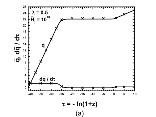
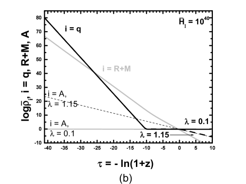
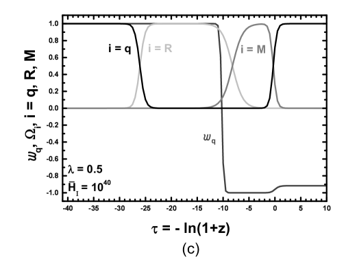
Figure 1: The evolution as a function of $\tau$$\iota$ for ${\mbox{$\leavevmode\hbox{\footnotesize$\tau$\kern-4.0pt$\iota$}_{{}_{\rm I}}$}}=-41$ and ${\mbox{$\bar{H}_{{}_{\rm I}}$}}=10^{40}$ of the quantities: $q$ and $q^{\prime}$ for $\lambda=0.5~{}({\mbox{$\bar{V}_{o}$}}=1.6\times 10^{8})$ (crosses are obtained by our analytical expressions) (a), $\log{\mbox{$\bar{\rho}$}}_{i}$ with $i=q$ (bold black lines), A (thin black lines) and R+M (light grey line) for $\lambda=0.1~{}({\mbox{$\bar{V}_{o}$}}=33.5)$ (solid lines) or $\lambda=1.15~{}({\mbox{$\bar{V}_{o}$}}=1.35\times 10^{19})$ (dashed lines) (b), $w_{q}$ (dark gray line) and $\Omega_{i}$ with $i=q$ (black line), R (light gray line) and M (gray line) for $\lambda=0.5~{}({\mbox{$\bar{V}_{o}$}}=1.6\times 10^{8})$ (c).

We illustrate the evolution of the various quintessential quantities presenting diagrams where in the $x$-axis, $\leavevmode\hbox{\normalsize$\tau$\kern-5.0pt$\iota$}=-\ln(1+z)$ varies from $\leavevmode\hbox{\normalsize$\tau$\kern-5.0pt$\iota$}_{{}_{\rm I}}$ down to late times, e.g. 10 [23, 25, 31].

In fig. 1-(a), we display $q$ and $q^{\prime}$ versus $\tau$$\iota$ for ${\mbox{$\leavevmode\hbox{\normalsize$\tau$\kern-5.0pt$\iota$}_{{}_{\rm I}}$}}=-41$, ${\mbox{$\bar{H}_{{}_{\rm I}}$}}=10^{40}$ and $\lambda=0.5~{}({\mbox{$\bar{V}_{o}$}}=1.6\times 10^{8})$. Solid lines [crosses] are obtained by numerically solving eq. (10) [applying the analytical expressions of sec. 2.2]. Despite their simplicity, our semi-analytical expressions in eqs. (20), (24) and (28), reproduce impressively the numerical evolution of $q$ and $q^{\prime}$.

In fig. 1-(b), we draw $\log{\mbox{$\bar{\rho}$}}_{i}$ versus $\tau$$\iota$ for ${\mbox{$\leavevmode\hbox{\normalsize$\tau$\kern-5.0pt$\iota$}_{{}_{\rm I}}$}}=-41$, ${\mbox{$\bar{H}_{{}_{\rm I}}$}}=10^{40}$ and two “extreme” (see figs. 3-(a) and (b)) values of $\lambda$, $\lambda=0.1~{}({\mbox{$\bar{V}_{o}$}}=33.5)$ (solid lines) or $\lambda=1.15~{}({\mbox{$\bar{V}_{o}$}}=1.35\times 10^{19})$ (dashed lines). For $i=q$ (bold black lines), we show $\log{\mbox{$\bar{\rho}$}}_{q}$, computed by inserting in eq. (11b) the numerical solution of eqs. (10a) and (10b). For $i={\rm A}$ (thin black lines), we show $\log{\mbox{$\bar{\rho}$}}_{{}_{\rm A}}$ derived from eq. (30). For $i={\rm R+M}$ (light grey line), we show $\log{\mbox{$\bar{\rho}$}}_{{}_{\rm R+M}}$, which is the logarithm of the sum of the contributions given by eqs. (8a) and (8b).

In fig. 1-(c), we plot $w_{q}$ (dark gray line) and $\Omega_{i}$ with $i=q$ (black line), R (light gray line) and M (gray line) versus $\tau$$\iota$, for ${\mbox{$\leavevmode\hbox{\normalsize$\tau$\kern-5.0pt$\iota$}_{{}_{\rm I}}$}}=-41$, ${\mbox{$\bar{H}_{{}_{\rm I}}$}}=10^{40}$ and $\lambda=0.5~{}({\mbox{$\bar{V}_{o}$}}=1.6\times 10^{8})$. The $y$-axis quantities are computed by inserting in eqs. (14) and (13) the numerical values obtained by eqs. (11a), (11b) and (8).

Analyzing comparatively figs. 2-(a), (b) and (c), we can demonstrate the characteristic features of the cosmological history in the presence of $q$. In particular:

• For ${\mbox{$\leavevmode\hbox{\normalsize$\tau$\kern-5.0pt$\iota$}_{{}_{\rm I}}$}}\leq\leavevmode\hbox{\normalsize$\tau$\kern-5.0pt$\iota$}\leq{\mbox{$\leavevmode\hbox{\normalsize$\tau$\kern-5.0pt$\iota$}_{{}_{\rm KR}}$}}=-26.2$, the universe undergoes the KD era. The field $q$ increases according to eq. (20) along the left inclined part of the curve in fig. 1-(a) and ${\mbox{$\bar{\rho}$}}_{q}$ decreases, more steeply than ${\mbox{$\bar{\rho}$}}_{{}_{\rm R}}$, according to eq. (19), along the left inclined part of the black solid curve in fig. 1-(b). During this period, $w_{q}=1$, as shown in fig. 1-(c). This era terminates at $\leavevmode\hbox{\normalsize$\tau$\kern-5.0pt$\iota$}_{{}_{\rm KR}}$, where an intersection of ${\mbox{$\bar{\rho}$}}_{q}~{}[\Omega_{q}]$ with ${\mbox{$\bar{\rho}$}}_{{}_{\rm R}}~{}[\Omega_{\rm R}]$ is observed in fig. 1-(b) [fig. 1-(c)].

• For ${\mbox{$\leavevmode\hbox{\normalsize$\tau$\kern-5.0pt$\iota$}_{{}_{\rm KR}}$}}=-26.2\leq\leavevmode\hbox{\normalsize$\tau$\kern-5.0pt$\iota$}\leq\leavevmode\hbox{\normalsize$\tau$\kern-5.0pt$\iota$}_{{}_{\rm FA}}=0.67$, the universe undergoes successively the RD era and then the MD era until the re-appearance of DE. More precisely, $q$ freezes to its constant value ${\mbox{$\bar{q}$}}_{{}_{\rm F}}\simeq 22.4$ according to eq. (24) (or eq. (25) for $\leavevmode\hbox{\normalsize$\tau$\kern-5.0pt$\iota$}\geq\leavevmode\hbox{\normalsize$\tau$\kern-5.0pt$\iota$}_{{}_{\rm KF}}=-20.2$) along the horizontal part of the curve in fig. 1-(a). $\Omega_{\rm R}>\Omega_{q}$ increases towards 1 along the light gray line of fig. 1-(c) and then decreases until $\Omega_{{}_{\rm M}}=\Omega_{{}_{\rm R}}$ at $\leavevmode\hbox{\normalsize$\tau$\kern-5.0pt$\iota$}_{\rm eq}=-8.16$, where a slight kink is observed on the light gray line of fig. 1-(b). For $\leavevmode\hbox{\normalsize$\tau$\kern-5.0pt$\iota$}_{{}_{\rm KF}}\leq\leavevmode\hbox{\normalsize$\tau$\kern-5.0pt$\iota$}\leq\leavevmode\hbox{\normalsize$\tau$\kern-5.0pt$\iota$}_{{}_{\rm PL}}=-10.22$, ${\mbox{$\bar{\rho}$}}_{q}<{\mbox{$\bar{\rho}$}}_{{}_{\rm R}}$ continues to decrease steeply according to eq. (19), along the left inclined part of the black solid curve in fig. 1-(b), while $w_{q}$ continues to be 1 as shown in fig. 1-(c). On the other hand, for $\leavevmode\hbox{\normalsize$\tau$\kern-5.0pt$\iota$}_{{}_{\rm PL}}\leq\leavevmode\hbox{\normalsize$\tau$\kern-5.0pt$\iota$}\leq\leavevmode\hbox{\normalsize$\tau$\kern-5.0pt$\iota$}_{{}_{\rm FA}}$, ${\mbox{$\bar{\rho}$}}_{q}$ freezes to its constant value ${\mbox{$\bar{\rho}$}}_{q_{\rm F}}={\mbox{$\bar{V}$}}({\mbox{$\bar{q}$}}_{{}_{\rm F}})=0.62$ in fig. 1-(b), while $w_{q}$ transits from 1 to -1 as shown in fig. 1-(c). At present, we obtain $w_{q}(0)=-0.96$, within the limits of eq. (34).

• For $\leavevmode\hbox{\normalsize$\tau$\kern-5.0pt$\iota$}\geq\leavevmode\hbox{\normalsize$\tau$\kern-5.0pt$\iota$}_{{}_{\rm FA}}=0.67$, the universe undergoes a $q$-dominated phase. The field $q$ increases according to eq. (28) along the right inclined part of the curve in fig. 1-(a), ${\mbox{$\bar{\rho}$}}_{q}$ decreases according to eq. (30) along the right inclined parts of the curves in fig. 1-(b) for $\lambda=0.1$ and 1.15, while $w_{q}$ in fig. 1-(c) tends to its fixed-point value for $\lambda=0.5$, $w_{q}^{\rm fp}=-0.92$. As shown in the same figure $\Omega^{\rm fp}_{q}=1$, which identifies the late-time attractor.

Note that, contrary to the case with $\lambda>2$ [41], the variation of $\lambda$ does not affect essentially the position of the FD plateau but only changes the inclination of the AD curve.

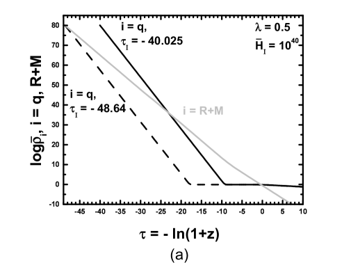
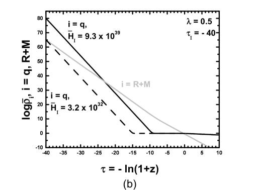
Figure 2: The evolution of the quantities $\log{\mbox{$\bar{\rho}$}}_{i}$ with $i=q$ (black lines) and R+M (light grey line) as a function of $\tau$$\iota$ for $\lambda=0.5$ and: ${\mbox{$\bar{H}$}}_{\rm I}=10^{40}$ and ${\mbox{$\leavevmode\hbox{\footnotesize$\tau$\kern-4.0pt$\iota$}_{{}_{\rm I}}$}}=-40.025~{}({\mbox{$\bar{V}_{o}$}}=1.6\times 10^{9})$ [${\mbox{$\leavevmode\hbox{\footnotesize$\tau$\kern-4.0pt$\iota$}_{{}_{\rm I}}$}}=-48.64~{}({\mbox{$\bar{V}_{o}$}}=2.3)$] (solid [dashed] line) (a), ${\mbox{$\leavevmode\hbox{\footnotesize$\tau$\kern-4.0pt$\iota$}_{{}_{\rm I}}$}}=-40$ and ${\mbox{$\bar{H}_{{}_{\rm I}}$}}=9.3\times 10^{39}~{}({\mbox{$\bar{V}_{o}$}}=1.6\times 10^{9})$ [${\mbox{$\bar{H}$}}_{\rm I}=3.2\times 10^{32}~{}({\mbox{$\bar{V}_{o}$}}=2.3)$] (solid [dashed] line) (b).

The dependence of the ${\mbox{$\bar{\rho}$}}_{q}$ evolution on ${\mbox{$\leavevmode\hbox{\normalsize$\tau$\kern-5.0pt$\iota$}_{{}_{\rm I}}$}}~{}[{\mbox{$\bar{H}_{{}_{\rm I}}$}}]$, can be easily concluded from fig. 2-(a) [fig. 2-(b)], where we plot for $\lambda=0.5$, $\log{\mbox{$\bar{\rho}$}}_{q}$ and $\log{\mbox{$\bar{\rho}$}}_{{}_{\rm R+M}}$ versus $\tau$$\iota$. In fig. 2-(a) [fig. 2-(b)] we take ${\mbox{$\bar{H}$}}_{\rm I}=10^{40}$ and ${\mbox{$\leavevmode\hbox{\normalsize$\tau$\kern-5.0pt$\iota$}_{{}_{\rm I}}$}}=-40.025~{}({\mbox{$\bar{V}_{o}$}}=1.6\times 10^{9})$ (solid line) or ${\mbox{$\leavevmode\hbox{\normalsize$\tau$\kern-5.0pt$\iota$}_{{}_{\rm I}}$}}=-48.64~{}({\mbox{$\bar{V}_{o}$}}=2.3)$ (dashed line) [${\mbox{$\leavevmode\hbox{\normalsize$\tau$\kern-5.0pt$\iota$}_{{}_{\rm I}}$}}=-40$ and ${\mbox{$\bar{H}_{{}_{\rm I}}$}}=9.3\times 10^{39}~{}({\mbox{$\bar{V}_{o}$}}=1.6\times 10^{9})$ (solid line) or ${\mbox{$\bar{H}$}}_{\rm I}=3.2\times 10^{32}~{}({\mbox{$\bar{V}_{o}$}}=2.3)$ (dashed line)]. It is obvious that increasing $\leavevmode\hbox{\normalsize$\tau$\kern-5.0pt$\iota$}_{{}_{\rm I}}$ or $\bar{H}_{{}_{\rm I}}$, the left, black inclined line of the $q$-KD regime moves to the right and consequently, both $\Omega_{q}({\mbox{$\leavevmode\hbox{\normalsize$\tau$\kern-5.0pt$\iota$}_{{}_{\rm I}}$}})$ and $\Omega_{q}({\mbox{$\leavevmode\hbox{\normalsize$\tau$\kern-5.0pt$\iota$}_{{}_{\rm NS}}$}})$ increase. So, an upper [lower] bound on $\leavevmode\hbox{\normalsize$\tau$\kern-5.0pt$\iota$}_{{}_{\rm I}}$ or $\bar{H}_{{}_{\rm I}}$ can be extracted from eq. (32) [eq. (31)] (see fig. 3). The saturation of these inequalities is the origin of the chosen lower [upper] $\leavevmode\hbox{\normalsize$\tau$\kern-5.0pt$\iota$}_{{}_{\rm I}}$ or $\bar{H}_{{}_{\rm I}}$ in fig. 2.

4.2 IMPOSING THE QUINTESSENTIAL REQUIREMENTS

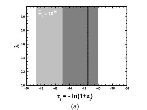
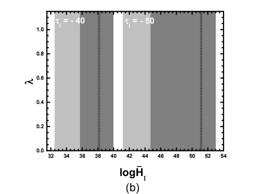
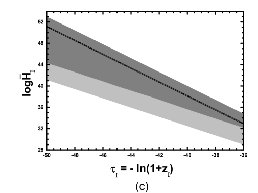
Figure 3: The allowed (shaded) areas on the ${\mbox{$\leavevmode\hbox{\footnotesize$\tau$\kern-4.0pt$\iota$}_{{}_{\rm I}}$}}-\lambda$ plane for ${\mbox{$\bar{H}_{{}_{\rm I}}$}}=10^{40}$ (a), $\log{\mbox{$\bar{H}_{{}_{\rm I}}$}}-\lambda$ plane for ${\mbox{$\leavevmode\hbox{\footnotesize$\tau$\kern-4.0pt$\iota$}_{{}_{\rm I}}$}}=-40$ or ${\mbox{$\leavevmode\hbox{\footnotesize$\tau$\kern-4.0pt$\iota$}_{{}_{\rm I}}$}}=-50$ (b) and ${\mbox{$\leavevmode\hbox{\footnotesize$\tau$\kern-4.0pt$\iota$}_{{}_{\rm I}}$}}-\log{\mbox{$\bar{H}_{{}_{\rm I}}$}}$ plane for $\lambda=0.5$ (c). Lined are, also, the areas allowed by eq. (2) for $m_{\chi}=350~{}{\rm GeV}$ and $\langle\sigma v\rangle=10^{-7}~{}{\rm GeV}^{-2}$.

We proceed, now in the delineation of the parameter space of our quintessential model. Agreement with eq. (34) entails $0<\lambda\lesssim 1.15$ (see also ref. [25], where less restrictive upper bound on $w_{q}(0)$ was imposed). This range is independent on $\leavevmode\hbox{\normalsize$\tau$\kern-5.0pt$\iota$}_{{}_{\rm I}}$ and $\bar{H}_{{}_{\rm I}}$ as is shown in figs. 3-(a) and 3-(b). In these, we depict respectively the allowed (shaded) regions on the ${\mbox{$\leavevmode\hbox{\normalsize$\tau$\kern-5.0pt$\iota$}_{{}_{\rm I}}$}}-\lambda$ plane for ${\mbox{$\bar{H}_{{}_{\rm I}}$}}=10^{40}$ and on the $\log{\mbox{$\bar{H}_{{}_{\rm I}}$}}-\lambda$ plane for ${\mbox{$\leavevmode\hbox{\normalsize$\tau$\kern-5.0pt$\iota$}_{{}_{\rm I}}$}}=-40$ or ${\mbox{$\leavevmode\hbox{\normalsize$\tau$\kern-5.0pt$\iota$}_{{}_{\rm I}}$}}=-50$. In fig. 3-(c), we design the allowed area on the ${\mbox{$\leavevmode\hbox{\normalsize$\tau$\kern-5.0pt$\iota$}_{{}_{\rm I}}$}}-\log{\mbox{$\bar{H}_{{}_{\rm I}}$}}$ plane. Although this plot is constructed for $\lambda=0.5$, it is obviously $\lambda$ independent. The dark [light] shaded areas fulfill eq. (31a) [eq. (31b) and (31c)]. The right [left] boundaries of the allowed regions in figs. 3-(a) and 3-(b) are derived from eq. (32) [eq. (31b)]. The same origin has the upper [lower] boundary of the allowed region in fig. 3-(c), whereas the left and right boundaries come from eq. (35a). So, for a reasonable set of ($\lambda,{\mbox{$\leavevmode\hbox{\normalsize$\tau$\kern-5.0pt$\iota$}_{{}_{\rm I}}$}},{\mbox{$\bar{H}_{{}_{\rm I}}$}}$), the exponential quintessential model can become consistent with the observational data [23, 25]. The construction of the ruled areas is explained in sec. 4.4.2.

4.3 THE $\Omega_{\chi}h_{0}^{2}$ ENHANCEMENT

The investigation of the $\Omega_{\chi}h_{0}^{2}$ enhancement is the aim of this section. In sec. 4.3.1, we illustrate the $\chi$ decoupling during the KD epoch and in sec. 4.3.2 we examine the dependence of the $\Omega_{\chi}h_{0}^{2}$ increase on $\Omega_{q}({\mbox{$\leavevmode\hbox{\normalsize$\tau$\kern-5.0pt$\iota$}_{{}_{\rm NS}}$}})$. Finally, in sec. 4.3.3, we compare the results of our numerical and semi-analytical $\Omega_{\chi}h_{0}^{2}$ calculations.

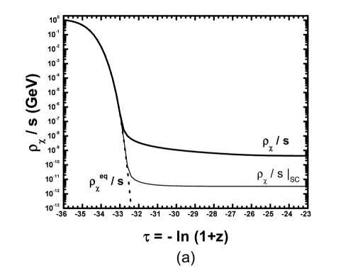
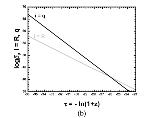
Input Parameters
$\lambda$	$\leavevmode\hbox{\normalsize$\tau$\kern-5.0pt$\iota$}_{{}_{\rm I}}$	$\bar{H}_{{}_{\rm I}}$	$\bar{V}_{o}$	$m_{\chi}({\rm GeV})$	${\mbox{$\langle\sigma v\rangle$}}({\rm GeV}^{-2})$
$0.5$	$-41$	$10^{40}$	$1.6\times 10^{8}$	$350$	$2.92\times 10^{-7}$
Output Parameters
$\Omega_{q}(\leavevmode\hbox{\normalsize$\tau$\kern-5.0pt$\iota$}_{{}_{\rm NS}})$	$\leavevmode\hbox{\normalsize$\tau$\kern-5.0pt$\iota$}_{{}_{\rm F}}$	${\mbox{$\leavevmode\hbox{\normalsize$\tau$\kern-5.0pt$\iota$}_{{}_{\rm F}}$}}|_{{}_{\rm SC}}$	$\leavevmode\hbox{\normalsize$\tau$\kern-5.0pt$\iota$}_{{}_{\rm KR}}$	$\Omega_{\chi}h_{0}^{2}$	$\Delta\Omega_{\chi}$
$0.0007$	$-32.9$	$-32.6$	$-25.7$	$0.115$	$126.8$

Figure 4: The evolution as a function of $\tau$$\iota$ of the quantities $\rho^{\rm eq}_{\chi}/s$ (dotted line) and $\rho_{\chi}/s$ (bold [thin] solid lines) for the quintessential scenario [SC] ${\sf(a)}$ and $\log{\mbox{$\bar{\rho}$}}_{i}$ with $i=q~{}[i=R]$ (black [light grey] line) ${\sf(b)}$ for the input quantities listed in the table above.

4.3.1 The $\chi$ decoupling.

The $\chi$ decoupling during the KD era is instructively displayed in figs. 4-(a) and (b). In fig. 4-(a) we depict $\rho^{[\rm eq]}_{\chi}/s$ (dotted lines) and $\rho_{\chi}/s~{}[\rho_{\chi}/s|_{{}_{\rm SC}}~{}(\mbox{for}~{}g_{q}=1)]$ (bold [thin] solid lines) versus $\tau$$\iota$. In fig. 4-${\sf(b)}$, we plot $\log{\mbox{$\bar{\rho}$}}_{q}~{}[\log{\mbox{$\bar{\rho}$}}_{{}_{\rm R}}]$ (black [light gray] line) versus $\tau$$\iota$. The needed for our calculation inputs and some key-outputs are listed in the relevant table. For better comparison, we give, also, the point of the $\chi$ decoupling, in the case of the SC ($g_{q}=1$), ${\mbox{$\leavevmode\hbox{\normalsize$\tau$\kern-5.0pt$\iota$}_{{}_{\rm F}}$}}|_{{}_{\rm SC}}$. In the present case, the $\chi$ decoupling is realized deeply within the KD regime, ${\mbox{$\leavevmode\hbox{\normalsize$\tau$\kern-5.0pt$\iota$}_{{}_{\rm I}}$}}<{\mbox{$\leavevmode\hbox{\normalsize$\tau$\kern-5.0pt$\iota$}_{{}_{\rm F}}$}}<{\mbox{$\leavevmode\hbox{\normalsize$\tau$\kern-5.0pt$\iota$}_{{}_{\rm KR}}$}}$ and ${\mbox{$\leavevmode\hbox{\normalsize$\tau$\kern-5.0pt$\iota$}_{{}_{\rm F}}$}}<{\mbox{$\leavevmode\hbox{\normalsize$\tau$\kern-5.0pt$\iota$}_{{}_{\rm F}}$}}|_{{}_{\rm SC}}$. By adjusting $\langle\sigma v\rangle$ we extract the central $\Omega_{\chi}h_{0}^{2}$ in eq. (2). The presence of the KD era causes an efficient $\Omega_{\chi}h_{0}^{2}$ enhancement, $\Delta\Omega_{\chi}=126.8$ ($\Omega_{\chi}h_{0}^{2}|_{{}_{\rm SC}}=0.0009$). Note that the condition ${\mbox{$\leavevmode\hbox{\normalsize$\tau$\kern-5.0pt$\iota$}_{{}_{\rm F}}$}}<{\mbox{$\leavevmode\hbox{\normalsize$\tau$\kern-5.0pt$\iota$}_{{}_{\rm KR}}$}}$ is indispensable in order to obtain sizable $\Delta\Omega_{\chi}$. This can be understood as follows. From eqs. (21) and (10) we obtain ${\mbox{$\leavevmode\hbox{\normalsize$\tau$\kern-5.0pt$\iota$}_{{}_{\rm KR}}$}}\simeq{\mbox{$\leavevmode\hbox{\normalsize$\tau$\kern-5.0pt$\iota$}_{{}_{\rm NS}}$}}+\ln r_{{}_{\rm NS}}/2$. If we demand ${\mbox{$\leavevmode\hbox{\normalsize$\tau$\kern-5.0pt$\iota$}_{{}_{\rm KR}}$}}<{\mbox{$\leavevmode\hbox{\normalsize$\tau$\kern-5.0pt$\iota$}_{{}_{\rm F}}$}}$, we obtain $\Omega_{q}({\mbox{$\leavevmode\hbox{\normalsize$\tau$\kern-5.0pt$\iota$}_{{}_{\rm NS}}$}})<7.7\times 10^{-10}$, which causes a very weak $\Delta\Omega_{\chi}<2.2$. Finally, the phenomenon of re-annihilation [37] is not observed in this context. This is, because in our case $H$ smoothly evolves from its KD to RD behaviour – see eq. (8) – and does not sharply drop after the $\chi$-decoupling as in the case of ref. [37].

4.3.2 The dependence of $\Delta\Omega_{\chi}$ on $\Omega_{q}({\mbox{$\leavevmode\hbox{\normalsize$\tau$\kern-5.0pt$\iota$}_{{}_{\rm NS}}$}})$.

As is shown in figs. 2-(a) and 2-(b), the position of the inclined left part of the black line (corresponding to $\log{\mbox{$\bar{\rho}$}}_{q}$) is affected crucially by a possible variation of $\leavevmode\hbox{\normalsize$\tau$\kern-5.0pt$\iota$}_{{}_{\rm I}}$ or $\bar{H}_{{}_{\rm I}}$ but not of $\lambda$. Therefore, $\Omega_{q}({\mbox{$\leavevmode\hbox{\normalsize$\tau$\kern-5.0pt$\iota$}_{{}_{\rm NS}}$}})$ and consequently, $\Delta\Omega_{\chi}$ (see eqs. (8) and (10)) depend on $\leavevmode\hbox{\normalsize$\tau$\kern-5.0pt$\iota$}_{{}_{\rm I}}$ or $\bar{H}_{{}_{\rm I}}$ but not on $\lambda$ (contrary to the case of ref. [41]). Moreover, the dependence of $\Delta\Omega_{\chi}$ on $\leavevmode\hbox{\normalsize$\tau$\kern-5.0pt$\iota$}_{{}_{\rm I}}$ or $\bar{H}_{{}_{\rm I}}$ can be expressed exclusively as a single-valued function of $\Omega_{q}({\mbox{$\leavevmode\hbox{\normalsize$\tau$\kern-5.0pt$\iota$}_{{}_{\rm NS}}$}})$, since only $g_{q}$ is involved in the $\Omega_{\chi}h_{0}^{2}$ calculation (see eqs. (19) and (17)). This is illustrated in the fig. 5, where we depict iso-$\Omega_{q}({\mbox{$\leavevmode\hbox{\normalsize$\tau$\kern-5.0pt$\iota$}_{{}_{\rm NS}}$}})$ lines on the allowed region of the ${\mbox{$\leavevmode\hbox{\normalsize$\tau$\kern-5.0pt$\iota$}_{{}_{\rm I}}$}}-\log{\mbox{$\bar{H}_{{}_{\rm I}}$}}$ plane, presented in fig. 3-(c). Along these lines, $\Delta\Omega_{\chi}$ remains, also, constant (indicated in the table of fig. 5) for fixed $m_{\chi}=350~{}{\rm GeV}$ and $\langle\sigma v\rangle=10^{-10}~{}{\rm GeV^{-2}}$ or $\langle\sigma v\rangle=10^{-7}~{}{\rm GeV^{-2}}$. Consequently, the number of the free $q$ parameters $({\mbox{$\leavevmode\hbox{\normalsize$\tau$\kern-5.0pt$\iota$}_{{}_{\rm I}}$}},~{}{\mbox{$\bar{H}_{{}_{\rm I}}$}})$, which determine $\Delta\Omega_{\chi}$, can be reduced by one and replaced by $\Omega_{q}({\mbox{$\leavevmode\hbox{\normalsize$\tau$\kern-5.0pt$\iota$}_{{}_{\rm NS}}$}})$.

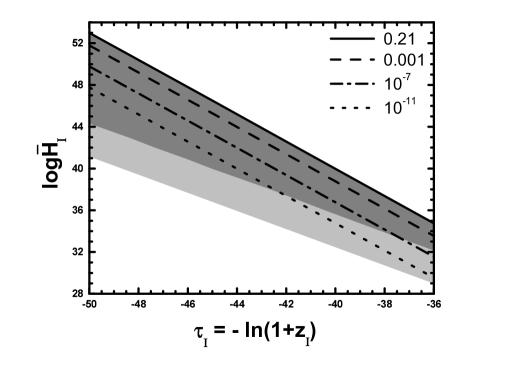
Figure 5: Lines with constant $\Omega_{q}(\leavevmode\hbox{\footnotesize$\tau$\kern-4.0pt$\iota$}_{{}_{\rm NS}})$, indicated in the plot, in the allowed ${\mbox{$\leavevmode\hbox{\footnotesize$\tau$\kern-4.0pt$\iota$}_{{}_{\rm I}}$}}-\log{\mbox{$\bar{H}_{{}_{\rm I}}$}}$ plane. The corresponding constant values of $\Delta\Omega_{\chi}$ for $m_{\chi}=350~{}{\rm GeV}$ and $\langle\sigma v\rangle=10^{-10}~{}{\rm GeV^{-2}}$ or $\langle\sigma v\rangle=10^{-7}~{}{\rm GeV^{-2}}$ are also listed in the table.

4.3.3 Numerical Versus Semi-Analytical Results.

The validity of our semi-analytical approach can be tested by comparing its results for $\Delta\Omega_{\chi}$ with those obtained by the numerical solution of eqs. (4). In addition, useful conclusions can be inferred for the behavior of $\Delta\Omega_{\chi}$ as a function of our free parameters, $m_{\chi},~{}{\mbox{$\langle\sigma v\rangle$}}$ and $\Omega_{q}(\leavevmode\hbox{\footnotesize$\tau$\kern-4.0pt$\iota$}_{{}_{\rm NS}})$. Our results are presented in fig. 6. The solid and dashed lines are drawn from our numerical code, whereas crosses are obtained by employing the formulas of sec. 3.3 with $\delta_{\rm F}=1.28~{}[\delta_{\rm F}=1.35]$ for ${\mbox{$\langle\sigma v\rangle$}}=a~{}[\langle\sigma v\rangle=bx]$. In figs. 6-$\sf(a_{1})$ [6-$\sf(a_{2})$], we present $\Delta\Omega_{\chi}$ versus $\Omega_{q}(\leavevmode\hbox{\normalsize$\tau$\kern-5.0pt$\iota$}_{{}_{\rm NS}})$ for $\langle\sigma v\rangle=10^{-10}~{}{\rm GeV^{-2}}~{}[\langle\sigma v\rangle=10^{-10}x~{}{\rm GeV^{-2}}]$. We take $m_{\chi}=200~{}{\rm GeV}~{}[m_{\chi}=500~{}{\rm GeV}]$ (light [normal] grey lines and crosses). In fig. 6-(b), we plot $\Delta\Omega_{\chi}$ versus $a=\langle\sigma v\rangle~{}[a=\langle\sigma v\rangle/x]$ for $m_{\chi}=350~{}{\rm GeV}$ and $\langle\sigma v\rangle=a~{}[\langle\sigma v\rangle=ax]$ (solid [dashed] lines). In fig. 6-(c), we depict $\Delta\Omega_{\chi}$ versus $m_{\chi}$ for $\langle\sigma v\rangle=10^{-10}~{}{\rm GeV}^{-2}~{}[\langle\sigma v\rangle=10^{-10}x~{}{\rm GeV}^{-2}]$ (solid [dashed] lines). In the last two cases, we use $\Omega_{q}(\leavevmode\hbox{\normalsize$\tau$\kern-5.0pt$\iota$}_{{}_{\rm NS}})=0.001~{}[\Omega_{q}(\leavevmode\hbox{\normalsize$\tau$\kern-5.0pt$\iota$}_{{}_{\rm NS}})=0.1]$ (light [normal] grey lines and crosses). As we anticipated in sec. 3.3.4, $\Delta\Omega_{\chi}$ increases when $\Omega_{q}({\mbox{$\leavevmode\hbox{\normalsize$\tau$\kern-5.0pt$\iota$}_{{}_{\rm NS}}$}})$ (see figs. 6-${\sf(a_{1})}$ and ${\sf(a_{2})}$) or $m_{\chi}$ (see fig.  6-(c)) increases and when $\langle\sigma v\rangle$ decreases (see fig. 6-(b)). From figs. 6-(b) and 6-(c) is, also, deduced that $\Delta\Omega_{\chi}$ increases more drastically in the ${\mbox{$\langle\sigma v\rangle$}}=bx$ case than in the ${\mbox{$\langle\sigma v\rangle$}}=a$ case for $a=b$ and fixed $m_{\chi}$ and $\Omega_{q}(\leavevmode\hbox{\normalsize$\tau$\kern-5.0pt$\iota$}_{{}_{\rm NS}})$. Evident is, finally, the agreement between numerical and semi-analytical results.

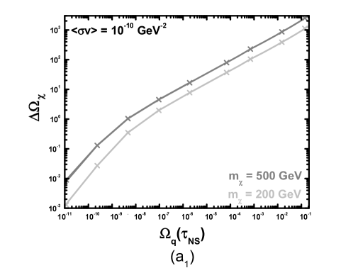
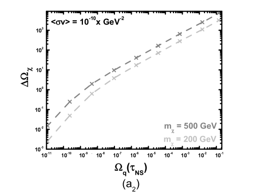
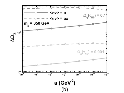
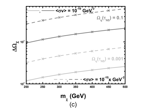
Figure 6: $\Delta\Omega_{\chi}$ versus $\Omega_{q}(\leavevmode\hbox{\footnotesize$\tau$\kern-4.0pt$\iota$}_{{}_{\rm NS}})$ for $m_{\chi}=200~{}{\rm GeV}~{}[m_{\chi}=500~{}{\rm GeV}]$ (light [normal] grey lines and crosses) and $\langle\sigma v\rangle=10^{-10}~{}{\rm GeV^{-2}}~{}[\langle\sigma v\rangle=10^{-10}x~{}{\rm GeV^{-2}}]~{}{\sf(a_{1}~{}[a_{2}])}$. Also, $\Delta\Omega_{\chi}$ versus $a=\langle\sigma v\rangle~{}[a=\langle\sigma v\rangle/x]$ for $m_{\chi}=350~{}{\rm GeV}$ and $\langle\sigma v\rangle=a~{}[\langle\sigma v\rangle=ax]$ (solid [dashed] lines) (b) and $\Delta\Omega_{\chi}$ versus $m_{\chi}$ for $\langle\sigma v\rangle=10^{-10}~{}{\rm GeV}^{-2}~{}[\langle\sigma v\rangle=10^{-10}x~{}{\rm GeV}^{-2}]$ (solid [dashed] lines) (c). We take $\Omega_{q}(\leavevmode\hbox{\footnotesize$\tau$\kern-4.0pt$\iota$}_{{}_{\rm NS}})=0.001~{}[\Omega_{q}(\leavevmode\hbox{\footnotesize$\tau$\kern-4.0pt$\iota$}_{{}_{\rm NS}})=0.1]$ (light [normal] grey lines and crosses). The solid or dashed lines [crosses] are obtained by our numerical code [semi-analytical expressions].

4.4 IMPOSING THE CDM REQUIREMENT

Requiring $\Omega_{\chi}h_{0}^{2}$ to be confined in the cosmologically allowed range of eq. (2), one can restrict not only the CDM parameters (see subsec. 4.4.1) but also the $q$ parameters, $\lambda,~{}{\mbox{$\leavevmode\hbox{\normalsize$\tau$\kern-5.0pt$\iota$}_{{}_{\rm I}}$}}$ and $\bar{H}_{{}_{\rm I}}$ (see subsec. 4.4.2) or $\Omega_{q}({\mbox{$\leavevmode\hbox{\normalsize$\tau$\kern-5.0pt$\iota$}_{{}_{\rm NS}}$}})$ (see subsec. 4.4.3). The data is derived exclusively by the numerical program. Let us note, in passing, that bounds arisen from eq. (2b), are more rigorous than those originated from eq. (2a), since other production mechanisms of $\chi$’s may be activated [36, 65] and/or other CDM candidates [4] may contribute to $\Omega_{\rm CDM}$.

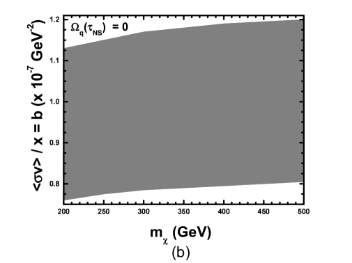
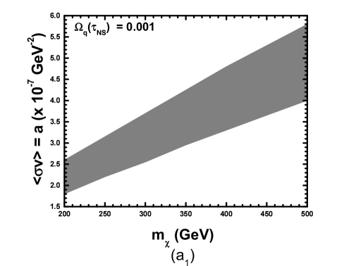
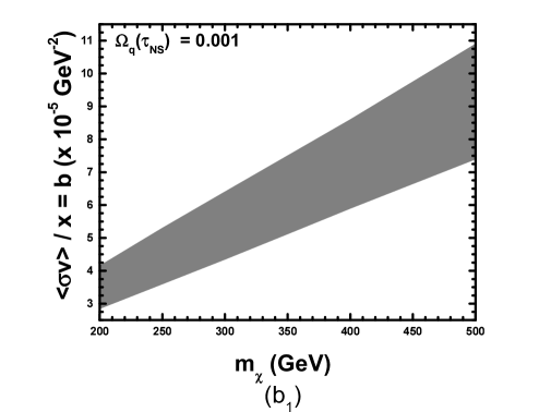
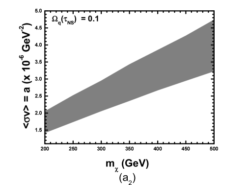
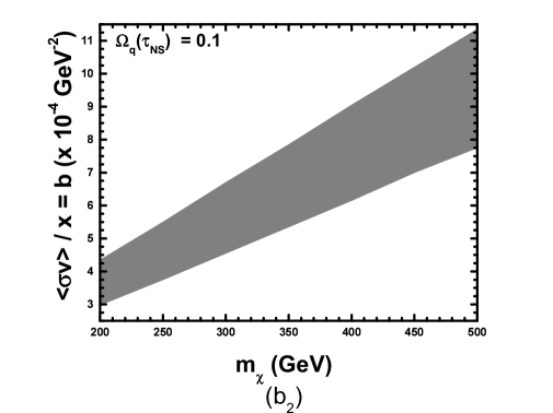
Figure 7: The allowed region on the $m_{\chi}-{\mbox{$\langle\sigma v\rangle$}}$ plane for ${\mbox{$\langle\sigma v\rangle$}}=a$ ${\sf(a,~{}a_{1},~{}a_{2})}$ or on the $m_{\chi}-{\mbox{$\langle\sigma v\rangle$}}/x$ plane for ${\mbox{$\langle\sigma v\rangle$}}=bx$ ${\sf(b,~{}b_{1},~{}b_{2})}$. We take $\Omega_{q}({\mbox{$\leavevmode\hbox{\normalsize$\tau$\kern-5.0pt$\iota$}_{{}_{\rm NS}}$}})=0.001~{}[\Omega_{q}({\mbox{$\leavevmode\hbox{\normalsize$\tau$\kern-5.0pt$\iota$}_{{}_{\rm NS}}$}})=0.1]$ in fig. ${\sf(a_{1},~{}b_{1})}$ [fig. ${\sf(a_{2},~{}b_{2})}$] whereas, for the sake of comparison, we consider the SC ($\Omega_{q}({\mbox{$\leavevmode\hbox{\normalsize$\tau$\kern-5.0pt$\iota$}_{{}_{\rm NS}}$}})=0$) in figs. (a) and (b).

4.4.1 Constraining the CDM parameters.

Fixing the $q$ parameters, we can derive restrictions on the CDM parameters. Namely, in fig. 7 we construct the allowed regions on the $m_{\chi}-{\mbox{$\langle\sigma v\rangle$}}$ plane for ${\mbox{$\langle\sigma v\rangle$}}=a$ ${\sf(a,~{}a_{1},~{}a_{2})}$ or on the $m_{\chi}-{\mbox{$\langle\sigma v\rangle$}}/x$ plane for ${\mbox{$\langle\sigma v\rangle$}}=bx$ ${\sf(b,~{}b_{1},~{}b_{2})}$. As we showed in subsec. 4.3.2, the $q$ parameters can be replaced by $\Omega_{q}({\mbox{$\leavevmode\hbox{\normalsize$\tau$\kern-5.0pt$\iota$}_{{}_{\rm NS}}$}})$. So, in figs. 7-${\sf(a_{1})}$ and ${\sf(b_{1})}$ [figs. 7-${\sf(a_{2})}$ and ${\sf(b_{2})}$], we fix $\Omega_{q}({\mbox{$\leavevmode\hbox{\normalsize$\tau$\kern-5.0pt$\iota$}_{{}_{\rm NS}}$}})=0.001~{}[\Omega_{q}({\mbox{$\leavevmode\hbox{\normalsize$\tau$\kern-5.0pt$\iota$}_{{}_{\rm NS}}$}})=0.1]$, whereas in figs. 7-(a) and (b), we consider, for better reference, the SC, with $\Omega_{q}({\mbox{$\leavevmode\hbox{\normalsize$\tau$\kern-5.0pt$\iota$}_{{}_{\rm NS}}$}})=0$. The upper [lower] boundaries of the allowed areas are derived from eq. (2${\sf a}$) [eq. (2${\sf b}$)]. This is due to the fact that $\Omega_{\chi}h_{0}^{2}$ is inverse proportional to $\langle\sigma v\rangle$ as is obvious from eqs. (19) and (17) and so, $\Omega_{\chi}h_{0}^{2}$ decreases as $\langle\sigma v\rangle$ increases (contrary to the case of the non-equilibrium $\chi$ production [35, 36]).

We observe that with $\Omega_{q}({\mbox{$\leavevmode\hbox{\normalsize$\tau$\kern-5.0pt$\iota$}_{{}_{\rm NS}}$}})=0.001~{}[\Omega_{q}({\mbox{$\leavevmode\hbox{\normalsize$\tau$\kern-5.0pt$\iota$}_{{}_{\rm NS}}$}})=0.1]$, agreement with eq. (2) entails almost two [three] orders of magnitude higher $\langle\sigma v\rangle$’s than those required in the SC. Also, due to the presence of $\Omega_{q}({\mbox{$\leavevmode\hbox{\normalsize$\tau$\kern-5.0pt$\iota$}_{{}_{\rm NS}}$}})>0$, $\Omega_{\chi}h_{0}^{2}$ increases with $m_{\chi}$ more dramatically than in the case of the SC ($\Omega_{q}({\mbox{$\leavevmode\hbox{\normalsize$\tau$\kern-5.0pt$\iota$}_{{}_{\rm NS}}$}})=0$), illustrated in figs. 7-(a) and (b). This effect is more straightened in the ${\mbox{$\langle\sigma v\rangle$}}=bx$ case, as is seen in figs. 7-${\sf(b_{1})}$ and ${\sf(b_{2})}$.

The requisite high values for $\langle\sigma v\rangle$ (almost unnatural in the ${\mbox{$\langle\sigma v\rangle$}}=bx$ case) can be obtained by resorting to SUSY models which ensure $A$-pole effects [61, 62] or “gaugino-inspired” CANs [57, 58, 59], as in the applications [43, 44] of ref. [41]. Less efficient augmentation of $\langle\sigma v\rangle$ can be achieved by lowering the masses of the CDM candidates in ED models [6, 7, 8] or by employing sfermionic CANs [56, 60, 59] in SUSY models. Consequently, the constrained minimal SUSY model [63], although tightly restricted even in the SC [62, 64], can become consistent with a quintessential KD period, e.g. applying the $A$-pole effects [61, 62].

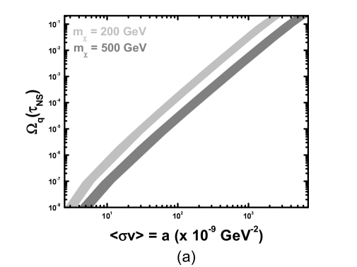
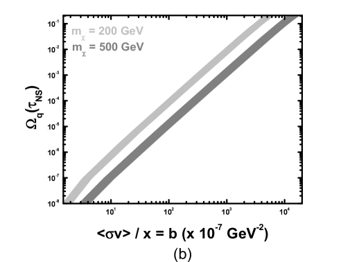
Figure 8: The allowed regions for $m_{\chi}=200~{}{\rm GeV}~{}[m_{\chi}=500~{}{\rm GeV}]$ (light [normal] grey areas) on the ${\mbox{$\langle\sigma v\rangle$}}-\Omega_{q}(\leavevmode\hbox{\footnotesize$\tau$\kern-4.0pt$\iota$}_{{}_{\rm NS}})$ plane for ${\mbox{$\langle\sigma v\rangle$}}=a$ (a) or on the ${\mbox{$\langle\sigma v\rangle$}}/x-\Omega_{q}(\leavevmode\hbox{\footnotesize$\tau$\kern-4.0pt$\iota$}_{{}_{\rm NS}})$ plane for ${\mbox{$\langle\sigma v\rangle$}}=bx$ (b).

4.4.2 Constraining further the $q$ parameters.

Fixing the CDM parameters to naturally obtainable values, $m_{\chi}=350~{}{\rm GeV}$ and ${\mbox{$\langle\sigma v\rangle$}}=10^{-7}~{}{\rm GeV}^{-2}$ (which yield $\Omega_{\chi}h_{0}^{2}|_{{}_{\rm SC}}\simeq 0.0025$), we can constrain further the $q$ parameters, which are already constrained by the quintessential requirements in subsec. 4.2. The regions consistent with the achievement of eq. (2) are ruled in fig. 3. As expected from the argument of subsec. 4.3.2, $\Omega_{q}({\mbox{$\leavevmode\hbox{\normalsize$\tau$\kern-5.0pt$\iota$}_{{}_{\rm NS}}$}})$ turns out to be constant and equal to $8.5\times 10^{-5}~{}[3.6\times 10^{-5}]$ along the right [left] boundaries of the ruled areas in fig. 3-(a), fig. 3-(b) and along the inclined upper [lower] boundary of the ruled area in fig. 3-(c). If we had imposed only the bound from eq. (2b), we would have obtained obviously much wider allowed regions bounded from the upper boundary of ruled area and the lower boundary of the light shaded area.

4.4.3 Constraining further $\Omega_{q}({\mbox{$\leavevmode\hbox{\normalsize$\tau$\kern-5.0pt$\iota$}_{{}_{\rm NS}}$}})$.

Since $\Omega_{\chi}h_{0}^{2}$ depends exclusively on $\Omega_{q}({\mbox{$\leavevmode\hbox{\normalsize$\tau$\kern-5.0pt$\iota$}_{{}_{\rm NS}}$}})$’s for fixed $m_{\chi}$ and $\langle\sigma v\rangle$, it would be interesting to delineate the allowed parameter space on the ${\mbox{$\langle\sigma v\rangle$}}-\Omega_{q}({\mbox{$\leavevmode\hbox{\normalsize$\tau$\kern-5.0pt$\iota$}_{{}_{\rm NS}}$}})$ [${\mbox{$\langle\sigma v\rangle$}}/x-\Omega_{q}({\mbox{$\leavevmode\hbox{\normalsize$\tau$\kern-5.0pt$\iota$}_{{}_{\rm NS}}$}})$] plane for ${\mbox{$\langle\sigma v\rangle$}}=a$ [${\mbox{$\langle\sigma v\rangle$}}=bx$] and fixed $m_{\chi}$. This aim is realized in fig. 8-${\sf(a)}$ [fig. 8-${\sf(b)}$]. The light [normal] grey regions are constructed for $m_{\chi}=200~{}{\rm GeV}~{}[m_{\chi}=500~{}{\rm GeV}]$. Lower $m_{\chi}$’s require lower $\langle\sigma v\rangle$’s, since $\Delta\Omega_{\chi}$ decreases with $m_{\chi}$ as we explain in sec. 4.3.3. Also, the upper [lower] boundaries of the allowed areas are derived from eq. (2${\sf a}$) [eq. (2${\sf b}$)], for the reason already mentioned in sec. 4.4.1. Consequently, when the CDM parameters are given, restrictions on $\Omega_{q}({\mbox{$\leavevmode\hbox{\normalsize$\tau$\kern-5.0pt$\iota$}_{{}_{\rm NS}}$}})$ supplementary to those from eq. (32) can be derived from eq. (2).

5 CONCLUSIONS-OPEN ISSUES

We studied the cosmological evolution of a scalar field $q$ which rolls down its exponential potential ensuring an early KD epoch and acting as quintessence today. We then investigated the decoupling of a CDM candidate, $\chi$, during the KD epoch and calculated $\Omega_{\chi}h_{0}^{2}$. We solved the problem (i) numerically, integrating the differential equations which govern the cosmological evolution of $q$ and the $\chi$-number density (ii) semi-analytically, producing approximate relations for the former quantities. The second way facilitates the understanding of the problem and gives, in all cases, accurate results.

The parameters of the quintessential model ($\lambda,{\mbox{$\leavevmode\hbox{\normalsize$\tau$\kern-5.0pt$\iota$}_{{}_{\rm I}}$}},{\mbox{$\bar{H}_{{}_{\rm I}}$}}$) were confined so as $0.5\leq\Omega_{q}({\mbox{$\leavevmode\hbox{\normalsize$\tau$\kern-5.0pt$\iota$}_{{}_{\rm I}}$}})\leq 1$ and were constrained by using current observational data originating from nucleosynthesis, the acceleration of the universe and the DE density parameter. We found $0<\lambda<1.15$ and that there are reasonably allowed regions on the (${\mbox{$\leavevmode\hbox{\normalsize$\tau$\kern-5.0pt$\iota$}_{{}_{\rm I}}$}},{\mbox{$\bar{H}_{{}_{\rm I}}$}}$)-parameter space. We also showed that $\Omega_{\chi}h_{0}^{2}$ increases w.r.t its value in the SC with fixed $m_{\chi}$ and $\langle\sigma v\rangle$. We analyzed the variation of this enhancement, $\Delta\Omega_{\chi}$, w.r.t ($\lambda,{\mbox{$\leavevmode\hbox{\normalsize$\tau$\kern-5.0pt$\iota$}_{{}_{\rm I}}$}},{\mbox{$\bar{H}_{{}_{\rm I}}$}}$) demonstrating that it can be expressed as a function of $\Omega_{q}({\mbox{$\leavevmode\hbox{\normalsize$\tau$\kern-5.0pt$\iota$}_{{}_{\rm NS}}$}})$. We, also, found that $\Delta\Omega_{\chi}$ increases with $\Omega_{q}({\mbox{$\leavevmode\hbox{\normalsize$\tau$\kern-5.0pt$\iota$}_{{}_{\rm NS}}$}})$ and $m_{\chi}$ and as $\langle\sigma v\rangle$ decreases. It is, also, larger in the ${\mbox{$\langle\sigma v\rangle$}}=bx$ case than in the ${\mbox{$\langle\sigma v\rangle$}}=a$ case for $a=b$ and fixed $m_{\chi}$ and $\Omega_{q}({\mbox{$\leavevmode\hbox{\normalsize$\tau$\kern-5.0pt$\iota$}_{{}_{\rm NS}}$}})$. By enforcing the CDM constraint, $\Omega_{q}({\mbox{$\leavevmode\hbox{\normalsize$\tau$\kern-5.0pt$\iota$}_{{}_{\rm NS}}$}})$ close to its upper bound requires almost three orders of magnitude larger $\langle\sigma v\rangle$’s than those required in the SC for fixed $m_{\chi}$.

Our formalism could become applicable to other more elaborated quintessential models [28, 31, 37]. Also, it could be easily extended, in order to include coannihilations and/or $A$-pole effects for the $\Omega_{\chi}h_{0}^{2}$ calculation in the context of specific SUSY or ED models. In the latter case, novel deviations [10] from the SC arise, which could be similarly analyzed (although the brane-tension is to be rather low in order numerically visible changes on the $\Omega_{\chi}h_{0}^{2}$ calculation to be observable [11]). Also, low-reheating scenaria [35, 36, 65] could become extremely appealing in the presence of quintessence, since they succeed to reduce $\Omega_{\chi}h_{0}^{2}$ without need of tuning the particle-model parameters (their coexistence with the quintessential evolution deserves certainly deeper investigation [66]). On the other hand, the $\Omega_{\chi}h_{0}^{2}$ enhancement is welcome for wino or higgsino LSPs [44, 43, 58], which yield $\Omega_{\chi}h_{0}^{2}$ lower than the expectations in the SC, and so, $\Delta\Omega_{\chi}$ can drive $\Omega_{\chi}h_{0}^{2}$ to the correct value [41]. In the same time, relatively high direct detection rates can be produced without invoking the questionable normalization [58] of the proton-nucleus cross section.

The author would like to thank K. Dimopoulos, U. França and G. Lazarides for enlightening communications, the Greek State Scholarship Foundation (I. K. Y.) and the European Network ENTApP under contract RII-CT-2004-506222 for financial support.

REFERENCES

REFERENCES

- [1] D.N. Spergel et al., Astrophys. J. Suppl. 148, 175 (2003) [\astroph0302209].
-
[2]
M. Tegmark et al.,
Phys. Rev. D692004103501 [\astroph0310723];
A.G. Riess et al., Astrophys. J. 607, 665 (2004) [\astroph0402512]. -
[3]
For a review from the viewpoint of particle physics, see
A.B. Lahanas et al., \ijmp1220031529D [\hepph0308251]. - [4] For a review, see E.A. Baltz, \astroph0412170.
-
[5]
H. Goldberg, Phys. Rev. Lett.5019831419;
J.R. Ellis et al., \npb2381984453. -
[6]
G. Servant and T.M.P. Tait, \npb6502003391
[\hepph0206071];
H.C. Cheng et al., Phys. Rev. Lett.892002211301 [\hepph0207125]. - [7] K. Agashe and G. Servant, Phys. Rev. Lett.932004231805 [\hepph0403143].
-
[8]
J.A.R. Cembranos et al., Phys. Rev. Lett.902003241301
[\hepph0302041];
Phys. Rev. D682003103505 [\hepph0302062]. - [9] E.W. Kolb and M.S. Turner, The Early Universe, Redwood City, USA: Addison-Wesley (1990).
- [10] P. Binétrui, C. Deffayet and D. Langlois, \npb5652000269 [\hepth9905012].
-
[11]
N. Okada and O. Seto, Phys. Rev. D702004083531
[\hepph0407092];
T. Nihei, N. Okada and O. Seto, \hepph0409219. - [12] M.S. Turner, Phys. Rev. D331986889.
- [13] L. Covi et al., \jhep062004003 [\hepph0402240].
- [14] J. Ellis, K.A. Olive, Y. Santoso and V.C. Spanos, \plb58820047 [\hepph0312262].
- [15] X.J. Bi, M. Li and X. Zhang, Phys. Rev. D692004123521 [\hepph0308218].
- [16] R.R. Caldwell et al., Phys. Rev. Lett.8019981582 [\astroph9708069].
-
[17]
P. Binetrui, Int. J. Theor. Phys.
39, 1859 (2000) [\hepph0005037];
V. Sahni, \astroph0403324. -
[18]
B. Spokoiny, \plb315199340
[\grqc9306008];
M. Joyce, Phys. Rev. D5519971875 [\hepph9606223]. -
[19]
D. Comelli, M. Pietroni and A. Riotto, \plb5712003115
[\astroph0302080];
U. França and R. Rosenfeld, Phys. Rev. D692004063517 [\astroph0308149]. -
[20]
A.L. Boyle et al., \plb545200217
[\astroph0105318];
R. Mainini and S.A. Bonometto, Phys. Rev. Lett.932004121301 [\astroph0406114]. -
[21]
J.P. Uzan, Phys. Rev. D591999123510 [\grqc9903004];
F. Perrotta et al., Phys. Rev. D612000023507 [\astroph9906066];
N. Bartolo and M. Pietroni, Phys. Rev. D612000023518 [\hepph9908521]. -
[22]
S.M. Carroll, Phys. Rev. Lett.8119983067
[\astroph9806099];
S. Lee, K.A. Olive and M. Pospelov, Phys. Rev. D702004083503 [\astroph0406039]. - [23] U. França and R. Rosenfeld, \jhep102002015 [\astroph0206194].
- [24] J. Weller and A. Albrecht, Phys. Rev. D652002103512 [\astroph0106079].
- [25] C.L. Gardner, \npb7072005278 [\astroph0407604].
-
[26]
P. Binetruy, Phys. Rev. D601999063502 [\hepph/9810553];
A. Masiero, M. Pietroni and F. Rosati, Phys. Rev. D612000023504 [\hepph/9905346]. -
[27]
P.J. Steinhardt, L. Wang and I. Zlatev,
Phys. Rev. Lett.821999896 [\astroph9807002];
Phys. Rev. D591999123504 [\astroph9812313]. -
[28]
P. Brax and J. Martin, \plb468199940
[\astroph9905040];
P. Brax, J. Martin and A. Riazuelo, Phys. Rev. D642001083505 [\hepph0104240]. -
[29]
E.J. Copeland, A.R. Liddle and D. Wands, Phys. Rev. D5719984686
[\grqc9711068];
E.J. Copeland, N.J. Nunes and F. Rosati, Phys. Rev. D622000123503 [\hepph0005222]. - [30] P. Salati, \plb5712003121 [\astroph0207396].
- [31] F. Rosati, \plb57020035 [\hepph0302159].
- [32] C. Wetterich, \npb3021988668.
-
[33]
J.M. Cline, \jhep082001035 [\hepph0105251];
C. Kolda and W. Lahneman, \hepph0105300. - [34] M. Kamionkowski and M.S. Turner, Phys. Rev. D3310199042.
-
[35]
G.F. Giudice, E.W. Kolb and A. Riotto, Phys. Rev. D642001023508
[\hepph0005123];
N. Fornengo, A. Riotto and S. Scopel, Phys. Rev. D672003023514 [\hepph0208072]. - [36] C. Pallis, \astp212004689 [\hepph0402033].
- [37] R. Catena et al., Phys. Rev. D702004063519 [\astroph0403614].
-
[38]
P.J. Peebles and A. Vilenkin,
Phys. Rev. D591999063505 [\astroph9810509];
M. Peloso and F. Rosati, \jhep121999026 [\hepph9908271]. - [39] M. Yahiro et al., Phys. Rev. D652002063502 [\astroph0106349].
-
[40]
K. Dimopoulos and J.W. Valle,
\astp182002287 [\astroph0111417];
K. Dimopoulos, Phys. Rev. D682003123506 [\astroph0212264]. - [41] S. Profumo and P. Ullio, J. Cosmology Astropart. Phys112003006 [\hepph0309220].
- [42] P.G. Ferreira and M. Joyce, Phys. Rev. D581998023503 [\astroph9711102].
- [43] U. Chattopadhyay and D.P. Roy, Phys. Rev. D682003033010 [\hepph0304108].
- [44] T. Gherghetta, G.F. Giudice and J.D. Wells, \npb559199927 [\hepph9904378].
-
[45]
G. Bélanger et al., \cpc1492002103
[\hepph0112278];
G. Bélanger, F. Boudjema, A. Pukhov and A. Semenov, \hepph0405253. - [46] P. Gondolo et al., J. Cosmology Astropart. Phys072004008 [\astroph0406204].
- [47] M. Hindmarsh and O. Philipsen, \hepph0501232.
- [48] R.H. Cyburt, B.D. Fields, K.A. Olive and E. Skillman, \astroph0408033.
- [49] R. Bean, S.H. Hansen and A. Melchiorri, Phys. Rev. D642001103508 [\astroph0104162]; \npps1102002167 [\astroph0201127].
-
[50]
M. Giovannini, Phys. Rev. D601999123511
[\astroph9903004];
V. Sahni, M. Sami and T. Souradeep, Phys. Rev. D652002023518 [\grqc0105121]. -
[51]
M.R. de Garcia Maia, Phys. Rev. D481993647;
M.R. de Garcia Maia and J.D. Barrow, Phys. Rev. D5019946262. -
[52]
M.Yu. Khlopov and A.D. Linde,
\plb1381984265;
J. Ellis, J.E. Kim and D.V. Nanopoulos, \plb1451984181. - [53] C.L. Bennett et al., ApJ4641996L1 [\astroph9601067].
- [54] For a review, see C. Muñoz, \ijmp1920043093A [\hepph0309346].
- [55] P. Gondolo and G. Gelmini, \npb3601991145.
-
[56]
J. Ellis et al., \astp132000181 (E) \ibid152001413
[\hepph9905481];
M.E. Gómez, G. Lazarides and C. Pallis, Phys. Rev. D612000123512 [\hepph9907261]. - [57] J. Edsjö and P. Gondolo, Phys. Rev. D5619971879 [\hepph9704361].
- [58] A. Birkedal-Hansen and B.D. Nelson, Phys. Rev. D672003095006 [\hepph0211071].
- [59] C. Pallis, \npb6782004398 [\hepph0304047].
-
[60]
C. Bœhm, A. Djouadi and M. Drees, Phys. Rev. D622000035012
[\hepph9911496];
J. Ellis, K. Olive and Y. Santoso, Astropart. Phys. 18, 395 (2003) [hep-ph/0112113]. -
[61]
A.B. Lahanas et al., Phys. Rev. D622000023515
[\hepph9909497];
J. Ellis et al., \plb5102001236 [\hepph0102098]. -
[62]
M.E. Gómez, G. Lazarides and C. Pallis,
Nucl. Phys. B638, 165 (2002) [\hepph0203131];
C. Pallis and M.E. Gómez, \hepph0303098;
G. Lazarides and C. Pallis, \hepph0406081. - [63] G.L. Kane et al., Phys. Rev. D4919946173 [\hepph9312272].
-
[64]
J. Ellis, K.A. Olive, Y. Santoso and V.C. Spanos,
Phys. Lett. B 565, 176 (2003) [hep-ph/0303043];
H. Baer and C. Balázs, J. Cosmol. Astropart. Phys. 05, 006 (2003) [hep-ph/0303114];
A.B. Lahanas and D.V. Nanopoulos, Phys. Lett. B 568, 55 (2003) [hep- ph/0303130];
U. Chattopadhyay, A. Corsetti and P. Nath, Phys. Rev. D 68, 035005 (2003) [\hepph0303201]. -
[65]
T. Moroi and L. Randall, \npb5702000455
[\hepph9906527];
K. Kohri, M. Yamaguchi and J. Yokoyama, \hepph0502211. -
[66]
A. Liddle and L.A Ureña-López, Phys. Rev. D682003043517
[\astroph0302054];
B. Feng and M. Li, \plb5642003169 [\hepph0212233].