1 Introduction

Measurements of deep inelastic scattering on a polarized nucleon are an essential source of information in spin physics. The inclusive spin dependent structure functions $g_{1}$ and $g_{2}$ have become textbook material, and present-day experiments investigate selected final states that give access to a wealth of information about the role of spin in the internal structure of the nucleon. In semi-inclusive deep inelastic scattering (SIDIS) for instance, the Collins effect [1] provides an opportunity to access the transversity distribution of quarks, and the Sivers effect [2] reveals the subtle role of gluon rescattering in QCD dynamics [3]. In exclusive channels like meson electroproduction and deeply virtual Compton scattering (DVCS), target polarization allows one to separate generalized parton distributions with different spin dependence. In particular, the transverse target spin asymmetry for appropriate final states [4] is sensitive to the helicity-flip distribution $E$, which carries information about the orbital angular momentum of quarks in the nucleon [5].

In experiment, the target polarization usually is longitudinal or transverse with respect to the lepton beam direction. For the strong-interaction part of the reaction, i.e., the $\gamma^{*}p$ subprocess, longitudinal and transverse polarization with respect to the virtual photon momentum is however a more natural basis. The conversion between the two sets of polarization states is simple and well known for a target polarized longitudinally with respect to the lepton beam, whereas for transverse polarization the transformation is more involved. In the present contribution, we give a general framework to analyze transverse and longitudinal polarization data, both for semi-inclusive and for exclusive processes.

The outline of this paper is as follows. In Sect. 2 we give the general transformation between target polarization longitudinal or transverse with respect to either the lepton beam or the virtual photon direction. In Sects. 3 and 4 we derive and discuss the general expression of the polarized lepton-proton cross section in terms of cross sections and interference terms at the $\gamma^{*}p$ level. We apply these results to the specific cases of SIDIS and exclusive meson production in Sects. 5 and 6. In Sect. 7 we derive positivity bounds and show how they may help one to separate contributions from longitudinal and transverse photons in the cross section. The special case of DVCS is discussed in Sect. 8, and we summarize our results in Sect. 9. Some additional material is given in three appendices.

2 Transformation of the target spin

We consider lepton-proton scattering processes of the form

$$\ell(l)+p(P)\to\ell(l^{\prime})+h(P_{h})+X(P^{\prime})$$ (1)

with four-momenta given in parentheses. $\ell$ denotes the lepton, $p$ the target proton, and $h$ a produced hadron. $X$ can be an inclusive system of hadrons as in SIDIS, or a single hadron as in exclusive processes. The virtual photon radiated by the lepton has momentum $q=l-l^{\prime}$. We use the conventional kinematical variables for deep inelastic processes, $Q^{2}=-q^{2}$, $x_{B}=Q^{2}/(2P\cdot q)$, $y=(P\cdot q)/(P\cdot l)$, and the azimuthal angle $\phi$ between the hadron and lepton planes as shown in Fig. 1. Our discussion in this section also covers the case of virtual Compton scattering, where $h$ is a real photon, as well as processes where $h$ is a system of several particles. In this section we do not make any kinematical approximations, except for neglecting the lepton mass.

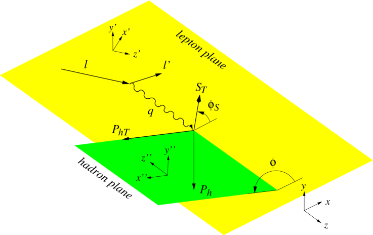
Figure 1: Kinematics of the process (1) in the target rest frame. $\mbox{\boldmath{$P$}}_{hT}$ and $\mbox{\boldmath{$S$}}_{T}$ respectively are the components of $\mbox{\boldmath{$P$}}_{h}$ and $S$ perpendicular to $q$. (The target spin vector $S$ is not shown.) $\phi$ and $\phi_{S}$ respectively are the azimuthal angles of $\mbox{\boldmath{$P$}}_{h}$ and $S$ in the coordinate system with axes $x$, $y$, $z$, in accordance with the Trento conventions [7].

To transform between the different target polarization states, we find it useful to introduce two coordinate systems $C$ and $C^{\prime}$ in the target rest frame, with respective axes $x$, $y$, $z$ and $x^{\prime}$, $y^{\prime}$, $z^{\prime}$ as shown in Figs. 1 and 2. The $z$ axis points along $q$, whereas the $z^{\prime}$ axis points along $l$. The $x$ axis and the $x^{\prime}$ axis are chosen such that $\mbox{\boldmath{$l$}}^{\prime}$ lies in the $x$-$z$ and the $x^{\prime}$-$z^{\prime}$ plane and has a positive $x$ and $x^{\prime}$ component. The $y$ and $y^{\prime}$ axes coincide. The two coordinate systems $C$ and $C^{\prime}$ are related via a rotation about the $y$ axis by the angle $\theta$ between $q$ and $l$. In terms of invariants we have

$$\sin\theta=\gamma\,\sqrt{\frac{1-y-\frac{1}{4}y^{2}\gamma^{2}}{1+\gamma^{2}}},\qquad\qquad\gamma=2x_{B}M_{p}/Q,$$ (2)

where $M_{p}$ is the proton mass. In deep inelastic kinematics $\gamma$ is small, and so is $\sin\theta\approx\gamma\sqrt{1-y\rule{0.0pt}{7.5pt}}$. Note for instance that $\gamma^{2}$ is the parameter controlling the size of target mass corrections in inclusive DIS [6].

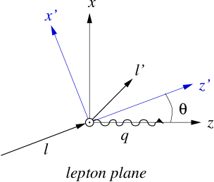
Figure 2: The lepton plane in the target rest frame. The $y$ and $y^{\prime}$ axes coincide and point out of the paper plane.

We parameterize the target spin vector $S$ in the two coordinate systems by

$$\mbox{\boldmath{$S$}}\,\stackrel{{\scriptstyle C}}{{=}}\,\left(\begin{array}[]{c}S_{T}\cos\phi_{S}\\ S_{T}\sin\phi_{S}\\ -S_{L}\end{array}\right),\qquad\qquad\mbox{\boldmath{$S$}}\,\stackrel{{\scriptstyle C^{\prime}}}{{=}}\,\left(\begin{array}[]{c}P_{T}\cos\psi\\ P_{T}\sin\psi\\ -P_{L}\end{array}\right),$$ (3)

so that $P_{L}$, $P_{T}$ specify longitudinal and transverse polarization relative to the lepton beam direction, and $S_{L}$, $S_{T}$ longitudinal and transverse polarization relative to the virtual photon direction. Likewise, $\psi$ is the azimuthal angle of the target spin around the lepton beam direction, whereas $\phi_{S}$ is the corresponding azimuthal angle around the virtual photon direction. $P_{L}$ and $S_{L}$ are between $-1$ and $1$, and $P_{T}$ and $S_{T}$ are between 0 and 1. The sign convention for the longitudinal case is such that $P_{L}=+1$ and $S_{L}=+1$ correspond to a right-handed proton in the $\ell p$ and $\gamma^{*}p$ center of mass, respectively. The values of $P_{L}$ and $P_{T}$ are determined by the experimental setup, whereas $S_{L}$ and $S_{T}$ depend on the kinematics of an individual event. The rotation from $C$ to $C^{\prime}$ readily gives

$$S_{T}\cos\phi_{S} = \cos\theta\,P_{T}\cos\psi-\sin\theta\,P_{L},$$

$$S_{T}\sin\phi_{S} = P_{T}\sin\psi,$$

$$S_{L} = \sin\theta\,P_{T}\cos\psi+\cos\theta\,P_{L}.$$ (4)

We remark that, although we work in the target rest frame, our results can readily be applied to a polarized $\ell p$ collider, whose laboratory frame is obtained from the target rest frame by a boost along the lepton beam momentum. $P_{L}$ and $P_{T}$ then give the longitudinal and transverse polarization of the proton beam with respect to the beam axis.

2.1 Longitudinal polarization with respect to the lepton beam

We have $P_{T}=0$, so that

$$S_{L}=\cos\theta\,P_{L},\qquad\qquad S_{T}\cos\phi_{S}=-\sin\theta\,P_{L},\qquad\qquad S_{T}\sin\phi_{S}=0.$$ (5)

If we allow $S_{T}$ to be negative, so that $(S_{T},\phi_{S})$ and $(-S_{T},\phi_{S}+\pi)$ are equivalent, the second and third relation can be written more simply as $S_{T}=-\sin\theta\,P_{L}$ and $\phi_{S}=0$.

2.2 Transverse polarization with respect to the lepton beam

With $P_{L}=0$ we find

$$S_{T}\cos\phi_{S}=\cos\theta\,P_{T}\cos\psi,\qquad S_{T}\sin\phi_{S}=P_{T}\sin\psi,\qquad S_{L}=\sin\theta\,P_{T}\cos\psi.$$ (6)

It turns out that the expression for the cross section in the next sections are considerably simpler when written in terms of the angle $\phi_{S}$ instead of $\psi$. We can use the relations (6) to obtain

$$\sin\psi=\frac{\cos\theta\,\sin\phi_{S}}{\sqrt{1-\sin^{2}\!\theta\,\sin^{2}\!\phi_{S}}},\qquad\qquad\cos\psi=\frac{\cos\phi_{S}}{\sqrt{1-\sin^{2}\!\theta\,\sin^{2}\!\phi_{S}}}$$ (7)

and, inserting this into the same relations, finally have

$$S_{T}=\frac{\cos\theta}{\sqrt{1-\sin^{2}\!\theta\,\sin^{2}\!\phi_{S}}}\,P_{T},\qquad\qquad S_{L}=\frac{\sin\theta\,\cos\phi_{S}}{\sqrt{1-\sin^{2}\!\theta\,\sin^{2}\!\phi_{S}}}\,P_{T}.$$ (8)

The phase space element is however simpler in terms of $\psi$, which describes the azimuthal distribution of the scattered lepton around the beam axis, with the reference direction provided by the target spin. Namely, we have

$$\frac{d^{3}l^{\prime}}{2l^{\prime 0}}=\frac{y}{4x_{B}}\,dx_{B}\,dQ^{2}\,d\psi=\frac{y}{4x_{B}}\,dx_{B}\,dQ^{2}\,d\phi_{S}\,\frac{\cos\theta}{1-\sin^{2}\!\theta\,\sin^{2}\!\phi_{S}}.$$ (9)

The transformation from $d\psi$ to $d\phi_{S}$ introduces an explicit $\phi_{S}$ dependence. In deep inelastic kinematics, one has however $d\psi\approx d\phi_{S}$ up to corrections of order $\gamma^{2}$.

2.3 Cross section and asymmetries

The dependence of the $\ell p$ cross section on the target polarization is at most linear in the spin vector $S$. This follows from the superposition principle and becomes for instance explicit in the spin density matrix formalism used in the next section. For an unpolarized lepton beam we can therefore write $d\sigma/(dx_{B}\,dQ^{2}\,d\phi\,d\psi)=a_{0}+\mbox{\boldmath{$S$}}\cdot\mbox{\boldmath{$a$}}$, where $a_{0}$ and $a$ only depend on the four-momenta of the reaction (1) but not on the target spin. Expressing the vectors in our coordinate system $C$ we have

$$\frac{d\sigma}{dx_{B}\,dQ^{2}\,d\phi\,d\psi}=a_{0}+S_{T}\cos\phi_{S}\,a_{1}+S_{T}\sin\phi_{S}\,a_{2}-S_{L}a_{3},$$ (10)

where the $a_{i}$ depend on $x_{B}$, $y$, $Q^{2}$ and $\phi$ but not on $\phi_{S}$ or $\psi$. With (5) and (8) we have

$$\frac{1}{2\pi}\,\frac{d\sigma}{dx_{B}\,dQ^{2}\,d\phi}\,\Bigg{|}_{P_{T}=0} = a_{0}-P_{L}\sin\theta\,a_{1}-P_{L}\cos\theta\,a_{3},$$

$$\frac{d\sigma}{dx_{B}\,dQ^{2}\,d\phi\,d\phi_{S}}\,\Bigg{|}_{P_{L}=0} = \frac{\cos\theta}{1-\sin^{2}\!\theta\,\sin^{2}\!\phi_{S}}$$ (11)

$$\times \Bigg{[}\,a_{0}+P_{T}\,\frac{\cos\theta\cos\phi_{S}\,a_{1}+\cos\theta\sin\phi_{S}\,a_{2}-\sin\theta\cos\phi_{S}\,a_{3}}{\sqrt{1-\sin^{2}\!\theta\,\sin^{2}\!\phi_{S}}}\,\Bigg{]},$$

where in the first relation we have integrated over $\psi$ and in the second one we have used (9) to trade $d\psi$ for $d\phi_{S}$.

It is often useful to express the spin dependence of a process through asymmetries. We define asymmetries for longitudinal and transverse target polarization with respect to the lepton beam

$$A_{UL}^{\ell} = \frac{d\sigma(P_{L}=+1)-d\sigma(P_{L}=-1)}{d\sigma(P_{L}=+1)+d\sigma(P_{L}=-1)}\;\Bigg{|}_{P_{T}=0}\,,$$

$$A_{UT}^{\ell}(\phi_{S}) = \frac{d\sigma(\phi_{S})-d\sigma(\phi_{S}+\pi)}{d\sigma(\phi_{S})+d\sigma(\phi_{S}+\pi)}\;\Bigg{|}_{P_{T}=1,P_{L}=0}$$ (12)

in accordance with the Trento conventions [7]. The subscript $U$ indicates an unpolarized lepton beam, and for better legibility we have not displayed the dependence of the cross sections and asymmetries on other kinematical variables $\phi$, $x_{B}$, $Q^{2}$, etc. These asymmetries can be directly measured in experiment, whereas their counterparts for longitudinal and transverse target polarization with respect to the virtual photon direction

$$A_{UL}^{\gamma^{*}} = \frac{d\sigma(S_{L}=+1)-d\sigma(S_{L}=-1)}{d\sigma(S_{L}=+1)+d\sigma(S_{L}=-1)}\;\Bigg{|}_{S_{T}=0}\,,$$

$$A_{UT}^{\gamma^{*}}(\phi_{S}) = \frac{d\sigma(\phi_{S})-d\sigma(\phi_{S}+\pi)}{d\sigma(\phi_{S})+d\sigma(\phi_{S}+\pi)}\;\Bigg{|}_{S_{T}=1,S_{L}=0}$$ (13)

are more natural to describe the physics of the $\gamma^{*}p$ subprocess. From (10) and (2.3) we readily obtain the transformation between the two types of asymmetries,

$$A_{UL}^{\ell} = \cos\theta\,A_{UL}^{\gamma^{*}}-\sin\theta\,A_{UT}^{\gamma^{*}}(0)\,,$$

$$A_{UT}^{\ell}(\phi_{S}) = \frac{\cos\theta\,A_{UT}^{\gamma^{*}}(\phi_{S})+\sin\theta\,\cos\phi_{S}\,A_{UL}^{\gamma^{*}}\rule[-3.99994pt]{0.0pt}{10.00002pt}}{\sqrt{1-\sin^{2}\!\theta\,\sin^{2}\!\phi_{S}}}$$ (14)

and its inverse

$$A_{UL}^{\gamma^{*}} = \cos\theta\,A_{UL}^{\ell}+\sin\theta\,A_{UT}^{\ell}(0)\,,$$

$$A_{UT}^{\gamma^{*}}(\phi_{S}) = \frac{\sqrt{1-\sin^{2}\!\theta\,\sin^{2}\!\phi_{S}}\;A_{UT}^{\ell}(\phi_{S})}{\cos\theta}-\sin\theta\,\cos\phi_{S}\,\Big{(}A_{UL}^{\ell}+\tan\theta\,A_{UT}^{\ell}(0)\Big{)}$$ (15)

$$= \cos\phi_{S}\,\Big{(}\cos\theta\,A_{UT}^{\ell}(0)-\sin\theta\,A_{UL}^{\ell}\,\Big{)}+\sin\phi_{S}\,A_{UT}^{\ell}({\textstyle\frac{1}{2}}\pi)\,.$$

An experiment having both longitudinal and transverse target polarization can hence uniquely reconstruct the asymmetries $A_{UL}^{\gamma^{*}}$ and $A_{UT}^{\gamma^{*}}(\phi_{S})$. To determine $A_{UT}^{\ell}(\phi_{S})$ at $\phi_{S}=0$ or $\phi_{S}={\textstyle\frac{1}{2}}\pi$ one can of course use data for all $\phi_{S}$, given that

$$A_{UT}^{\ell}(\phi_{S})=\frac{\cos\phi_{S}\,A_{UT}^{\ell}(0)+\cos\theta\,\sin\phi_{S}\,A_{UT}^{\ell}({\textstyle\frac{1}{2}}\pi)\rule[-3.99994pt]{0.0pt}{10.00002pt}}{\sqrt{1-\sin^{2}\!\theta\,\sin^{2}\!\phi_{S}}}$$ (16)

according to (2.3). Notice that the transformations (2.3) and (2.3) require $\theta$ to be fixed, which implies that the cross sections in (2.3) and (2.3) have to be differential in both $x_{B}$ and $Q^{2}$ (which also fixes $y$ for a given c.m. energy of the $\ell p$ collision). If the measured cross sections are integrated over wider bins in $x_{B}$ and $Q^{2}$, the transformations can only be done approximately, with an average value of $\theta$.

Our results generalize straightforwardly to the case of a longitudinally polarized lepton beam. The relations (10) and (2.3) then hold separately for right- and left-handed beam polarization with coefficients $a_{i}^{\rightarrow}$ and $a_{i}^{\leftarrow}$ . (Since we neglect the lepton mass, the lepton helicity is a good quantum number and frame independent.) Writing $d\sigma^{\rightarrow}$ and $d\sigma^{\leftarrow}$ for the respective cross section with a right-handed and left-handed lepton beam, we introduce double spin asymmetries

$$A_{LL}^{\ell} = \frac{d\sigma^{\rightarrow}(P_{L}=+1)-d\sigma^{\rightarrow}(P_{L}=-1)-d\sigma^{\leftarrow}(P_{L}=+1)+d\sigma^{\leftarrow}(P_{L}=-1)}{d\sigma^{\rightarrow}(P_{L}=+1)+d\sigma^{\rightarrow}(P_{L}=-1)+d\sigma^{\leftarrow}(P_{L}=+1)+d\sigma^{\leftarrow}(P_{L}=-1)}\;\Bigg{|}_{P_{T}=0}\,,$$

$$A_{LT}^{\ell}(\phi_{S}) = \frac{d\sigma^{\rightarrow}(\phi_{S})-d\sigma^{\rightarrow}(\phi_{S}+\pi)-d\sigma^{\leftarrow}(\phi_{S})+d\sigma^{\leftarrow}(\phi_{S}+\pi)}{d\sigma^{\rightarrow}(\phi_{S})+d\sigma^{\rightarrow}(\phi_{S}+\pi)+d\sigma^{\leftarrow}(\phi_{S})+d\sigma^{\leftarrow}(\phi_{S}+\pi)}\;\Bigg{|}_{P_{T}=1,P_{L}=0}$$ (17)

and their analogs $A_{LL}^{\gamma^{*}}$ and $A_{LT}^{\gamma^{*}}(\phi_{S})$, with $(P_{L},P_{T})$ replaced by $(S_{L},S_{T})$. One then has relations like (2.3), (2.3) and (16) with the subscript $U$ replaced by $L$.

3 From $\ell p$ to $\gamma^{*}p$ cross sections

In the previous section we have given the transformation between target polarization defined with respect to either the direction of $l$ or the direction of $\mbox{\boldmath{$q$}}=\mbox{\boldmath{$l$}}-\mbox{\boldmath{$l$}}^{\prime}$. We have not actually used that $q$ is the momentum of a virtual photon which is radiated off the lepton beam and absorbed by the target proton. We now use this, which will in particular allow us to make explicit the interplay between the azimuthal angles $\phi$ and $\phi_{S}$. The discussion in this chapter holds for processes like SIDIS and exclusive meson production, but not for DVCS (see Sect. 8).

Our evaluation of the $\ell p$ cross section closely follows the steps detailed in Sect. 3 of [8] for an unpolarized target. A reader not interested in the derivation may directly go to the result (29). To describe the $\gamma^{*}p$ subprocess we use a coordinate system $C^{\prime\prime}$ with axes $x^{\prime\prime}$, $y^{\prime\prime}$, $z^{\prime\prime}$ as shown in Fig. 1. The $z^{\prime\prime}$ axis points opposite to $q$ and the $x^{\prime\prime}$ axis is chosen such that $\mbox{\boldmath{$P$}}_{h}$ lies in the $x^{\prime\prime}$-$z^{\prime\prime}$ plane and has a positive $x^{\prime\prime}$ component. In this coordinate system the proton spin vector reads

$$\mbox{\boldmath{$S$}}\,\stackrel{{\scriptstyle C^{\prime\prime}}}{{=}}\,\left(\begin{array}[]{c}S_{T}\cos(\phi-\phi_{S})\\ S_{T}\sin(\phi-\phi_{S})\\ S_{L}\end{array}\right)$$ (18)

and the spin density matrix of the target [9] can be written as

$$\rho_{ji}\,=\,\frac{1}{2}\Big{[}\delta_{ji}+\mbox{\boldmath{$S$}}\cdot\mbox{\boldmath{$\sigma$}}_{ji}\Big{]}\;\stackrel{{\scriptstyle C^{\prime\prime}}}{{=}}\;\frac{1}{2}\left(\begin{array}[]{cc}1+S_{L}&S_{T}\exp[-i(\phi-\phi_{S})]\\ S_{T}\exp[i(\phi-\phi_{S})]&1-S_{L}\end{array}\right)$$ (19)

in a basis of polarization states specified by two-component spinors

$$\chi_{+\frac{1}{2}}=\left(\begin{array}[]{c}1\\ 0\end{array}\right),\qquad\qquad\chi_{-\frac{1}{2}}=\left(\begin{array}[]{c}0\\ 1\end{array}\right).$$ (20)

These states respectively correspond to definite spin projection $+\frac{1}{2}$ and $-\frac{1}{2}$ along the $z^{\prime\prime}$ axis, and to right- and left-handed proton helicity in the $\gamma^{*}p$ center of mass. The components of $\sigma$ in (19) are the Pauli matrices. As is well known, the cross section can be written as

$$d\sigma(\ell p\to\ell hX)\propto L^{\nu\mu}W_{\mu\nu}\;\frac{d^{3}l^{\prime}}{2l^{\prime 0}}\,\frac{d^{3}P_{h}}{2P_{h}^{0}},$$ (21)

with a proportionality factor depending on $x_{B}$, $y$ and $Q^{2}$. The leptonic tensor reads

$$L^{\nu\mu}=l^{\prime\nu}l^{\mu}+l^{\nu}l^{\prime\mu}-(l^{\prime}\cdot l)\,g^{\nu\mu}+iP_{\ell}\,\epsilon^{\nu\mu\alpha\beta}q_{\alpha}l_{\beta}$$ (22)

with the convention $\epsilon_{0123}=1$ and the lepton beam polarization $P_{\ell}$ defined such that $P_{\ell}=+1$ corresponds to a purely right-handed and $P_{\ell}=-1$ to a purely left-handed beam. The hadronic tensor is given by

$$W_{\mu\nu}=\sum_{ij}\rho_{ji}\sum_{X}\delta^{(4)}(P^{\prime}+P_{h}-P-q)\sum_{\rm spins}\langle p(i)|J_{\mu}(0)|hX\rangle\,\langle hX|J_{\nu}(0)|p(j)\rangle,$$ (23)

where $J_{\mu}$ is the electromagnetic current. $\sum_{X}$ denotes the integral over the momenta of all hadrons in $X$, and also the sum over their number if $X$ is an inclusive system. There are further sums $\sum_{ij}$ over target spin states $i,j=\pm\frac{1}{2}$ and $\sum_{\rm spins}$ over all polarizations in the hadronic final state $hX$. We now introduce polarization vectors $\epsilon_{m}$ for definite helicity $m$ of the virtual photon,

$$\epsilon_{0}^{\mu} = \frac{1}{Q\sqrt{1+\gamma^{2}}}\,\Big{(}q^{\mu}+\frac{Q^{2}}{P\cdot q}\,P^{\mu}\Big{)},$$

$$\epsilon_{+1} = \frac{1}{\sqrt{2}}\,(0,-1,i,0),\qquad\qquad\epsilon_{-1}\;=\>\frac{1}{\sqrt{2}}\,(0,1,i,0),$$ (24)

with $\gamma$ defined in (2) and the components of $\epsilon_{\pm 1}$ given in coordinate system $C^{\prime\prime}$. As shown in [8], the leptonic tensor $L^{\nu\mu}$ can be expressed as a linear combination of terms $\epsilon^{\nu}_{n}\epsilon^{\mu*}_{m}$. Up to a global factor the expansion coefficients form the spin density matrix of the virtual photon. They depend on $P_{\ell}$, on $Q^{2}$, on the usual ratio of longitudinal and transverse photon flux

$$\varepsilon=\frac{1-y-\frac{1}{4}y^{2}\gamma^{2}}{1-y+\frac{1}{2}y^{2}+\frac{1}{4}y^{2}\gamma^{2}}\,,$$ (25)

and on the azimuthal angle $\phi$. The contraction $L^{\nu\mu}W_{\mu\nu}$ can then be written in terms of quantities

$$\rule[-11.99998pt]{0.0pt}{32.00002pt}\sigma_{mn}=\sum_{ij}\rho_{ji}^{\phantom{m}}\,\sigma^{ij}_{mn}\propto\int dt\,dM_{X}^{2}\,(\epsilon^{\mu*}_{m}W_{\mu\nu}^{\phantom{*}}\,\epsilon^{\nu}_{n}),$$ (26)

where the $x_{B}$ and $Q^{2}$ dependent proportionality factor is chosen such that $\sigma_{mm}$ is the $\gamma^{*}p$ cross section for photon helicity $m$ with Hand’s convention for the virtual photon flux. In (26) we have integrated over the invariant momentum transfer $t=(P-P^{\prime})^{2}=(P_{h}-q)^{2}$ and over the invariant mass $M_{X}^{2}=P^{\prime 2}$ of the system $X$. The $\sigma^{ij}_{mn}$ are polarized photoabsorption cross sections or interference terms, given by

$$\sigma^{ij}_{mn}(x_{B},Q^{2})\propto\int dt\,dM_{X}^{2}\,\sum_{X}\delta^{(4)}(P^{\prime}+P_{h}-P-q)\sum_{\rm spins}\Big{(}\mathcal{A}^{i}_{m}\Big{)}^{*}\mathcal{A}^{j}_{n}$$ (27)

in terms of the amplitudes $\mathcal{A}^{i}_{m}$ for the subprocess $\gamma^{*}p\to hX$ with proton polarization $i$ and photon polarization $m$. Changing the basis of spin states one can rewrite interference terms as linear combinations of cross sections, as shown in App. A. We have defined our polarization states for protons and photons in the coordinate system $C^{\prime\prime}$, whose axes are specified with reference only to the momenta of the $\gamma^{*}p$ process, but not to the lepton momenta or to the proton polarization. Therefore $\sigma^{ij}_{mn}$ depends on the kinematical variables $x_{B}$ and $Q^{2}$, whereas the dependence on $\varepsilon$ and $\phi$ is contained in $L^{\nu\mu}$ and the dependence on $S_{T}$, $S_{L}$ and $\phi_{S}$ in $\rho_{ji}$. From hermiticity and parity invariance we have relations $\sigma_{nm}^{\phantom{*}}=\sigma_{mn}^{*}$ and

$$\rule[-11.99998pt]{0.0pt}{32.00002pt}\sigma^{ji}_{nm}=(\sigma^{ij}_{mn})^{*},\qquad\qquad\sigma^{-i-j}_{-m-n}=(-1)^{m-n-i+j}\,\sigma^{ij}_{mn}$$ (28)

with $m,n=0,+1,-1$ and $i,j=+\frac{1}{2},-\frac{1}{2}$. They imply that $\sigma_{00}^{+-}$, $\sigma_{+-}^{+-}$ and $\sigma_{+-}^{-+}$ are purely imaginary, whereas other interference terms have both real and imaginary parts. Using these relations and closely following the steps of the derivation in [8] we obtain our master formula

$$\Bigg{[}\frac{\alpha_{\rm em}}{8\pi^{3}}\,\frac{y^{2}}{1-\varepsilon}\,\frac{1-x_{B}}{x_{B}}\,\frac{1}{Q^{2}}\Bigg{]}^{-1}\frac{d\sigma}{dx_{B}\,dQ^{2}\,d\phi\,d\psi}$$ (29)

$$= \frac{1}{2}\Big{(}\sigma_{++}^{++}+\sigma_{++}^{--}\Big{)}+\varepsilon\sigma_{00}^{++}-\varepsilon\cos(2\phi)\,\mathrm{Re}\,\sigma_{+-}^{++}-\sqrt{\varepsilon(1+\varepsilon)}\,\cos\phi\,\mathrm{Re}\,(\sigma_{+0}^{++}+\sigma_{+0}^{--})\phantom{\Bigg{[}\Bigg{]}}$$

$${}-P_{\ell}\,\sqrt{\varepsilon(1-\varepsilon)}\,\sin\phi\,\mathrm{Im}\,(\sigma_{+0}^{++}+\sigma_{+0}^{--})\phantom{\Bigg{[}\Bigg{]}}$$

$${}-S_{L}\,\Bigg{[}\varepsilon\sin(2\phi)\,\mathrm{Im}\,\sigma_{+-}^{++}+\sqrt{\varepsilon(1+\varepsilon)}\,\sin\phi\,\mathrm{Im}\,(\sigma_{+0}^{++}-\sigma_{+0}^{--})\Bigg{]}$$

$${}+S_{L}P_{\ell}\,\Bigg{[}\,\sqrt{1-\varepsilon^{2}}\;\frac{1}{2}\Big{(}\sigma_{++}^{++}-\sigma_{++}^{--}\Big{)}-\sqrt{\varepsilon(1-\varepsilon)}\,\cos\phi\,\mathrm{Re}\,(\sigma_{+0}^{++}-\sigma_{+0}^{--})\Bigg{]}$$

$${}-S_{T}\,\Bigg{[}\sin(\phi-\phi_{S})\,\mathrm{Im}\,(\sigma_{++}^{+-}+\varepsilon\sigma_{00}^{+-})+\frac{\varepsilon}{2}\sin(\phi+\phi_{S})\,\mathrm{Im}\,\sigma_{+-}^{+-}+\frac{\varepsilon}{2}\sin(3\phi-\phi_{S})\,\mathrm{Im}\,\sigma_{+-}^{-+}$$

$$\hskip 20.00003pt{}+\sqrt{\varepsilon(1+\varepsilon)}\,\sin\phi_{S}\,\mathrm{Im}\,\sigma_{+0}^{+-}+\sqrt{\varepsilon(1+\varepsilon)}\,\sin(2\phi-\phi_{S})\,\mathrm{Im}\,\sigma_{+0}^{-+}\Bigg{]}$$

$${}+S_{T}P_{\ell}\,\Bigg{[}\sqrt{1-\varepsilon^{2}}\,\cos(\phi-\phi_{S})\,\mathrm{Re}\,\sigma_{++}^{+-}$$

$$\hskip 30.00005pt{}-\sqrt{\varepsilon(1-\varepsilon)}\,\cos\phi_{S}\,\mathrm{Re}\,\sigma_{+0}^{+-}-\sqrt{\varepsilon(1-\varepsilon)}\,\cos(2\phi-\phi_{S})\,\mathrm{Re}\,\sigma_{+0}^{-+}\Bigg{]}.$$

For the sake of legibility we have labeled the target spin states by $\pm$ instead of $\pm\frac{1}{2}$. In the following we will also use the common notation

$$\sigma_{T}={\textstyle\frac{1}{2}}(\sigma_{++}^{++}+\sigma_{++}^{--}),\qquad\qquad\sigma_{L}=\sigma_{00}^{++}$$ (30)

for the transverse and longitudinal $\gamma^{*}p$ cross sections. The dependence of the $\ell p$ cross section on $\varepsilon$ and on the angles $\phi$ and $\phi_{S}$ (or $\psi$ as explained in Sect. 2.2) is fully explicit in (29).

Relations analogous to (28) and (29) hold for cross sections and interference terms that are differential in $M_{X}^{2}$ and $t$, or equivalently in $M_{X}^{2}$ and $\mbox{\boldmath{$P$}}_{hT}^{2}$, where $\mbox{\boldmath{$P$}}_{hT}^{\phantom{2}}$ is the transverse component of the hadron momentum with respect to the virtual photon momentum (see Fig. 1). Let us analyze the behavior of the different interference terms in the region of small $\mbox{\boldmath{$P$}}_{hT}$. To this end we go to the $\gamma^{*}p$ center of mass and consider the amplitudes for $\gamma^{*}p\to hX$ as a function of the scattering angle $\Theta$ between $h$ and $\gamma^{*}$. For semi-inclusive processes, we can choose the set of states $X$ to be summed over in the cross section such that the system $X$ has definite total spin $j_{X}$ and definite spin projection $m_{X}$ along its momentum. For exclusive processes we simply choose helicity states of the single hadron $X$. Also taking states with definite helicity $m_{h}$ of the hadron $h$, we can perform a partial-wave decomposition of the $\gamma^{*}p$ scattering amplitude (see e.g. [9]):

$$\mathcal{A}_{m}^{i}(j_{X},m_{X},m_{h};\Theta)=\sum_{J}a_{m}^{i}(j_{X},m_{X},m_{h};J)\;d^{J}_{i-m,\,m_{X}-m_{h}}(\Theta).$$ (31)

For $\Theta\to 0$ the rotation functions follow the behavior $d^{J}_{\mu,\,\mu^{\prime}}(\Theta)\sim\Theta^{|\mu-\mu^{\prime}|}$. In the product $(\mathcal{A}^{i}_{m})^{*}\mathcal{A}^{j}_{n}$ we thus have a sum over terms which behave like $\Theta$ to the power $|i-m-m_{X}+m_{h}|+|j-n-m_{X}+m_{h}|\geq|i-m-j+n|$. Since $\Theta\sim|\mbox{\boldmath{$P$}}_{hT}|$ for small $\Theta$, we finally obtain a power behavior like

$$\frac{d\sigma^{ij}_{mn}}{d\mbox{\boldmath{$P$}}_{hT}^{2}}\sim|\mbox{\boldmath{$P$}}_{hT}|^{|m-n-i+j|}\qquad\qquad\mbox{for~{}}\mbox{\boldmath{$P$}}_{hT}\to 0,$$ (32)

or like a higher power of $|\mbox{\boldmath{$P$}}_{hT}|$. Applying this to our cross section formula (29) we find the simple rule that terms coming with an angular dependence $\cos(M\phi+N\phi_{S})$ or $\sin(M\phi+N\phi_{S})$ behave like $d\sigma_{mn}^{ij}/(d\mbox{\boldmath{$P$}}_{hT}^{2})\sim|\mbox{\boldmath{$P$}}_{hT}|^{M}$ or like a higher power, where $M=0,1,2,3$ and $N=-1,0,1$.

Using the transformations (5) and (8) we obtain from (29) the cross sections for definite target polarization with respect to the lepton beam,

$$\Bigg{[}\frac{\alpha_{\rm em}}{4\pi^{2}}\,\frac{y^{2}}{1-\varepsilon}\,\frac{1-x_{B}}{x_{B}}\,\frac{1}{Q^{2}}\Bigg{]}^{-1}\frac{d\sigma}{dx_{B}\,dQ^{2}\,d\phi}\;\Bigg{|}_{P_{T}=0}=\mbox{terms independent of $P_{L}$}$$ (33)

$$- P_{L}\,\Bigg{[}\sin\phi\,\Big{(}\cos\theta\sqrt{\varepsilon(1+\varepsilon)}\,\mathrm{Im}\,(\sigma_{+0}^{++}-\sigma_{+0}^{--})-\sin\theta\,\mathrm{Im}\,(\sigma_{++}^{+-}+\varepsilon\sigma_{00}^{+-})-\sin\theta\,\frac{\varepsilon}{2}\,\mathrm{Im}\,\sigma_{+-}^{+-}\Big{)}$$

$$\hskip 8.00003pt{}+\sin(2\phi)\,\Big{(}\cos\theta\,\varepsilon\,\mathrm{Im}\,\sigma_{+-}^{++}-\sin\theta\,\sqrt{\varepsilon(1+\varepsilon)}\,\mathrm{Im}\,\sigma_{+0}^{-+}\Big{)}$$

$$\hskip 8.00003pt{}-\sin(3\phi)\,\sin\theta\,\frac{\varepsilon}{2}\,\mathrm{Im}\,\sigma_{+-}^{-+}\Bigg{]}$$

$$+ P_{L}P_{\ell}\,\Bigg{[}\cos\theta\sqrt{1-\varepsilon^{2}}\;\frac{1}{2}(\sigma_{++}^{++}-\sigma_{++}^{--})+\sin\theta\sqrt{\varepsilon(1-\varepsilon)}\,\mathrm{Re}\,\sigma_{+0}^{+-}$$

$$\hskip 20.00003pt{}-\cos\phi\,\Big{(}\cos\theta\sqrt{\varepsilon(1-\varepsilon)}\,\mathrm{Re}\,(\sigma_{+0}^{++}-\sigma_{+0}^{--})+\sin\theta\sqrt{1-\varepsilon^{2}}\,\mathrm{Re}\,\sigma_{++}^{+-}\Big{)}$$

$$\hskip 20.00003pt{}+\cos(2\phi)\,\sin\theta\sqrt{\varepsilon(1-\varepsilon)}\,\mathrm{Re}\,\sigma_{+0}^{-+}\Bigg{]}$$

for longitudinal and

$$\Bigg{[}\frac{\cos\theta}{1-\sin^{2}\!\theta\,\sin^{2}\!\phi_{S}}\Bigg{]}^{-1}\,\Bigg{[}\frac{\alpha_{\rm em}}{8\pi^{3}}\,\frac{y^{2}}{1-\varepsilon}\,\frac{1-x_{B}}{x_{B}}\,\frac{1}{Q^{2}}\Bigg{]}^{-1}\frac{d\sigma}{dx_{B}\,dQ^{2}\,d\phi\,d\phi_{S}}\;\Bigg{|}_{P_{L}=0}$$ (34)

$$= P_{T}$$ terms independent of

$$- \frac{P_{T}}{\sqrt{1-\sin^{2}\!\theta\,\sin^{2}\!\phi_{S}}}\,\Bigg{[}\sin\phi_{S}\,\cos\theta\sqrt{\varepsilon(1+\varepsilon)}\,\mathrm{Im}\,\sigma_{+0}^{+-}$$

$$\hskip 81.00018pt{}+\sin(\phi-\phi_{S})\,\Big{(}\cos\theta\,\mathrm{Im}\,(\sigma_{++}^{+-}+\varepsilon\sigma_{00}^{+-})+\frac{1}{2}\sin\theta\sqrt{\varepsilon(1+\varepsilon)}\,\mathrm{Im}\,(\sigma_{+0}^{++}-\sigma_{+0}^{--})\Big{)}$$

$$\hskip 81.00018pt{}+\sin(\phi+\phi_{S})\,\Big{(}\cos\theta\,\frac{\varepsilon}{2}\,\mathrm{Im}\,\sigma_{+-}^{+-}+\frac{1}{2}\sin\theta\sqrt{\varepsilon(1+\varepsilon)}\,\mathrm{Im}\,(\sigma_{+0}^{++}-\sigma_{+0}^{--})\Big{)}$$

$$\hskip 81.00018pt{}+\sin(2\phi-\phi_{S})\,\Big{(}\cos\theta\sqrt{\varepsilon(1+\varepsilon)}\,\mathrm{Im}\,\sigma_{+0}^{-+}+\frac{1}{2}\sin\theta\,\varepsilon\,\mathrm{Im}\,\sigma_{+-}^{++}\Big{)}$$

$$\hskip 81.00018pt{}+\sin(2\phi+\phi_{S})\,\frac{1}{2}\sin\theta\,\varepsilon\,\mathrm{Im}\,\sigma_{+-}^{++}$$

$$\hskip 81.00018pt{}+\sin(3\phi-\phi_{S})\,\cos\theta\,\frac{\varepsilon}{2}\,\mathrm{Im}\,\sigma_{+-}^{-+}\,\Bigg{]}$$

$$- \frac{P_{T}P_{\ell}}{\sqrt{1-\sin^{2}\!\theta\,\sin^{2}\!\phi_{S}}}\,\Bigg{[}\cos\phi_{S}\,\Big{(}\cos\theta\sqrt{\varepsilon(1-\varepsilon)}\,\mathrm{Re}\,\sigma_{+0}^{+-}-\sin\theta\sqrt{1-\varepsilon^{2}}\;\frac{1}{2}(\sigma_{++}^{++}-\sigma_{++}^{--})\Big{)}$$

$$\hskip 81.00018pt{}-\cos(\phi-\phi_{S})\,\Big{(}\cos\theta\sqrt{1-\varepsilon^{2}}\,\mathrm{Re}\,\sigma_{++}^{+-}-\frac{1}{2}\sin\theta\sqrt{\varepsilon(1-\varepsilon)}\,\mathrm{Re}\,(\sigma_{+0}^{++}-\sigma_{+0}^{--})\Big{)}$$

$$\hskip 81.00018pt{}+\cos(\phi+\phi_{S})\,\frac{1}{2}\sin\theta\sqrt{\varepsilon(1-\varepsilon)}\,\mathrm{Re}\,(\sigma_{+0}^{++}-\sigma_{+0}^{--})$$

$$\hskip 81.00018pt{}+\cos(2\phi-\phi_{S})\,\cos\theta\,\sqrt{\varepsilon(1-\varepsilon)}\,\mathrm{Re}\,\sigma_{+0}^{-+}\,\Bigg{]}$$

for transverse polarization. The terms independent of $P_{L}$ and $P_{T}$ are those given in the first two lines on the right-hand side of (29). Although the expressions for the experimentally accessible cross sections (33) and (34) are a little lengthy, they have a clear structure. Using the relations $\cos\phi_{S}\,\sin(n\phi)=\frac{1}{2}[\,\sin(n\phi+\phi_{S})+\sin(n\phi-\phi_{S})\,]$ and $\cos\phi_{S}\,\cos(n\phi)=\frac{1}{2}[\,\cos(n\phi+\phi_{S})+\cos(n\phi-\phi_{S})\,]$, we have written the cross sections such that the terms in each line can be experimentally separated by measuring the dependence on $\phi$ and (with transverse target polarization) on $\phi_{S}$. Different terms $\sigma_{mn}^{ij}(x_{B},Q^{2})$ multiplying the same function of $\phi$ and $\phi_{S}$ can be separated by the Rosenbluth technique, measuring at several $\ell p$ collision energies to get several values of $\varepsilon$ at the same $x_{B}$ and $Q^{2}$. A different possibility is to combine data with transverse and longitudinal target polarization. Here one can analyze a limited number of terms at a time:

1. The three combinations $\mathrm{Im}\,(\sigma_{+0}^{++}-\sigma_{+0}^{--})$, $\mathrm{Im}\,(\sigma_{++}^{+-}+\varepsilon\sigma_{00}^{+-})$ and $\mathrm{Im}\,\sigma_{+-}^{+-}$ can be separated by combined analysis of the $\sin\phi$ term in the longitudinal cross section (33) and the $\sin(\phi-\phi_{S})$ and $\sin(\phi+\phi_{S})$ terms in the transverse cross section (34). Further separation of $\mathrm{Im}\,\sigma_{++}^{+-}$ and $\mathrm{Im}\,\sigma_{00}^{+-}$ is only possible with the Rosenbluth method, as is the separation of the cross sections $\sigma_{T}$ and $\sigma_{L}$ in $\sigma_{T}+\varepsilon\sigma_{L}$. The terms just discussed are of particular physical interest, and we will come back to them in Sect. 5, 6 and 7.

2. The cross section difference $\sigma_{++}^{++}-\sigma_{++}^{--}$ and the interference term $\mathrm{Re}\,\sigma_{+0}^{+-}$ can be obtained by combined analysis of the $\phi$ independent terms in (33) and (34), i.e. by integrating over $\phi$ and forming double spin asymmetries for polarized beam and target. In this case, the transformation between asymmetries for target polarization with respect to the beam or to the virtual photon direction is well known from the measurement of the structure functions $g_{1}$ and $g_{2}$ in inclusive DIS. We give the relation between the notation usually employed in the literature and ours in App. B.

3. $\mathrm{Im}\,\sigma_{+-}^{++}$ and $\mathrm{Im}\,\sigma_{+0}^{-+}$ can be separated by measuring both the $\sin(2\phi)$ term in (33) and the $\sin(2\phi-\phi_{S})$ term in (34). $\mathrm{Im}\,\sigma_{+-}^{++}$ can also directly be obtained from the $\sin(2\phi+\phi_{S})$ term for transverse target polarization, where it is however suppressed by $\sin\theta$. The situation is analogous for the $\cos\phi$ term in (33) and the $\cos(\phi-\phi_{S})$ and $\cos(\phi+\phi_{S})$ terms in (34).

4. $\mathrm{Im}\,\sigma_{+-}^{-+}$ can either be extracted from the $\sin(3\phi-\phi_{S})$ term in the transverse cross section, or from the $\sin(3\phi)$ term in the longitudinal one, where it is however suppressed by $\sin\theta$. An analogous statement holds for the $\cos(2\phi-\phi_{S})$ term in (34) and the $\cos(2\phi)$ term in (33). Finally, the interference term $\mathrm{Im}\,\sigma_{+0}^{+-}$ only appears in the transverse cross section (34).

To conclude this section we take a closer look on azimuthal moments for transverse target polarization, which are given by

$$\langle w(\phi,\phi_{S})\,\rangle_{UT}^{\ell}=\frac{\int d\phi\,d\phi_{S}\,w(\phi,\phi_{S})\,[S(\phi,\phi_{S})-S(\phi,\phi_{S}+\pi)]\rule[-5.0pt]{0.0pt}{10.00002pt}}{\int d\phi\,d\phi_{S}\,[S(\phi,\phi_{S})+S(\phi,\phi_{S}+\pi)]\rule{0.0pt}{11.00008pt}}\;\Bigg{|}_{P_{T}=1,P_{L}=0}$$ (35)

and similarly for the double spin asymmetry with polarized beam and target. For brevity we have written $S(\phi,\phi_{S})=d\sigma/(dx_{B}\,dQ^{2}\,d\phi\,d\phi_{S})$ and not displayed the dependence on $x_{B}$, $y$ and $Q^{2}$. Without the $\phi_{S}$ dependence introduced by the global factor

$$f(\sin^{2}\!\phi_{S})=\frac{\cos\theta}{(1-\sin^{2}\!\theta\,\sin^{2}\!\phi_{S})^{3/2}\rule{0.0pt}{11.00008pt}}$$ (36)

in the $P_{T}$ dependent part of $S(\phi,\phi_{S})$, the moment of $w(\phi,\phi_{S})=2\sin(m\phi+\phi_{S})$ would directly project out the $\sin(m\phi+\phi_{S})$ term in the transverse cross section (34), where $m=0,\pm 1,\pm 2,-3$. Taking the effect of this term into account is straightforward, given that

$$\frac{1}{2\pi^{2}}\int_{0}^{2\pi}d\phi\int_{0}^{2\pi}d\phi_{S}\,f(\sin^{2}\!\phi_{S})\sin(n\phi+\phi_{S})\,\sin(m\phi+\phi_{S})$$ (37)

$$= \left\{\begin{array}[]{lll}{\displaystyle\frac{1}{\pi}\int_{0}^{2\pi}}d\phi_{S}\,f(\sin^{2}\!\phi_{S})\,\sin^{2}\!\phi_{S}&=1+\frac{5}{8}\sin^{2}\!\theta+O(\sin^{4}\!\theta)&\mbox{~{}for~{}}n=m=0,\\ {\displaystyle\frac{1}{2\pi}\int_{0}^{2\pi}}d\phi_{S}\,f(\sin^{2}\!\phi_{S})&=1+\frac{1}{4}\sin^{2}\!\theta+O(\sin^{4}\!\theta)&\mbox{~{}for~{}}n=m\neq 0,\\ {\displaystyle\frac{1}{2\pi}\int_{0}^{2\pi}}d\phi_{S}\,f(\sin^{2}\!\phi_{S})\,(2\sin^{2}\!\phi_{S}-1)&=\frac{3}{8}\sin^{2}\!\theta+O(\sin^{4}\!\theta)&\mbox{~{}for~{}}n=-m\neq 0,\end{array}\right.$$ (41)

$$\frac{1}{2\pi^{2}}\int_{0}^{2\pi}d\phi\int_{0}^{2\pi}d\phi_{S}\,f(\sin^{2}\!\phi_{S})\cos(n\phi+\phi_{S})\,\cos(m\phi+\phi_{S})$$ (45)

$$= \left\{\begin{array}[]{lll}{\displaystyle\frac{1}{\pi}\int_{0}^{2\pi}}d\phi_{S}\,f(\sin^{2}\!\phi_{S})\,\cos^{2}\phi_{S}&=1-\frac{1}{8}\sin^{2}\!\theta-O(\sin^{4}\!\theta)&\mbox{~{}for~{}}n=m=0,\\ {\displaystyle\frac{1}{2\pi}\int_{0}^{2\pi}}d\phi_{S}\,f(\sin^{2}\!\phi_{S})&=1+\frac{1}{4}\sin^{2}\!\theta+O(\sin^{4}\!\theta)&\mbox{~{}for~{}}n=m\neq 0,\\ {\displaystyle\frac{1}{2\pi}\int_{0}^{2\pi}}d\phi_{S}\,f(\sin^{2}\!\phi_{S})\,(2\cos^{2}\phi_{S}-1)&=-\frac{3}{8}\sin^{2}\!\theta-O(\sin^{4}\!\theta)&\mbox{~{}for~{}}n=-m\neq 0,\end{array}\right.$$

where for all other combinations of $m$ and $n$ the integrals are zero. For simplicity we have Taylor expanded the exact expressions, which are given by elliptic integrals. We see in particular that the moment $\langle\,2\sin(m\phi+\phi_{S})\,\rangle_{UT}^{\ell}$ projects out not only the $\sin(m\phi+\phi_{S})$ term in the cross section but has an admixture from the $\sin(m\phi-\phi_{S})$ term, and vice versa. This admixture comes with a prefactor $\frac{3}{8}\sin^{2}\!\theta$ and therefore is typically small in deep inelastic kinematics. If high precision is required, one can readily invert the linear relation between the moments $\langle\,2\sin(m\phi+\phi_{S})\,\rangle_{UT}^{\ell}$ and $\langle\,2\sin(m\phi-\phi_{S})\,\rangle_{UT}^{\ell}$ and the coefficients of $\sin(m\phi+\phi_{S})$ and $\sin(m\phi-\phi_{S})$ in the cross section. Alternatively, one can avoid this mixing effect by including a factor $1/f(\sin^{2}\!\phi_{S})$ in the weight functions $w(\phi,\phi_{S})$, which then also depend on $\theta$.

We emphasize that the results in this section do not depend on our choice of coordinate systems. They depend on the angles $\phi$ and $\phi_{S}$ and on the phase conventions for spin states as specified in (20) and (3), which can be defined independently of a reference frame and coordinate system (see also [7]). We have used the different systems $C$, $C^{\prime}$ and $C^{\prime\prime}$ of Fig. 1 in order to have simple expressions in intermediate steps of our derivation.

4 Hadron pair production

In a number of physically interesting cases one considers processes

$$\ell(l)+p(P)\to\ell(l^{\prime})+h_{1}(P_{1})+h_{2}(P_{2})+X(P^{\prime})$$ (46)

with two hadrons $h_{1}$ and $h_{2}$ instead of a single hadron as in (1). Examples are semi-inclusive or exclusive production of $\pi^{+}\pi^{-}$ pairs, either from the decay of a $\rho^{0}$ or from the continuum. Let us write $P_{h}=P_{1}+P_{2}$ for the total momentum of the hadron pair. To describe the kinematics of (46) we need three more variables in addition to the case of a single hadron $h$ (where one can e.g. choose $x_{B}$, $y$, $Q^{2}$, $\phi_{S}$, $\phi$, $M_{X}^{2}$ and $\mbox{\boldmath{$P$}}_{hT}^{2}$). One additional variable is the squared invariant mass $M_{h}^{2}=P_{h}^{2}$ of $h_{1}$ and $h_{2}$, and the two others can be chosen as the polar and azimuthal angles $\vartheta$, $\varphi$ of the hadron $h_{1}$ in the rest frame of the pair, defined in a coordinate system with the $z$ axis pointing opposite to $\mbox{\boldmath{$P$}}^{\prime}$ and the $x$ axis taken such that $P$ lies in the $x$-$z$ plane and has a positive $x$ component. The invariant mass $M_{h}$ is invariant under a parity transformation, and so is the polar angle $\vartheta$ (which can be expressed through scalar products of four-vectors). As a consequence, the relations (28) also hold for the differential cross sections and interference terms $d\sigma_{mn}^{ij}/(dM_{h}^{2}\,d\cos\vartheta)$, and our cross section formulae (29), (33) and (34) can be made differential in $M_{h}^{2}$ and in $\cos\vartheta$. This is for instance important for the analysis of exclusive pion pair production, which we will briefly discuss in Sect. 6. Note that our results do not generalize so easily to the dependence on the azimuthal angle $\varphi$. Since $\varphi$ is not invariant under a parity transformation, the relations (28) no longer hold when the $\varphi$ dependence is included. General analyses of the cross section structure for this case can be found in [12] for an unpolarized and in [13] for a polarized target.

A different generalization of the results in Sect. 3 is relevant for the analysis of semi-inclusive hadron pair production in the framework of dihadron fragmentation functions. This offers a way to measure the transversity distribution of quarks in the proton, see [14] for a discussion and references. In this case the $\ell p$ cross section is required as a function not of the angle $\phi$ between the lepton plane and the plane spanned by $q$ and $\mbox{\boldmath{$P$}}_{h}$, but of the angle $\phi_{R}$ between the lepton plane and the plane spanned by $q$ and the relative momentum $\mbox{\boldmath{$R$}}=\frac{1}{2}(\mbox{\boldmath{$P$}}_{1}-\mbox{\boldmath{$P$}}_{2})$ (with all momenta taken in the target rest frame). Our derivation in Sect. 3 used $\gamma^{*}p$ cross sections and interference terms for polarizations defined with respect to the $q$–$\mbox{\boldmath{$P$}}_{h}$ plane, with the crucial point that this definition only referred to the kinematics of the $\gamma^{*}p$ subprocess. It is straightforward to repeat the derivation for polarizations defined with respect to the $q$–$R$ plane, and the result will be the analogs of the cross section formulae (29), (33) and (34) with $\phi$ replaced by $\phi_{R}$, and with $\gamma^{*}p$ cross sections and interference terms referring to different polarization states than in Sect. 3. The cross sections $\sigma_{mm}^{ii}$ and the interference term $\sigma_{+0}^{+-}$ are actually the same in both cases, since they appear without a $\phi$ or $\phi_{R}$ dependence, but all other interference terms will in general depend on the choice of polarization states.

5 Semi-inclusive deep inelastic scattering

Let us now take a closer look at semi-inclusive hadron production. It is customary to trade the variable $M_{X}^{2}$ for $z=(P_{h}\cdot P)/(q\cdot P)$ in this case. In the kinematical limit of large $Q^{2}$ at given $x_{B}$, $z$ and $\mbox{\boldmath{$P$}}_{h}$, the cross section factorizes into a hard-scattering subprocess multiplied with parton densities and fragmentation functions that explicitly depend on the transverse parton momentum. The corresponding Born level expressions have been calculated in [15, 16, 17, 18] at leading and first subleading order in $1/Q$. We will remark on $\alpha_{s}$ effects at the end of this section. The Born level results show a simple pattern:

1. At leading order in $1/Q$ we have cross sections and interference terms $\sigma_{++}^{ij}$ and $\sigma_{+-}^{ij}$ that involve only transverse photon polarization. They are expressed in terms of twist-two parton densities and twist-two fragmentation functions. These twist-two functions have a simple probabilistic interpretation in the parton model. see e.g. [19, 20].

2. The interference terms $\sigma_{+0}^{ij}$ between a transverse and a longitudinal photon are suppressed by one power of $1/Q$. They involve a twist-two parton density times a twist-three fragmentation function or vice versa.

3. The longitudinal cross section $\sigma_{00}^{++}$ and the interference term $\sigma_{00}^{+-}$ do not appear in the result. At Born level they must hence be suppressed by $1/Q^{2}$.

For brevity we will in the following refer to the cross sections and interference terms of point 1 as “twist-two” and to those of point 2 as “twist-three” quantities. The finding in point 1 has a simple physical reason. To leading accuracy in $1/Q$ the transverse momentum and the virtuality of the incoming and outgoing parton is set to zero when evaluating the hard scattering, which at Born level is just the scattering of a quark or antiquark on a virtual photon, see Fig. 3a. In the Breit frame one readily sees that conservation of the fermion helicity requires the photon to have transverse polarization. This is the well-known mechanism responsible for the Callan-Gross relation in inclusive DIS.

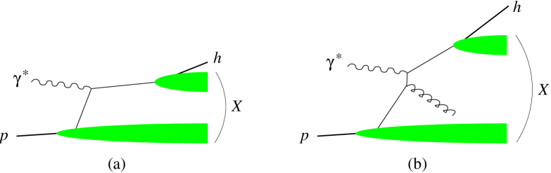
Figure 3: Semi-inclusive hadron production $\gamma^{*}p\to hX$ at large $Q^{2}$. (a) Born level graph. (b) A next-to-leading order graph where the hadron $h$ has transverse momentum of order $Q$.

For definiteness let us express the leading-twist results from [17] in terms of $\gamma^{*}p$ cross sections and interference terms. Using the abbreviation

$$\Gamma=\frac{4\pi^{3}\alpha_{\rm em}}{Q^{2}}\,\frac{x_{B}}{1-x_{B}}$$ (47)

we can write

$$\frac{1}{2}\,\Bigg{[}\frac{d\sigma_{++}^{++}}{dz\,d\mbox{\boldmath{$P$}}_{hT}^{2}}+\frac{d\sigma_{++}^{--}}{dz\,d\mbox{\boldmath{$P$}}_{hT}^{2}}\Bigg{]} = \Gamma\,\mathcal{F}\Big{[}f_{1}D_{1}\Big{]},$$

$$\frac{1}{2}\,\Bigg{[}\frac{d\sigma_{++}^{++}}{dz\,d\mbox{\boldmath{$P$}}_{hT}^{2}}-\frac{d\sigma_{++}^{--}}{dz\,d\mbox{\boldmath{$P$}}_{hT}^{2}}\Bigg{]} = \Gamma\,\mathcal{F}\Big{[}g_{1}D_{1}\Big{]},$$

$$\mathrm{Re}\,\frac{d\sigma_{+-}^{++}}{dz\,d\mbox{\boldmath{$P$}}_{hT}^{2}} = \Gamma\,\mathcal{F}\Bigg{[}\,\frac{|\mbox{\boldmath{$p$}}_{T}|\,|\mbox{\boldmath{$k$}}_{T}|\cos(\varphi_{p}+\varphi_{k})}{M_{p}\,M_{h}}\;h_{1}^{\perp}H_{1}^{\perp}\,\Bigg{]},$$

$$\mathrm{Im}\,\frac{d\sigma_{+-}^{++}}{dz\,d\mbox{\boldmath{$P$}}_{hT}^{2}} = \Gamma\,\mathcal{F}\Bigg{[}\,\frac{|\mbox{\boldmath{$p$}}_{T}|\,|\mbox{\boldmath{$k$}}_{T}|\cos(\varphi_{p}+\varphi_{k})}{M_{p}\,M_{h}}\;h_{1L}^{\perp}H_{1}^{\perp}\,\Bigg{]},$$

$$\mathrm{Re}\,\frac{d\sigma_{++}^{+-}}{dz\,d\mbox{\boldmath{$P$}}_{hT}^{2}} = \Gamma\,\mathcal{F}\Bigg{[}\,\frac{|\mbox{\boldmath{$p$}}_{T}|\cos\varphi_{p}}{M_{p}}\;g_{1T}D_{1}\,\Bigg{]},$$

$$\mathrm{Im}\,\frac{d\sigma_{++}^{+-}}{dz\,d\mbox{\boldmath{$P$}}_{hT}^{2}} = \Gamma\,\mathcal{F}\Bigg{[}\,\frac{|\mbox{\boldmath{$p$}}_{T}|\cos\varphi_{p}}{M_{p}}\;f_{1T}^{\perp}D_{1}^{\phantom{\perp}}\,\Bigg{]},$$

$$\mathrm{Im}\,\frac{d\sigma_{+-}^{+-}}{dz\,d\mbox{\boldmath{$P$}}_{hT}^{2}} = \Gamma\,\mathcal{F}\Bigg{[}\,\frac{|\mbox{\boldmath{$k$}}_{T}|\cos\varphi_{k}}{M_{h}}\;2h_{1}^{\phantom{\perp}\!\!\!}H_{1}^{\perp}\,\Bigg{]},$$

$$\mathrm{Im}\,\frac{d\sigma_{+-}^{-+}}{dz\,d\mbox{\boldmath{$P$}}_{hT}^{2}} = \Gamma\,\mathcal{F}\Bigg{[}\,\frac{|\mbox{\boldmath{$p$}}_{T}|^{2}|\mbox{\boldmath{$k$}}_{T}|\cos(2\varphi_{p}+\varphi_{k})}{M_{p}^{2}\,M_{h}}\;h_{1T}^{\perp}H_{1}^{\perp}\,\Bigg{]},\hskip 40.00006pt$$ (48)

with convolution integrals given by

$$\mathcal{F}\Big{[}wfD\Big{]}=\sum_{a=q,\bar{q}}e_{a}^{2}\,\int d^{2}\mbox{\boldmath{$p$}}_{T}\,d^{2}\mbox{\boldmath{$k$}}_{T}^{\phantom{*}}\,\delta^{(2)}\Big{(}\mbox{\boldmath{$p$}}_{T}^{\phantom{*}}-\mbox{\boldmath{$k$}}_{T}^{\phantom{*}}-\mbox{\boldmath{$P$}}_{hT}^{\phantom{*}}/z\Big{)}\;w(\mbox{\boldmath{$p$}}_{T},\mbox{\boldmath{$k$}}_{T}^{\phantom{*}})\,f^{a}(x_{B},\mbox{\boldmath{$p$}}_{T}^{2})\;D^{a}(z,z^{2}\mbox{\boldmath{$k$}}_{T}^{2}),$$ (49)

where $f$ represents a parton density, $D$ a fragmentation function, and $w$ an additional weight function. To write the weight functions in a compact way we have used angles $\varphi_{p}=\angle(\mbox{\boldmath{$p$}}_{T}^{\phantom{*}},\mbox{\boldmath{$P$}}_{hT}^{\phantom{*}})$ and $\varphi_{k}=\angle(\mbox{\boldmath{$k$}}_{T},\mbox{\boldmath{$P$}}_{hT})$ in the transverse plane. The quark or antiquark densities (in lowercase symbols) depend on $x_{B}$ and on the transverse momentum $\mbox{\boldmath{$p$}}_{T}$ of the parton relative to the proton. The fragmentation functions (in uppercase symbols) depend on $z$ and on the transverse momentum $\mbox{\boldmath{$k$}}_{T}$ of the parton relative to the hadron $h$ (or the transverse momentum $-z\mbox{\boldmath{$k$}}_{T}$ of $h$ relative to the parton). We note that some of the convolutions in (5) acquire an explicit minus sign when the integrals over $\mbox{\boldmath{$p$}}_{T}$ and $\mbox{\boldmath{$k$}}_{T}^{\phantom{*}}$ are carried out, see e.g. App. D in [15]. As remarked in [16], the convolutions (49) factorize into separate transverse momentum integrals over parton densities and over fragmentation functions if one forms weighted cross sections $\int d\mbox{\boldmath{$P$}}_{hT}^{2}\,|\mbox{\boldmath{$P$}}_{hT}^{\phantom{*}}/z\,|^{M}\,d\sigma_{mn}^{ij}/(dz\,d\mbox{\boldmath{$P$}}_{hT}^{2})$ with the power $M=|m-n-i+j|$ we encountered in (32). We shall not discuss all parton densities and fragmentation functions here (see [15, 16] for their definitions and [19] for an overview), but point out two terms of particular interest in ongoing and planned experiments [21, 22, 23, 24]. The Sivers function $f_{1T}^{\perp}$ together with the usual unpolarized fragmentation function $D_{1}$ appears in $\mathrm{Im}\,\sigma_{++}^{+-}$, and the transversity distribution $h_{1}$ comes together with the Collins fragmentation function $H_{1}^{\perp}$ in $\mathrm{Im}\,\sigma_{+-}^{+-}$. Many investigations have shown these functions to reveal subtle aspects of the dynamics and the structure of hadrons, see e.g. [20, 25] for recent reviews.

We notice in (5) that all possible cross sections and interference terms with transverse photons are nonzero. The results of [15, 16, 18] show that all interference terms $\sigma_{+0}^{ij}$ are nonvanishing as well. Taking into account the $Q^{2}$ behavior specified above and keeping in mind that $\sin\theta$ is of order $1/Q$, we can now discuss the relative size of terms which have the same dependence on $\phi$ and $\phi_{S}$ in the cross sections (33) and (34) for definite target polarization with respect to the beam.

1. For longitudinal target polarization the Sivers and Collins terms, $\mathrm{Im}\,\sigma_{++}^{+-}$ and $\mathrm{Im}\,\sigma_{+-}^{+-}$, come with a factor $\sin\theta$ and thus appear with the same power in $1/Q$ as the twist-three interference term $\mathrm{Im}\,(\sigma_{+0}^{++}-\sigma_{+0}^{--})$. For a transversely polarized target, this twist-three term is multiplied with $\sin\theta$ and thus suppressed by $1/Q^{2}$ compared with the Sivers or the Collins term. Furthermore, the Sivers term $\mathrm{Im}\,\sigma_{++}^{+-}$ always comes together with $\mathrm{Im}\,\sigma_{00}^{+-}$, which is $1/Q^{2}$ suppressed according to our above discussion.

2. For the $\phi$ independent terms in the cross section the situation is reverse (and well-known from inclusive DIS). Here it is for transverse target polarization that both the twist-two cross section difference $\sigma_{++}^{++}-\sigma_{++}^{--}$ and the twist-three term $\mathrm{Re}\,\sigma_{+0}^{+-}$ appear with the same power in $1/Q$. For a longitudinally polarized target this twist-three term is accompanied by $\sin\theta$ and thus down by $1/Q^{2}$ compared with $\sigma_{++}^{++}-\sigma_{++}^{--}$.

For the terms with $\cos\phi$ and $\cos(\phi-\phi_{S})$ in the polarized cross sections (33) and (34) the situation is as in case 1, and for the terms with $\sin(2\phi)$ and $\sin(2\phi-\phi_{S})$ as in case 2.

In those cases where a “competing term” in the cross section is suppressed by $1/Q^{2}$, one may argue that it should be consistently neglected in an analysis based on theoretical results with accuracy only up to order $1/Q$. After all, quantities like $\mathrm{Im}\,\sigma_{++}^{+-}$ have themselves $1/Q^{2}$ suppressed contributions in addition to the leading-twist part which one would like to extract. In general, subtracting one particular type of power-suppressed term from an observable can improve the comparison with leading-twist theory, but it can also make it worse, since different power-suppressed terms may have opposite sign and partially compensate each other. Our case is however special. Taking for example the $1/Q^{2}$ suppressed quantities $\varepsilon\mathrm{Im}\,\sigma_{00}^{+-}$ and $\sin\theta\sqrt{\varepsilon(1+\varepsilon)}\,\mathrm{Im}\,(\sigma_{+0}^{++}-\sigma_{+0}^{--})$, which compete with $\mathrm{Im}\,\sigma_{++}^{+-}$ in the $\sin(\phi-\phi_{S})$ term, we see that they come with a different dependence on $\varepsilon$. Since the $\sigma_{mn}^{ij}$ are independent of this variable, these power-suppressed terms can in general not compensate power corrections in $\mathrm{Im}\,\sigma_{++}^{+-}$ itself. This provides some theoretical motivation to try and separate such contributions, which may be of practical relevance especially if a twist-two term is “accidentally” small because the relevant parton distributions or fragmentation functions are.

Let us finally remark on loop corrections to the Born level formulae on which we have based our discussion so far. At leading accuracy in $1/Q$ these have been recently investigated in [27, 28]. Note that at next-to-leading order in $\alpha_{s}$ there are hard-scattering graphs where two partons with transverse momenta of order $Q$ are produced, see Fig. 3b. It was emphasized in [27] that such graphs do not contribute when $\mbox{\boldmath{$P$}}_{hT}$ is small compared with $Q$ and can be generated from the transverse momentum dependence in the parton densities and fragmentation functions, as expressed in (49). They do however contribute if one integrates the cross section over all $\mbox{\boldmath{$P$}}_{hT}$ (or takes $\mbox{\boldmath{$P$}}_{hT}$ weighted cross sections as mentioned above). They produce effects at leading order in $1/Q$ and can be evaluated using standard collinear factorization, with parton densities and fragmentation functions that are integrated over the transverse parton momentum. In particular, these graphs generate an order $\alpha_{s}$ contribution to the longitudinal cross section $\sigma_{00}^{++}$, just as in the well-known case of inclusive DIS. Explicit calculation for an unpolarized target shows that they also generate a $\cos\phi$ and $\cos(2\phi)$ modulation in the cross section [29], described by the interference terms $\mathrm{Re}\,(\sigma_{+0}^{++}+\sigma_{+0}^{--})$ and $\mathrm{Re}\,\sigma_{+-}^{++}$. The lepton polarization dependence for an unpolarized target is due to $\mathrm{Im}\,(\sigma_{+0}^{++}+\sigma_{+0}^{--})$. Because of time reversal invariance, this term requires an absorptive part in the amplitude and thus appears only at order $\alpha_{s}^{2}$ in the large $\mbox{\boldmath{$P$}}_{hT}$ region [30].

6 Exclusive meson production

Exclusive electroproduction of light mesons such as $\ell p\to\ell\rho^{0}p$ or $\ell p\to\ell\pi^{+}n$ provides opportunities to study generalized parton distributions (GPDs), see [4, 31] for recent reviews. In the limit of large $Q^{2}$ at fixed $x_{B}$ and $t$, the $\gamma^{*}p$ amplitude factorizes into the convolution of a hard-scattering subprocess with generalized parton distributions in the nucleon and the light-cone distribution amplitude of the produced meson (see Fig. 4). The factorization theorem shows that the leading transitions in the large $Q^{2}$ limit have both the virtual photon and the produced meson longitudinally polarized, all other transitions being suppressed by at least one power of $1/Q$ [32, 33]. This gives a hierarchy opposite to the one we have encountered for semi-inclusive production in Sect. 5:

1. The only leading-twist observables are the longitudinal cross section $\sigma_{00}^{++}$ and the interference term $\sigma_{00}^{+-}$.

2. Transverse-longitudinal interference terms $\sigma_{+0}^{ij}$ are at least one power of $1/Q$ down compared with $\sigma_{00}^{++}$.

3. Cross sections and interference terms $\sigma_{++}^{ij}$ and $\sigma_{+-}^{ij}$ with transverse photon polarization are suppressed by at least $1/Q^{2}$ compared with $\sigma_{00}^{++}$.

Using the abbreviation

$$\Gamma^{\prime}=\frac{\alpha_{\rm em}}{Q^{6}}\,\frac{x_{B}^{2}}{1-x_{B}}$$ (50)

the leading-twist results given in [4, 31] can written as

$$\frac{1}{\Gamma^{\prime}}\,\frac{d\sigma_{00}^{++}}{dt} = (1-\xi^{2})\,|\mathcal{H}_{M}|^{2}-\left(\xi^{2}+\frac{t}{4M_{p}^{2}}\right)|\mathcal{E}_{M}|^{2}-2\xi^{2}\,\mathrm{Re}\,(\mathcal{E}_{M}^{*}\mathcal{H}_{M}^{\phantom{*}}),$$

$$\frac{1}{\Gamma^{\prime}}\;\mathrm{Im}\,\frac{d\sigma_{00}^{+-}}{dt} = {}-\sqrt{1-\xi^{2}}\,\frac{\sqrt{t_{0}-t}}{M_{p}}\,\mathrm{Im}\,(\mathcal{E}_{M}^{*}\mathcal{H}_{M}^{\phantom{*}})$$ (51)

for mesons with natural parity like $\rho^{0}$, $\rho^{+}$, $f_{2}$, and as

$$\frac{1}{\Gamma^{\prime}}\,\frac{d\sigma_{00}^{++}}{dt} = (1-\xi^{2})\,|\tilde{\mathcal{H}}_{M}|^{2}-\xi^{2}\frac{t}{4M_{p}^{2}}\,|\tilde{\mathcal{E}}_{M}|^{2}-2\xi^{2}\,\mathrm{Re}\,(\tilde{\mathcal{E}}_{M}^{*}\tilde{\mathcal{H}}_{M}^{\phantom{*}}),\hskip 28.00006pt$$

$$\frac{1}{\Gamma^{\prime}}\;\mathrm{Im}\,\frac{d\sigma_{00}^{+-}}{dt} = \sqrt{1-\xi^{2}}\,\frac{\sqrt{t_{0}-t}}{M_{p}}\,\xi\,\mathrm{Im}\,(\tilde{\mathcal{E}}_{M}^{*}\tilde{\mathcal{H}}_{M}^{\phantom{*}})$$ (52)

for mesons with unnatural parity like $\pi^{0}$, $\pi^{+}$, $\eta$. In the kinematical factors on the right-hand side we have used the scaling variable $\xi$ and the smallest kinematically allowed momentum transfer $-t_{0}$, given by

$$\xi=\frac{x_{B}}{2-x_{B}},\qquad\qquad\qquad-t_{0}=\frac{4\xi^{2}M_{p}^{2}}{1-\xi^{2}}$$ (53)

up to relative corrections of order $x_{B}M_{p}^{2}/Q^{2}$, $x_{B}\,t/Q^{2}$ and $M_{h}^{2}/Q^{2}$. Note that $\sqrt{t_{0}-t}\propto|\mbox{\boldmath{$P$}}_{hT}|$, so that the behavior of $\mathrm{Im}\,d\sigma_{00}^{+-}/dt$ illustrates our general result (32).

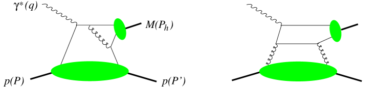
Figure 4: Example graphs for exclusive production of a meson $M$ at large $Q^{2}$. Instead of the proton there may be a different baryon in the final state. The lower blobs represent twist-two generalized parton distributions, and the upper blobs stand for the twist-two distribution amplitude of the meson.

The quantities $\mathcal{H}_{M}$, $\mathcal{E}_{M}$, $\tilde{\mathcal{H}}_{M}$, $\tilde{\mathcal{E}}_{M}$ are integrals over the GPDs $H$, $E$, $\tilde{H}$, $\tilde{E}$ appropriate for the production of the meson $M$ (given in App. C for $\ell p\to\ell\rho^{0}p$ and $\ell p\to\ell\pi^{+}n$). They depend on $\xi$, $t$ and $Q^{2}$, where the dependence on $Q^{2}$ is only logarithmic and reflects the familiar scaling violations from loop corrections to the hard-scattering kernels. We note that for mesons with natural parity both quark and gluon GPDs in general contribute at leading order in $\alpha_{s}$, whereas for mesons with unnatural parity only quark distributions appear at this accuracy [31].

The interest of measuring $\mathrm{Im}\,d\sigma_{00}^{+-}/dt$ in addition to $d\sigma_{00}^{++}/dt$ is immediately clear from (6) and (6). The combination of these two observables provides a handle to separate the contributions from the GPDs $H$ and $E$ or $\tilde{H}$ and $\tilde{E}$, which describe different spin dependence. The nucleon helicity-flip distributions $E^{q}$ and $E^{g}$ are of particular interest because they carry information about the contribution from the orbital angular momentum of quarks and gluons to the total spin of the proton [5]. With the $Q^{2}$ behavior discussed above, we find from (34) that with transverse target polarization one can obtain $\mathrm{Im}\,\sigma_{00}^{+-}$ from the $\sin(\phi-\phi_{S})$ dependent term of the $\ell p$ cross section, where it comes together with the terms $\mathrm{Im}\,\sigma_{++}^{+-}$ and $\sin\theta\,\mathrm{Im}\,(\sigma_{+0}^{++}-\sigma_{+0}^{--})$, both of which are suppressed by at least $1/Q^{2}$. In the cross section (33) for longitudinal target polarization, $\sin\theta\,\mathrm{Im}\,\sigma_{00}^{+-}$ and $\mathrm{Im}\,(\sigma_{+0}^{++}-\sigma_{+0}^{--})$ contribute to the $\sin\phi$ dependence with the same power of $1/Q$, together with at least $1/Q^{2}$ suppressed terms $\sin\theta\,\mathrm{Im}\,\sigma_{++}^{+-}$ and $\sin\theta\,\mathrm{Im}\,\sigma_{+-}^{+-}$. We note that a nonzero effect for this $\sin\phi$ modulation has been measured in $ep\to e\pi^{+}n$ by HERMES [35].

As discussed in the previous section, one may want to extract separate $\gamma^{*}p$ cross sections and interference terms without an a priori assumption on their relative size. The leading-twist interference term $\mathrm{Im}\,\sigma_{00}^{+-}$ in (6) could for instance be “accidentally” small because $\mathcal{E}_{M}$ is much smaller than $\mathcal{H}_{M}$ or because their relative phase is close to zero. Combining data for transverse and longitudinal target polarization one can separate the terms $\mathrm{Im}\,(\sigma_{++}^{+-}+\varepsilon\sigma_{00}^{+-})$, $\mathrm{Im}\,\sigma_{+-}^{+-}$ and $\mathrm{Im}\,(\sigma_{+0}^{++}-\sigma_{+0}^{--})$, provided that one measures both the $\sin(\phi-\phi_{S})$ and $\sin(\phi+\phi_{S})$ dependence for a transversely polarized target. Without the Rosenbluth technique one can however not isolate the longitudinal contribution in $\mathrm{Im}\,(\sigma_{++}^{+-}+\varepsilon\sigma_{00}^{+-})$, nor the longitudinal part from $\sigma_{T}+\varepsilon\sigma_{L}$ in the unpolarized cross section.

For electroproduction of vector mesons one experimentally finds that the ratio $\sigma_{L}/\sigma_{T}$ is not very large for $Q^{2}$ of a few GeV² [10, 36], which means that the predicted power suppression of transverse photon amplitudes is numerically not yet very effective in this kinematics. In addition one finds that transitions with the same helicity for photon and meson are clearly larger than those changing the helicity [10, 36], which is commonly referred to as approximate $s$-channel helicity conservation. The largest power suppressed amplitudes are hence those from a transverse photon to a transverse vector meson. A possibility to remove this particularly important type of power correction in an analysis is to measure the decay angular distribution of the vector meson, say in $\rho\to\pi^{+}\pi^{-}$. Here we can make use of our result in Sect. 4. If only the dependence on the polar decay angle $\vartheta$ but not the azimuth $\varphi$ is considered, our cross section formulae (33) and (34) can be made differential in $\cos\vartheta$. Different helicities of the $\rho$ do not interfere if $\varphi$ is integrated over, so that for all $m,n$ and $i,j$ we have

$$\frac{d\sigma_{mn}^{ij}(\gamma^{*}p\to\pi^{+}\pi^{-}p)}{d(\cos\vartheta)}=\frac{3\cos^{2}\!\vartheta}{2}\,\sigma_{mn}^{ij}(\gamma^{*}p\to\rho_{L}\hskip 1.0ptp)+\frac{3\sin^{2}\!\vartheta}{4}\,\sigma_{mn}^{ij}(\gamma^{*}p\to\rho_{T}\hskip 1.0ptp)$$ (54)

with $\gamma^{*}p$ cross sections and interference terms for longitudinal and transverse $\rho$ polarization. Since $\sigma_{++}^{ij}(\rho_{L})$ is the product of two $s$-channel helicity nonconserving amplitudes, it should be negligible in $\sigma_{++}^{ij}(\rho_{L})+\varepsilon\sigma_{00}^{ij}(\rho_{L})$, unless $\varepsilon$ is small. Using the $\vartheta$ dependence in (54) to project out the $\rho_{L}$ contribution from the $\sin(\phi-\phi_{S})$ term in the cross section will hence help toward isolating the twist-two observable $\sigma_{00}^{+-}(\rho_{L})$.

We finally mention that an angular analysis analogous to (54) can also be performed for the production of continuum $\pi^{+}\pi^{-}$ pairs, where one can measure the interference between partial waves with different total spin of the pion pair, see [37, 31] and [38]. The $\vartheta$ dependence for interference terms $d\sigma_{mn}^{+-}/(d\cos\vartheta)$ is the same as for the terms $d\sigma_{mn}^{++}/(d\cos\vartheta)$ accessible with an unpolarized target.

7 Positivity constraints

In Sect. 3 we introduced $\gamma^{*}p$ cross sections and interference terms for specific polarization states. The $\gamma^{*}p$ cross section must be positive or zero for any polarization state of the photon-proton system, so that $\sum_{ijmn}(c_{m}^{i})^{*}\,\sigma_{mn}^{ij}\,c_{n}^{\hskip 1.0ptj}\geq 0$ for arbitrary complex coefficients $c_{m}^{i}$. This means that the matrix

$$M=\left(\begin{array}[]{cccccc}\sigma_{00}^{++}&i\,\mathrm{Im}\,\sigma_{00}^{+-}&(\sigma_{+0}^{++})^{*}&(\sigma_{+0}^{-+})^{*}&-(\sigma_{+0}^{--})^{*}&(\sigma_{+0}^{+-})^{*}\\ -i\,\mathrm{Im}\,\sigma_{00}^{+-}&\sigma_{00}^{++}&(\sigma_{+0}^{+-})^{*}&(\sigma_{+0}^{--})^{*}&(\sigma_{+0}^{-+})^{*}&-(\sigma_{+0}^{++})^{*}\\ \sigma_{+0}^{++}&\sigma_{+0}^{+-}&\sigma_{++}^{++}&\sigma_{++}^{+-}&\sigma_{+-}^{++}&i\,\mathrm{Im}\,\sigma_{+-}^{+-}\\ \sigma_{+0}^{-+}&\sigma_{+0}^{--}&(\sigma_{++}^{+-})^{*}&\sigma_{++}^{--}&i\,\mathrm{Im}\,\sigma_{+-}^{-+}&(\sigma_{+-}^{++})^{*}\\ -\sigma_{+0}^{--}&\sigma_{+0}^{-+}&(\sigma_{+-}^{++})^{*}&-i\,\mathrm{Im}\,\sigma_{+-}^{-+}&\sigma_{++}^{--}&-(\sigma_{++}^{+-})^{*}\\ \sigma_{+0}^{+-}&-\sigma_{+0}^{++}&-i\,\mathrm{Im}\,\sigma_{+-}^{+-}&\sigma_{+-}^{++}&-\sigma_{++}^{+-}&\sigma_{++}^{++}\end{array}\right)$$ (55)

formed by $M_{(mi)(nj)}=\sigma_{mn}^{ij}$ must be positive semidefinite, where the rows and columns are ordered such that they correspond to the combinations $(0,+\frac{1}{2}),(0,-\frac{1}{2}),(+1,+\frac{1}{2}),(+1,-\frac{1}{2}),(-1,+\frac{1}{2}),(-1,-\frac{1}{2})$ of photon and proton helicities. In writing down (55) we have used the relations (28) from hermiticity and parity invariance. We have not been able to find closed expressions for the eigenvalues of this matrix (and if they existed, they might be too complicated to be useful in practice). More tractable sets of positivity bounds can be obtained if one uses that submatrices of $M$ are also positive semidefinite. As simple example is the submatrix for longitudinal photons, formed from the first and second rows and columns of $M$, whose positivity implies

$$|\,\mathrm{Im}\,\sigma_{00}^{+-}|\leq\sigma_{00}^{++}.$$ (56)

The submatrix for transverse photons, formed by the third to sixth rows and columns of $M$, has eigenvalues

$$2e_{1,2}=\sigma_{++}^{++}-\mathrm{Im}\,\sigma_{+-}^{+-}+\sigma_{++}^{--}+\mathrm{Im}\,\sigma_{+-}^{-+}$$

$${}\pm\sqrt{(\sigma_{++}^{++}-\mathrm{Im}\,\sigma_{+-}^{+-}-\sigma_{++}^{--}-\mathrm{Im}\,\sigma_{+-}^{-+})^{2}+4(\mathrm{Re}\,\sigma_{+-}^{++}-\mathrm{Im}\,\sigma_{++}^{+-})^{2}+4(\mathrm{Re}\,\sigma_{++}^{+-}+\mathrm{Im}\,\sigma_{+-}^{++})^{2}}\;,$$

$$2e_{3,4}=\sigma_{++}^{++}+\mathrm{Im}\,\sigma_{+-}^{+-}+\sigma_{++}^{--}-\mathrm{Im}\,\sigma_{+-}^{-+}$$ (57)

$${}\pm\sqrt{(\sigma_{++}^{++}+\mathrm{Im}\,\sigma_{+-}^{+-}-\sigma_{++}^{--}+\mathrm{Im}\,\sigma_{+-}^{-+})^{2}+4(\mathrm{Re}\,\sigma_{+-}^{++}+\mathrm{Im}\,\sigma_{++}^{+-})^{2}+4(\mathrm{Re}\,\sigma_{++}^{+-}-\mathrm{Im}\,\sigma_{+-}^{++})^{2}}\;.\hskip 30.00005pt$$

Note that $e_{3}$ and $e_{4}$ are obtained from $e_{1}$ and $e_{2}$ by changing the signs of all proton helicity-flip terms $\sigma_{mn}^{+-}$. All four eigenvalues (7) must be nonnegative, which implies

$$|\,\mathrm{Im}\,\sigma_{+-}^{+-}|\leq\sigma_{++}^{++},\qquad\qquad|\,\mathrm{Im}\,\sigma_{+-}^{-+}|\leq\sigma_{++}^{--},$$ (58)

and

$$\Big{(}\mathrm{Re}\,\sigma_{+-}^{++}-\mathrm{Im}\,\sigma_{++}^{+-}\Big{)}^{2}+\Big{(}\mathrm{Re}\,\sigma_{++}^{+-}+\mathrm{Im}\,\sigma_{+-}^{++}\Big{)}^{2} \leq \Big{(}\sigma_{++}^{++}-\mathrm{Im}\,\sigma_{+-}^{+-}\Big{)}\,\Big{(}\sigma_{++}^{--}+\mathrm{Im}\,\sigma_{+-}^{-+}\Big{)},$$

$$\Big{(}\mathrm{Re}\,\sigma_{+-}^{++}+\mathrm{Im}\,\sigma_{++}^{+-}\Big{)}^{2}+\Big{(}\mathrm{Re}\,\sigma_{++}^{+-}-\mathrm{Im}\,\sigma_{+-}^{++}\Big{)}^{2} \leq \Big{(}\sigma_{++}^{++}+\mathrm{Im}\,\sigma_{+-}^{+-}\Big{)}\,\Big{(}\sigma_{++}^{--}-\mathrm{Im}\,\sigma_{+-}^{-+}\Big{)}.$$ (59)

One can easily obtain inequalities that are weaker than (7) but involve fewer interference terms, e.g. by omitting one of the squared terms on the left-hand-sides. Adding the bounds (7) one has

$$(\mathrm{Re}\,\sigma_{+-}^{++})^{2}+(\mathrm{Im}\,\sigma_{++}^{+-})^{2}+(\mathrm{Re}\,\sigma_{++}^{+-})^{2}+(\mathrm{Im}\,\sigma_{+-}^{++})^{2}\leq(\sigma_{++}^{++})\,(\sigma_{++}^{--})-(\mathrm{Im}\,\sigma_{+-}^{+-})\,(\mathrm{Im}\,\sigma_{+-}^{-+}),$$ (60)

where any of the terms on the left-hand side can be omitted. We note that the submatrix of $M$ formed by the 1st, 2nd, 4th and 5th rows and columns has eigenvalues given in analytic form similar to (7), as well as the submatrix formed by the 1st, 2nd, 3rd and 6th rows and columns. This provides inequalities similar to (7) which involve different cross sections and interference terms.

As already mentioned, the dependence of the polarized $\ell p$ cross section on $\phi$ and $\phi_{S}$ allows one to separate all $\gamma^{*}p$ cross sections and interference terms, except for

$$\sigma_{\varepsilon}^{++}={\textstyle\frac{1}{2}}(\sigma_{++}^{++}+\sigma_{++}^{--})+\varepsilon\sigma_{00}^{++}=\sigma_{T}+\varepsilon\sigma_{L},\qquad\qquad\mathrm{Im}\,\sigma_{\varepsilon}^{+-}=\mathrm{Im}\,(\sigma_{++}^{+-}+\varepsilon\sigma_{00}^{+-}),$$ (61)

whose individual contributions from transverse and longitudinal photons can only be disentangled by the Rosenbluth technique. Let us show how the bounds (7) restrict the longitudinal contributions $\varepsilon\sigma_{L}$ and $\varepsilon\,\mathrm{Im}\,\sigma_{00}^{+-}$ to the measurable combinations $\sigma_{\varepsilon}^{++}$ and $\mathrm{Im}\,\sigma_{\varepsilon}^{+-}$. For simplicity we start from the bound (60) and omit the term $\mathrm{Re}\,\sigma_{++}^{+-}$, whose extraction requires measurement of the angular dependence in a double spin asymmetry. We then have

$$(A-\varepsilon\sigma_{L})\,(B-\varepsilon\sigma_{L})-(C-\varepsilon\,\mathrm{Im}\,\sigma_{00}^{+-})^{2}\geq D,\qquad\qquad\varepsilon\sigma_{L}\leq{\textstyle\frac{1}{2}}(A+B),$$ (62)

where

$$A = \sigma_{\varepsilon}^{++}+{\textstyle\frac{1}{2}}(\sigma_{++}^{++}-\sigma_{++}^{--}),\qquad\quad B=\sigma_{\varepsilon}^{++}-{\textstyle\frac{1}{2}}(\sigma_{++}^{++}-\sigma_{++}^{--}),\qquad\quad C=\mathrm{Im}\,\sigma_{\varepsilon}^{+-},$$

$$D = (\mathrm{Re}\,\sigma_{+-}^{++})^{2}+(\mathrm{Im}\,\sigma_{+-}^{++})^{2}+(\mathrm{Im}\,\sigma_{+-}^{+-})\,(\mathrm{Im}\,\sigma_{+-}^{-+})$$ (63)

are measurable without Rosenbluth separation. The corresponding allowed region in the plane of $\sigma_{L}$ and $\mathrm{Im}\,\sigma_{00}^{+-}$ is bounded on the right by a branch of the hyperbola defined by $(A-\varepsilon\sigma_{L})\,(B-\varepsilon\sigma_{L})-(C-\varepsilon\,\mathrm{Im}\,\sigma_{00}^{+-})^{2}=D$. Together with $|\mathrm{Im}\,\sigma_{00}^{+-}|\leq\sigma_{L}$ this leaves the shaded region shown in Fig. 5. Note that this region depends on $\varepsilon$, both explicitly through the factors multiplying $\sigma_{L}$ and $\mathrm{Im}\,\sigma_{00}^{+-}$ in (62) and implicitly through $\sigma_{\varepsilon}^{++}$ and $\mathrm{Im}\,\sigma_{\varepsilon}^{+-}$ in $A$, $B$ and $C$. Stronger restrictions on $\sigma_{L}$ and $\mathrm{Im}\,\sigma_{00}^{+-}$ are obtained in the same manner if one starts with the two bounds (7), each of which can be written in the form (62) with suitable coefficients $A$, $B$, $C$, $D$.

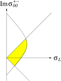
Figure 5: Region in the plane of $\sigma_{L}$ and $\mathrm{Im}\,\sigma_{00}^{+-}$ allowed by the positivity bounds (56) and (62).

8 Deeply virtual Compton scattering

In this section we discuss the specific case of DVCS, which is measured in the exclusive electroproduction process

$$\ell(l)+p(P)\to\ell(l^{\prime})+\gamma(q^{\prime})+p(P^{\prime}),$$ (64)

where a real photon with momentum $q^{\prime}$ now plays the role taken in the previous sections by the produced hadron $h$ with momentum $P_{h}$. We use the same kinematical variables as before, introduced in Sect. 2 and in (25) and (53). In particular, the azimuthal angle $\phi$ is defined as in Fig. 1 with $P_{h}$ replaced by $q^{\prime}$.

DVCS is one of the most valuable sources of information about generalized parton distributions. One reason is that in the reaction (64) Compton scattering interferes with the Bethe-Heitler process, see Fig. 6. The $\ell p$ cross section thus receives contributions

$$d\sigma(\ell p\to\ell\gamma p)=d\sigma_{\it VCS}+d\sigma_{\it BH}+d\sigma_{\it INT}$$ (65)

from Compton scattering and from the Bethe-Heitler process, as well as from their interference term. The Compton part $d\sigma_{\it VCS}$ of the cross section has the same general structure as discussed in Sect. 3. With suitable kinematics and observables, one can however also access the interference term $d\sigma_{\it INT}$, which has a simple linear dependence on the helicity amplitudes of the subprocess $\gamma^{*}p\to\gamma p$ (as opposed to a quadratic dependence in $d\sigma_{\it VCS}$). In addition, the interference term provides access to the phases of these subprocess amplitudes.

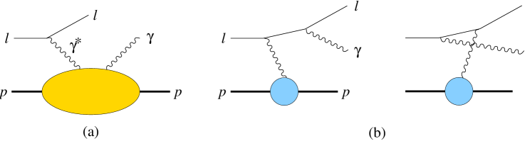
Figure 6: Graphs for virtual Compton scattering (a) and for the Bethe-Heitler process (b).

In the generalized Bjorken limit of large $Q^{2}$ at fixed $x_{B}$ and $t$, the Compton amplitude can be written as the convolution of hard-scattering kernels with GPDs [39]. The detailed dependence of the $\ell p$ cross section on these convolutions has been given in [40] at the leading and first subleading order in $1/Q$. To see which combinations of GPDs are measurable with which polarization, we give here the expression of the interference term at leading order in $1/Q$,

$$\frac{d\sigma_{\it INT}}{dx_{B}\,dQ^{2}\,dt\,d\phi\,d\psi} \approx {}-e_{\ell}\,\frac{\alpha_{\mathrm{em}}^{3}}{2\pi^{2}}\,\frac{y^{2}}{Q^{4}}\,\frac{2-x_{B}}{|t|}\,\frac{M_{p}}{Q}\,\sqrt{\frac{2}{\varepsilon(1-\varepsilon)}}\;\frac{1}{P(\cos\phi)}$$ (66)

$$\times\Big{(}\cos\phi\,\mathrm{Re}\,\widehat{M}_{++}+P_{\ell}\sqrt{1-\varepsilon^{2}}\,\sin\phi\,\mathrm{Im}\,\widehat{M}_{++}\phantom{\Big{[}\Big{]}}$$

$${}+S_{L}\Big{[}\sin\phi\,\mathrm{Im}\,\widehat{M}^{\,L}_{++}+P_{\ell}\sqrt{1-\varepsilon^{2}}\,\cos\phi\,\mathrm{Re}\,\widehat{M}^{\,L}_{++}\Big{]}$$

$${}+S_{T}\cos(\phi-\phi_{S})\,\Big{[}\sin\phi\,\mathrm{Im}\,\widehat{M}^{\,S}_{++}+P_{\ell}\sqrt{1-\varepsilon^{2}}\,\cos\phi\,\mathrm{Re}\,\widehat{M}^{\,S}_{++}\Big{]}$$

$${}+S_{T}\sin(\phi-\phi_{S})\;\Big{[}\cos\phi\,\mathrm{Im}\,\widehat{M}^{\,N}_{++}-P_{\ell}\sqrt{1-\varepsilon^{2}}\,\sin\phi\,\mathrm{Re}\,\widehat{M}^{\,N}_{++}\Big{]}\,\Big{)}\,,\hskip 20.00003pt$$

where $e_{\ell}=\pm 1$ is the charge of the lepton beam. Notice that the factor

$$P(\cos\phi)=1-2\cos\phi\,\sqrt{\frac{2(1+\varepsilon)}{\varepsilon}\,\frac{1-\xi}{1+\xi}\,\frac{t_{0}-t}{Q^{2}}}\,+O\Big{(}\frac{1}{Q^{2}}\Big{)}$$ (67)

from the lepton propagators in the Bethe-Heitler amplitude influences the $\phi$ dependence of the cross section. This effect is formally of order $1/Q$ but can be rather important in experimentally relevant kinematics, also because $P(\cos\phi)$ appears in the denominator of (66). The coefficients appearing in (66) are linear combinations of $\gamma^{*}p\to\gamma p$ helicity amplitudes with both photons having helicity $+1$. They can be written in terms of Compton form factors as

$$\widehat{M}_{++} = \sqrt{1-\xi^{2}}\,\frac{\sqrt{t_{0}-t}}{2M_{p}}\,\Bigg{[}F_{1}\mathcal{H}+\xi(F_{1}+F_{2})\tilde{\mathcal{H}}-\frac{t}{4M_{p}^{2}}\,F_{2}\,\mathcal{E}\Bigg{]},$$ (68)

$$\widehat{M}_{++}^{\,L} = \sqrt{1-\xi^{2}}\,\frac{\sqrt{t_{0}-t}}{2M_{p}}\,\Bigg{[}F_{1}\tilde{\mathcal{H}}+\xi(F_{1}+F_{2})\Big{(}{\mathcal{H}}+\frac{\xi}{1+\xi}\,\mathcal{E}\Big{)}-\Big{(}\frac{\xi}{1+\xi}\,F_{1}+\frac{t}{4M_{p}^{2}}\,F_{2}\Big{)}\,\xi\tilde{\mathcal{E}}\Bigg{]},$$

$$\widehat{M}^{\,S}_{++} = \Bigg{[}\xi^{2}\Big{(}F_{1}+\frac{t}{4M_{p}^{2}}\,F_{2}\Big{)}-\frac{t}{4M_{p}^{2}}\,F_{2}\Bigg{]}\tilde{\mathcal{H}}-\Big{(}\frac{t}{4M_{p}^{2}}+\frac{\xi^{2}}{1+\xi}\Big{)}\,\xi(F_{1}+F_{2})\,\mathcal{E}$$

$${}+\Bigg{[}\Big{(}\frac{t}{4M_{p}^{2}}+\frac{\xi^{2}}{1+\xi}\Big{)}\,F_{1}+\frac{t}{4M_{p}^{2}}\,\xi F_{2}\Bigg{]}\,\xi\tilde{\mathcal{E}}-\xi^{2}(F_{1}+F_{2})\mathcal{H}\,,$$

$$\widehat{M}^{\,N}_{++} = {}-\frac{t}{4M_{p}^{2}}\,\Big{(}F_{2}\mathcal{H}-F_{1}\,\mathcal{E}\Big{)}+\xi^{2}\Big{(}F_{1}+\frac{t}{4M_{p}^{2}}\,F_{2}\Big{)}\,(\mathcal{H}+\mathcal{E})-\xi^{2}(F_{1}+F_{2})\Big{(}\tilde{\mathcal{H}}+\frac{t}{4M_{p}^{2}}\,\tilde{\mathcal{E}}\Big{)},$$

with the Dirac and Pauli form factors $F_{1}$ and $F_{2}$ of the proton evaluated at momentum transfer $t$. The term with superscript $S$ (“sideways”) contributes most strongly to the cross section for transverse target polarization in the hadron plane, and the term with superscript $N$ (“normal”) contributes most for target polarization perpendicular to the hadron plane, according to the respective factors $\cos(\phi-\phi_{S})$ and $\sin(\phi-\phi_{S})$ in (66). The Compton form factors are given as integrals over GPDs and read

$$\mathcal{H}(\xi,t) = \sum_{q}e_{q}^{2}\int_{-1}^{1}dx\,H^{q}(x,\xi,t)\,\left(\frac{1}{\xi-x-i\varepsilon}-\frac{1}{\xi+x-i\varepsilon}\right)+O(\alpha_{s}),$$

$$\tilde{\mathcal{H}}(\xi,t) = \sum_{q}e_{q}^{2}\int_{-1}^{1}dx\,\tilde{H}^{q}(x,\xi,t)\,\left(\frac{1}{\xi-x-i\varepsilon}+\frac{1}{\xi+x-i\varepsilon}\right)+O(\alpha_{s}),$$ (69)

where the sums are over quark flavors $q$ with $e_{u}=\frac{2}{3}$ and $e_{d}=e_{s}=-\frac{1}{3}$. The expressions for $\mathcal{E}$ and $\smash{\tilde{\mathcal{E}}}$ are analogous to those of $\mathcal{H}$ and $\smash{\tilde{\mathcal{H}}}$, respectively. In (8) we have suppressed the dependence of the Compton form factors on $Q^{2}$, which arises at order $\alpha_{s}$ in analogy to the scaling violation in deep inelastic structure functions.

We see in (66) that single beam or target spin asymmetries project out the imaginary parts of the Compton form factors, which according to (8) are just GPDs at $x=\pm\xi$ to leading order in $\alpha_{s}$. The real part of $\widehat{M}_{++}$ appears in the unpolarized $\ell p$ cross section, and the real parts of the other three combinations in double spin asymmetries. From (68) one readily finds that separation of all four Compton form factors is possible.

Since $\xi$ is small in a wide range of experimentally relevant kinematics, it is instructive to write

$$\widehat{M}^{\,S}_{++} = -\frac{t}{4M_{p}^{2}}\,\Big{[}F_{2}\tilde{\mathcal{H}}-F_{1}\,\xi\tilde{\mathcal{E}}\,\Big{]}-\xi\frac{t}{4M_{p}^{2}}\,\Big{[}(F_{1}+F_{2})\mathcal{E}-F_{2}\,\xi\tilde{\mathcal{E}}\,\Big{]}+\xi^{2}\,O(\mathcal{H},\mathcal{E},\tilde{\mathcal{H}},\xi\tilde{\mathcal{E}})\,,$$

$$\widehat{M}^{\,N}_{++} = -\frac{t}{4M_{p}^{2}}\,\Big{[}F_{2}\mathcal{H}-F_{1}\mathcal{E}\Big{]}-\xi\frac{t}{4M_{p}^{2}}\,(F_{1}+F_{2})\,\xi\tilde{\mathcal{E}}+\xi^{2}\,O(\mathcal{H},\mathcal{E},\tilde{\mathcal{H}})\,.$$ (70)

For counting powers of $\xi$ we use $\xi\tilde{\mathcal{E}}$ rather than $\tilde{\mathcal{E}}$ in comparison with $\mathcal{H}$, because the contribution to $\tilde{E}$ from pion exchange scales like $\xi^{-1}$, see [4, 31]. The only combination in (68) where the helicity-flip distribution $E$ is not kinematically suppressed compared with other GPDs turns out to be $\widehat{M}^{\,N}_{++}$, which comes with an angular dependence like $\sin(\phi-\phi_{S})\cos\phi$ or $\sin(\phi-\phi_{S})\sin\phi$ in the interference term. Note that one may rewrite

$$\phantom{+}\cos(\phi-\phi_{S})\,\Big{[}\sin\phi\,\mathrm{Im}\,\widehat{M}^{\,S}_{++}+P_{\ell}\sqrt{1-\varepsilon^{2}}\,\cos\phi\,\mathrm{Re}\,\widehat{M}^{\,S}_{++}\Big{]}$$

$$+\sin(\phi-\phi_{S})\;\Big{[}\cos\phi\,\mathrm{Im}\,\widehat{M}^{\,N}_{++}-P_{\ell}\sqrt{1-\varepsilon^{2}}\,\sin\phi\,\mathrm{Re}\,\widehat{M}^{\,N}_{++}\Big{]}$$ (71)

$$= \frac{1}{2}\Big{[}\sin(2\phi-\phi_{S})\,\mathrm{Im}\,(\widehat{M}^{\,S}_{++}+\widehat{M}^{\,N}_{++})+P_{\ell}\sqrt{1-\varepsilon^{2}}\,\cos(2\phi-\phi_{S})\,\mathrm{Re}\,(\widehat{M}^{\,S}_{++}+\widehat{M}^{\,N}_{++})$$

$$\hskip 30.70012pt{}+\sin\phi_{S}\,\mathrm{Im}\,(\widehat{M}^{\,S}_{++}-\widehat{M}^{\,N}_{++})+P_{\ell}\sqrt{1-\varepsilon^{2}}\,\cos\phi_{S}\,\mathrm{Re}\,(\widehat{M}^{\,S}_{++}-\widehat{M}^{\,N}_{++})\,\Big{]}\,,$$

which results in a simpler form of the angular dependence, as we have used in Sect. 3. In terms of dominant contributions from the different GPDs, the combinations $\widehat{M}^{\,S}_{++}$ and $\widehat{M}^{\,N}_{++}$ appear however more natural than their difference and sum, see (8).

Let us now take a closer look at how the different Compton form factors can be extracted from the polarized $\ell p$ cross section. To this end we need the general dependence on the angles $\phi$ and $\phi_{S}$, which has the form [40]

$$\frac{Q^{4}}{y^{2}}\,\frac{d\sigma_{\it BH}}{dx_{B}\,dQ^{2}\,dt\,d\phi\,d\psi} = \frac{1}{|t|}\,\frac{1}{\varepsilon}\,\frac{1}{P(\cos\phi)}\Bigg{(}\sum_{n=0}^{2}\cos(n\phi)\,c_{nU}^{\it BH}+S_{L}P_{\ell}\,\sum_{n=0}^{1}\cos(n\phi)\,c_{nL}^{\it BH}$$

$${}+S_{T}P_{\ell}\,\Big{[}\cos(\phi-\phi_{S})\sum_{n=0}^{1}\cos(n\phi)\,c_{nS}^{\it BH}+\sin(\phi-\phi_{S})\sin\phi\;s_{1N}^{\it BH}\,\Big{]}\Bigg{)},$$

$$\frac{Q^{4}}{y^{2}}\,\frac{d\sigma_{\it VCS}}{dx_{B}\,dQ^{2}\,dt\,d\phi\,d\psi} = \frac{1}{Q^{2}}\,\frac{1}{1-\varepsilon}\Bigg{(}\sum_{n=0}^{2}\cos(n\phi)\,c_{nU}^{\it VCS}+P_{\ell}\sin\phi\;s_{1U}^{\it VCS}$$

$${}+S_{L}\,\sum_{n=1}^{2}\sin(n\phi)\,s_{nL}^{\it VCS}+S_{L}P_{\ell}\,\sum_{n=0}^{1}\cos(n\phi)\,c_{nL}^{\it VCS}$$

$${}+S_{T}\,\Big{[}\sin(\phi-\phi_{S})\sum_{n=0}^{2}\cos(n\phi)\,c_{nN}^{\it VCS}+\cos(\phi-\phi_{S})\sum_{n=1}^{2}\sin(n\phi)\,s_{nS}^{\it VCS}\,\Big{]}$$

$${}+S_{T}P_{\ell}\,\Big{[}\cos(\phi-\phi_{S})\sum_{n=0}^{1}\cos(n\phi)\,c_{nS}^{\it VCS}+\sin(\phi-\phi_{S})\sin\phi\;s_{1N}^{\it VCS}\,\Big{]}\Bigg{)},$$

$$\frac{Q^{4}}{y^{2}}\,\frac{d\sigma_{\it INT}}{dx_{B}\,dQ^{2}\,dt\,d\phi\,d\psi} = {}-e_{\ell}\,\frac{1}{|t|}\,\frac{M_{p}}{Q}\,\frac{1}{\varepsilon\sqrt{1-\varepsilon}}\,\frac{1}{P(\cos\phi)}\Bigg{(}\sum_{n=0}^{3}\cos(n\phi)\,c_{nU}^{\it INT}+P_{\ell}\sum_{n=1}^{2}\sin(n\phi)\,s_{nU}^{\it INT}$$

$${}+S_{L}\sum_{n=1}^{3}\sin(n\phi)\,s_{nL}^{\it INT}+S_{L}P_{\ell}\sum_{n=0}^{2}\cos(n\phi)\,c_{nL}^{\it INT}$$

$${}+S_{T}\Big{[}\sin(\phi-\phi_{S})\sum_{n=0}^{3}\cos(n\phi)\,c_{nN}^{\it INT}+\cos(\phi-\phi_{S})\sum_{n=1}^{3}\sin(n\phi)\,s_{nS}^{\it INT}\,\Big{]}$$

$${}+S_{T}P_{\ell}\Big{[}\cos(\phi-\phi_{S})\sum_{n=0}^{2}\cos(n\phi)\,c_{nS}^{\it INT}+\sin(\phi-\phi_{S})\sum_{n=1}^{2}\sin(n\phi)\,s_{nN}^{\it INT}\,\Big{]}\Bigg{)},$$

where the subscripts $U$, $L$, $S$, $N$ of the angular coefficients $c$ and $s$ indicate an unpolarized target, or longitudinal, sideways or normal target polarization as explained after (68). These angular coefficients depend on $\varepsilon$, $x_{B}$, $Q^{2}$, $t$, and the kinematic prefactors have been chosen such that (up to logarithms in $Q^{2}$) they all remain finite or vanish in the limit of large $Q^{2}$ relevant for the extraction of GPDs. For $\varepsilon\to 0$ the coefficients behave like $c_{n},s_{n}\sim\sqrt{\varepsilon}^{\,n}$, and for $\varepsilon\to 1$ the coefficients accompanied by the lepton polarization $P_{\ell}$ vanish like $\sqrt{1-\varepsilon}$ whereas the others remain finite. We see in (8) that generically $\sigma_{\it BH}$ dominates over $\sigma_{\it VCS}$ in generalized Bjorken kinematics (where $|t|\ll Q^{2}$) except if $\varepsilon$ is sufficiently close to 1. The interference term lies in between $\sigma_{\it BH}$ and $\sigma_{\it VCS}$, and it can most directly be isolated from the difference of cross sections for positive and negative lepton beam charge. Furthermore, we see that the Bethe-Heitler contribution depends only on the product of beam and target polarizations, so that it drops out in single beam or target spin asymmetries. Unless $\varepsilon$ is close to 1 these asymmetries will then be dominated by the interference term, with smaller contributions from the Compton cross section.

Let us now discuss the dynamical content and the power behavior in $Q$ of the angular coefficients in the generalized Bjorken limit. It is independent of the target polarization, and in the following we write $c_{n}$ and $s_{n}$ to collectively denote the coefficients with subscripts $U$, $L$, $S$, $N$. Detailed formulae and references can be found in [40]. It is understood that the power behavior discussed in the following is modified by logarithms in $Q^{2}$ for the Compton and interference terms.

1. The Bethe-Heitler coefficients $c_{n}^{\it BH}$ and $s_{n}^{\it BH}$ behave like $1/Q^{n}$.

2. The leading coefficients in the Compton cross section are the $c_{0}^{\it VCS}$, which (up to logarithms) become independent of $Q$ in the Bjorken limit. They are quadratic in the twist-two Compton form factors $\mathcal{H}$, $\mathcal{E}$, $\smash{\tilde{\mathcal{H}}}$, $\smash{\tilde{\mathcal{E}}}$ introduced above, which parameterize $\gamma^{*}p\to\gamma p$ amplitudes with equal helicity of the initial and final state photon.

   $c_{1}^{\it VCS}$ and $s_{1}^{\it VCS}$ are suppressed by $1/Q$ and can be expressed through products of twist-two with twist-three Compton form factors. The twist-three form factors parameterize the $\gamma^{*}p\to\gamma p$ amplitudes with a longitudinal $\gamma^{*}$. They contain a part involving the twist-two GPDs already discussed and another part involving matrix elements of quark-antiquark-gluon operators in the nucleon, in analogy with the sum $g_{1}+g_{2}$ of inclusive structure functions for DIS.

   $c_{2}^{\it VCS}$ and $s_{2}^{\it VCS}$ become again $Q$ independent in the Bjorken limit, but only start at order $\alpha_{s}$. They can be expressed through products of the Compton form factors $\mathcal{H}$, $\mathcal{E}$, $\smash{\tilde{\mathcal{H}}}$, $\smash{\tilde{\mathcal{E}}}$ with form factors parameterizing $\gamma^{*}p\to\gamma p$ transitions from photon helicity $-1$ to $+1$. These transitions have a twist-two contribution from gluon transversity distributions, coming of course with a factor of $\alpha_{s}$. They also have a twist-four contribution from quark distributions, which comes without $\alpha_{s}$ but with a $1/Q^{2}$ suppression [41]. Very little is known about gluon transversity distributions, so that we cannot say which piece will be more important in given kinematics.

3. In the interference term the leading coefficients are $c_{1}^{\it INT}$ and $s_{1}^{\it INT}$, as we already saw in (66). They provide access to the linear form factor combinations (68) and thus are especially important observables to extract from measurement.

   The coefficients $c_{0}^{\it INT}$ involve the Compton form factors $\mathcal{H}$, $\mathcal{E}$, $\smash{\tilde{\mathcal{H}}}$, $\smash{\tilde{\mathcal{E}}}$ as well, but they come with a kinematical suppression factor $1/Q$.

   The coefficients $c_{2}^{\it INT}$ and $s_{2}^{\it INT}$ are linear combinations of twist-three Compton form factors and scale as $1/Q$. If one is willing to make the Wandzura-Wilczek approximation, where quark-antiquark-gluon matrix elements are neglected, these observables provide additional information on the twist-two distributions $H$, $E$, $\tilde{H}$, $\tilde{E}$.

   $c_{3}^{\it INT}$ and $s_{3}^{\it INT}$ are sensitive to the $\gamma^{*}p\to\gamma p$ transitions from photon helicity $-1$ to $+1$ and thus have a $Q$ independent piece starting at order $\alpha_{s}$.

For completeness we remark that the angular coefficients $c^{\it INT}$ and $s^{\it INT}$ of the interference term receive further contributions [31], which are suppressed compared with those just discussed by either powers of $1/Q^{2}$ or of $\alpha_{s}$. We need not discuss them here, given the accuracy we aim at.

Using the transformation rules from Sects. 2.1 and 2.2 and some relations between trigonometric functions, one can readily extract from (8) the $\ell p$ cross sections for longitudinal and for transverse target polarization with respect to the beam, as we did in Sect. 3. We restrict ourselves here to an unpolarized lepton beam, where the Bethe-Heitler cross section does not contribute to the $P_{L}$ or $P_{T}$ dependence as mentioned above. In suitable kinematics one is then most sensitive to the interference term, which reads

$$P(\cos\phi)\;\frac{d\sigma_{\it INT}}{dx_{B}\,dQ^{2}\,dt\,d\phi}\;\Bigg{|}_{P_{T}=0,P_{\ell}=0}\propto\;\mbox{terms independent of $P_{L}$}$$ (73)

$$+ P_{L}\Bigg{(}\sin\phi\,\Big{[}\cos\theta\,s_{1L}^{\it INT}-\sin\theta\,c_{0N}^{\it INT}+{\textstyle\frac{1}{2}}\sin\theta\,(c_{2N}^{\it INT}-s_{2S}^{\it INT})\Big{]}$$

$$\hskip 6.99997pt{}+\sin(2\phi)\,\Big{[}\cos\theta\,s_{2L}^{\it INT}-{\textstyle\frac{1}{2}}\sin\theta\,(c_{1N}^{\it INT}+s_{1S}^{\it INT})+{\textstyle\frac{1}{2}}\sin\theta\,(c_{3N}^{\it INT}-s_{3S}^{\it INT})\Big{]}\phantom{\Bigg{(}\Bigg{)}}$$

$$\hskip 6.99997pt{}+\sin(3\phi)\,\Big{[}\cos\theta\,s_{3L}^{\it INT}-{\textstyle\frac{1}{2}}\sin\theta\,(c_{2N}^{\it INT}+s_{2S}^{\it INT})\Big{]}-\sin(4\phi)\,{\textstyle\frac{1}{2}}\sin\theta\,(c_{3N}^{\it INT}+s_{3S}^{\it INT})\,\Bigg{)}\hskip 30.00005pt$$

for longitudinal and

$$\frac{(1-\sin^{2}\!\theta\,\sin^{2}\!\phi_{S})^{3/2}\rule{0.0pt}{11.00008pt}}{\cos\theta}\,P(\cos\phi)\;\frac{d\sigma_{\it INT}}{dx_{B}\,dQ^{2}\,dt\,d\phi\,d\phi_{S}}\;\Bigg{|}_{P_{L}=0,P_{\ell}=0}\propto\;\mbox{terms independent of $P_{T}$}$$ (74)

$$+ P_{T}\sin(\phi-\phi_{S})\,\Bigg{(}\cos\theta\,c_{0N}^{\it INT}+{\textstyle\frac{1}{2}}\sin\theta\,s_{1L}^{\it INT}$$

$$\hskip 46.5pt\phantom{\Bigg{(}\Bigg{)}}{}+\cos\phi\,\Big{[}\cos\theta\,c_{1N}^{\it INT}+{\textstyle\frac{1}{2}}\sin\theta\,s_{2L}^{\it INT}\Big{]}+\cos(2\phi)\,\Big{[}\cos\theta\,c_{2N}^{\it INT}-{\textstyle\frac{1}{2}}\sin\theta\,(s_{1L}^{\it INT}-s_{3L}^{\it INT})\Big{]}$$

$$\hskip 61.00015pt{}+\cos(3\phi)\,\Big{[}\cos\theta\,c_{3N}^{\it INT}-{\textstyle\frac{1}{2}}\sin\theta\,s_{2L}^{\it INT}\Big{]}-\cos(4\phi)\,{\textstyle\frac{1}{2}}\sin\theta\,s_{3L}^{\it INT}\Bigg{)}$$

$$+ P_{T}\cos(\phi-\phi_{S})\,\Bigg{(}\sin\phi\,\Big{[}\cos\theta\,s_{1S}^{\it INT}+{\textstyle\frac{1}{2}}\sin\theta\,s_{2L}^{\it INT}\Big{]}+\sin(2\phi)\,\Big{[}\cos\theta\,s_{2S}^{\it INT}+{\textstyle\frac{1}{2}}\sin\theta\,(s_{1L}^{\it INT}+s_{3L}^{\it INT})\Big{]}$$

$$\hskip 61.00015pt{}+\sin(3\phi)\,\Big{[}\cos\theta\,s_{3S}^{\it INT}+{\textstyle\frac{1}{2}}\sin\theta\,s_{2L}^{\it INT}\Big{]}+\sin(4\phi)\,{\textstyle\frac{1}{2}}\sin\theta\,s_{3L}^{\it INT}\,\Bigg{)}$$

for transverse target polarization, where we have not displayed kinematic factors which are independent on $\phi$ and $\phi_{S}$. For both polarizations, the $\sin\phi$ or $\cos\phi$ modulation in the cross section (at given $\phi-\phi_{S}$) receives its main contribution from the coefficients $s_{1L}^{\it INT}$, $c_{1N}^{\it INT}$ or $s_{1S}^{\it INT}$ containing the twist-two Compton form factors, with corrections that are power suppressed by $1/Q^{2}$. In the $\sin(2\phi)$ and $\cos(2\phi)$ terms, however, the coefficients $s_{2L}^{\it INT}$, $c_{2N}^{\it INT}$ and $s_{2S}^{\it INT}$ containing the twist-three Compton form factors appear together with other terms of the same order in $1/Q$. Their extraction would require at least subtraction of the contributions from the coefficients $s_{1L}^{\it INT}$, $c_{1N}^{\it INT}$, $s_{1S}^{\it INT}$, which are presumably larger than $s_{3L}^{\it INT}$, $c_{3N}^{\it INT}$, $s_{3S}^{\it INT}$ according to our discussion above.

A rigorous separation of $s_{1L}^{\it INT}$, $c_{1N}^{\it INT}$ and $s_{1S}^{\it INT}$ from the $1/Q^{2}$ corrections that accompany them in the $\sin\phi$ or $\cos\phi$ terms requires measurement of almost the full $\phi$ and $\phi_{S}$ dependence in the polarized cross sections (the information from the $\sin(4\phi)$ and $\cos(4\phi)$ terms is redundant). For small enough $\sin\theta$ one can however easily estimate whether these $1/Q^{2}$ corrections are numerically important, provided one knows the size of the $\sin(2\phi)$ term in (73) and of the $\sin(\phi-\phi_{S})$, $\sin(\phi-\phi_{S})\cos(2\phi)$ and $\cos(\phi-\phi_{S})\sin(2\phi)$ terms in (74).

9 Summary

We have studied the analysis of lepton scattering on a polarized spin ${\textstyle\frac{1}{2}}$ target. Starting point was the general transformation between target spin states defined with respect to the lepton beam direction, which are relevant in experiment, and spin states defined with respect to the lepton momentum transfer $\mbox{\boldmath{$q$}}=\mbox{\boldmath{$l$}}-\mbox{\boldmath{$l$}}^{\prime}$, which are natural to describe the hadronic part of the process in the one-photon exchange approximation. This transformation can easily be incorporated at the level of polarized cross sections and of spin asymmetries.

Detailed information on spin properties of the nucleon can be obtained in semi-inclusive and in exclusive $\ell p$ scattering from the distribution in the azimuthal angle $\phi$ between the lepton scattering plane and a suitably defined hadron plane. We have given the general form of the $\ell p$ cross section for longitudinal or transverse target polarization relative to the beam direction, expressed in terms of polarized cross sections and interference terms of the $\gamma^{*}p$ subprocess. Our main results, given in (29), (33) and (34) are valid for all kinematics and thus hold in a variety of dynamical contexts. They can be used for any definition of a hadronic plane, provided this definition depends only on four-momenta of the $\gamma^{*}p$ subprocess. They readily generalize to cross sections which depend on kinematical variables describing the hadronic final state, provided these variables are invariant under a parity transformation. Combining the information from both longitudinal and transverse target polarization, one can separate all $\gamma^{*}p$ cross sections and interference terms, except for the contributions from longitudinal and transverse photons to $\sigma_{T}+\varepsilon\sigma_{L}$ and to its counterpart $\mathrm{Im}\,(\sigma_{++}^{+-}+\varepsilon\sigma_{00}^{+-})$ for proton helicity-flip. These contributions can be disentangled only by Rosenbluth separation, which requires measurement at different $\ell p$ energies. Without this possibility, one can however use positivity constraints to obtain limits on $\sigma_{L}$ and $\mathrm{Im}\,\sigma_{00}^{+-}$ from measuring the angular dependence of the polarized $\ell p$ cross sections.

We have then studied the particular cases of semi-inclusive deep inelastic scattering and of exclusive meson production. We have also considered the case of deeply virtual Compton scattering, where a special angular and polarization dependence arises from the interference term between Compton scattering and the Bethe-Heitler process. Taking into account the power behavior in the large scale $Q$ for each of these reactions, we have in particular discussed how from measured cross sections one can separate twist-two and twist-three quantities, whose analysis in QCD provides specific information on the role of spin at the interface of partons and hadrons.

The parameter controlling the mixing of polarizations defined relative to the beam or to the photon direction is $\gamma=2x_{B}M_{p}/Q$. For deep inelastic measurements at low $x_{B}$ one can thus typically neglect this mixing and directly use cross section formulae like (29) and (8) for the analysis. For moderate or high $x_{B}$, our results allow one to take these mixing effects into account without further model assumptions.

Appendix A Interference terms vs. cross sections

Interference terms $\sigma_{mn}^{ij}$ between different polarizations in the process $\gamma^{*}p\to hX$ can be expressed through cross sections in a suitable basis of spin states. In particular, we have

$$\mathrm{Re}\,\sigma_{++}^{+-} = {\textstyle\frac{1}{2}}\Big{(}\,\sigma_{++}^{\rightarrow\rightarrow}-\sigma_{++}^{\leftarrow\leftarrow}\,\Big{)},$$

$$\mathrm{Im}\,\sigma_{++}^{+-} = -{\textstyle\frac{1}{2}}\Big{(}\,\sigma_{++}^{\uparrow\uparrow}-\sigma_{++}^{\downarrow\downarrow}\,\Big{)},\qquad\qquad\mathrm{Im}\,\sigma_{00}^{+-}\;=\;-{\textstyle\frac{1}{2}}\Big{(}\,\sigma_{00}^{\uparrow\uparrow}-\sigma_{00}^{\downarrow\downarrow}\;\Big{)},$$ (75)

where the labels $\rightarrow$ and $\leftarrow$ respectively denote definite proton spin projection $+\frac{1}{2}$ and $-\frac{1}{2}$ along the $x^{\prime\prime}$ axis, and the labels $\uparrow$ and $\downarrow$ definite proton spin projection $+\frac{1}{2}$ and $-\frac{1}{2}$ along the $y^{\prime\prime}$ axis. In other words, $\mathrm{Re}\,\sigma_{++}^{+-}$ corresponds to the asymmetry for transverse proton polarization in the hadron plane, and $\mathrm{Im}\,\sigma_{++}^{+-}$ and $\mathrm{Im}\,\sigma_{00}^{+-}$ to asymmetries for transverse proton polarization normal to the hadron plane.

The interference terms between photon helicities $+1$ and $-1$ can be written as combinations of cross sections for linear photon polarization. With photon polarization vectors

$$\epsilon_{\rightarrow}=(0,1,0,0),\qquad\epsilon_{\uparrow}=(0,0,1,0),\qquad\epsilon_{\nearrow}=\frac{1}{\sqrt{2}}\,(0,1,1,0),\qquad\epsilon_{\nwarrow}=\frac{1}{\sqrt{2}}\,(0,-1,1,0)$$ (76)

defined in coordinate system $C^{\prime\prime}$ we have

$$\mathrm{Re}\,\sigma_{+-}^{++} = {\textstyle\frac{1}{2}}\Big{(}\,\sigma_{\uparrow\uparrow}^{++}-\sigma_{\rightarrow\rightarrow}^{++}\,\Big{)},$$

$$\mathrm{Im}\,\sigma_{+-}^{++} = {\textstyle\frac{1}{2}}\Big{(}\,\sigma_{\nearrow\!\!\nearrow}^{++}-\sigma_{\,\nwarrow\!\!\nwarrow}^{++}\,\Big{)},$$

$$\mathrm{Im}\,(\sigma_{+-}^{+-}+\sigma_{+-}^{-+}) = {\textstyle\frac{1}{2}}\Big{(}\,\sigma_{\nearrow\!\!\nearrow}^{\rightarrow\rightarrow}-\sigma_{\nearrow\!\!\nearrow}^{\leftarrow\leftarrow}-\sigma_{\,\nwarrow\!\!\nwarrow}^{\rightarrow\rightarrow}+\sigma_{\,\nwarrow\!\!\nwarrow}^{\leftarrow\leftarrow}\,\Big{)},$$

$$\mathrm{Im}\,(\sigma_{+-}^{+-}-\sigma_{+-}^{-+}) = {}-{\textstyle\frac{1}{2}}\Big{(}\,\sigma_{\uparrow\uparrow}^{\uparrow\uparrow}-\sigma_{\uparrow\uparrow}^{\downarrow\downarrow}-\sigma_{\rightarrow\rightarrow}^{\uparrow\uparrow}+\sigma_{\rightarrow\rightarrow}^{\downarrow\downarrow}\,\Big{)}.$$ (77)

Appendix B Inclusive deep inelastic scattering

Our derivation in Sect. 3 can readily be adapted to inclusive lepton-proton scattering $\ell p\to\ell X$. The inclusive hadronic state $X$ does not define a hadron plane, so that we introduce $\gamma^{*}p$ cross sections and interference terms for photon and proton polarizations with respect to the lepton plane spanned by $q$ and $\mbox{\boldmath{$l$}}^{\prime}$ in the target rest frame (cf. also our remarks at the end of Sect. 4). In the inclusive case we have additional symmetry relations $\sigma_{nm}^{ji}=\sigma^{ij}_{mn}$ since the inclusive hadronic tensor is constrained by time reversal invariance. We then obtain for the $\ell p$ cross section

$$\Bigg{[}\frac{\alpha_{\rm em}}{2\pi}\,\frac{y^{2}}{1-\varepsilon}\,\frac{1-x_{B}}{x_{B}}\,\frac{1}{Q^{2}}\Bigg{]}^{-1}\frac{d\sigma}{dx_{B}\,dQ^{2}}\;\Bigg{|}_{P_{T}=0}=\frac{1}{2}\Big{(}\sigma_{++}^{++}+\sigma_{++}^{--}\Big{)}+\varepsilon\sigma_{00}^{++}$$ (78)

$$+ P_{L}P_{\ell}\,\Bigg{[}\cos\theta\sqrt{1-\varepsilon^{2}}\;\frac{1}{2}(\sigma_{++}^{++}-\sigma_{++}^{--})+\sin\theta\sqrt{\varepsilon(1-\varepsilon)}\,\sigma_{+0}^{+-}\Bigg{]}$$

for longitudinal and

$$\Bigg{[}\frac{\alpha_{\rm em}}{4\pi^{2}}\,\frac{y^{2}}{1-\varepsilon}\,\frac{1-x_{B}}{x_{B}}\,\frac{1}{Q^{2}}\Bigg{]}^{-1}\frac{d\sigma}{dx_{B}\,dQ^{2}\,d\psi}\;\Bigg{|}_{P_{L}=0}=\frac{1}{2}\Big{(}\sigma_{++}^{++}+\sigma_{++}^{--}\Big{)}+\varepsilon\sigma_{00}^{++}$$ (79)

$$- P_{T}P_{\ell}\,\cos\psi\,\Bigg{[}\cos\theta\sqrt{\varepsilon(1-\varepsilon)}\,\sigma_{+0}^{+-}-\sin\theta\sqrt{1-\varepsilon^{2}}\;\frac{1}{2}(\sigma_{++}^{++}-\sigma_{++}^{--})\,\Bigg{]}$$

for transverse target polarization. Using the relation between $\psi$ and $\phi_{S}$ from Sect. 2.2 and taking into account that $\sigma_{+0}^{+-}$ is now purely real because of time reversal invariance, we see that this corresponds to the $\phi$ independent terms of our formulae (29), (33) and (34) for semi-inclusive or exclusive scattering. It is customary to introduce double spin asymmetries [42]

$$A_{\parallel}(x_{B},y,Q^{2}) = \frac{d\sigma^{\rightarrow}(P_{L}=+1)-d\sigma^{\rightarrow}(P_{L}=-1)-d\sigma^{\leftarrow}(P_{L}=+1)+d\sigma^{\leftarrow}(P_{L}=-1)}{d\sigma^{\rightarrow}(P_{L}=+1)+d\sigma^{\rightarrow}(P_{L}=-1)+d\sigma^{\leftarrow}(P_{L}=+1)+d\sigma^{\leftarrow}(P_{L}=-1)}\;\Bigg{|}_{P_{T}=0}\,,$$

$$A_{\perp}(x_{B},y,Q^{2}) = {}-\frac{1}{\cos\psi}\;\frac{d\sigma^{\rightarrow}(\psi)-d\sigma^{\rightarrow}(\psi+\pi)-d\sigma^{\leftarrow}(\psi)+d\sigma^{\leftarrow}(\psi+\pi)}{d\sigma^{\rightarrow}(\psi)+d\sigma^{\rightarrow}(\psi+\pi)+d\sigma^{\leftarrow}(\psi)+d\sigma^{\leftarrow}(\psi+\pi)}\;\Bigg{|}_{P_{T}=1,P_{L}=0}$$ (80)

where $\sigma^{\rightarrow}$ denotes right-handed and $\sigma^{\leftarrow}$ left-handed lepton beam polarization. Note that the $\psi$ dependence of the numerator is divided out in $A_{\perp}$. One further introduces asymmetries $A_{1}$ and $A_{2}$ for the subprocess $\gamma^{*}p\to X$, which are related to the usual inclusive structure functions by

$$A_{1}(x_{B},Q^{2})=\frac{g_{1}-\gamma^{2}g_{2}}{F_{1}},\qquad\qquad A_{2}(x_{B},Q^{2})=\frac{\gamma(g_{1}+g_{2})}{F_{1}}.$$ (81)

The relation between lepton and photon asymmetries is usually given in the form [43]

$$A_{\parallel}=D\,(A_{1}+\eta A_{2}),\qquad\qquad A_{\perp}=d\,(A_{2}-\zeta A_{1}),$$ (82)

where

$$D=\frac{1-(1-y)\varepsilon}{1+\varepsilon R},\qquad\eta=\frac{\gamma y\varepsilon}{1-(1-y)\varepsilon},\qquad d=D\sqrt{\frac{2\varepsilon}{1+\varepsilon}},\qquad\zeta=\eta\,\frac{1+\varepsilon}{2\varepsilon}$$ (83)

with $R=\sigma_{L}/\sigma_{T}$. In our notation this reads

$$A_{\parallel} = \frac{1}{1+\varepsilon R}\,\Big{[}\cos\theta\,\sqrt{1-\varepsilon^{2}\phantom{(\!\!}}\,A_{1}+\sin\theta\sqrt{2\varepsilon(1-\varepsilon)}\;A_{2}\,\Big{]},$$

$$A_{\perp} = \frac{1}{1+\varepsilon R}\,\Big{[}\cos\theta\sqrt{2\varepsilon(1-\varepsilon)}\;A_{2}-\sin\theta\sqrt{1-\varepsilon^{2}\phantom{)\!\!}}\,A_{1}\,\Big{]}.$$ (84)

Comparing with (78) and (79) we identify

$$A_{1}=\frac{\sigma_{++}^{++}-\sigma_{++}^{--}}{\sigma_{++}^{++}+\sigma_{++}^{--}},\qquad\qquad A_{2}=\frac{\sqrt{2}\,\sigma_{+0}^{+-}}{\sigma_{++}^{++}+\sigma_{++}^{--}}.$$ (85)

The factors $(1+\varepsilon R)^{-1}=\sigma_{T}/(\sigma_{T}+\varepsilon\sigma_{L})$ in (B) reflect that the $\gamma^{*}p$ asymmetries are defined with respect to the transverse cross section $\sigma_{T}$. Positivity of the matrix (55) implies $|\,\sigma_{+0}^{+-}|\leq(\sigma_{00}^{++}\,\sigma_{++}^{++})^{1/2}$ and we thus recover the bound

$$|A_{2}|\leq\sqrt{{\textstyle\frac{1}{2}}(1+A_{1})\,R}$$ (86)

derived in [44].

Appendix C Integrals for exclusive meson production

For definiteness we give here the convolution integrals appearing in (6) and (6) for $\ell p\to\ell\rho^{0}p$ and for $\ell p\to\ell\pi^{+}n$. Results for other channels can be found in [4, 31, 34]. To leading order in $\alpha_{s}$ one has

$$\mathcal{H}_{\rho^{0}} = \frac{4\pi\alpha_{s}}{9}\,\frac{f_{\rho}}{\sqrt{2}}\int_{0}^{1}dz\,\frac{\phi_{\rho}(z)}{z(1-z)}\,\int_{-1}^{1}dx\,\Bigg{[}\frac{1}{\xi-x-i\varepsilon}-\frac{1}{\xi+x-i\varepsilon}\Bigg{]}$$

$$\hskip 134.00014pt{}\times\Bigg{[}\frac{2}{3}H^{u}(x,\xi,t)+\frac{1}{3}H^{d}(x,\xi,t)+\frac{3}{8}\frac{H^{g}(x,\xi,t)}{x}\Bigg{]},$$

$$\tilde{\mathcal{H}}_{\pi^{+}} = \frac{4\pi\alpha_{s}}{9}f_{\pi}\int_{0}^{1}dz\,\frac{\phi_{\pi}(z)}{z(1-z)}\,\int_{-1}^{1}dx\,\Bigg{[}\frac{2}{3}\,\frac{1}{\xi-x-i\varepsilon}+\frac{1}{3}\,\frac{1}{\xi+x-i\varepsilon}\Bigg{]}\Big{[}\tilde{H}^{u}(x,\xi,t)-\tilde{H}^{d}(x,\xi,t)\Big{]}$$

with the meson decay constants $f_{\rho}\approx 209$ MeV and $f_{\pi}\approx 131$ MeV and the respective light-cone distribution amplitudes normalized as $\int_{0}^{1}dz\,\phi(z)=1$. Our definitions of GPDs are such that for $\xi=0$, $t=0$ and $x>0$ they are related to the usual parton densities in the proton as $H^{q}(x,0,0)=q(x)$, $H^{g}(x,0,0)=xg(x)$ and $\tilde{H}^{q}(x,0,0)=\Delta q(x)$ [31]. The convolutions $\mathcal{E}_{\rho^{0}}$ and $\tilde{\mathcal{E}}_{\pi^{+}}$ are obtained from (C) by replacing $H$ with $E$ and $\tilde{H}$ with $\tilde{E}$.

References

[1]
J. C. Collins,
Nucl. Phys. B 396, 161 (1993)
[hep-ph/9208213].
[2]
D. W. Sivers,
Phys. Rev. D 41, 83 (1990).
[3]
S. J. Brodsky, D. S. Hwang and I. Schmidt,
Phys. Lett. B 530, 99 (2002)
[hep-ph/0201296];
J. C. Collins,
Phys. Lett. B 536, 43 (2002)
[hep-ph/0204004].
[4]
K. Goeke, M. V. Polyakov and M. Vanderhaeghen,
Prog. Part. Nucl. Phys. 47, 401 (2001)
[hep-ph/0106012].
[5]
X. D. Ji,
Phys. Rev. Lett. 78, 610 (1997)
[hep-ph/9603249].
[6]
O. Nachtmann,
Nucl. Phys. B 63, 237 (1973).
[7]
A. Bacchetta, U. D’Alesio, M. Diehl and C. A. Miller,
Phys. Rev. D 70, 117504 (2004)
[hep-ph/0410050].
[8]
T. Arens, O. Nachtmann, M. Diehl and P. V. Landshoff,
Z. Phys. C 74, 651 (1997)
[hep-ph/9605376].
[9]
A. D. Martin and T. D. Spearman,
Elementary Particle Theory
(North-Holland, Amsterdam, 1970).
[10]
K. Ackerstaff et al. [HERMES Collaboration],
Eur. Phys. J. C 18, 303 (2000)
[hep-ex/0002016].
[11]
E. R. Berger, M. Diehl and B. Pire,
Eur. Phys. J. C 23, 675 (2002)
[hep-ph/0110062].
[12]
K. Schilling and G. Wolf,
Nucl. Phys. B 61, 381 (1973).
[13]
H. Fraas,
Annals Phys. 87, 417 (1974).
[14]
A. Bacchetta and M. Radici,
hep-ph/0407345.
[15]
P. J. Mulders and R. D. Tangerman,
Nucl. Phys. B 461, 197 (1996),
Erratum-ibid. B 484, 538 (1997)
[hep-ph/9510301].
[16]
D. Boer and P. J. Mulders,
Phys. Rev. D 57, 5780 (1998)
[hep-ph/9711485].
[17]
D. Boer, R. Jakob and P. J. Mulders,
Nucl. Phys. B 564, 471 (2000)
[hep-ph/9907504].
[18]
A. Bacchetta, P. J. Mulders and F. Pijlman,
Phys. Lett. B 595, 309 (2004)
[hep-ph/0405154].
[19]
M. Boglione and P. J. Mulders,
Phys. Rev. D 60, 054007 (1999)
[hep-ph/9903354].
[20]
V. Barone, A. Drago and P. G. Ratcliffe,
Phys. Rept. 359, 1 (2002)
[hep-ph/0104283].
[21]
A. Airapetian et al. [HERMES Collaboration],
Phys. Rev. Lett. 94, 012002 (2005)
[hep-ex/0408013].
[22]
P. Pagano,
hep-ex/0501035.
[23]
X. Jiang et al. [Jefferson Lab Hall A Collaboration],
Jefferson Lab Experiment E-03-004.
[24]
L. Cardman et al.,
Pre-Conceptual Design Report for the 12 GeV Upgrade of CEBAF,
Jefferson Lab (2004).
[25]
W. Vogelsang,
hep-ph/0309295;
A. Metz,
hep-ph/0412156;
V. Barone,
hep-ph/0502108.
[26]
A. Bacchetta and M. Radici,
Phys. Rev. D 69, 074026 (2004)
[hep-ph/0311173].
[27]
X. D. Ji, J. P. Ma and F. Yuan,
Phys. Rev. D 71, 034005 (2005)
[hep-ph/0404183];
X. D. Ji, J. P. Ma and F. Yuan,
Phys. Lett. B 597, 299 (2004)
[hep-ph/0405085].
[28]
J. C. Collins and A. Metz,
Phys. Rev. Lett. 93, 252001 (2004)
[hep-ph/0408249].
[29]
H. Georgi and H. D. Politzer,
Phys. Rev. Lett. 40, 3 (1978);
J. Cleymans,
Phys. Rev. D 18, 954 (1978);
A. Mendez,
Nucl. Phys. B 145, 199 (1978).
[30]
K. Hagiwara, K.-i. Hikasa and N. Kai,
Phys. Rev. D 27, 84 (1983).
[31]
M. Diehl,
Phys. Rept. 388, 41 (2003)
[hep-ph/0307382].
[32]
J. C. Collins, L. Frankfurt and M. Strikman,
Phys. Rev. D 56, 2982 (1997)
[hep-ph/9611433].
[33]
M. Diehl, T. Gousset and B. Pire,
Phys. Rev. D 59, 034023 (1999)
[hep-ph/9808479];
J. C. Collins and M. Diehl,
Phys. Rev. D 61, 114015 (2000)
[hep-ph/9907498].
[34]
M. Diehl, B. Pire and L. Szymanowski,
Phys. Lett. B 584, 58 (2004)
[hep-ph/0312125].
[35]
A. Airapetian et al. [HERMES Collaboration],
Phys. Lett. B 535, 85 (2002)
[hep-ex/0112022].
[36]
M. R. Adams et al. [E665 Collaboration],
Z. Phys. C 74, 237 (1997).
[37]
B. Lehmann-Dronke, A. Schäfer, M. V. Polyakov and K. Goeke,
Phys. Rev. D 63, 114001 (2001)
[hep-ph/0012108].
[38]
A. Airapetian et al. [HERMES Collaboration],
Phys. Lett. B 599, 212 (2004)
[hep-ex/0406052].
[39]
J. C. Collins and A. Freund,
Phys. Rev. D 59, 074009 (1999)
[hep-ph/9801262].
[40]
A. V. Belitsky, D. Müller and A. Kirchner,
Nucl. Phys. B 629, 323 (2002)
[hep-ph/0112108].
[41]
N. Kivel and L. Mankiewicz,
Eur. Phys. J. C 21, 621 (2001)
[hep-ph/0106329].
[42]
D. Adams et al. [SMC Collaboration],
Phys. Lett. B 336, 125 (1994)
[hep-ex/9408001].
[43]
B. W. Filippone and X. D. Ji,
Adv. Nucl. Phys. 26, 1 (2001)
[hep-ph/0101224].
[44]
J. Soffer and O. V. Teryaev,
Phys. Lett. B 490, 106 (2000)
[hep-ph/0005132].