Noncommutative QED corrections to ${\bm{e^{+}e^{-}\to\gamma\gamma\gamma}}$ at linear collider energies

Abstract

We compute the total cross section as well as angular and energy distributions for process $e^{+}e^{-}\to\gamma\gamma\gamma$ with both unpolarized and polarized beams in the framework of noncommutative quantum electrodynamics (NCQED). The calculation is performed in the center of mass of colliding electron and positron and is evaluated for energies and integrated luminosities appropriate to future linear colliders. We find that by using unpolarized beams it is possible to probe the Lorentz symmetry violating azimuthal dependence of the cross section. Furthermore, with polarized beams the left-right asymmetry of the CP violating NCQED amplitudes can be used to obtain bounds on the noncommutative scale $\Lambda_{NC}$ which exceed 1.0 TeV.

I Introduction

The idea of formulating field theories on noncommutative spaces goes back some time snyder . Interest has been revived recently with the realization that noncommutative quantum field theories emerge in the low energy limit of string theories cds ; dh ; sw . This has led to numerous investigations of the phenomenological implications of noncommutative QED HPR ; pheno .

In noncommutative geometries, the coordinates $x^{\mu}$ obey the commutation relations

$$\left[x^{\mu},x^{\nu}\right]=i\theta^{\mu\nu},$$ (1)

where $\theta^{\mu\nu}=-\theta^{\nu\mu}$. The extension of quantum field theories from ordinary space-time to noncommutative space-time is achieved replacing the ordinary products with Moyal $\star$ products, defined by

$$\left(f\star g\right)\left(x\right)=\exp\left({\scriptstyle\frac{1}{2}}i\theta^{\mu\nu}\partial_{x^{\mu}}\partial_{y^{\nu}}\right)f\left(x\right)g\left(y\right)\big{|}_{x=y}{\ .}$$ (2)

Here, in order to ensure the S matrix unitarity, we assume that $\theta^{0i}=\theta^{i0}=0$, $i=1,2,3$, .

In the following, we study the effect of noncommutative geometry on the process $e^{+}\!e^{-}\ \rightarrow\ \gamma\gamma\gamma$ using noncommutative quantum electrodynamics, NCQED. NCQED, defined and described for example in NcQED , has as its Lagrangian

$$\mathcal{L}=\bar{\psi}\star\left(\not\!\!D-m\right)\psi-\frac{1}{2e^{2}}\mathrm{Tr}\left(F_{\mu\nu}\star F^{\mu\nu}\right)+\mathcal{L}_{gauge}+\mathcal{L}_{ghost}\,,$$ (3)

where $\mathcal{L}_{gauge}$ and $\mathcal{L}_{ghost}$ denote the gauge fixing and ghost terms. The corresponding Feynman rules for phenomenological calculations can be derived from Eq. (3) NcQED . Since scale at which noncommutative effects are likely to occur is large, we focus on the energy scales typically associated with future linear colliders. Our calculations are performed in the center of mass of the colliding electron and positron. In the next section, we outline the calculation of the squared amplitudes. This is followed by a summary of the cross section computations and a discussion of the results. Details of the calculation are presented in the Appendices.

II NCQED Amplitudes

Typical Feynman graphs contributing to the $e^{+}e^{-}\to\gamma\gamma\gamma$ at leading order are shown in Fig. 1. Diagrams in which the fermion line is connected to the final photons by a single photon propagator vanish. The complete set is obtained by permuting the photons, which gives a total of twelve diagrams. We have calculated specific helicity amplitudes and it is therefore unnecessary to include ghost contributions GW .

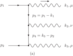
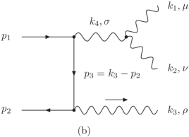
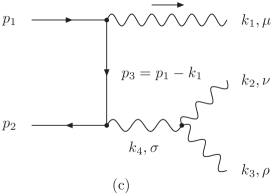
Figure 1: Diagram (a) represents the contributions from abelian interaction terms and diagrams (b) and (c) represent contributions from the non-abelian interaction terms.

The amplitudes were calculated using the Feynman rules in Ref.NcQED . We computed the helicity amplitudes with the aid of the symbolic manipulation program FORM and simplified the results using Mathematica.

To simplify the presentation of the results, we introduce kinematical variables

$$a=k_{2}\!\cdot\!k_{3}b = k_{3}\!\cdot\!k_{1}c=k_{1}\!\cdot\!k_{2}$$ (4)

$$p=p_{1}\!\cdot\!k_{1}q = p_{1}\!\cdot\!k_{2}r=p_{1}\!\cdot\!k_{3}$$ (5)

$$s=p_{2}\!\cdot\!k_{1}t = p_{2}\!\cdot\!k_{2}u=p_{2}\!\cdot\!k_{3}$$ (6)

$$v=\cos\left(k_{1}\!\cdot\!\theta\!\cdot\!k_{2}/2\right) w=\sin\left(k_{1}\!\cdot\!\theta\!\cdot\!k_{2}/2\right)$$ (7)

$$S = \left(p_{1}+p_{2}\right)^{2}\,,$$ (8)

where $p\!\cdot\!\theta\!\cdot\!q=p_{\mu}\theta^{\mu\nu}q_{\nu}$. These variables are related as

$$\begin{array}[]{rcccl}S/2&=&s+t+u&=&p+q+r\\ a&=&q+r-s&=&t+u-p\\ b&=&p+r-t&=&s+u-q\\ c&=&p+q-u&=&s+t-r\ .\end{array}$$ (9)

In the center of mass system we also have

$$k_{1}\!\cdot\!\theta\!\cdot\!k_{2}=k_{2}\!\cdot\!\theta\!\cdot\!k_{3}=k_{3}\!\cdot\!\theta\!\cdot\!k_{1}\ .$$ (10)

While there are only five independent variables, it is convenient for displaying the results and examining symmetries to retain six. If the helicities are labelled $\lambda,\bar{\lambda};\lambda_{1},\lambda_{2},\lambda_{3}$, the square of helicity amplitude $+,-;+,+,-$ is

$$\left|\mathcal{M}_{+,-;+,+,-}\right|^{2} = \frac{2\,e^{6}\,r^{2}}{p\,q\,s\,t}\bigg{[}S-4\,w^{2}\,\bigg{(}\frac{3\,S}{2}+\frac{a\,\left(p^{2}+s^{2}\right)}{b\,c}+\frac{b\,\left(q^{2}+t^{2}\right)}{a\,c}+\frac{c\,\left(r^{2}+u^{2}\right)}{a\,b}$$ (11)

$$- \frac{p\,q+\left(p+s\right)\,\left(q+t\right)+s\,t}{c}-\frac{p\,r+\left(p+s\right)\,\left(r+u\right)+s\,u}{b}-\frac{q\,r+\left(q+t\right)\,\left(r+u\right)+t\,u}{a}\bigg{)}$$

$$- 4\,v\,w\,\left(\frac{1}{a}+\frac{1}{b}+\frac{1}{c}\right)\epsilon(k_{1},k_{2},p_{1},p_{2})\bigg{]}\ .$$

The remaining squared amplitudes are given in Appendix C.

With the aid of Eqs. (4,5,6,7, and 10), it is easy to check that Eq. (11) satisfies Bose symmetry. The last term in Eq. (11) changes sign under the exchange of $p_{1}$ and $p_{2}$, which is a reflection of the lack of charge conjugation symmetry. The parity transformation $\vec{p}\to-\vec{p}$, $\lambda\to-\lambda$ gives $\mathcal{M}_{\lambda,\bar{\lambda};\lambda_{1},\lambda_{2},\lambda_{3}}=\mathcal{M}_{-\lambda,-\bar{\lambda};-\lambda_{1},-\lambda_{2},-\lambda_{3}}$, as can be seen using Appendix C. As a consequence, CP is violated, but CPT is preserved CPT . The CP violating terms cancel in the sum over fermion helicities.

Summing over photon helicities and averaging over electron helicities gives

$$\left|\mathcal{M}_{e^{+}e^{-}\rightarrow\gamma\gamma\gamma}\right|^{2} = e^{6}\,\frac{p\,s\,\left(p^{2}+s^{2}\right)+q\,t\,\left(q^{2}+t^{2}\right)+r\,u\,\left(r^{2}+u^{2}\right)}{p\,q\,r\,s\,t\,u}$$ (12)

$$\times \bigg{[}S-4\,w^{2}\,\bigg{(}\frac{a\,\left(p^{2}+s^{2}\right)}{b\,c}+\frac{b\,\left(q^{2}+t^{2}\right)}{a\,c}+\frac{c\,\left(r^{2}+u^{2}\right)}{a\,b}-\frac{p\,q+\left(p+s\right)\,\left(q+t\right)+s\,t}{c}$$

$$- \frac{p\,r+\left(p+s\right)\,\left(r+u\right)+s\,u}{b}-\frac{q\,r+\left(q+t\right)\,\left(r+u\right)+t\,u}{a}+\frac{3\,S}{2}\bigg{)}\bigg{]}.$$

We have checked that this result satisfies the Ward identity $\mathcal{M}_{\mu}k_{i}^{\mu}=0$ for each photon and that it reduces to the standard QED result CGTW if $\theta^{\mu\nu}=0$. space

III Cross Section Results

III.1 Unpolarized Cross Section

The details of obtaining the cross section from $|\mathcal{M}_{e^{+}e^{-}\rightarrow\gamma\gamma\gamma}|^{2}$, Eq. (12), are given in Appendix A. The result consists of the pure QED cross section, which contains an infrared divergence that must be regularized, and an infrared finite NCQED correction. To check the validity of our helicity amplitudes, we recalculated the QED spin averaged total cross section by retaining all terms linear in the electron mass squared, $m^{2}$, in the numerators of Eq. (12). Our result then agrees with that of Berends and Kleiss Berends , namely

$$\sigma^{QED}_{e^{+}e^{-}\rightarrow\gamma\gamma\gamma}=\frac{2\alpha^{3}}{S}\left(\left(\log\rho-1\right)^{2}\left(\log\omega-1\right)+3\right)\,,$$ (13)

with

$$\rho=\frac{S}{m^{2}}\ \ \ \omega=\frac{E^{2}}{E_{\rm min}^{\,2}}\,.$$ (14)

By assuming the non-commutative factor $w^{2}$ in Eq. (12) is small, we have $w^{2}=\sin^{2}\!\!\varphi\cong\varphi^{2}$, where $\varphi$ is

$$\varphi\equiv{\textstyle\frac{1}{2}}k_{1}\!\cdot\!\theta\!\cdot\!k_{2}={\textstyle\frac{1}{2}}\left(\vec{k_{1}}\times\vec{k_{2}}\right)\!\cdot\!\vec{\theta}\,.$$ (15)

It is then possible to express the non-commutative effects in terms of $\lambda$, the angle between $\vec{p}_{1}$ and $\vec{\theta}$ and $z=S/\Lambda_{NC}^{2}$. The NCQED contribution to the spin averaged cross section has the form

$$\sigma^{NCQED}_{e^{+}e^{-}\rightarrow\gamma\gamma\gamma}=\frac{z^{2}\alpha^{3}}{S}\left[\frac{2231}{720}-\frac{\pi^{2}}{120}-\frac{5}{2}\zeta(3)+\sin^{2}\lambda\left(\frac{\pi^{2}}{80}+\frac{7}{2}\zeta(3)-\frac{148957}{34560}-\frac{7\log\!\rho}{960}\right)\right]\,.$$ (16)

If we average over $\lambda$, the expression for the total cross section becomes

$$\sigma_{e^{+}e^{-}\rightarrow\gamma\gamma\gamma}=\frac{\alpha^{3}}{S}\bigg{[}2\left(\log\rho-1\right)^{2}\left(\log\omega-1\right)+6+z^{2}\left(\frac{65219}{69120}-\frac{\pi^{2}}{480}-\frac{3}{4}\zeta(3)-\frac{7\log\!\rho}{1920}\right)\bigg{]}\,.$$ (17)

With or without the average over $\lambda$, the effect of non-commutativity on spin averaged total cross section is relatively small since it depends on $z^{2}$ and has a $\log\rho$ rather than a $\log^{2}\rho$ dependence.

To determine if NCQED can be tested using the spin averaged three photon process, we examined the dependence of the cross section on the azimuthal angle $\phi$ of one of the photons. This is a pure NCQED effect since the QED cross section has no such $\phi$-dependence. Before doing this, it is important to determine the range of validity of the approximation $\sin^{2}\varphi\approx\varphi^{2}$. From Appendix A, $\varphi^{2}$ has the form

$$\varphi^{2}=\frac{z^{2}}{64}\nu_{1}^{2}\nu_{2}^{2}\sin^{2}\alpha\sin^{2}\beta\,,$$ (18)

where $\nu_{i}=E_{i}/E$ and $\alpha$ and $\beta$ vary between $0$ and $\pi$. Thus, the approximation is always good if $z<8$. Since all the other factors vary between $0$ and $1$, and we integrate over some or all of them in calculating the distributions, a limit on $z$ based on the the average value $\left\langle\varphi^{2}\right\rangle$ can be useful. This limit is

$$z<\frac{8}{\sqrt{\left\langle\nu_{1}^{2}\nu_{2}^{2}\sin^{2}\alpha\sin^{2}\beta\right\rangle}}<35\,.$$ (19)

In the following, we choose $\sqrt{S}=0.5\,\mathrm{TeV},\,1.0\,\mathrm{TeV},\,5.0\,\mathrm{TeV}$, which, for $\Lambda_{NC}=1.0\,\mathrm{TeV}$, corresponds to $z=0.25,1.0,25.0$.

As in the $e^{+}e^{-}\to\gamma\gamma$ case, the $\phi$-dependence of the spin averaged cross section is proportional to $z^{2}$. With no cut imposed on the polar angle $\theta$, we have

$$\frac{d\sigma}{d\phi} = \frac{z^{2}\alpha^{3}}{\pi S}\left[\frac{2231}{1440}-\frac{\pi^{2}}{240}-\frac{5}{4}\zeta(3)-\sin^{2}\lambda\left(\frac{86141}{69120}-\frac{11\pi^{2}}{1440}+\frac{7\log\rho}{1152}-\zeta(3)\right.\right.$$ (20)

$$+ \left.\left.\left(\frac{1963}{1080}+\frac{\pi^{2}}{360}-\frac{7\log\rho}{1440}-\frac{3}{2}\zeta(3)\right)\cos^{2}\phi\right)\right]\,.$$

The effect of this characteristic $\phi$-dependence is illustrated in the left panel of Fig 2.

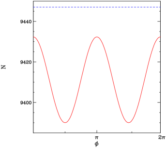
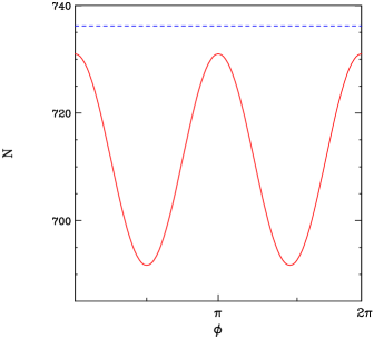
Figure 2: (color online) In the left panel, the solid line is number of events as a function of $\phi$ for the case $\sqrt{S}=5$ TeV, $\Lambda_{NC}=1$ TeV, $\lambda=\pi/4$, $\mathcal{L}=500$ fb^-1 and no cut on $\cos\theta$. The dashed line is the uniform background from QED with no $\cos\theta$ cut. The right panel shows the effect of imposing the additional cut $|\cos\theta|\leq 0.9$.

The signature of $3\gamma$ $\phi$-dependence, a unique feature of NCQED, can be further enhanced by imposing a cut on polar angle $\theta$. This has a rather large effect on the NCQED signal since the QED contribution to the $e^{+}e^{-}\to\gamma\gamma\gamma$ cross section is very sharply peaked in the forward a backward directions. The result of the cut $|\cos\theta|\leq 0.9$ is shown in the right panel of Fig 2.

We also checked the NCQED corrections to the QED energy and polar angle distributions of one of the photons. While there are some differences in the shapes of the NCQED distributions relative to their QED counterparts, particularly in the energy distribution, using these differences as a test of NCQED appears difficult because of their $z^{2}$ and energy dependence. The search for $\phi$-dependence remains the best possibility if the $e^{+}$ and $e^{-}$ beams are unpolarized.

There are, however, CP violating terms linear in $z$ in the individual helicity amplitudes, as can be seen in Eq. (11) or in Appendix C. To probe these terms it is necessary to consider polarization effects.

III.2 Polarized Cross Sections

We will confine our discussion to cross sections arising from longitudinally polarized beams. In this case, a typical cross section can be written m-p

$$\sigma_{P_{e^{-}}P_{e^{+}}} = \frac{1}{4}\left[(1+P_{e^{-}})(1+P_{e^{+}})\,\sigma_{RR}+(1-P_{e^{-}})(1-P_{e^{+}})\,\sigma_{LL}\right.$$ (21)

$$\hskip 4.0pt\left.+(1+P_{e^{-}})(1-P_{e^{+}})\,\sigma_{RL}+(1-P_{e^{-}})(1+P_{e^{+}})\,\sigma_{LR}\right]\,,$$

where, for example, $\sigma_{RL}$ denotes the cross section when the $e^{-}$ beam has pure right-handed polarization ($P_{e^{-}}=1$) and the $e^{+}$ beam has pure left-handed polarization ($P_{e^{+}}=-1$). The remaining cross sections are defined similarly.

For the process $e^{+}e^{-}\to\gamma\gamma\gamma$, amplitudes with $\lambda=\bar{\lambda}$ vanish, and we can express the polarized cross section as m-p

$$\sigma_{P_{e^{-}}P_{e^{+}}} = (1-P_{e^{-}}P_{e^{+}})\frac{\sigma_{RL}+\sigma_{LR}}{4}\left[1-\frac{P_{e^{-}}-P_{e^{+}}}{1-P_{e^{-}}P_{e^{+}}}\frac{\sigma_{LR}-\sigma_{RL}}{\sigma_{LR}+\sigma_{RL}}\right]$$ (22)

$$= (1-P_{e^{-}}P_{e^{+}})\sigma_{\rm unpol}\left[1-P_{\rm eff}A_{LR}\right]\,,$$

where the effective polarization $P_{\rm eff}$ and the left-right asymmetry $A_{LR}$ are

$$P_{\rm eff} = \frac{P_{e^{-}}-P_{e^{+}}}{1-P_{e^{-}}P_{e^{+}}}\,,$$ (23)

$$A_{LR} = \frac{\sigma_{LR}-\sigma_{RL}}{\sigma_{LR}+\sigma_{RL}}\,.$$ (24)

The left-right asymmetry can be obtained using the squared amplitudes in Appendix C and Eq.(̇17), which results in

$$A_{LR}=-\frac{E_{e}^{2}\cos\lambda}{\Lambda_{NC}^{2}}\frac{\mbox{\rule[-10.0pt]{0.0pt}{26.0pt}}\Big{(}4\zeta(3)-\displaystyle{\frac{29}{6}}+\displaystyle{\frac{4\pi^{2}}{9}}\Big{)}}{\Big{[}\mbox{\rule[-10.0pt]{0.0pt}{26.0pt}}(\log(\displaystyle{\frac{4E_{e}^{2}}{m^{2}}})-1)^{2}(\log(\omega)-1)+3\Big{]}}\,.$$ (25)

For the process $e^{+}e^{-}\to\gamma\gamma\gamma$, the NCQED correction is the main source of a left-right asymmetry. Competing standard model sources of left-right asymmetry such as $Z$ exchange in Möller scattering HPR are suppressed because they involve loops. Taking $\Lambda_{NC}=1.0$ TeV, Table 1 shows the cross section values for the cases HPR $P_{e^{-}}=-P_{e^{+}}=\pm 0.9$ and several values of $\sqrt{s}$ and $\cos\lambda=1$.

$\sqrt{s}$ TeV	$\sigma_{0.9\,-0.9}$ fb	$\sigma_{-0.9\,0.9}$ fb
1.0	$4315.4$	$4316.9$
2.0	$1187.9$	$1189.3$
3.0	$557.1$	$558.6$
4.0	$325.1$	$326.6$
5.0	$213.9$	$215.4$

Table 1: The cross sections for 90% left-right and right-left polarized beams are shown for $\Lambda_{NC}=1$ TeV and $\lambda=0$.

As the numbers in the Table 1 indicate, the left-right asymmetry, though non-zero, must be distinguished from a fluctuation in the large left-right symmetric QED $e^{+}e^{-}\to\gamma\gamma\gamma$ cross section. To obtain a sense of the range of values of $\Lambda_{NC}$ that can be probed polarized cross sections, we examined the signal to square root of background ratio

$$R=\frac{\mathcal{L}(\sigma_{0.9\,-0.9}-\sigma_{-0.9\,0.9})}{\sqrt{\displaystyle\mathcal{L}(\sigma_{0.9\,-0.9}+\sigma_{-0.9\,0.9})}}\,.$$ (26)

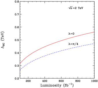
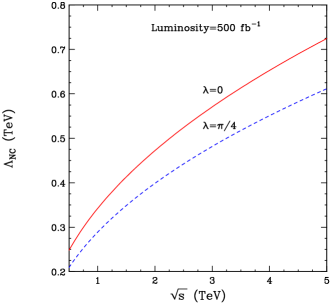
Figure 3: (color online) The bounds on $\Lambda_{NC}$ attainable using the left-right asymmetry of the total cross section are illustrated as a function of luminosity at $\sqrt{S}=2$ TeV (left) and as a function of $\sqrt{S}$ for $\mathcal{L}=500\,\mathrm{fb}^{-1}$ (right). The solid lines correspond to $\lambda=0$ and the dashed lines to $\lambda=\pi/4$.

Requiring $R\geq 3$ implies the bounds attainable on $\Lambda_{NC}$ illustrated in Fig. 3 as function of luminosity $\mathcal{L}$ and collider energy $\sqrt{S}$.

The constraints on $\Lambda_{NC}$ obtainable from the polarized total cross section suggest that cuts on the polarization asymmetries in distributions such as

$$\frac{\mbox{\rule[-4.0pt]{0.0pt}{14.0pt}}\displaystyle(d\sigma_{LR}-d\sigma_{RL})/d\nu}{\mbox{\rule[-4.0pt]{0.0pt}{14.0pt}}\displaystyle(d\sigma_{LR}+d\sigma_{RL})/d\nu}\quad\mathrm{or}\quad\frac{\mbox{\rule[-4.0pt]{0.0pt}{14.0pt}}\displaystyle(d\sigma_{LR}-d\sigma_{RL})/d\cos\theta}{\mbox{\rule[-4.0pt]{0.0pt}{14.0pt}}\displaystyle(d\sigma_{LR}+d\sigma_{RL})/d\cos\theta}$$ (27)

could improve the bounds on $\Lambda_{NC}$. These distributions are shown in Fig. 4.

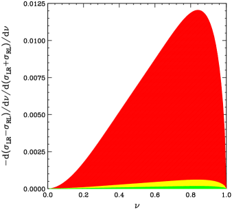
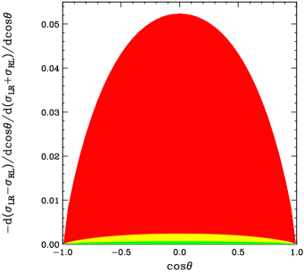
Figure 4: (color online) The polarization asymmetries with respect to the photon energy fraction $\nu$ (left) and the photon angle with respect to the beam axis (right) are shown. The three shaded regions correspond to center of mass energies of 0.5, 1.0 and 5.0 TeV.

While both distributions show a distinct left-right asymmetry, the $\cos\theta$ distribution is the most promising from the experimental point of view in that it can be rather large – $\sim\;\mathrm{few}\;$% – over a substantial region of $\cos\theta$. By imposing cuts on $\cos\theta$ it is possible substantially increase the lower bound on $\Lambda_{NC}$ obtained using Eq. (26). The largest lower bound is obtained by restricting $\cos\theta$ as $|\cos\theta|\leq 0.85$, which is illustrated in Fig. (5).

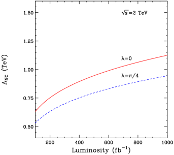
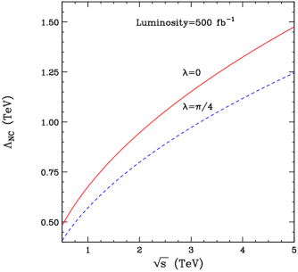
Figure 5: (color online) Same as Fig. 3 with $|\cos\theta|\leq 0.85$.

The behavior of the bound on $\Lambda_{NC}$ as the cut on $\cos\theta$ varies from $|\cos\theta|\leq 0.5$ to $|\cos\theta|\leq 1.0$ is shown in Fig. 6.

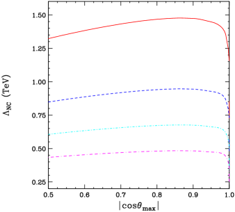
Figure 6: (color online) The bounds on $\Lambda_{NC}$ for $0.5\leq|\cos\theta_{\rm max}|\leq 1.0$ are shown for $\sqrt{S}=0.5\,\mathrm{TeV}$ (dot-dash-dash), 1.0 TeV (dot-dash), 2.0 TeV (dashed) and 5.0 TeV (solid). Here $\mathcal{L}=500\,\mathrm{fb}^{-1}$ and $\cos\lambda=1$. The bounds scale as $\mathcal{L}^{1/4}$ and $\sqrt{\cos\lambda}$.

IV Discussion and Conclusions

To summarize, we have computed the noncommutative contributions to the angular and energy distributions of a single photon as well as to the total cross section for the process $e^{+}e^{-}\to\gamma\gamma\gamma$ assuming both the unpolarized and polarized electron and positron beams. Because we are dealing with a three particle final state, it is possible to include these corrections using only the space-space portion of the tensor $\theta^{\mu\nu}$. This enables us to avoid the use of the space-time terms $\theta^{k0}$ and thereby satisfy the requirement of unitarity Chai . The use of space-time terms cannot be always avoided in $2\to 2$ processes e.g. $e\gamma\to e\gamma$, $e^{+}e^{-}\to\gamma\gamma$ or $e^{+}e^{-}\to e^{+}e^{-}$ and this tends to complicate their interpretation. The cross sections and distributions depend on the angle $\lambda$ between the beam direction and the non-commutativity vector $\vec{\theta}$. In the unpolarized case, the noncommutative effects are second order in the ratio $z=S/\Lambda_{NC}^{2}$, whereas in polarized case, the noncommutative effects are leading order in $z$.

In the unpolarized case, the shapes of the QED and NCQED energy distributions are quite different but it is the dependence of the cross section on the azimuthal angle $\phi$ which offers the best opportunity to detect non-commutative effects. The observation of any variation of the cross section with respect to $\phi$ is a clear violation of Lorentz symmetry. It is possible to introduce reasonable cuts significantly enhance this signature of non-commutativity.

Further, the use of polarized beams makes it possible to probe the order $z$ CP violating terms in the helicity amplitudes by measuring the left-right asymmetry. In contrast to Möller scattering, where $Z$ exchange introduces a large standard model left-right asymmetry which competes with the NCQED asymmetry, the NCQED left-right asymmetry in the $3\gamma$ final state is the dominant source of asymmetry, with standard model contributions being suppressed by loops. Even without cuts on the polarized cross section, the bounds attainable on $\Lambda_{NC}$ are competitive with those obtained in pair annihilation HPR . Imposition of cuts on $\cos\theta$, the angle between one of the photons and the beam direction, extends the reach on $\Lambda_{NC}$ to the TeV range. Accumulating enough data to reach these bounds will require monitoring the (unknown) direction of the non-commutativity vector $\vec{\theta}$. Techniques for doing this were proposed by Hewett, Petriello and Rizzo HPR and implemented by the OPAL collaboration Abbiendi .

Currently, the experimental lower bound on $\Lambda_{NC}$ is $140$ GeV Abbiendi , and the calculations of Ref  HPR indicate that $\Lambda_{NC}$ scales of $1.7$ TeV can be probed in Möller scattering at a $500$ Gev $e^{+}e^{-}$ collider. Like Möller scattering, the NCQED contribution to $e^{+}e^{-}\to\gamma\gamma\gamma$ can be parameterized solely in terms of the unitarity preserving space-space components of $\theta^{\mu\nu}$. This, together with its NCQED dominant left-right asymmetry signature, makes the three photon process promising candidate in the experimental search for noncommutative effects.

Appendix A Spin Averaged Cross Section

The tensor $\theta_{ij}$ can be parameterized in terms of a unit vector $\vec{\theta}$ and a noncommutativity scale $\Lambda_{NC}$ as

$$\theta_{ij}=\frac{1}{\Lambda_{NC}^{2}}\epsilon_{ijk}\theta^{k}\,.$$ (28)

To define the coordinates, we fix the origin at the center of mass, choose the z axis parallel to $\vec{p_{1}}$ and take $\vec{\theta}$ in the plane x-z plane. In this system, $\vec{k_{1}}$ is defined by its polar angle $\alpha_{1}$, its azimuthal the angle $\beta_{1}$ and its energy $E_{1}$. Similarly $\vec{k_{2}}$ is defined by its energy $E_{2}$, its polar angle $\alpha_{2}$ and, for convenience, an azimuthal angle $\beta_{1}+\beta_{2}$.

The phase space integration is given in detail in Appendix B, where it is shown that, in addition to the variables mentioned above, it is necessary to introduce a minimum photon energy $E_{\rm min}$ to control the infrared singularities. Introducing the dimensionless variables ($i=1,2$)

$$\nu_{i}=\frac{E_{i}}{E} c_{i}=\cos{\alpha_{i}}$$

$$\epsilon=\frac{E_{\rm min}}{E} n=\sqrt{1-\frac{m^{2}}{E^{2}}}\,,$$ (29)

the terms in Eq.(12) can be expressed as

$$\begin{array}[]{ccc}\mbox{\rule[-10.0pt]{0.0pt}{26.0pt}}p=\frac{S}{4}\nu_{1}\left(1-nc_{1}\right)&q=\frac{S}{4}\nu_{2}\left(1-nc_{2}\right)&r=\frac{S}{4}\left(2-\nu_{1}\left(1-nc_{1}\right)-\nu_{2}\left(1-nc_{2}\right)\right)\\ \mbox{\rule[-10.0pt]{0.0pt}{26.0pt}}s=\frac{S}{4}\nu_{1}\left(1+nc_{1}\right)&t=\frac{S}{4}\nu_{2}\left(1+nc_{2}\right)&u=\frac{S}{4}\left(2-\nu_{1}\left(1+nc_{1}\right)-\nu_{2}\left(1+nc_{2}\right)\right)\end{array}\,.$$ (30)

The total cross section is expressible in terms of these variables as

$$\sigma_{e^{+}e^{-}\rightarrow\gamma\gamma\gamma} = \frac{1}{6\,(4\pi)^{5}}\left(\int^{1-\epsilon}_{\epsilon}\mathrm{d}\nu_{1}\int^{1}_{1-\nu_{1}}\mathrm{d}\nu_{2}+\int^{1}_{1-\epsilon}\mathrm{d}\nu_{1}\int^{2-\nu_{1}-\epsilon}_{\epsilon}\mathrm{d}\nu_{2}\right)$$ (31)

$$\times \int^{1}_{-1}\mathrm{d}c_{1}\int^{c_{+}}_{c_{-}}\mathrm{d}c_{2}\int^{2\pi}_{0}\mathrm{d}\beta_{1}\ \frac{\left|\mathcal{M}_{e^{+}e^{-}\rightarrow\gamma\gamma\gamma}\right|^{2}}{\sqrt{\left(c_{+}-c_{2}\right)\left(c_{2}-c_{-}\right)}}$$

where

$$c_{\pm}=c_{1}-2\frac{c_{1}\left(\nu_{1}+\nu_{2}-1\right)\mp\sqrt{\left(1-c_{1}^{2}\right)\left(1-\nu_{1}\right)\left(1-\nu_{2}\right)\left(\nu_{1}+\nu_{2}-1\right)}}{\nu_{1}\nu_{2}}.$$ (32)

Using the symmetry of Eq.(12) under a permutation of $\vec{k_{1}},\vec{k_{2}},\vec{k_{3}}$, and neglecting $m^{2}$ in the numerator of Eq. (12), the commutative contribution to the cross section becomes

$$\sigma^{QED}_{e^{+}e^{-}\rightarrow\gamma\gamma\gamma} = \frac{2\alpha^{3}}{S\,\pi}\left(\int^{1-\epsilon}_{\epsilon}\mathrm{d}\nu_{1}\int^{1}_{1-\nu_{1}}\mathrm{d}\nu_{2}+\int^{1}_{1-\epsilon}\mathrm{d}\nu_{1}\int^{2-\nu_{1}-\epsilon}_{\epsilon}\mathrm{d}\nu_{2}\right)\int^{1}_{-1}\mathrm{d}c_{1}\int^{c_{+}}_{c_{-}}\mathrm{d}c_{2}$$ (33)

$$\times \frac{\left(2-\nu_{1}-\nu_{2}\right)^{2}+n^{2}\left(c_{1}\nu_{1}+c_{2}\nu_{2}\right)^{2}}{\left(1-n^{2}c_{1}^{2}\right)\left(1-n^{2}c_{2}^{2}\right)\sqrt{\left(c_{+}-c_{2}\right)\left(c_{2}-c_{-}\right)}\ \nu_{1}^{2}\nu_{2}^{2}}\,,$$

where the integration over $\beta_{1}$ has been completed since the process has axial symmetry for $\vec{\theta}=0$. The integration of Eq.(33), neglecting terms which vanish for $m^{2}/S\rightarrow 0$, gives GT

$$\sigma^{QED}_{e^{+}e^{-}\rightarrow\gamma\gamma\gamma}=\frac{2\alpha^{3}}{S}\left(\left(\log\rho-1\right)^{2}\left(\log\omega-1\right)+\left(\log\rho-1\right)\log\omega+3-\frac{\pi^{2}}{3}\right)$$ (34)

with

$$\rho=\frac{S}{m^{2}}\ \ \ \omega=\frac{E^{2}}{E_{\rm min}^{\,2}}\,.$$ (35)

As will be seen below, the NCQED correction is small relative to the pure QED cross section. To be certain that the comparison of the two is sensible, we computed the correction to the QED cross section obtained by retaining all the order $m^{2}$ terms in the numerators of Eq. (12). The calculations are explained in Berends ; Eidelman ; Fujimoto . Our result, which agrees with that of Berends and Kleiss, is

$$\sigma^{QED}_{e^{+}e^{-}\rightarrow\gamma\gamma\gamma}=\frac{2\alpha^{3}}{S}\left(\left(\log\rho-1\right)^{2}\left(\log\omega-1\right)+3\right)$$ (36)

For the noncommutative term, the integrand is no longer invariant with respect to rotations about the z axis and it is necessary to consider the $\beta_{1}$ integration in more detail. From Eq.(28) we have

$$\varphi \equiv {\textstyle\frac{1}{2}}k_{1}\!\cdot\!\theta\!\cdot\!k_{2}={\textstyle\frac{1}{2}}\left(\vec{k_{1}}\times\vec{k_{2}}\right)\!\cdot\!\vec{\theta}$$ (37)

$$= \frac{E_{1}E_{2}}{2\Lambda_{NC}^{2}}\,\ \left(\sin{\alpha_{1}}\left(\sin{\beta_{1}}\cos{\alpha_{2}}\sin\lambda+\sin{\alpha_{2}}\sin{\beta_{2}}\cos\lambda\right)-\cos{\alpha_{1}}\sin{\alpha_{2}}\sin{\left(\beta_{1}+\beta_{2}\right)}\sin\lambda\right)\,,$$

where $\lambda$ is the angle between $\vec{p_{1}}$ and $\vec{\theta}$. Assuming $\varphi$ to be small, the noncommutative factor $w^{2}$ in Eq.(̇12) becomes $w^{2}=\sin^{2}\!\!\varphi\cong\varphi^{2}$. Since $\beta_{1}$ appears only in $w^{2}$ we can integrate this factor to obtain

$$\int^{2\pi}_{0}\mathrm{d}\beta_{1}\,\varphi^{2} = \frac{\pi z^{2}}{64}\left[(1-3\cos^{2}\lambda)\left(4\,c_{1}c_{2}(\nu_{1}+\nu_{2}-1)+\nu_{1}\nu_{2}(c_{1}-c_{2})^{2}\right)\right.$$ (38)

$$\left.\hskip 24.0pt+8\,\cos^{2}\lambda(1-\nu_{1})(1-\nu_{2})(\nu_{1}+\nu_{2}-1)\right]\,.$$

Owing to the additional factors of $E_{1}$ and $E_{2}$ in Eq.(37), the noncommutative contribution is infrared finite, and it is possible to set $\epsilon=0$ in Eq. (31). Then, using Eq.(38) and the symmetry of Eq.(12) in $k_{1},k_{2},k_{3}$, the expression for the noncommutative contribution to the cross section is

$$\sigma^{NCQED}_{e^{+}e^{-}\rightarrow\gamma\gamma\gamma}=-\frac{z^{2}\alpha^{3}}{64\,\pi\,S}\int^{1}_{0}\mathrm{d}\nu_{1}\int^{1}_{1-\nu_{1}}\mathrm{d}\nu_{2}\int^{1}_{-1}\mathrm{d}c_{1}\int^{c_{+}}_{c_{-}}\mathrm{d}c_{2}\frac{\mathcal{N}(c_{1},c_{2},\nu_{1},\nu_{2})}{\mathcal{D}(c_{1},c_{2},\nu_{1},\nu_{2})}\,,$$ (39)

where

$$\mathcal{N}(c_{1},c_{2},\nu_{1},\nu_{2}) = \left[(2-\nu_{1}-\nu_{2})^{2}+n^{2}(c_{1}\nu_{1}+c_{2}\nu_{2})^{2}\right]\left[\left(3\left(\nu_{1}+\nu_{2}\right)-1\right)\left(2-\nu_{1}\nu_{2}\right)-\nu_{1}^{2}\nu_{2}^{2}\right.$$

$$+ \left.(2\nu_{1}\nu_{2}-7)(\nu_{1}+\nu_{2})^{2}+4(\nu_{1}+\nu_{2})^{3}-(\nu_{1}+\nu_{2})^{4}+n^{2}\left(c_{1}c_{2}\nu_{1}\nu_{2}(\nu_{1}^{2}+\nu_{1}\nu_{2}+\nu_{2}^{2}-1)\right.\right.$$

$$+ \left.\left.c_{1}^{2}\nu_{1}^{2}(1-\nu_{2}+\nu_{1}^{2}+\nu_{1}\nu_{2}+\nu_{2}^{2}-2\nu_{1})+c_{2}^{2}\nu_{2}^{2}(1-\nu_{1}+\nu_{1}^{2}+\nu_{1}\nu_{2}+\nu_{2}^{2}-2\nu_{2})\right)\right]$$

$$\times \left[(1-3c_{\lambda}^{2})\nu_{1}\nu_{2}\left(4c_{1}c_{2}(\nu_{1}+\nu_{2}-1)+\nu_{1}\nu_{2}(c_{1}-c_{2})^{2}\right)+8\,c_{\lambda}^{2}(1-\nu_{1})(1-\nu_{2})(\nu_{1}+\nu_{2}-1)\right]\,,$$

and

$$\mathcal{D}(c_{1},c_{2},\nu_{1},\nu_{2})=\nu_{1}^{2}\nu_{2}^{2}\left(1-\nu_{1}\right)\left(1-\nu_{2}\right)\left(\nu_{1}+\nu_{2}-1\right)\left(1-n^{2}c_{1}^{2}\right)\left(1-n^{2}c_{2}^{2}\right)\sqrt{\left(c_{+}-c_{2}\right)\left(c_{2}-c_{-}\right)}\,.$$ (41)

When Eq.(39) is integrated over $\alpha_{1}$ and $\alpha_{2}$, we can take $\rho=m^{2}/S=0$ except for terms involving $\log\rho$, and take $n=1$ in Eq. (A), which does not introduce any collinear divergences. The integration of Eq.(39) can be evaluated analytically and the noncommutative contribution is

$$\sigma^{NcQED}_{e^{+}e^{-}\rightarrow\gamma\gamma\gamma}=\frac{z^{2}\alpha^{3}}{S}\left[\frac{2231}{720}-\frac{\pi^{2}}{120}-\frac{5}{2}\zeta(3)+\sin^{2}\lambda\left(\frac{\pi^{2}}{80}+\frac{7}{2}\zeta(3)-\frac{148957}{34560}-\frac{7\log\!\rho}{960}\right)\right]\,.$$ (42)

From this expression it is clear that production of the three photons depends on the angle between the incident beam and the vector $\vec{\theta}$, which violates Lorentz invariance. Since the direction of $\vec{\theta}$ is not known, we average over $\sin^{2}\lambda$ to obtain

$$\bar{\sigma}^{NCQED}_{e^{+}e^{-}\rightarrow\gamma\gamma\gamma}=\frac{z^{2}\alpha^{3}}{S}\left(\frac{65219}{69120}-\frac{\pi^{2}}{480}-\frac{3}{4}\zeta(3)-\frac{7\log\!\rho}{1920}\right)\,.$$ (43)

Adding Eq.(34) and Eq.(43) we get the total cross section

$$\sigma_{e^{+}e^{-}\rightarrow\gamma\gamma\gamma}=\frac{\alpha^{3}}{S}\bigg{[}2\left(\log\rho-1\right)^{2}\left(\log\omega-1\right)+6+z^{2}\left(\frac{65219}{69120}-\frac{\pi^{2}}{480}-\frac{3}{4}\zeta(3)-\frac{7\log\!\rho}{1920}\right)\bigg{]}\,.$$ (44)

Appendix B Phase Space

Taking the center of mass energies of the electron and positron to be $E$ and the flux factor $\left|\vec{v_{1}}-\vec{v_{2}}\right|\to 2$, the expression for the three body phase space in the electron-positron center of mass is

$$\mathrm{d}\Gamma = \frac{\left(2\pi\right)^{4}}{3!\,2\left(4E^{2}\right)}\delta^{4}\!\left(p_{1}+p_{2}-k_{1}-k_{2}-k_{3}\right)\frac{\mathrm{d}^{3}\vec{k_{1}}}{\left(2\pi\right)^{3}2E_{1}}\frac{\mathrm{d}^{3}\vec{k_{2}}}{\left(2\pi\right)^{3}2E_{2}}\frac{\mathrm{d}^{3}\vec{k_{3}}}{\left(2\pi\right)^{3}2E_{3}}\,$$ (45)

$$= \frac{1}{3S\,(4\pi)^{5}}\delta\!\left(2E-E_{1}-E_{2}-E_{3}\right)\delta^{3}\!\left(\vec{k_{1}}+\vec{k_{2}}+\vec{k_{3}}\right)\frac{\mathrm{d}^{3}\vec{k_{1}}\mathrm{d}^{3}\vec{k_{2}}\mathrm{d}^{3}\vec{k_{3}}}{E_{1}E_{2}E_{3}}$$

where we have already introduced the symmetry factor $1/3!$. In spherical coordinates the components of $\vec{k_{1}}$ and $\vec{k_{2}}$ can be defined by

$$\vec{k_{1}} = E_{1}\left\{\sin{\alpha_{1}}\cos{\beta_{1}},\sin{\alpha_{1}}\sin{\beta_{1}},\cos{\alpha_{1}}\right\}\,$$

$$\vec{k_{2}} = E_{2}\left\{\sin{\alpha_{2}}\cos{\left(\beta_{1}+\beta_{2}\right)},\sin{\alpha_{2}}\sin{\left(\beta_{1}+\beta_{2}\right)},\cos{\alpha_{2}}\right\}\,.$$ (46)

The integration over $\delta^{3}\!\left(\vec{k_{1}}+\vec{k_{2}}+\vec{k_{3}}\right)$ gives

$$E_{3} = \sqrt{\vec{k_{3}}^{2}}=\sqrt{\left(\vec{k_{1}}+\vec{k_{2}}\right)^{2}}$$ (47)

$$= \sqrt{E_{1}^{2}+E_{2}^{2}+2E_{1}E_{2}\left(\cos{\alpha_{1}}\cos{\alpha_{2}}+\cos{\beta_{2}}\sin{\alpha_{1}}\sin{\alpha_{2}}\right)}$$

where we have used the definitions (B). The phase space integral Eq.(45) can then be written

$$\mathrm{d}\Gamma = \frac{\delta\!\left(2E-E_{1}-E_{2}-E_{3}\right)}{3S\,(4\pi)^{5}}\frac{\mathrm{d}^{3}\vec{k_{1}}\mathrm{d}^{3}\vec{k_{2}}}{E_{1}E_{2}E_{3}}$$ (48)

$$= \frac{\delta\!\left(2E-E_{1}-E_{2}-E_{3}\right)}{3S\,(4\pi)^{5}}\mathrm{d}E_{1}\mathrm{d}E_{2}\mathrm{d}\cos{\alpha_{1}}\mathrm{d}\cos{\alpha_{2}}\mathrm{d}\beta_{1}\mathrm{d}\beta_{2}\frac{E_{1}E_{2}}{E_{3}}$$

with $E_{3}$ given by Eq.(47). The remaining integration over $\delta\!\left(2E-E_{1}-E_{2}-E_{3}\right)$ leads to

$$E_{3}^{2} = E_{1}^{2}+E_{2}^{2}+2E_{1}E_{2}\left(\cos{\alpha_{1}}\cos{\alpha_{2}}+\cos{\beta_{2}}\sin{\alpha_{1}}\sin{\alpha_{2}}\right)$$ (49)

$$= \left(2E-E_{1}-E_{2}\right)^{2}\,.$$

Solving Eq.(49) for $\beta_{2}$ results in two solutions

$$\beta_{2}=\pm\beta_{20}$$ (50)

with

$$\beta_{20}=\arccos{\left(\frac{E_{1}E_{2}(1-\cos{\alpha_{1}}\cos{\alpha_{2}})-2E(E_{1}+E_{2}-E)}{E_{1}E_{2}\sin{\alpha_{1}}\sin{\alpha_{2}}}\right)}\,.$$ (51)

The derivative of the argument of the $\delta$ with respect to $\beta_{2}$,

$$\frac{d\left(2E-E_{1}-E_{2}-E_{3}\right)}{d\beta_{2}}=\frac{E_{1}E_{2}}{E_{3}}\sin{\alpha_{1}}\sin{\alpha_{2}}\sin{\beta_{2}}\,.$$ (52)

then gives

$$\delta\!\left(2E-E_{1}-E_{2}-E_{3}\right)=\frac{1}{\left|\displaystyle\frac{E_{1}E_{2}}{E_{3}}\sin{\alpha_{1}}\sin{\alpha_{2}}\sin{\beta_{20}}\right|}\left(\mbox{\rule[-10.0pt]{0.0pt}{26.0pt}}\delta(\beta_{2}-\beta_{20})+\delta(\beta_{2}+\beta_{20})\right)$$ (53)

Replacing the Eq.(53) in Eq.(48) we get

$$d\Gamma=\frac{1}{3S\,(4\pi)^{5}}\mathrm{d}E_{1}\mathrm{d}E_{2}\mathrm{d}\cos{\alpha_{1}}\mathrm{d}\cos{\alpha_{2}}\mathrm{d}\beta_{1}\mathrm{d}\beta_{2}\\ \frac{\delta\!\left(\beta_{2}-\beta_{20}\right)+\delta\!\left(\beta_{2}+\beta_{20}\right)}{\sin{\alpha_{1}}\sin{\alpha_{2}}\sin{\beta_{20}}}\,.$$

In the squared amplitude, $\beta_{2}$ is present only in the noncommutative factor $w^{2}$. As can be seen from Eq.(30), the other variables are independent of $\beta_{2}$. The integration over $\beta_{2}$ produces $w^{2}(\beta_{20})$ and $w^{2}(-\beta_{20})$, but these contributions are equal after the subsequent $\beta_{1}$ integration. Hence, for both the QED and NCQED terms, we can write

$$d\Gamma = \frac{2}{3S\,(4\pi)^{5}}\frac{\mathrm{d}E_{1}\,\mathrm{d}E_{2}\,\mathrm{d}\cos{\alpha_{1}}\,\mathrm{d}\cos{\alpha_{2}}\,\mathrm{d}\beta_{1}}{\sin{\alpha_{1}}\,\sin{\alpha_{2}}\,\sin{\beta_{2}}}\,,$$ (54)

where for simplicity we have dropped the zero on $\beta_{2}$. The limits of integration on, say, $\cos\alpha_{2}$ are constrained by Eq. (51). Using this equation to solve for $\sin\alpha_{1}\sin\alpha_{2}\sin\beta_{2}$, we find, in the notation of Eq. (A),

$$\sin{\alpha_{1}}\,\sin{\alpha_{2}}\,\sin{\beta_{2}}=\sqrt{(c_{+}-c_{2})(c_{2}-c_{-})}$$ (55)

with

$$c_{\pm}=c_{1}-2\frac{c_{1}\left(\nu_{1}+\nu_{2}-1\right)\mp\sqrt{\left(1-c_{1}^{2}\right)\left(1-\nu_{1}\right)\left(1-\nu_{2}\right)\left(\nu_{1}+\nu_{2}-1\right)}}{\nu_{1}\nu_{2}}.$$ (56)

The limits of integration on the energies are determined by solving the relations

$$E_{\rm min}\leq E_{j}\leq E\qquad E_{1}+E_{2}+E_{3}=2E\,,$$ (57)

with $j=1,2,3$, for $E_{1}$ and $E_{2}$. Elimination of $E_{3}$ yields the additional inequalities

$$E_{2}\geq E-E_{1}\,,\qquad\leq 2E-E_{1}-E_{\rm min}\,.$$ (58)

The limits of integration on $E_{2}$ depend on whether $E_{\rm min}\leq E_{1}\leq E-E_{\rm min}$ or $E-E_{\rm min}\leq E_{1}\leq E$. In the former case,

$$E-E_{1}\leq E_{2}\leq E\,,$$ (59)

while in the latter

$$E_{\rm min}\leq E_{2}\leq 2E-E_{1}-E_{\rm min}\,.$$ (60)

Appendix C Squared Modulus of the Helicity Amplitudes

The helicity amplitudes with permuted photon helicities can be derived by the corresponding permutation of the variables $p,q,r$ and $s,t,u$. Amplitudes with every helicity reversed just change the sign of CP-breaking term, while amplitudes in which the electron and positron are exchanged can be derived changing the sign of the antisymmetric term and exchanging the variables $p,q,r$ with $s,t,u$. The amplitudes $\{\pm,\pm;\lambda_{1},\lambda_{2},\lambda_{3}\}$ and $\{\lambda,\bar{\lambda};\pm,\pm,\pm\}$ are zero. The twelve non-zero helicity amplitudes are given in the following table.

$\lambda,\bar{\lambda};\lambda_{1},\lambda_{2},\lambda_{3}$	$|\mathcal{M}_{\lambda,\bar{\lambda};\lambda_{1},\lambda_{2},\lambda_{3}}|^{2}$	$\lambda,\bar{\lambda};\lambda_{1},\lambda_{2},\lambda_{3}$	$|\mathcal{M}_{\lambda,\bar{\lambda};\lambda_{1},\lambda_{2},\lambda_{3}}|^{2}$
$+,-;+,+,-$	$\displaystyle\frac{r^{2}}{pqst}\mathcal{A}_{-}$	$+,-;-,-,+$	$\displaystyle\frac{u^{2}}{pqst}\mathcal{A}_{-}$
$+,-;+,-,+$	$\displaystyle\frac{q^{2}}{prsu}\mathcal{A}_{-}$	$+,-;-,+,-$	$\displaystyle\frac{t^{2}}{prsu}\mathcal{A}_{-}$
$+,-;-,+,+$	$\displaystyle\frac{p^{2}}{qrtu}\mathcal{A}_{-}$	$+,-;+,-,-$	$\displaystyle\frac{s^{2}}{qrtu}\mathcal{A}_{-}$
$-,+;-,-,+$	$\displaystyle\frac{r^{2}}{pqst}\mathcal{A}_{+}$	$-,+;+,+,-$	$\displaystyle\frac{u^{2}}{pqst}\mathcal{A}_{+}$
$-,+;-,+,-$	$\displaystyle\frac{q^{2}}{prsu}\mathcal{A}_{+}$	$-,+;+,-,+$	$\displaystyle\frac{t^{2}}{prsu}\mathcal{A}_{+}$
$-,+;+,-,-$	$\displaystyle\frac{p^{2}}{qrtu}\mathcal{A}_{+}$	$-,+;-,+,+$	$\displaystyle\frac{s^{2}}{qrtu}\mathcal{A}_{+}$

Table 2: The absolute squares of the twelve non-zero helicity amplitudes, $|\mathcal{M}_{\lambda,\bar{\lambda};\lambda_{1},\lambda_{2},\lambda_{3}}|^{2}$, are expressed in terms of the amplitudes $\mathcal{A}_{\pm}$ given below.

The common factor $\mathcal{A}_{\pm}$ in all the entries in Table 2 is

$$\mathcal{A}_{\pm} = 2e^{6}\left[S-4w^{2}\left(\frac{3}{2}S+\frac{a\,(p^{2}+s^{2})}{bc}+\frac{b\,(q^{2}+t^{2})}{ac}+\frac{c\,(r^{2}+u^{2})}{ab}\right.\right.$$ (61)

$$\hskip 6.0pt-\left.\left.\frac{pq+(p+s)(q+t)+st}{c}-\frac{pr+(p+s)(r+u)+su}{b}-\frac{qr+(q+t)(r+u)+tu}{a}\right)\right.$$

$$\hskip 6.0pt\pm\left.4vw\left(\frac{1}{a}+\frac{1}{b}+\frac{1}{c}\right)\varepsilon(k_{1},k_{2},p_{1},p_{2}))\right]$$

References

- (1) H. S. Snyder, Phys. Rev. D 71, 38 (1947).
- (2) A. Connes, M. R. Douglas and A. Schwarz, JHEP 02, 003 (1998).
- (3) M. R. Douglas and C. Hull, JHEP 02, 008 (1998).
- (4) N. Seiberg and E. Witten, JHEP 09, 032 (1999).
- (5) A thorough analyis of several QED processes is given in: J. L. Hewett, F. J. Petriello, and T. G. Rizzo, Phys. Rev. D 64, 075012 (2001).
- (6) S. Baek, D. K. Ghosh, X.-G. He, and W. Y. P. Hwang, Phys. Rev. D 64, 056001 (2001); H. Grosse and Y. Liao, Phys. Lett. B 520, 63 (2001); H. Grosse and Y. Liao, Phys. Rev. D 64, 115007 (2001); S. M. Carroll,J. A. Harvey, V. A. Kostelecky, C. D. Lane, and T. Okamoto, Phys. Rev. Lett. 87, 141601 (2001); T. L. Barklow and A. De Roeck, hep-ph/0112313; J. Kamoshita, hep-ph/0206223; S. Godfrey, and M. A. Doncheski, Phys. Rev. D 65, 015005 (2002); S. Godfrey and M. A. Doncheski, hep-ph/0211247; G. Amelino-Camelia, L. Doplicher, S. Nam, and Y.-S. Seo, Phys. Rev. D 67, 085008 (2003); M. Caravati, A. Devoto and W. W. Repko, Phys. Lett. B 556, 123 (2003); J. M. Conroy, H. J. Kwee and V. Nazaryan, Phys. Rev. D 68, 054004 (2003); N. Mahajan, Phys. Rev. D 68, 095001 (2003); Z.-M. Sheng, Y. Fu and H. Yu, hep-th/0309141; T. Mariz, C. A. de S. Pires, and R. F. Ribeiro, Int. J. Mod. Phys. A18, 5433 (2003); T. M. Aliev, O. Ozcan and M. Savci, Eur. Phys. J. C 27, 447 (2003); C. A. de S. Pires, J. Phys. G 30, B41 (2004); T. Ohl and J. Reuter, Phys. Rev. D 70, 076007 (2004); S. M. Lietti and C. A. de S. Pires, Eur. Phys. J., C35, 137 (2004); M. Chaichian, M. M. Sheikh-Jabbari and A. Tureanu, Eur. Phys. J. C36, 251 (2004); G. Amelino-Camelia, G. Mandanici and K. Yoshida, JHEP 01, 037 (2004); A. Devoto, S. Di Chiara and W. W. Repko, Phys. Lett. B 588, 85 (2004).
- (7) I. F. Riad, M.M. Sheik-Jabbari, hep-th/0008132.
- (8) T. Gastmans, T. T. Wu, The Ubiquitous Photon Helicity method for QED and QCD,Oxford Science Publications, 1990.
- (9) P. De Causmaecker, R. Gastmans, W. Troost, T. T. Wu, Phys. Lett. B 105, 215 (1981).
- (10) M.M. Sheik-Jabbari, hep-th/0001167.
- (11) F.A.Berends and R.Kleiss, Nucl. Phys. B 186, 22 (1981).
- (12) G. Moortgat-Pick, et al., hep-ph/0507011 (2005).
- (13) M. Chaichian, K. Nishijima and A. Tureanu, Phys. Lett. B 568, 146 (2003).
- (14) G. Abbiendi, et al, Phys. Lett. B 568, 181 (2003).
- (15) Our result disagrees with that of B. V. Geshkenbein, M. V. Terent’ev, Sov. J. Nucl. Phys. 8, 321 (1969).
- (16) S.I. Eidelman and E.A.Kuraev, Nucl. Phys. B143 (1978) 353.
- (17) J.Fujimoto and M.Igarashi, Prog. Theor. Phys. 74, 791 (1985).