UWThPh-2005-3
SISSA-11-2005-EP
Unitarity triangle test of the extra factor of two
in particle oscillation phases

Abstract

There are claims in the literature that in neutrino oscillations and oscillations of neutral kaons and $B$-mesons the oscillation phase differs from the standard one by a factor of two. We reconsider the arguments leading to this extra factor and investigate, in particular, the non-relativistic regime. We actually find that the very same arguments lead to an ambiguous phase and that the extra factor of two is a special case. We demonstrate that the unitarity triangle (UT) fit in the Standard Model with three families is a suitable means to discriminate between the standard oscillation phase and the phase with an extra factor of two. If $K_{L}-K_{S}$ and $B_{dH}-B_{dL}$ mass differences are extracted from the $K^{0}-\bar{K}^{0}$ and $B_{d}^{0}-\bar{B}_{d}^{0}$ data, respectively, with the extra factor of two in the oscillation phases, then the UT fit becomes significantly worse in comparison with the standard fit and the extra factor of two is disfavoured by the existing data at the level of more than $3\,\sigma$.

1 Introduction

Compelling evidence in favour of neutrino oscillations obtained in recent years in the Super-Kamiokande [1, 2], SNO [3], KamLAND [4], K2K [5] and other neutrino experiments (see e.g. [6] and references therein) is a major breakthrough in the search for physics beyond the Standard Model. All existing neutrino oscillation data with the exception of the LSND data [7] are well described if we assume three-neutrino mixing. Defining $\Delta m^{2}_{jk}=m_{j}^{2}-m_{k}^{2}$, where the $m_{j}$ are the neutrino masses, the best fit values

$$\Delta m^{2}_{21}=7.9\times 10^{-5}\>\mathrm{eV}^{2}\quad\mbox{and}\quad\left|\Delta m^{2}_{32}\right|=2.4\times 10^{-3}\>\mathrm{eV}^{2},$$ (1)

were found for the solar [4] and atmospheric neutrino neutrino mass-squared differences [9], respectively.

These values of the neutrino mass-squared differences were obtained from neutrino oscillation data under the assumption that the neutrino transition and survival probabilities have the standard form (see e.g. the reviews in Ref. [10]). Neutrino oscillations are due to the interference of the amplitudes of the propagation of neutrinos with different masses and the standard phase differences are given by the expression

$$\Delta\varphi_{jk}=\frac{\Delta m^{2}_{jk}L}{2E}.$$ (2)

Here $E$ is the neutrino energy and $L$ is the distance between neutrino production and neutrino interaction points. The theory of neutrino oscillations has a long history starting with the paper of Gribov and Pontecorvo [11] (for other early papers see [12, 13], for historical overviews see [14]). There is also a rich literature on more elaborate derivations of neutrino transition and survival probabilities based on quantum mechanics and quantum field theory (for a choice of these papers see [15, 16, 17, 18, 19, 20, 21, 22, 23, 24, 25], more citations are found in the reviews [26, 27, 28, 29]), which all result in the standard oscillation phases of Eq. (2).

There exist, however, claims [30] that the phase differences in neutrino transition probabilities differ from the standard ones by a factor of two and are equal to

$$\overline{\Delta\varphi_{jk}}=\frac{\Delta m^{2}_{jk}L}{E}.$$ (3)

Other authors [31] claim that there is an ambiguity in the oscillation phase. Theoretical discussions about the factor of two or other factors in oscillation phases continue during many years—see e.g. [23, 25, 29, 32, 33] where these additional factors have been refuted on theoretical grounds. Taking into account the fundamental importance of the problem we believe that it is worthwhile to think about possibilities to confront the different oscillation phases to experimental data.

The same non-quantum-theoretical arguments which lead to an additional factor of two in neutrino oscillation phases can be applied to the oscillation phases in $M^{0}\leftrightarrows\bar{M}^{0}$ oscillations of neutral bosons $M^{0}=K^{0}$, $B^{0}_{d}$, etc., as was demonstrated in Ref. [33]. A more complicated additional factor has been obtained in Ref. [34], but was subsequently refuted in Ref. [35]. Since in $M^{0}\leftrightarrows\bar{M}^{0}$ oscillation experiments the mesons are often non-relativistic, the relevant oscillation phase is

$$\Delta\varphi_{\mathrm{QT}}=\frac{\Delta m^{2}L}{2p},$$ (4)

where $p$ is the momentum of the neutral meson. In the ultra-relativistic limit, Eq. (4) coincides with Eq. (2). In the following we use the subscript QT for the standard phase (4), whereas phases different from the standard phase are marked by a bar—see Eq. (3).

In recent years a remarkable progress in the measurement of $|V_{cb}|$, $|V_{ub}|$ and other elements of the CKM matrix was reached (see e.g. [36]). Another great achievement was the measurement of the CP parameter $\sin 2\beta$ with an accuracy of about 5% in the BaBar [37] and Belle [38] experiments at asymmetric B-factories. This allowed to perform a new check of the Standard Model based on the test of the unitarity of the CKM mixing matrix, the so-called unitarity triangle test of the SM. It was shown [39, 40, 41, 42, 43] that the SM with three families of quarks is in an good agreement with existing data, which include the data on the measurements of the effects of CP violation. In the unitarity triangle (UT) test the experimental values of the $K_{L}-K_{S}$ mass difference $\Delta m_{K}$ and the $B_{dH}-B_{dL}$ mass difference $\Delta m_{B_{d}}$ are used. The values of $\Delta m_{K}$ and $\Delta m_{B_{d}}$ were obtained from an analysis of the experimental data based on the standard transition probabilities with the standard oscillation phase (4).

In this paper we will present the result of the UT test under the assumption that oscillation phases in $K^{0}\leftrightarrows\bar{K}^{0}$ and $B^{0}_{d}\leftrightarrows\bar{B}^{0}_{d}$ oscillations differ from the standard ones by the above factor of two. We will show that such an assumption is disfavoured by the existing data at the level of more than $3\,\sigma$.

The plan of the paper is as follows. In Section 2 we will discuss in some detail how this notorious factor of two in the oscillation phase appears. Considerations how to confront the factor of two with experiment are found in Section 3. Section 4 contains our UT fit with and without the factor of two. Our conclusions are presented in Section 5. The technical details of the UT fit are deferred to an appendix.

2 The notorious factor of two

2.1 Notation

For simplicity we consider oscillations between only two states. Thus we have two different masses $m_{j}$ ($j=1,2$). We adopt the convention $m_{1}<m_{2}$. For each mass eigenstate the relevant phase is

$$\varphi_{j}=E_{j}t-p_{j}L,$$ (5)

where $E_{j}=\sqrt{p_{j}^{2}+m_{j}^{2}}$ and $p_{j}$ are energy and momentum, respectively. Though there are some arguments that in particle oscillations mass eigenstates with the same energies are coherent [20, 21, 25, 33], we want to be general and assume neither equal energies nor equal momenta.

It is useful to define quantities $\Delta p$ and $\Delta m$ via

$$p_{1,2}=p\mp\frac{1}{2}\Delta p,\quad m_{1,2}=m\mp\frac{1}{2}\Delta m,$$ (6)

where $p$ and $m$ denote average momentum and mass, respectively. Defining $\Delta m^{2}=m_{2}^{2}-m_{1}^{2}$ and $\Delta m=m_{2}-m_{1}$, we have the relation

$$\Delta m^{2}=2m\Delta m.$$ (7)

In the following we will use the approximations

$$p\gg|\Delta p|\quad\mbox{with}\quad\Delta p=a\Delta m.$$ (8)

The dimensionless constant $a$ is zero for $p_{1}=p_{2}$. In general it will be of order one or even larger. In the non-relativistic case one can have $a\sim m/p$. The first relation of Eq. (8) excludes particles which are nearly at rest; such a situation is not contained in our discussion. Consequently, we do not allow for $p\ll m$ or $a\gg 1$. However, we will take care that all our considerations hold also in the moderately non-relativistic limit. The second relation in Eq. (8) states our coherence assumption: mass eigenstates with momenta which differ more than the mass difference can be coherent. Note that with Eq. (8) we have

$$p\gg\Delta m.$$ (9)

In the following we will need

$$\Delta E\equiv E_{2}-E_{1}=\frac{1}{E}\left(m\Delta m+p\Delta p\right)=\frac{\Delta m^{2}}{2E}+\frac{p\Delta p}{E}\quad\mbox{with}\quad E=\frac{1}{2}\left(E_{1}+E_{2}\right).$$ (10)

2.2 “Derivation” of extra factors in oscillation phases

Particle oscillation phases different from that of Eq. (4) have been found for instance in Refs. [30, 34], and an ambiguity of a factor of two in the oscillation phase has been diagnosed in Ref. [31]. It was stressed first in Ref. [33] and then in Refs. [29, 32] that in essence the discrepancy to the standard result (4) is due to the assumption that the two mass eigenstates are detected at the same space point but at different times

$$t_{j}=L/v_{j}=LE_{j}/p_{j}.$$ (11)

For each mass eigenstate, the corresponding time $t_{j}$ is inserted into the phase (5). The motivation for this is that particles with different masses move with different velocities $v_{j}$. This picture mixes quantum-theoretical and classical considerations in an ad hoc fashion and leads to the conclusion that particle phases taken at different times, though at the same space point, produce the interference, which is in contradiction to the rules of quantum theory.

Eq. (11) gives the phase

$$\overline{\varphi}_{j}=E_{j}t_{j}-p_{j}L=\frac{E_{j}^{2}L}{p_{j}}-p_{j}L=\frac{m_{j}^{2}L}{p_{j}}$$ (12)

and, therefore, the phase difference

$$\overline{\Delta\varphi}=\frac{m_{2}^{2}L}{p_{2}}-\frac{m_{1}^{2}L}{p_{1}}.$$ (13)

Then, using only $\Delta p\ll p$, we obtain

$$\overline{\Delta\varphi}\simeq 2\,\Delta\varphi_{\mathrm{QT}}-\frac{\left(m_{1}^{2}+m_{2}^{2}\right)\Delta p\,L}{2\,p^{2}}.$$ (14)

As seen from this equation, $\overline{\Delta\varphi}$ differs from $\Delta\varphi_{\mathrm{QT}}$ not only by a factor of two, but also by an additional term which contains the arbitrary quantity $\Delta p$. In the ultra-relativistic case, which always applies to neutrinos but also to $M^{0}\leftrightarrows\bar{M}^{0}$ oscillations when their energy is high enough, the additional term is negligible and we have the ultra-relativistic phase

$$\left(\overline{\Delta\varphi}\right)_{\mathrm{UR}}\simeq 2\,\Delta\varphi_{\mathrm{QT}}.$$ (15)

For oscillations of non-relativistic neutral flavoured mesons, the additional term can not only be comparable with the first term but could even dominate in Eq. (14). Since $\Delta p$ is arbitrary, we come to the conclusion that, for oscillations of non-relativistic particles, Eq. (11) leads to an arbitrary—and thus unphysical—oscillation phase.

In order to illustrate the latter point, let us consider the two extreme cases of equal momenta and equal energies. In the first case with $\Delta p=0$, Eq. (14) gives

$$\overline{\Delta\varphi}=\frac{\Delta m^{2}L}{p}=\frac{2m\Delta mL}{p}.$$ (16)

Clearly, we have again the notorious factor of two, in comparison with the quantum-theoretical result. On the other hand, equal energies correspond to $\Delta p=-\Delta m^{2}/(2p)$ (see Eq. (10)) and with Eq. (14) the result is

$$\overline{\Delta\varphi}=\frac{\Delta m^{2}L}{p}\left(1+\frac{m^{2}}{2p^{2}}\right).$$ (17)

This oscillation phase, which is similar to the one advocated in Ref. [34], agrees with Eq. (16) only in the ultra-relativistic limit.

2.3 The quantum-theoretical oscillation phase

Although it has been stressed many times (see e.g. Ref. [27]) that the quantum-theoretical oscillation phase does not suffer from any ambiguity, it is instructive to repeat the derivation of this fact here, in order to compare with the derivation of Eq. (14). Quantum theory requires the two phases (5) to be taken at the same space-time point. Therefore, we have

$$\Delta\varphi_{\mathrm{QT}}=\Delta E\,T-\Delta pL,$$ (18)

where $T$ characterizes the time when the interference takes place. Then, with $T=LE/p$ we obtain the quantum-theoretical result

$$\Delta\varphi_{\mathrm{QT}}=\left(\frac{\Delta m^{2}}{2E}+\frac{p\Delta p}{E}\right)\frac{EL}{p}-\Delta pL=\frac{\Delta m^{2}L}{2p}=\frac{m\Delta mL}{p},$$ (19)

where the arbitrary quantity $\Delta p$ has dropped out. For $M^{0}\leftrightarrows\bar{M}^{0}$ oscillations, the phase (19) can also be written in the familiar form $\Delta m\,\tau$, where $\tau$ is the eigentime of the particle for covering a distance $L$.

We want to emphasize that a more complete understanding of the oscillation phase needs a full quantum-mechanical or quantum field-theoretical approach. All such treatments (see for instance the reviews [26, 28, 29] and references therein) consistently give the result of Eq. (19). In approaches not guided by quantum mechanics or quantum field theory the conversion of time into a distance is always the subtle point [33, 35]. In all present experiments, oscillations are treated as phenomena in space. If eigentimes are used for the evaluation of data, then distances are converted into times (see e.g. [37, 38, 44]).

3 Confronting non-quantum-theoretical phases with experiment

Since we have seen that the derivation of phase (14) does not conform to the rules of quantum theory whereas Eq. (4) does, then one could ask the question why consider the phase (14) at all. From our point of view, the reason for this is twofold:

• On the one hand, there is the subtlety that the time difference $\Delta t=\left|t_{2}-t_{1}\right|$ (see Eq. (11)), which is the culprit of the discrepancy with the quantum-theoretical result, is immeasurably small.

• On the other hand, as we will show, the phases (16) and (17) can actually be tested experimentally.

The time difference can be expressed as

$$\Delta t\simeq\frac{L}{2pE}\left|\Delta m^{2}-\left(m_{1}^{2}+m_{2}^{2}\right)\frac{\Delta p}{p}\right|.$$ (20)

To get a feeling for the size of $\Delta t$, we take the $K^{0}\bar{K}^{0}$ system with $\Delta m_{K}\simeq 3.48\times 10^{-12}$ MeV and use for example $L=1$ m, $p=1$ GeV and $\Delta p=0$. Then we find $\Delta t\sim 5\times 10^{-24}$ sec, which is indeed far beyond measurability.

As for an experimental test of the phase (17) we consider two different measurements of the $K_{L}-K_{S}$ mass difference. Since this phase has an additional dependence on the momentum, it is useful to compare two measurements which have different average kaon momenta. The CPLEAR experiment has measured [45] $\Delta m_{K}=(5295\pm 20\pm 3)\times 10^{6}\;\hbar\mathrm{s}^{-1}$. In that experiment kaons are produced in the reaction $p\bar{p}\to K^{+}\pi^{-}{\bar{K}}^{0}$ and the charged-conjugate reaction, with $p\bar{p}$ annihilation at rest. Thus the kaons are non-relativistic. In the KTeV experiment the kaons are in the ultra-relativistic regime; this experiment has obtained [46] $\Delta m_{K}=(5261\pm 15)\times 10^{6}\;\hbar\mathrm{s}^{-1}$. According to Eq. (17) the mass differences extracted in these experiments should be different and related by

$$\frac{\left(\Delta m_{K}\right)_{\mathrm{CPLEAR}}}{\left(\Delta m_{K}\right)_{\mathrm{KTeV}}}=1+\frac{m_{K^{0}}^{2}}{2\,p_{K^{0}}^{2}}\geq 1+\frac{m_{K^{0}}^{2}}{2\,p_{K^{0}\,\mathrm{max}}^{2}},$$ (21)

where $p_{K^{0}}$ is the (average) neutral-kaon momentum in the CPLEAR experiment. One can show that the maximal energy of the neutral kaon in the CPLEAR reaction is given by

$$E_{K^{0}\,\mathrm{max}}=\frac{4\,m_{p}^{2}-m_{\pi}^{2}-2\,m_{\pi}m_{K}}{4\,m_{p}},$$ (22)

where $m_{p}$, $m_{\pi}$ and $m_{K}$ are proton, pion and kaon mass, respectively. For our purpose the distinction between the mass values of the charged and neutral kaon masses is irrelevant. With the numbers above for the mass differences obtained by the CPLEAR and KTeV experiments, we use the law of propagation of errors to compute the value $1.006\pm 0.005$ for the ratio on the left-hand side of Eq. (21). We insert the values of the particle masses into Eq. (22) and calculate $p_{K^{0}\,\mathrm{max}}$; then we arrive at 1.22 for the right-hand side of Eq. (21), which is about 40 standard deviations larger than the ratio of $K_{L}-K_{S}$ mass differences. Consequently, we conclude that the phase (17) is in contradiction to the results of the CPLEAR and KTeV experiments.

The phase (16) which contains the notorious factor of two needs a different approach; in the next section we will use the fit to the unitarity triangle constructed from the CKM matrix to show that this factor of two is experimentally strongly disfavoured. For the idea to compare the $\Delta m^{2}$ result of the solar neutrino experiments with that of the KamLAND experiment see Ref. [47].

4 The unitarity triangle fit

4.1 Description of the unitarity triangle analysis

Following the traditional way, the unitarity triangle (UT) is given by the three points $A=(\bar{\rho},\bar{\eta})$, $B=(1,0)$, $C=(0,0)$ in the plane of the parameters $\bar{\rho}$ and $\bar{\eta}$, which are defined by

$$\bar{\rho}=\rho\left(1-\frac{\lambda^{2}}{2}\right)\,,\quad\bar{\eta}=\eta\left(1-\frac{\lambda^{2}}{2}\right)\,,$$ (23)

where $\lambda,\rho,\eta$ are the Wolfenstein parameters of the CKM matrix. Pedagogical introductions to the UT can be found e.g. in Refs. [39, 40, 41]. Our numerical analysis is based on the input data as given in Tab. 1 of Ref. [43], and we use the following constraints to determine the point $A=(\bar{\rho},\bar{\eta})$:

• The measured value of $\varepsilon_{K}=(2.280\pm 0.013)\times 10^{-3}$. The theoretical prediction for this quantity, which is a measure for CP violation in $K^{0}-\bar{K}^{0}$ mixing, is given by

  $$\varepsilon_{K}=\frac{\hat{B}_{K}\,C}{\Delta m_{K}}\,\bar{\eta}\,\left[(1-\bar{\rho})\,D-E\right]\,,$$ (24)

  where $\Delta m_{K}$ is the $K_{L}-K_{S}$ mass difference and $\hat{B}_{K},C,D,E$ are numbers which have to be calculated and/or depend on measured quantities such as $\lambda,\,m_{t},\,m_{c},\,|V_{cb}|$ (see e.g. Ref. [40] for precise definitions).

• The experimental determination of $|V_{ub}/V_{cb}|$. This ratio is connected to $\bar{\rho},\bar{\eta}$ by

  $$\sqrt{\bar{\eta}^{2}+\bar{\rho}^{2}}=\left(\frac{1}{\lambda}-\frac{\lambda}{2}\right)\left|\frac{V_{ub}}{V_{cb}}\right|\,.$$ (25)

• The measurement of the $B_{dH}-B_{dL}$ mass difference

  $$\Delta m_{B_{d}}=0.502\pm 0.006\,\hbar\mathrm{ps}^{-1}\,.$$ (26)

  The theoretical prediction for the square root of $\Delta m_{B_{d}}$ as a function of $\bar{\rho},\bar{\eta}$ is given by

  $$\sqrt{\Delta m_{B_{d}}}=F\,|V_{cb}|\,\lambda\sqrt{\bar{\eta}^{2}+(1-\bar{\rho})^{2}}\,,$$ (27)

  where $F$ is a constant depending on $m_{t}$ and other quantities subject to theoretical uncertainties (see e.g. Ref. [40]).

• In addition we use direct information on the angles of the unitarity triangle $\alpha,\beta,\gamma$. The angle $\beta$ has been measured at BaBar and Belle, and we use the value $\sin 2\beta=0.726\pm 0.037$. For $\gamma$ we use the value $(59.1\pm 16.7)^{\circ}$ (see Ref. [43] for details), whereas for $\alpha$ we use the likelihood function extracted from Fig. 10 of Ref. [43] to take into account the two allowed regions for $\alpha$ around $107^{\circ}$ and $176^{\circ}$.

We do not use the constraint from $\Delta m_{B_{s}}$ which usually is included in UT fits. The reason is that at present only a lower bound exists on $\Delta m_{B_{s}}$, and therefore no further constraint is obtained for the oscillation phase with the extra factor of two. However, we remark that once an upper bound on $\Delta m_{B_{s}}$ will have been established in the future, this will provide additional information on the oscillation phase.

The fit is performed by constructing a $\chi^{2}$-function $\chi^{2}(\bar{\rho},\bar{\eta})$ from these observables, including experimental as well as theoretical errors. Technical details on our analysis are given in Appendix A.

4.2 Results of the UT analysis

The result of the standard UT fit is shown in the upper panel of Fig. 1. It is in good agreement with the results of various groups performing this analysis, compare e.g. Refs. [36, 43, 48]. We show the allowed regions in the plane of $\bar{\rho}$ and $\bar{\eta}$ at 95% CL for the individual constraints from $\varepsilon_{K},|V_{ub}/V_{cb}|,\Delta m_{B_{d}},\sin 2\beta$, as well as the combined analysis including in addition the information on $\alpha$ and $\gamma$. The 95% CL regions are obtained within the Gaussian approximation for 2 degrees of freedom (dof), i.e. they are given by contours of $\Delta\chi^{2}=5.99$. For the best fit point of the combined analysis we obtain $\bar{\rho}=0.237,\bar{\eta}=0.325$ with the 95% CL allowed region shown as the ellipse in Fig. 1. Assuming that the $\chi^{2}$-minimum has as a $\chi^{2}$-distribution with $(6-2)$ dof our value of $\chi^{2}_{\mathrm{min}}=1.4$ implies the excellent goodness of fit of 84%.

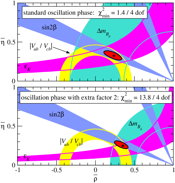
Figure 1: Unitarity triangle fit with $\Delta m_{K}$ and $\Delta m_{B_{d}}$ obtained from the standard oscillation phase (upper panel) and the oscillation phase with the extra factor of two (lower panel). The shaded regions correspond to the 95% CL regions (2 dof) obtained from the constraints given by $\varepsilon_{K},|V_{ub}/V_{cb}|,\Delta m_{B_{d}}$ and $\sin 2\beta$. In addition, constraints from the measurement of the angles $\alpha$ and $\gamma$ are used in the fit (not shown in the figure). The ellipses correspond to the 95% CL regions from all data combined, and the stars mark the best fit points.

Let us now discuss how an extra factor of two in the oscillation phase will affect the UT fit. If such a factor is present the mass differences inferred from particle–antiparticle oscillation experiments will be two times smaller. Therefore, whenever in the UT analysis a mass difference inferred from oscillations enters one has to use

$$\overline{\Delta m}=r\,\Delta m$$ (28)

with $r=1/2$, where $\Delta m$ is the value obtained with the standard oscillation phase, i.e. this is the value which is given by the Particle Data Group [48]. In the lower panel of Fig. 1 we show the result of the UT fit by using the extra factor of two in the oscillation phase. This factor affects two observables relevant for the UT fit.

1. In the prediction for $\varepsilon_{K}$ shown in Eq. (24) the experimental value for $\Delta m_{K}$ is used. Since this value is obtained from $K^{0}\leftrightarrows\bar{K}^{0}$ oscillations, $\Delta m_{K}$ has to be replaced by $\overline{\Delta m}_{K}$ if there is an extra factor of two in the oscillation phase. This moves the hyperbola in the ($\bar{\rho},\bar{\eta}$) plane from $\varepsilon_{K}$ to the right, as visible in Fig. 1.

2. The experimental value for $\Delta m_{B_{d}}$ given in Eq. (26) has to be replaced by $\overline{\Delta m}_{B_{d}}$, which is a factor of two smaller. Therefore, from Eq. (27) it is clear that the radius of the circle in the ($\bar{\rho},\bar{\eta}$) plane from $\Delta m_{B_{d}}$ is reduced by a factor $\sqrt{2}$, as can be seen also in Fig. 1.

The other constraints from $|V_{ub}/V_{cb}|,\sin 2\beta,\alpha$ and $\gamma$ are obtained from particle decays without involving any oscillation effect, and therefore they do not depend on the oscillation phase. One observes from Fig. 1 that the agreement of the individual constraints gets significantly worse using the extra factor of two. In particular, at 95% CL there is only a very marginal overlap of the intersection of the allowed regions from $|V_{ub}/V_{cb}|$ and $\sin 2\beta$ with the one from $\varepsilon_{K}$. The best fit point in the lower panel of Fig. 1 has $\chi^{2}_{\mathrm{min}}=13.8$, which implies a goodness of fit of only 0.8%, assuming a $\chi^{2}$-distribution for 4 dof.

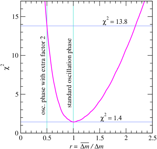
Figure 2: $\chi^{2}$ of the unitarity triangle fit as a function of the parameter $r$ defined in Eq. (28). For fixed $r$ the $\chi^{2}$ is minimized with respect to $\bar{\rho}$ and $\bar{\eta}$.

In Fig. 2 we show the $\chi^{2}$ minimized with respect to $\bar{\rho}$ and $\bar{\eta}$ as a function of the parameter $r$ given in Eq. (28). Hence, $r=1$ corresponds to the standard oscillation phase, and $r=1/2$ corresponds to the extra factor of two. From this figure one observes the remarkable feature that the best fit point occurs exactly at $r=1$. In other words, even if the extra factor in the oscillation phase is treated as a free parameter to be determined by the fit, the data prefer the standard oscillation phase. For the value $r=1/2$ we obtain a $\Delta\chi^{2}=12.4$ with respect to the best fit point, which corresponds to an exclusion at $3.5\sigma$ for 1 dof. We conclude that the extra factor of two in the oscillation phase is strongly disfavoured by the UT fit.

4.3 Robustness of the UT analysis

In this subsection we investigate the robustness of our conclusion with respect to variations of the input data for the UT fit. To this aim we show in Tab. 1 the results of our analysis by changing some of the numbers entering the UT fit. The line “standard analysis” in the table corresponds to the analysis described in the previous two subsections. In particular, exactly the input data given in Tab. 1 of Ref. [43] are used.

First we have investigated how our analysis depends on the value for $|V_{ub}|$. We show the results of the fit by using only the value from exclusive ($|V_{ub}|_{\mathrm{(excl)}}$) or inclusive ($|V_{ub}|_{\mathrm{(incl)}}$) decays, where the numbers are taken from Ref. [43]. Note that in our standard analysis both values are taken into account, as described in Appendix A. We observe from the numbers given in Tab. 1 that for the relatively small value for $|V_{ub}|$ from exclusive measurements the fit gets notably worse for $r=1/2$. In contrast, for the relatively large value from inclusive measurements the fit gets worse for the standard oscillation phase ($\chi^{2}_{\mathrm{min}}=3.9$), whereas for $r=1/2$ the fit improves with respect to the standard analysis ($\chi^{2}_{\mathrm{min}}=7.8$). The reason is that for large values of $|V_{ub}|$ the radius of the circle in the ($\bar{\rho},\bar{\eta}$) plane from $|V_{ub}/V_{cb}|$ becomes larger, which worsens the fit for $r=1$, whereas for $r=1/2$ the agreement of the individual allowed regions becomes better. Note however, that even for $|V_{ub}|_{\mathrm{(incl)}}$ the goodness of fit for $r=1/2$ is only 1%, and $r=1/2$ is disfavoured with respect to $r=1$ by 2$\sigma$. We have also performed the analysis by using the (inclusive and exclusive) averaged value $|V_{ub}|_{\mathrm{(PDG)}}$ obtained by the PDG [48]. The fit using the extra factor of two is slightly improved with respect to our standard analysis, however $r=1/2$ can still be excluded at $3.2\sigma$.

	$\chi^{2}_{\mathrm{min}}(r=1)$	$\chi^{2}_{\mathrm{min}}(r=1/2)$	number of $\sigma$
standard analysis	1.4	13.8	3.5
$|V_{ub}|_{\mathrm{(excl)}}=(33.0\pm 2.4\pm 4.6)\times 10^{-4}$	2.9	17.6	3.8
$|V_{ub}|_{\mathrm{(incl)}}=(47.0\pm 4.4)\times 10^{-4}$	3.9	7.8	2.0
$|V_{ub}|_{\mathrm{(PDG)}}=(36.7\pm 4.7)\times 10^{-4}$	1.6	11.9	3.2
$m_{c}=(1.2\pm 0.2)$ GeV	1.4	11.9	3.2
constraints on $\alpha,\gamma$ not used	0.13	9.6	3.1

Table 1: The $\chi^{2}_{\mathrm{min}}$ for the standard oscillation phase ($r=1$) and for the oscillation phase with the extra factor of two ($r=1/2$) for variations of the input data (see text for details). The column “number of $\sigma$” gives the number of standard deviations with which $r=1/2$ is disfavoured with respect to $r=1$.

Furthermore we have investigated how our result depends on the input value for the charm quark mass $m_{c}$. The value $m_{c}=(1.2\pm 0.2)$ GeV is adopted by the CKM-fitter group [36], in contrast to the value $m_{c}=(1.3\pm 0.1)$ GeV from the UTfit Collaboration [43] used in our standard analysis. The mild improvement of the fit for $r=1/2$ comes mainly from the larger error on $m_{c}$, which leads to a slightly larger allowed region from $\varepsilon_{K}$.

In the last line of Tab. 1 we have removed the constraints for the angles $\alpha$ and $\gamma$ from the fit, i.e. we use only $\varepsilon_{K},|V_{ub}/V_{cb}|,\Delta m_{B_{d}},\sin 2\beta$. We observe that the direct constraints of $\alpha$ and $\gamma$ contribute $4.2$ units of $\chi^{2}$ to the $\chi^{2}_{\mathrm{min}}$ for $r=1/2$. However, also without the constraints for $\alpha$ and $\gamma$ the extra factor of two in the oscillation phase is excluded by more than $3\sigma$.

Finally let us comment on the the very small value of $\chi^{2}_{\mathrm{min}}=0.13$ (for 2 dof), which we obtain without the constraints on $\alpha$ and $\gamma$ for the standard oscillation phase. In fact, the $\chi^{2}$-minimum value of 1.4 in the standard analysis comes mainly from $\alpha$. To include the information on this angle we are using the likelihood function from Fig. 10 of Ref. [43] (see Appendix A), which has two maxima around $107^{\circ}$ and $176^{\circ}$. The maximum at $176^{\circ}$ is slightly preferred, whereas the UT fit requires the other maximum. The very small $\chi^{2}$-minimum value obtained without using the likelihood for $\alpha$ shows that the fit is dominated by rather large theoretical errors. Therefore, $\chi^{2}$ is significantly lower as expected just from statistics. The fact that even with these assumptions on theoretical errors the $\chi^{2}$ is large for $r=1/2$ implies that the exclusion of the extra factor of two in the oscillation phase is rather robust.

5 Conclusions

In this paper we have reconsidered claims that the standard oscillation phase (19) has to be corrected by extra factors. We have focused on possible tests of these extra factors by using experimental data. The usual starting point to derive these non-quantum-theoretical expressions for the oscillation phase is Eq. (11), which says that mass eigenstates with different masses need different times to reach the spatial point where the interference of the amplitudes for the different mass eigenstates takes place. In this way we have derived the phase $\overline{\Delta\varphi}$ of Eq. (14). The aim of our theoretical discussion was to consider both neutrino oscillations and oscillations of neutral flavoured mesons. For $M^{0}-\bar{M}^{0}$ oscillations, it was important to include the non-relativistic limit in our phase considerations.

We have obtained the following results:

1. The non-quantum-theoretical phase $\overline{\Delta\varphi}$ of Eq. (14) becomes ambiguous in the non-relativistic case, because it contains a small but arbitrary momentum difference $\Delta p$. We have stressed that in the correct quantum-theoretical treatment, where the amplitudes interfere at the same time, this arbitrary term does not show up.

2. If we adjust $\Delta p$ in Eq. (14) such that the mass eigenstates have the same energy, then a momentum-dependent extra factor appears in $\overline{\Delta\varphi}$—see Eq. (17). We have shown that this extra momentum dependence is in disagreement with measurements of the $K_{L}-K_{S}$ mass difference at different kaon energies.

3. If $\Delta p=0$, the notorious factor of two appears in $\overline{\Delta\varphi}$—see Eq. (16). We have demonstrated that using $K_{L}-K_{S}$ and $B_{dH}-B_{dL}$ mass differences extracted from the data with the extra factor of two in the $K^{0}\leftrightarrows\bar{K}^{0}$ and $B_{d}^{0}\leftrightarrows\bar{B}_{d}^{0}$ oscillation phases, respectively, the unitarity triangle fit in the Standard Model becomes significantly worse compared to the fit with the standard mass differences. The phase with the extra factor of two is excluded at more than three standard deviations with respect to the standard phase.

Concerning this last point, as an additional check, we have treated the extra factor in the oscillation phase as a free parameter $r$ (see Eq. (28)) and considered $\chi^{2}$ as a function of $r$. It is remarkable that the minimum of $\chi^{2}$ occurs nearly precisely at $r=1$, which corresponds to the standard oscillation phase. This result can be regarded as a successful test of quantum theory. It is likely that in the future, with accumulated data used in the unitarity triangle fit, the exclusion of the extra factor of two will become even more significant.

Acknowledgements: S.M.B. acknowledges the support by the Italian Program “Rientro dei Cervelli”. W.G. would like to thank S.T. Petcov for an invitation to SISSA, where part of this work was performed. He is also grateful to A.Yu. Smirnov for a useful discussion. T.S. is supported by a “Marie Curie Intra-European Fellowship within the 6th European Community Framework Programme.”

Appendix A Details of our UT fit procedure

The fit of the UT is performed by adopting the following $\chi^{2}$-function:

$$\chi^{2}(\bar{\rho},\bar{\eta},\hat{B}_{K},|V_{ub}|) = \sum_{i,j}(x_{i}^{\mathrm{exp}}-x_{i}^{\mathrm{pred}})S^{-1}_{ij}(x_{j}^{\mathrm{exp}}-x_{j}^{\mathrm{pred}})+\chi^{2}_{\alpha}$$ (29)

$$+ \chi^{2}_{\mathrm{syst}}(\hat{B}_{K})+\chi^{2}_{\mathrm{syst}}(|V_{ub}|)$$

The final $\chi^{2}$ is obtained by minimizing Eq. (29) with respect to $\hat{B}_{K}$ and $|V_{ub}|$:

$$\chi^{2}(\bar{\rho},\bar{\eta})=\mathrm{Min}\left[\chi^{2}(\bar{\rho},\bar{\eta},\hat{B}_{K},|V_{ub}|);\,\hat{B}_{K},|V_{ub}|\right]\,.$$ (30)

In Eq. (29) the indices $i,j$ run over $(\varepsilon_{K},|V_{ub}/V_{cb}|,\Delta m_{B_{d}},\beta,\gamma)$ and $S_{ij}$ is the covariance matrix of these observables containing the experimental as well as theoretical uncertainties. It also takes into account correlations between the various observables induced by the experimental errors of parameters such as $m_{t},\lambda$ and $|V_{cb}|$, which are common to more than one observable. The term $\chi^{2}_{\alpha}$ contains the information on the angle $\alpha$, and is defined as $\chi^{2}_{\alpha}=-2\ln[\mathcal{L}(\alpha)/\mathrm{Max}\,\mathcal{L}(\alpha)]$, where $\mathcal{L}(\alpha)$ is the likelihood function for $\alpha$ read off from Fig. 10 of Ref. [43].

For the treatment of theoretical uncertainties we follow the common practice in UT fits to split the error into a Gaussian part and into a “flat” part, which cannot be assigned a probabilistic interpretation [36, 42, 43]. For the parameter $\hat{B}_{K}$ relevant for $\varepsilon_{K}$ one has $\hat{B}_{K}=0.86\pm 0.06\pm 0.14$, where the first error is Gaussian and the second is “flat”. To include both errors in our fit we construct a likelihood function $\mathcal{L}(\hat{B}_{k})$ by convoluting a Gaussian distribution with width $0.06$ with a flat distribution which is non-zero in the interval $[-0.14,+0.14]$ and zero outside. Then this likelihood is converted into a $\chi^{2}$ by $\chi^{2}_{\mathrm{syst}}(\hat{B}_{K})=-2\ln[\mathcal{L}(\hat{B}_{k})/\mathrm{Max}\mathcal{L}(\hat{B}_{k})]$ which is added to the total $\chi^{2}$ according to Eq. (29). The resulting $\chi^{2}$ is minimised for fixed $\bar{\rho}$ and $\bar{\eta}$ with respect to $\hat{B}_{K}$.

The value of $|V_{ub}|$ can be obtained from exclusive and inclusive decays, where the exclusive measurement suffers from theoretical uncertainties characterized by a “flat” error (see e.g. Tab. 1 of Ref. [43]). In our standard analysis we include both values by constructing a likelihood function $\mathcal{L}(|V_{ub}|)=\mathcal{L}_{\mathrm{excl}}(|V_{ub}|)\times\mathcal{L}_{\mathrm{incl}}(|V_{ub}|)$, where $\mathcal{L}_{\mathrm{excl}}(|V_{ub}|)$ is obtained similar as in the case of $\hat{B}_{K}$ by folding a Gaussian and a flat distribution, whereas $\mathcal{L}_{\mathrm{incl}}(|V_{ub}|)$ is just a Gaussian distribution. Finally, the term $\chi^{2}_{\mathrm{syst}}(|V_{ub}|)$ in Eq. (29) is obtained by $\chi^{2}_{\mathrm{syst}}(|V_{ub}|)=-2\ln[\mathcal{L}(|V_{ub}|)/\mathrm{Max}\mathcal{L}(|V_{ub}|)]$. The dependence of our results on the treatment of $|V_{ub}|$ is discussed in Sec. 4.3.

References

- [1] Super-Kamiokande Collaboration, Y. Fukuda et al., Phys. Rev. Lett. 81 (1998) 1562 [hep-ex/9807003].
- [2] Super-Kamiokande Collaboration, S. Fukuda et al., Phys. Lett. B 539 (2002) 179 [hep-ex/0205075].
- [3] SNO Collaboration, S.N. Ahmed et al., Phys. Rev. Lett. 92 (2004) 181301 [nucl-ex/0309004].
- [4] KamLAND Collaboration, T. Araki et al., hep-ex/0406035.
- [5] K2K Collaboration, M.H. Ahn et al., Phys. Rev. Lett. 90 (2003) 041801 [hep-ex/0212007].
- [6] M. Maltoni, T. Schwetz, M. Tórtola, J.W.F. Valle, New. J. Phys. 6 (2004) 122, focus issue on neutrino physics edited by F. Halzen, M. Lindner, A. Suzuki [hep-ph/0405172].
- [7] LSND Collaboration, A. Aguilar et al., Phys. Rev. D 64 (2001) 112007 [hep-ex/0104049].
- [8] MiniBooNE Collaboration, T. Hart (for the collaboration), AIP Conf. Proc. 698 (2004) 270.
- [9] Super-Kamiokande Collaboration, Y. Ashie et al., Phys. Rev. Lett. 93 (2004) 101801 [hep-ex/0404034].
-
[10]
S.M. Bilenky, C. Giunti, and W. Grimus,
Prog. Part. Nucl. Phys. 43 (1999) 1 [hep-ph/9812360];
M.C. Gonzalez-Garcia and Y. Nir, Rev. Mod. Phys. 75 (2003) 345 [hep-ph/0202058];
S. Pakvasa and J.W.F. Valle, Proc. Indian National Acad. Sci. 70A (2003) 189 [hep-ph/0301061];
W. Grimus, in Lectures on Flavor Physics, edited by U.-G. Meißner, W. Plessas (Springer-Verlag, New York 2004), p. 169 [hep-ph/0307149];
V. Barger, D. Marfatia, and K. Whisnant, Int. J. Mod. Phys. E 12 (2003) 569 [hep-ph/0308123];
A.Yu. Smirnov, Int. J. Mod. Phys. A 19 (2004) 1180 [hep-ph/0311259]. - [11] V. Gribov, B. Pontecorvo, Phys. Lett. 28B (1969) 493.
-
[12]
S.M. Bilenky, B. Pontecorvo, Lett. Nuovo Cim. 17 (1976) 569;
S.M. Bilenky, B. Pontecorvo, Phys. Rep. 41 (1978) 225. - [13] H. Fritzsch, P. Minkowski, Phys. Lett. 62B (1976) 72.
-
[14]
S.M. Bilenky, hep-ph/9908335;
S.M. Bilenky, report at the Nobel Symposium on Neutrino Physics, Haga Slott, Enkoping, Sweden, August 19–24, 2004, hep-ph/0410090. - [15] B. Kayser, Phys. Rev. D 24 (1981) 110.
-
[16]
I.Yu. Kobzarev, B.V. Martemyanov, L.B. Okun, M.G. Schepkin,
Sov. J. Nucl. Phys. 35 (1982) 708;
A.D. Dolgov, L.B. Okun, M.V. Rotaev, M.G. Schepkin, hep-ph/0407189. - [17] K. Kiers, S. Nussinov, N. Weiss, Phys. Rev. D 53 (1996) 537 [hep-ph/9506271].
- [18] C. Giunti, C.W. Kim, J.A. Lee, Phys. Rev. D 48 (1993) 4310 [hep-ph/9305276].
- [19] J. Rich, Phys. Rev. D 48 (1993) 4318.
-
[20]
W. Grimus, P. Stockinger,
Phys. Rev. D 54 (1996) 3414 [hep-ph/9603430];
W. Grimus, P. Stockinger, S. Mohanty, Phys. Rev. D 59 (1999) 013011 [hep-ph/9807442]. - [21] L. Stodolsky, Phys. Rev. D 58 (1998) 036006 [hep-ph/9802387].
- [22] C.Y. Cardall, Phys. Rev. D 61 (2000) 073006 [hep-ph/9909332].
- [23] C. Giunti, C.W. Kim, Found. Phys. Lett. 14 (2001) 213 [hep-ph/0011074].
- [24] M. Beuthe, Phys. Rev. D 66 (2002) 013003 [hep-ph/0202068].
- [25] H.J. Lipkin, Phys. Lett. B 579 (2004) 355 [hep-ph/0304187].
- [26] M. Zrałek, Acta Phys. Pol. B 29 (1998) 3925 [hep-ph/9810543].
- [27] S.M. Bilenky, C. Giunti, Int. J. Mod. Phys. A 16 (2001) 3931 [hep-ph/0102320].
- [28] M. Beuthe, Phys. Repts. 375 (2003) 105 [hep-ph/0109119].
- [29] C. Giunti, hep-ph/0409230.
- [30] J.H. Field, Eur. Phys. J. C 30 (2003) 305 [hep-ph/0211199].
-
[31]
S. De Leo, G. Ducati, P. Rotelli,
Mod. Phys. Lett. A 15 (2000) 2057 [hep-ph/9906460];
S. De Leo, C.C. Nishi, P. Rotelli, Int. J. Mod. Phys. A 19 (2004) 677 [hep-ph/0208086]. - [32] L.B. Okun, M.G. Schepkin, I.S. Tsukerman, Nucl. Phys. B 650 (2003) 443 (Err. ibid. B 656 (2003) 255) [hep-ph/0211241].
- [33] H.J. Lipkin, Phys. Lett. B 348 (1995) 604 [hep-ph/9501269].
- [34] Y.N. Srivastava, A. Widom, E. Sassaroli, Phys. Lett. B 344 (1995) 436.
- [35] B. Ancochea, A. Bramon, R. Muñoz-Tapia, M. Nowakowski, Phys. Lett. B 389 (1996) 149 [hep-ph/9605454].
- [36] J. Charles et al., hep-ph/0406184.
- [37] BaBar Collaboration, B. Aubert et al., Phys. Lett. 89 (2002) 201802.
- [38] Belle Collaboration, K. Abe et al., hep-ex/0408111.
- [39] A.J. Buras, in Proceedings of the International School of Subnuclear Physics, Erice, August 27 – September 5, 2000, edited by A. Zichichi (World Scientific, Singapore 2001), p. 200 [hep-ph/0101336].
- [40] A.J. Buras, in Lectures on Flavor Physics, edited by U.-G. Meißner, W. Plessas (Springer-Verlag, New York 2004), p. 169 [hep-ph/0307203].
- [41] J.P. Silva, hep-ph/0410351.
- [42] M. Ciuchini et al., JHEP 0107 (2001) 013 [hep-ph/0012308].
- [43] M. Bona et al., hep-ph/0501199.
- [44] J.H. Christenson, J.H. Goldman, E. Hummel, S.D. Roth, T.W.L. Sanford, J. Sculli, Phys. Rev. Lett. 43 (1979) 1209.
- [45] A. Angelopoulos et al., CPLEAR Collaboration, Phys. Lett. B 444 (1998) 38.
- [46] A. Alavi-Harati et al., KTeV Collaboration, Phys. Rev. D 67 (2003) 012005 (Err. ibid. D 70 (2004) 079904) [hep-ex/0208007].
- [47] A.Yu. Smirnov, hep-ph/0306075.
- [48] Particle Data Group, S. Eidelman et al., Phys. Lett. B 592 (2004) 1.