Two-loop scalar self-energies and pole masses in a general
renormalizable theory with massless gauge bosons

Abstract

I present the two-loop self-energy functions for scalar bosons in a general renormalizable theory, within the approximation that vector bosons are treated as massless or equivalently that gauge symmetries are unbroken. This enables the computation of the two-loop physical pole masses of scalar particles in that approximation. The calculations are done simultaneously in the mass-independent $\overline{\rm MS}$, $\overline{\rm DR}$, and $\overline{\rm DR}^{\prime}$ renormalization schemes, and with arbitrary covariant gauge fixing. As an example, I present the two-loop SUSYQCD corrections to squark masses, which can increase the known one-loop results by of order one percent. More generally, it is now straightforward to implement all two-loop sfermion pole mass computations in supersymmetry using the results given here, neglecting only the electroweak vector boson masses compared to the superpartner masses in the two-loop parts.

I Introduction

Low-energy supersymmetry provides a way of understanding the small ratio of the electroweak breaking scale in the Standard Model to other very high energy scales. This requires the existence of complex scalar superpartners for each of the known quarks and leptons, with masses not far above 1 TeV. These squarks and sleptons should be accessible to the Fermilab Tevatron $p\overline{p}$ collider or the CERN Large Hadron Collider, and their masses can be measured with refined precision at a future linear $e^{+}e^{-}$ collider; see for example LHCILC and references therein. The match between these measurements and particular models of supersymmetry breaking will then require calculations at the two-loop level of precision, at least. An important part of this is the calculation of self-energy functions, which can in turn be used to calculate the physical masses of the new particles.

In general, the mass given by the position of the complex pole in the propagator is a gauge-invariant and renormalization scale-invariant quantity Tarrach:1980up -Gambino:1999ai . The pole mass does suffer from ambiguities poleambiguities due to infrared physics associated with the QCD confinement scale, but these are probably not large enough to cause a practical problem for strongly-interacting superpartners. The pole mass should be closely related in a calculable way to the kinematic observable mass reported by experiments massdefs . In recent years, many important higher-order calculations of self-energy functions and pole masses in the Standard Model have been performed, including two-loop Gray:1990yh -Jegerlehner:2003py and three-loop Chetyrkin:1999qi -Melnikov:2000qh contributions for quarks, and two-loop results for electroweak vector bosons Chang:1981qq -Jegerlehner:2001fb , as well as two-loop results for top and bottom quarks in supersymmetry quarkpoleSUSY .

In a previous paper Martin:2003it , I provided partial results for the two-loop self-energy functions for scalars in a general renormalizable theory, using the approximation that no more than one vector boson propagator is included. That is a useful approximation for the Higgs scalar boson(s), for which the most important contributions at the two-loop level involve the strong interactions and/or Yukawa couplings. In this paper, I will extend the previous result by including the contributions for any number of vector boson lines, within the approximation that the gauge symmetry is unbroken so that the vector bosons are massless. Because of the experimental exclusions of light sfermions already achieved by the CERN LEP $e^{+}e^{-}$ collider LEPSUSY and the Fermilab Tevatron $p\overline{p}$ collider squarksDzero ; squarksCDF , this will likely give a very good approximation for the squark and slepton pole masses. (Here, the effects of non-zero $W$ and $Z$ boson masses can be included as usual in the one-loop part Pierce:1996zz , and neglected in the two-loop part.)

II Notations and Setup

Let us write the tree-level squared-mass eigenstate fields of the theory as a set of real scalars $R_{i}$, two-component Weyl fermions $\psi_{I}$, and vector bosons $V^{\mu}_{A}$. Scalar field indices are $i,j,k,\ldots$, fermion flavor indices are $I,J,K,\ldots$, and $A,B,C,\ldots$ run over the adjoint representation of the gauge group, while $\mu,\nu,\ldots$ are space-time vector indices. Repeated indices of all types are summed over unless otherwise noted. The kinetic part of the Lagrangian is taken to be:

$${\cal L}_{\rm kin} = -\frac{1}{2}\partial_{\mu}R_{i}\partial^{\mu}R_{i}-\frac{1}{2}m^{2}_{i}R_{i}^{2}$$ (2.1)

$$-i\psi^{\dagger I}\overline{\sigma}^{\mu}\partial_{\mu}\psi_{I}-\frac{1}{2}(M^{IJ}\psi_{I}\psi_{J}+{\rm c.c.})$$

$$-\frac{1}{2}(\partial_{\mu}V_{\nu}^{A}-\partial_{\nu}V_{\mu}^{A})\partial^{\mu}V^{\nu}_{A}.$$

The metric tensor has signature ($-$$+$$+$$+$). The non-gauge interactions of these fields are given by:

$${\cal L}_{\rm int} = -\frac{1}{6}\lambda^{ijk}R_{i}R_{j}R_{k}-\frac{1}{24}\lambda^{ijkm}R_{i}R_{j}R_{k}R_{m}$$ (2.2)

$$-\frac{1}{2}(y^{JKi}\psi_{J}\psi_{K}R_{i}+{\rm c.c.}).$$

where $\lambda^{ijk}$ and $\lambda^{ijkm}$ are real couplings and the Yukawa couplings $y^{JKi}$ are symmetric complex matrices on the indices $J,K$, for each $i$. Raising or lowering of fermion indices implies complex conjugation, so

$$M_{IJ}\equiv(M^{IJ})^{*},\qquad y_{JKi}\equiv(y^{JKi})^{*}.$$ (2.3)

The heights of real scalar and vector indices have no significance, and are chosen for convenience. The scalar squared masses $m_{i}^{2}$ and the fermion squared masses $M_{IK}M^{KJ}=m^{2}_{I}\delta_{I}^{J}$ are taken to have been diagonalized (by an appropriate rotation of the fields if necessary). However, the fermion mass matrix $M^{IJ}$ is not necessarily diagonal, but must have non-zero entries only when $I$ and $J$ label two-component fermions with the same squared mass and in conjugate representations of the gauge group.

In order to completely specify the pertinent features of the gauge interactions of the theory, let $T^{A}$ be the Hermitian generator matrices of the gauge group for a (possibly reducible) representation $R$. They are labeled by an adjoint representation index $A$ corresponding to the vector bosons of the theory, $V_{A}^{\mu}$. They satisfy $[T^{A},T^{B}]=if^{ABC}T^{C}$, where $f^{ABC}$ are the totally antisymmetric structure constants of the gauge group. Then results below are written in terms of the invariants:

$${(T^{A}T^{A})_{i}}^{j} = C(i)\delta_{i}^{j},$$ (2.4)

$${\rm Tr}[T^{A}T^{B}] = I(R)\delta^{AB},$$ (2.5)

$$f^{ACD}f^{BCD} = C(G)\delta^{AB},$$ (2.6)

which define the quadratic Casimir invariant for the representation carrying the index $i$, the total Dynkin index summed over the representation $R$, and the Casimir invariant of the adjoint representation of the group, respectively. When the gauge group contains several simple or $U(1)$ factors labeled $a,b,c,\ldots$ with distinct gauge couplings $g_{a}$, the corresponding invariants are written $C_{a}(i)$, $I_{a}(R)$, and $C_{a}(G)$. The normalization is such that for $SU(N)$, $C(G)=N$ and each fundamental representation has $C(i)=(N^{2}-1)/2N$ and contributes $1/2$ to $I(R)$. For a $U(1)$ gauge group, $C(G)=0$ and a representation with charge $q$ has $C(i)=q^{2}$ and contributes $q^{2}$ to $I(R)$. The results given below will be presented in terms of these group theory invariants for the representations carried by the scalar and fermion degrees of freedom.

The computations in this paper are performed in a general gauge with a vector boson propagator obtained by covariant gauge fixing in the usual way:

$$-i\delta_{AB}[\eta^{\mu\nu}/k^{2}+(\xi-1)k^{\mu}k^{\nu}/(k^{2})^{2}].$$ (2.7)

Here $\xi=0$ for Landau gauge and $\xi=1$ for Feynman gauge and $\xi=3$ for the Fried-Yennie gauge FriedYennie , for a vector boson carrying 4-momentum $k^{\mu}$. Infrared divergences are dealt with by first computing with a finite vector boson mass, and later taking the massless vector limit. All contributions involving gauge boson loops implicitly include the corresponding contributions of ghost loops.

For each Feynman diagram, the integrations over internal momenta are regulated by continuing to $d=4-2\epsilon$ dimensions, according to

$$\int d^{4}k\rightarrow(2\pi\mu)^{2\epsilon}\int d^{d}k.$$ (2.8)

In the dimensional regularization scheme, the vector bosons also have $d$ components, while in the dimensional reduction scheme they have $d$ ordinary components and $2\epsilon$ additional components known as epsilon scalars. For the present case of massless vector bosons, this means that the 4-dimensional metric in the vector propagator of eq. (2.7) is replaced by

$$\eta^{\mu\nu}/k^{2} \rightarrow g^{\mu\nu}/k^{2}+\hat{g}^{\mu\nu}/(k^{2}+m_{\epsilon}^{2}),$$ (2.9)

where $g^{\mu\nu}$ is projected onto a formal $d$–dimensional subspace, and $\hat{g}^{\mu\nu}$ onto the complementary $2\epsilon$–dimensional subspace. Counterterms for the one-loop sub-divergences and the remaining two-loop divergences are added, according to the rules of minimal subtraction, to give finite results, which then depend on the renormalization scale $Q$ given by

$$Q^{2}=4\pi e^{-\gamma}\mu^{2}.$$ (2.10)

Logarithms of dimensionful quantities are always written in terms of

$${\overline{\rm ln}}X\equiv\ln(X/Q^{2}).$$ (2.11)

The resulting renormalization schemes are known as $\overline{\rm MS}$ MSbar and $\overline{\rm DR}$ DRbar , respectively, for the cases in which $\hat{g}^{\mu\nu}$ is not and is included.

The epsilon-scalar squared mass parameter $m_{\epsilon}^{2}$ appearing in the $\overline{\rm DR}$ scheme is unphysical. One could set $m_{\epsilon}^{2}$ equal to zero at any fixed renormalization scale, but then it will be non-zero at other renormalization scales, since it has a non-homogeneous beta function Jack:1994kd . Furthermore, under renormalization group evolution it will feed into the ordinary scalar squared masses in the $\overline{\rm DR}$ scheme. Fortunately, a redefinition (given in DRbarprime at one-loop order, and at two-loop order in effpot ) of the ordinary scalar squared masses completely removes the dependence on the unphysical epsilon scalar squared mass $m_{\epsilon}^{2}$ from the renormalization group equations and the equations relating tree-level parameters to physical observables. The resulting $\overline{\rm DR}^{\prime}$ scheme DRbarprime is therefore appropriate for softly-broken supersymmetric theories such as the Minimal Supersymmetric Standard Model (MSSM). In this paper, calculations will be presented simultaneously in all three schemes, using the following two devices. First,

$$\delta_{\overline{\rm MS}}\equiv\begin{cases}1&\text{for}\quad\overline{\rm MS}\\ 0&\text{for}\quad\overline{\rm DR},\>\overline{\rm DR}^{\prime}.\end{cases}$$ (2.12)

Second, terms that involve the unphysical parameter $m_{\epsilon}^{2}$ should be construed below to apply only to the $\overline{\rm DR}$ scheme, not the $\overline{\rm DR}^{\prime}$ or $\overline{\rm MS}$ schemes.

A main objective of this paper is to compute the two-loop scalar self-energy

$$\Pi_{ij}(s)=\frac{1}{16\pi^{2}}\Pi_{ij}^{(1)}+\frac{1}{(16\pi^{2})^{2}}\Pi_{ij}^{(2)}+\ldots,$$ (2.13)

a (complex, in general) symmetric matrix, as a function of

$$s=-p^{2},$$ (2.14)

where $p^{\mu}$ is the external momentum. Note that $s$ is taken to be real with an infinitesimal positive imaginary part to resolve the branch cuts. The self-energy function $\Pi_{ij}$ is calculated as the sum of connected, one-particle irreducible, two-point Feynman diagrams. It is gauge-dependent, but can be used to obtain a gauge-invariant physical squared mass, defined as the position of the complex pole, with non-positive imaginary part, in the propagator obtained from the perturbative Taylor expansion of the self-energy function. For scalar particles with tree-level renormalized (running) squared masses $m_{k}^{2}$, the two-loop pole squared masses

$$s_{k}=M_{k}^{2}-i\Gamma_{k}M_{k}$$ (2.15)

are obtained as the solutions to

$$\mbox{Det}\left[(m_{i}^{2}-s_{k})\delta_{ij}+\Pi_{ij}(s_{k})\right]=0.$$ (2.16)

A gauge-invariant and renormalization scale invariant solution at two-loop order is obtained by first expanding the self-energy in a Taylor series in $s$ about the tree-level squared mass, with the result for the complex pole mass:

$$s_{k} = m_{k}^{2}+\frac{1}{16\pi^{2}}\Pi^{(1)}_{kk}+\frac{1}{(16\pi^{2})^{2}}\Bigl{[}\Pi^{(2)}_{kk}+\Pi^{(1)}_{kk}\Pi^{(1)\prime}_{kk}\phantom{xxx}$$ (2.17)

$$+\sum_{j\not=k}(\Pi^{(1)}_{kj})^{2}/(m_{k}^{2}-m_{j}^{2})\Bigr{]},$$

where the prime indicates differentiation with respect to $s$, and all self-energy functions on the right-hand side are evaluated with $s\rightarrow m_{k}^{2}$. This assumes that, as is the case for example for sfermions in the MSSM, the scalars that mix with each other are not degenerate, so that the last term is a well-defined part of a perturbative expansion. If (nearly) degenerate scalars do mix, then the appropriate version of (nearly) degenerate perturbation theory should be used instead.

One can also obtain a solution iteratively, by first taking $s_{k}=m_{k}^{2}$ as the argument of the self-energy eq. (2.16), and then taking the resulting value for $s_{k}$ and substituting it in as the argument of the self-energy function, repeating the process until sufficient numerical convergence is obtained. In this case, since $s_{k}$ has a negative imaginary part on the physical sheet and the argument $s$ of the self-energy is taken to be real with a positive imaginary part, the self-energy for complex $s$ can be defined in terms of its Taylor series expansion about a point on the real $s$ axis. However, for a theory with massless gauge bosons, the terms of a given loop order in the expansion of the self-energy have branch cuts. For example, at one loop order,

$$\Pi^{(1)}_{ij}(s)=(\xi-3)g_{a}^{2}C_{a}(i)\delta_{ij}m_{i}^{2}P(s/m_{i}^{2})+\ldots$$ (2.18)

where

$$P(x)=(x-1/x)\ln(1-x-i\varepsilon),$$ (2.19)

and the ellipses refers to terms without branch cuts. This yields a result that is not perturbative in the gauge coupling, unless one takes the Fried-Yennie gauge-fixing condition $\xi=3$. So, although the pole mass is formally gauge invariant, this iterative procedure has quite poor convergence unless $\xi=3$. At least in the examples given below in section V, I find that the iterative procedure in Fried-Yennie gauge gives good agreement with eq. (2.17), the difference being formally of three-loop order in any case, and the implementation of eq. (2.17) is simpler and computationally faster. The checks of gauge invariance and renormalization scale invariance for particular examples are also obtained most straightforwardly from eq. (2.17).

The results below will be written in terms of two-loop integral basis functions, following the notation given in evaluation ; TSIL . The one-loop and two-loop integral functions are reduced using Tarasov’s algorithm Tarasov:1997kx ; Mertig:1998vk to a set of basis integrals $A(x)$, $B(x,y)$, $I(x,y,z)$, $S(x,y,z)$, $T(x,y,z)$, $U(x,y,z,u)$, and $M(x,y,z,u,v)$, corresponding to the Feynman diagram topologies shown in fig. 1. Here $x,y,z,u,v$ are squared mass arguments, and the arguments $s$ and $Q^{2}$ are not shown explicitly, because they are the same for all functions in a given equation. The name of a particle stands for its squared mass when appearing as an argument of a loop-integral function. A prime on an argument of one of these functions indicates a derivative with respect to that argument, so that $T(x,y,z)=-S(x^{\prime},y,z)=-\partial S(x,y,z)/\partial x$. Also, $I(x,y,z)=S(x,y,z)|_{s=0}$. It is often useful to define the functions $V(x,y,z,u)=-U(x,y^{\prime},z,u)$, and ${\overline{T}}(0,y,z)=\lim_{x\rightarrow 0}[T(x,y,z)+B(y,z){\overline{\rm ln}}x]$. These and $B(x,y^{\prime})$ can be reduced to combinations of other basis functions, but they arise quite often in applications in such a way that explicit reduction would needlessly complicate the expressions. The basis integrals contain counterterms that render them ultraviolet finite. The precise definitions, and the calculation of these functions and a publicly available computer code for that purpose, are described in evaluation ; TSIL .

The one-loop and two-loop Feynman diagrams in the approximation used in this paper are shown in fig. 2, labeled according to a convention described in detail in ref. Martin:2003it . The results of their evaluations are described in the next section.

Figure 1: Feynman diagram topologies for the one- and two-loop self-energy basis integrals used in this paper. The dot on the $T$ diagram means that $T(x,y,z)=-\partial S(x,y,z)/\partial x$. The precise definitions of the integral functions and methods for their evaluation are described in evaluation ; TSIL .

0.66

Figure 2: The one-loop and two-loop Feynman diagrams for scalar boson self-energies in the approximation of this paper. Dashed lines stand for scalars, solid lines for fermions, and wavy lines for massless vector bosons. Diagrams involving vector boson loops also include the corresponding ghost loop diagrams. The label for each diagram refers to a corresponding function obtained as the result of the two-loop integration. All counterterm diagrams for each diagram are included in these functions, rendering them ultraviolet finite. For each diagram with a fermion loop, fermion mass insertions (indicated by adding a bar to the corresponding subscript $F$ in the name) are to be made in all possible ways. Diagrams indicated by $(*)$ vanish identically in the $\overline{\rm MS}$ scheme, but not in the $\overline{\rm DR}$ scheme with non-zero epsilon-scalar masses. Ref. Martin:2003it explains the naming convention.

.

III Two-loop self-energy functions

I begin by reviewing the result at one-loop order. Using the notation for loop integral functions used in Martin:2003it , the one-loop self-energy function matrix for real scalars is:

$$\Pi^{(1)}_{ij} = \frac{1}{2}\lambda^{ijkk}{\rm A}_{S}(m_{k}^{2})+\frac{1}{2}\lambda^{ikn}\lambda^{jkn}{\rm B}_{SS}(m_{k}^{2},m_{n}^{2})+{\rm Re}[y^{KNi}y_{KNj}]{\rm B}_{FF}(m_{K}^{2},m_{N}^{2})$$ (3.1)

$$+{\rm Re}[y^{KNi}y^{K^{\prime}N^{\prime}j}M_{KK^{\prime}}M_{NN^{\prime}}]{\rm B}_{{\overline{F}}{\overline{F}}}(m_{K}^{2},m_{N}^{2})+\delta_{ij}g_{a}^{2}C_{a}(i)[{\rm B}_{SV}(m_{i}^{2},0)+{\rm A}_{V}(0)]$$

Here I have not written the contribution from massive vector bosons, which can of course be consistently included in the one-loop part even if it is neglected in the two-loop part as below. In ref. Martin:2003it , the results were given in the $\overline{\rm MS}$ and $\overline{\rm DR}^{\prime}$ schemes, for which ${\rm A}_{V}(0)$ vanishes. In the $\overline{\rm DR}$ scheme, for massless vector bosons, one has instead:

$${\rm A}_{V}(0)=-2m_{\epsilon}^{2}.$$ (3.2)

Going from the $\overline{\rm DR}$ scheme to the $\overline{\rm DR}^{\prime}$ scheme at one loop order just removes this term DRbarprime . Similarly, at two-loop order, the change of scheme given in effpot removes all terms that depend explicitly on the unphysical epsilon-scalar mass. The other functions, due to the first four diagrams in fig. 2, are given in terms of the basis functions by:

$${\rm A}_{S}(x) = A(x)\,\equiv\,x({\overline{\rm ln}}x-1),$$ (3.3)

$$-{\rm B}_{SS}(x,y) = \frac{1}{2}{\rm B}_{{\overline{F}}{\overline{F}}}(x,y)\,=\,B(x,y)\equiv-\int_{0}^{1}dt\,{\overline{\rm ln}}[tx+(1-t)y-t(1-t)s-i\varepsilon]$$ (3.4)

$${\rm B}_{FF}(x,y) = (x+y-s)B(x,y)-A(x)-A(y)$$ (3.5)

$${\rm B}_{SV}(x,0) = (3-\xi)(x+s)B(0,x)+(3-2\xi)A(x)+2(\xi-1)s$$ (3.6)

$$= 4s+3x-3x{\overline{\rm ln}}x+(\xi-3)(s-x)[{\overline{\rm ln}}x+(1+x/s)\ln(1-s/x-i\varepsilon)].$$ (3.7)

At two-loop order, one can write the self-energy function as a sum of contributions from diagrams with 0, 1, and 2 or more vector lines:

$$\Pi^{(2)}_{ij}=\Pi^{(2,0)}_{ij}+\Pi^{(2,1)}_{ij}+\Pi^{(2,2)}_{ij}.$$ (3.8)

First, consider $\Pi^{(2,2)}_{ij}$, the two-loop self-energy contributions from diagrams with two or more massless vector boson (or ghost) propagators. The pertinent individual diagrams shown in fig. 2 contribute with group theory factors proportional to:

$${\rm V}_{VSSSV},{\rm Y}_{VSSV}: g_{a}^{2}g_{b}^{2}C_{a}(i)C_{b}(i)$$ (3.9)

$${\rm Z}_{VSVS},{\rm U}_{VSSV},{\rm S}_{SVV}: g_{a}^{2}C_{a}(i)[g_{b}^{2}C_{b}(i)-\frac{1}{4}g_{a}^{2}C_{a}(G)]$$ (3.10)

$${\rm M}_{VSSVS}: g_{a}^{2}C_{a}(i)[g_{b}^{2}C_{b}(i)-\frac{1}{2}g_{a}^{2}C_{a}(G)]\phantom{xxxxxxxxxxx}$$ (3.11)

$${\rm V}_{SVVVV},{\rm W}_{VVVV},{\rm Y}_{SVVV},{\rm X}_{VVV},{\rm M}_{VVSSV}: g_{a}^{4}C_{a}(i)C_{a}(G)$$ (3.12)

$${\rm V}_{SVVFF},{\rm V}_{SVV{\overline{F}}{\overline{F}}},{\rm W}_{VVFF},{\rm W}_{VV{\overline{F}}{\overline{F}}}: g_{a}^{4}C_{a}(i)I_{a}(R_{\rm fermions})$$ (3.13)

$${\rm V}_{SVVSS},{\rm W}_{VVSS},{\rm Y}_{SVVS},{\rm X}_{VVS}: g_{a}^{4}C_{a}(i)I_{a}(R_{\rm scalars}).$$ (3.14)

Reorganizing the contributions in terms of the four independent group theory factors, and writing them in terms of the basis functions, I obtain:

$$\Pi^{(2,2)}_{ij} = \delta_{ij}g_{a}^{2}C_{a}(i)\Bigl{[}g_{b}^{2}C_{b}(i)F_{1}(m^{2}_{i})+g_{a}^{2}C_{a}(G)F_{2}(m^{2}_{i})+g_{a}^{2}I_{a}(K)F_{3}(m^{2}_{i},m_{K}^{2})+g_{a}^{2}I_{a}(k)F_{4}(m^{2}_{i},m_{k}^{2})\Bigr{]}\phantom{xxx}$$ (3.15)

with loop integral functions defined by:

$$F_{1}(x)\>=\>-(3x+s)^{2}M(0,x,x,0,x)-(12x+4s)U(x,0,x,x)+8xU(x,0,0,0)+(2s-6x)T(x,0,0)$$

$$\qquad\>\>-3S(x,x,x)+[(3x+s)B(0,x)+4s-12x+(6+2s/x)A(x)]B(0,x)+7A(x)^{2}/x$$

$$\qquad\>\>-19A(x)+10x+15s/2+4[4x-3A(x)](x/s)\ln(1-s/x)$$

$$\qquad\>\>+(1-\xi)\Bigl{\{}-8xU(x,0,0,0)+4(s+x)T(x,0,0)+4[xB(0,x)+(1+s/x)A(x)+3x+s]B(0,x)$$

$$\qquad\>\>+A(x)^{2}/x-5A(x)+22x+2s+2[4x-3A(x)](x/s)\ln(1-s/x)\Bigr{\}}$$

$$\qquad\>\>+(1-\xi)^{2}\Bigl{\{}-2xU(x,0,0,0)+(s+x)T(x,0,0)+[xB(0,x)+(1+s/x)A(x)+4x+2s]B(0,x)$$

$$\qquad\>\>+A(x)^{2}/x+2A(x)+5x/2-3s/2\Bigr{\}}+\delta_{\overline{\rm MS}}[s-2x+4A(x)]$$

$$\qquad\>\>+m^{2}_{\epsilon}\Bigl{[}2A(x)/x-2-(8x/s)\ln(1-s/x)+(1-\xi)\{-2A(x)/x-6-(4x/s)\ln(1-s/x)\}\Bigr{]}$$ (3.16)

$$F_{2}(x)\>=\>[(3x+s)^{2}/2]M(0,x,x,0,x)+(s-x)^{2}M(0,0,x,x,0)+(6x+2s)U(x,0,x,x)+10xU(x,0,0,0)$$

$$\qquad\>\>+(6s-10x)T(x,0,0)+(3/2)S(x,x,x)+(13s/2-x/2)B(0,x)^{2}$$

$$\qquad\>\>+[7s/3-77x/3+6(1+s/x)A(x)]B(0,x)+6A(x)^{2}/x-47A(x)/3-10x+49s/4$$

$$\qquad\>\>+(1-\xi)\Bigl{\{}[(s-x)^{2}/2]M(0,0,x,x,0)+(s/2-11x/2)T(x,0,0)+5xU(x,0,0,0)$$

$$\qquad\>\>+[(3s-x)B(0,x)+(3+s/x)A(x)-5s-29x]B(0,x)/2+A(x)^{2}/x-7A(x)-8x+4s\Bigr{\}}$$

$$\qquad\>\>+(1-\xi)^{2}\Bigl{\{}xT(x,0,0)-(s/2+x/2)U(x,0,0,0)+[9x/4+5s/4]B(0,x)+3A(x)/2+5x/8-s/8\Bigr{\}}$$

$$\qquad\>\>+\delta_{\overline{\rm MS}}[(s+x)B(0,x)+x/2]-10m_{\epsilon}^{2}$$ (3.17)

$$F_{3}(x,y)\>=\>\{-4x[(s-x)^{2}+16(s+x)y-24y^{2}]/15y(s-x)\}T(x,y,y)$$

$$\qquad\qquad+\{[22s^{3}-14s^{2}x-38sx^{2}+30x^{3}-120s^{2}y+48sxy+8x^{2}y+128sy^{2}-64xy^{2}]/15(s-x)^{2}\}T(y,y,x)$$

$$\qquad\qquad+\{[12s^{2}x-4s^{3}-12sx^{2}+4x^{3}-86s^{2}y+44sxy+42x^{2}y+128sy^{2}-64xy^{2}]/15y(s-x)^{2}\}S(x,y,y)$$

$$\qquad\qquad+\{2(s+x)[A(y)/y+1]+2(s-x)^{2}/15y\}B(0,x)+\Bigl{\{}[8(s-x)^{2}+32(s+x)y]A(x)A(y)$$

$$\qquad\qquad+[4sx-26s^{2}+22x^{2}+64sy-32xy]A(y)^{2}+[2s^{3}-6s^{2}x+6sx^{2}-2x^{3}+52s^{2}y-40sxy-12x^{2}y$$

$$\qquad\qquad-32sy^{2}+64xy^{2}]A(x)+[56s^{2}y-8x(s-x)^{2}+144sxy-264x^{2}y-256sy^{2}+128xy^{2}]A(y)$$

$$\qquad\qquad+5s^{4}/2-23s^{3}x/2+39s^{2}x^{2}/2-29sx^{3}/2+4x^{4}+20s^{3}y-38s^{2}xy-32sx^{2}y+50x^{3}y$$

$$\qquad\qquad-244s^{2}y^{2}+240sxy^{2}-100x^{2}y^{2}+256sy^{3}-128xy^{3}\Bigr{\}}/15y(s-x)^{2}+\delta_{\overline{\rm MS}}(-2y)+2m_{\epsilon}^{2}$$ (3.18)

$$F_{4}(x,y)\>=\>\{-x[(s-x)^{2}+56(s+x)y+96y^{2}]/15y(s-x)\}T(x,y,y)$$

$$\qquad\qquad+\{[13s^{3}-11s^{2}x-20s^{2}y-17sx^{2}-8sxy-128sy^{2}+15x^{3}+92x^{2}y+64xy^{2}]/15(s-x)^{2}\}T(y,y,x)$$

$$\qquad\qquad+\{[(x-s)^{3}-69s^{2}y+26sxy+43x^{2}y-128sy^{2}+64xy^{2}]/15y(s-x)^{2}\}S(x,y,y)$$

$$\qquad\qquad+\{(s+x)[A(y)/y+1]+(s-x)^{2}/30y\}B(0,x)+\Bigl{\{}[2(s-x)^{2}-32(s+x)y]A(x)A(y)$$

$$\qquad\qquad+[32xy-14s^{2}-44sx+58x^{2}-64sy]A(y)^{2}+[(s-x)^{3}/2+28y(s^{2}-x^{2})+32y^{2}(s-2x)]A(x)$$

$$\qquad\qquad+[4sx^{2}-2s^{2}x-2x^{3}+164s^{2}y-104sxy+4x^{2}y+256sy^{2}-128xy^{2}]A(y)+5s^{4}/8-23s^{3}x/8$$

$$\qquad\qquad+39s^{2}x^{2}/8-29sx^{3}/8+x^{4}+45s^{3}y/2-42s^{2}xy-51sx^{2}y/2+45x^{3}y+24s^{2}y^{2}-280sxy^{2}$$

$$\qquad\qquad+360x^{2}y^{2}-256sy^{3}+128xy^{3}\bigr{\}}/15y(s-x)^{2}+\delta_{\overline{\rm MS}}4A(y).$$ (3.19)

In the limit $s\rightarrow x$, the function $F_{1}$ has a logarithmic singularity of the form $\ln(1-s/x)$, and $F_{3}$ and $F_{4}$ have $1/(s-x)$ and $1/(s-x)^{2}$ singularities in individual terms. After taking into account the identities mentioned in Appendix A, one can check that $F_{2}$, $F_{3}$, and $F_{4}$ are actually finite in that limit. [Because of these same identities, which hold between the basis functions due to coincident and vanishing arguments, the representations given in eqs. (3.16)-(3.19) are not unique.] Also, the functions $F_{1}$ and $F_{2}$ are both dependent on the gauge-fixing parameter $\xi$. It is therefore useful to define, for the purpose of computing the finite and gauge-invariant pole mass, the functions:

$$\widetilde{F}_{1}(x) \equiv \lim_{s\rightarrow x}\left[F_{1}(x)+[{\rm B}_{SV}(x,0)+{\rm A}_{V}(0)]{\rm B}^{\prime}_{SV}(x,0)\right]$$ (3.20)

$$= x\Bigl{(}12\pi^{2}-16\pi^{2}\ln 2-\frac{11}{8}+24\zeta(3)-\frac{39}{2}{\overline{\rm ln}}x+\frac{15}{2}{\overline{\rm ln}}^{2}x\Bigr{)}+\delta_{\overline{\rm MS}}x(4{\overline{\rm ln}}x-5)+m^{2}_{\epsilon}(6{\overline{\rm ln}}x-4)$$

$$\widetilde{F}_{2}(x) \equiv \lim_{s\rightarrow x}F_{2}(x)$$ (3.21)

$$= x\Bigl{(}\frac{1147}{16}-\frac{10\pi^{2}}{3}+8\pi^{2}\ln 2-12\zeta(3)-\frac{409}{12}{\overline{\rm ln}}x+\frac{19}{4}{\overline{\rm ln}}^{2}x\Bigr{)}+\delta_{\overline{\rm MS}}x\left(\frac{9}{2}-2{\overline{\rm ln}}x\right)-10m^{2}_{\epsilon}$$

$$\widetilde{F}_{3}(x,y) \equiv \lim_{s\rightarrow x}F_{3}(x,y)$$ (3.22)

$$= 2(x-y^{2}/x){\rm Li}_{2}(1-x/y)+8(x-y)f(\sqrt{y/x})+y\Bigl{(}18+\frac{\pi^{2}y}{3x}-6{\overline{\rm ln}}x-6{\overline{\rm ln}}y\Bigr{)}$$

$$+x\Bigl{(}-\frac{49}{4}-\frac{\pi^{2}}{3}+\frac{19}{3}{\overline{\rm ln}}x-2{\overline{\rm ln}}x{\overline{\rm ln}}y+{\overline{\rm ln}}^{2}y\Bigr{)}+\delta_{\overline{\rm MS}}(-2y)+2m_{\epsilon}^{2}$$

$$\widetilde{F}_{4}(x,y) \equiv \lim_{s\rightarrow x}F_{4}(x,y)$$ (3.23)

$$= (x+6y+y^{2}/x){\rm Li}_{2}(1-x/y)+8(x+y)f(\sqrt{y/x})+y[-4-\pi^{2}(1+y/6x)+7\ln(x/y)+3{\overline{\rm ln}}^{2}y]$$

$$+x\Bigl{(}-\frac{75}{8}-\frac{\pi^{2}}{6}+\frac{25}{6}{\overline{\rm ln}}x-{\overline{\rm ln}}x{\overline{\rm ln}}y+\frac{1}{2}{\overline{\rm ln}}^{2}y\Bigr{)}+\delta_{\overline{\rm MS}}4y({\overline{\rm ln}}y-1)$$

where

$$f(z) = z\{{\rm Li}_{2}([1-z]/[1+z])-{\rm Li}_{2}([z-1]/[1+z])+\pi^{2}/4\}.$$ (3.24)

The reason for including the term proportional to ${\rm B}^{\prime}_{SV}(x,0)\equiv\partial{\rm B}_{SV}(x,0)/\partial s$ in the definition of $\widetilde{F}_{1}$ in eq. (3.20) is that this includes the appropriate contribution from the $\Pi^{(1)}\Pi^{(1)\prime}$ term in the formula for the pole mass, eq. (2.17), exhibiting the simultaneous cancellation of the gauge dependence and the logarithmic singularity in the limit $s\rightarrow x$ .

Some useful limits are, for $x=y$:

$$\widetilde{F}_{3}(x,x) = x\Bigl{(}\frac{23}{4}-\frac{17}{3}{\overline{\rm ln}}x-{\overline{\rm ln}}^{2}x\Bigr{)}$$ (3.25)

$$+\delta_{\overline{\rm MS}}(-2x)+2m^{2}_{\epsilon},$$

$$\widetilde{F}_{4}(x,x) = x\Bigl{(}\frac{8\pi^{2}}{3}-\frac{107}{8}+\frac{25}{6}{\overline{\rm ln}}x+\frac{5}{2}{\overline{\rm ln}}^{2}x\Bigr{)}$$ (3.26)

$$+\delta_{\overline{\rm MS}}4x({\overline{\rm ln}}x-1),$$

and for $y=0$:

$$\widetilde{F}_{3}(x,0) = x\Bigl{(}\frac{19}{3}{\overline{\rm ln}}x-{\overline{\rm ln}}^{2}x-\frac{49}{4}-\frac{2\pi^{2}}{3}\Bigr{)}+2m_{\epsilon}^{2},\phantom{xxxx}$$ (3.27)

$$\widetilde{F}_{4}(x,0) = x\Bigl{(}\frac{25}{6}{\overline{\rm ln}}x-\frac{1}{2}{\overline{\rm ln}}^{2}x-\frac{75}{8}-\frac{\pi^{2}}{3}\Bigr{)},\phantom{xxxx}$$ (3.28)

and for $x=0$:

$$\widetilde{F}_{3}(0,y) = y(4-12{\overline{\rm ln}}y)+\delta_{\overline{\rm MS}}(-2y)+2m_{\epsilon}^{2},\phantom{xxxx}$$ (3.29)

$$\widetilde{F}_{4}(0,y) = y(11+3{\overline{\rm ln}}^{2}y)+\delta_{\overline{\rm MS}}4y({\overline{\rm ln}}y-1).$$ (3.30)

Next, consider $\Pi^{(2,1)}$, the contributions from diagrams with one vector line. These were already given in sections IV.C, IV.D, IV.E and V of ref. Martin:2003it , but the results can be rewritten in a somewhat nicer form in the case of massless vector bosons:

$$\Pi^{(2,1)}_{ij} = \frac{1}{2}\lambda^{ijkk}g_{a}^{2}\Bigl{\{}C_{a}(k)G_{S}(m_{k}^{2})+C_{a}(i)G_{SSS}(m_{i}^{2},m_{j}^{2},m_{k}^{2})\Bigr{\}}$$ (3.31)

$$+\frac{1}{2}\lambda^{ikn}\lambda^{jkn}g^{2}_{a}\Bigl{\{}\frac{1}{2}[C_{a}(k)+C_{a}(n)-C_{a}(i)]G_{SS}(m_{k}^{2},m_{n}^{2})$$

$$+[C_{a}(i)-C_{a}(k)+C_{a}(n)]G_{SSSS}(m_{i}^{2},m_{j}^{2},m_{k}^{2},m_{n}^{2})\Bigr{\}}$$

$$+{\rm Re}[y^{KNi}y_{KNj}]g_{a}^{2}\Bigl{\{}\frac{1}{2}[C_{a}(K)+C_{a}(N)-C_{a}(i)]G_{FF}(m_{K}^{2},m_{N}^{2})$$

$$+[C_{a}(i)-C_{a}(K)+C_{a}(N)]G_{SSFF}(m_{i}^{2},m_{j}^{2},m_{K}^{2},m_{N}^{2})\Bigr{\}}$$

$$+{\rm Re}[y^{KNi}y^{K^{\prime}N^{\prime}j}M_{KK^{\prime}}M_{NN^{\prime}}]g_{a}^{2}\Bigl{\{}\frac{1}{2}[C_{a}(K)+C_{a}(N)-C_{a}(i)]G_{{\overline{F}}{\overline{F}}}(m_{K}^{2},m_{N}^{2})$$

$$+[C_{a}(i)-C_{a}(K)+C_{a}(N)]G_{SS{\overline{F}}{\overline{F}}}(m_{i}^{2},m_{j}^{2},m_{K}^{2},m_{N}^{2})\Bigr{\}}$$

The functions $G_{SS}$, $G_{FF}$, $G_{{\overline{F}}{\overline{F}}}$, $G_{SSSS}$, $G_{SSFF}$, $G_{SS{\overline{F}}{\overline{F}}}$, were defined in equations (5.31)-(5.36) of Martin:2003it , referring to earlier results in that paper. Also I define here:

$$G_{S}(y) = {\rm W}_{SSSV}(y,y,y,0)+{\rm X}_{SSV}(y,y,0),$$ (3.32)

$$= y(-12+11{\overline{\rm ln}}y-3{\overline{\rm ln}}^{2}y)-2m^{2}_{\epsilon}{\overline{\rm ln}}y$$ (3.33)

$$G_{SSS}(x,y,z) = {\rm Y}_{VSSS}(0,x,y,z)$$ (3.34)

$$= A(z)[(3-2\xi)A(x)+(s+x)(3-\xi)B(0,x)]/(x-y)+(x\leftrightarrow y),$$ (3.35)

in terms of functions appearing in eqs. (5.1), (5.2), (5.4), and (5.5) of ref. Martin:2003it . All of these functions were written in that paper in the $\overline{\rm MS}$ and $\overline{\rm DR}^{\prime}$ schemes in a notation consistent with eq. (2.12) of the present paper. To obtain the $\overline{\rm DR}$ scheme results, one should add $-2m_{\epsilon}^{2}{\overline{\rm ln}}x$ to eq. (5.2), and $2m_{\epsilon}^{2}B(x,y^{\prime})$ to eq. (5.3), and $-2m_{\epsilon}^{2}$ to eq. (5.17), all in ref. Martin:2003it .

The functions $G_{S}(x)$, $G_{SS}(x,y)$, $G_{FF}(x,y)$, and $G_{{\overline{F}}{\overline{F}}}(x,y)$ are each independent of the gauge-fixing parameter $\xi$. The other functions are are not. However, for the purpose of computing the two-loop pole mass, one can define the gauge-invariant functions:

$$\widetilde{G}_{SSS}(x,x,z) = \lim_{s\rightarrow x}\left[G_{SSS}(x,x,z)+{\rm A}_{S}(z){\rm B}^{\prime}_{SV}(x,0)\right],$$ (3.36)

$$\widetilde{G}_{SSSS}(x,x,y,z) = \lim_{s\rightarrow x}\left[G_{SSSS}(x,x,y,z)+{\rm B}_{SS}(y,z){\rm B}^{\prime}_{SV}(x,0)\right],$$ (3.37)

$$\widetilde{G}_{SSFF}(x,x,y,z) = \lim_{s\rightarrow x}\left[G_{SSFF}(x,x,y,z)+{\rm B}_{FF}(y,z){\rm B}^{\prime}_{SV}(x,0)\right],$$ (3.38)

$$\widetilde{G}_{SS{\overline{F}}{\overline{F}}}(x,x,y,z) = \lim_{s\rightarrow x}\left[G_{SS{\overline{F}}{\overline{F}}}(x,x,y,z)+{\rm B}_{{\overline{F}}{\overline{F}}}(y,z){\rm B}^{\prime}_{SV}(x,0)\right].$$ (3.39)

The first two arguments are taken equal in these functions, because one can consistently neglect the off-diagonal entries in the two-loop part of the self-energy when computing the two-loop pole mass. As before, the reason for including the terms involving ${\rm B}^{\prime}_{SV}(x,0)=\partial{\rm B}_{SV}(x,0)/\partial s$ is that this naturally includes the corresponding parts of the term involving $\Pi^{(1)}\Pi^{(1)\prime}$ in eq. (2.17).

The result of taking the limits in eqs. (3.36)-(3.39) is:

$$\widetilde{G}_{SSS}(x,x,z) = (4-3{\overline{\rm ln}}x)A(z)$$ (3.40)

$$\widetilde{G}_{SSSS}(x,x,y,z) = 4(x-y+z)M(0,z,x,y,z)+4U(x,0,z,z)+2U(z,y,z,x)+4{\overline{T}}(0,y,z)-4S(0,y,z)/x$$ (3.41)

$$-2yT(y,0,z)/x+(2-2z/x)T(z,0,y)+2I(x,y,z)/x+3I(x^{\prime},y,z)+z(3{\overline{\rm ln}}z-7)B(y,z^{\prime})$$

$$+2({\overline{\rm ln}}x+{\overline{\rm ln}}z-8)B(y,z)+(2y{\overline{\rm ln}}y+2z{\overline{\rm ln}}z-7x/2-4y-4z)/x$$

$$\widetilde{G}_{SS{\overline{F}}{\overline{F}}}(x,x,y,z) = -2G_{SSSS}(x,x,y,z)+6zB(y,z^{\prime})(1-{\overline{\rm ln}}z)+\delta_{\overline{\rm MS}}[-4zB(y,z^{\prime})]$$ (3.42)

$$\widetilde{G}_{SSFF}(x,x,y,z) = 4[(x-y)^{2}-z^{2}]M(0,z,y,x,z)+4(x-y-z)U(x,0,z,z)-4yU(z,y,z,x)$$ (3.43)

$$+4(x-y-z){\overline{T}}(0,y,z)+(x-2z)(x-y-z)T(z,0,y)/x+2y(y+z)T(y,0,z)/x$$

$$+(4(y+z)/x-1)S(0,y,z)+2S(x,z,z)+3(x-y-z)I(x^{\prime},y,z)$$

$$+[1-2(y+z)/x]I(x,y,z)+2(x-y-z)z(3{\overline{\rm ln}}z-5)B(y,z^{\prime})+[15y+17z-7x$$

$$-2(x+y+z){\overline{\rm ln}}x+(x-y-3z){\overline{\rm ln}}z]B(y,z)+3{\overline{\rm ln}}x(y{\overline{\rm ln}}y-y+z{\overline{\rm ln}}z-z)$$

$$-y[3+2(y+z)/x]{\overline{\rm ln}}y+z[5{\overline{\rm ln}}z-15-2(y+z)/x]{\overline{\rm ln}}z+4(y+z)^{2}/x-15x/4+11y/2+33z/2$$

$$+\delta_{\overline{\rm MS}}[(y-x-z)B(y,z)+2(x-y-z)zB(y,z^{\prime})-y{\overline{\rm ln}}y+z{\overline{\rm ln}}z-3x/4+2y+2z]$$

Finally, consider the contributions from diagrams without any gauge interactions, $\Pi^{(2,0)}_{ij}$. These were already given in sections IV.A and IV.B of ref. Martin:2003it in exactly the same notation, and so will not be repeated here. However, for the purpose of computing the pole mass, it is convenient to define:

$$\widetilde{\Pi}^{(2,0)}_{i} = \lim_{s\rightarrow m_{i}^{2}}\Bigl{[}\Pi^{(2,0)}_{ii}+\Pi^{(1)}_{ii}\Bigl{\{}\frac{1}{2}(\lambda^{ikn})^{2}{\rm B}^{\prime}_{SS}(m_{k}^{2},m_{n}^{2})+|y^{KNi}|^{2}{\rm B}_{FF}^{\prime}(m_{K}^{2},m_{N}^{2})$$ (3.44)

$$+{\rm Re}[y^{KNi}y^{K^{\prime}N^{\prime}i}M_{KK^{\prime}}M_{NN^{\prime}}]{\rm B}_{{\overline{F}}{\overline{F}}}^{\prime}(m_{K}^{2},m_{N}^{2})\Bigr{\}}\Bigr{]},\phantom{xx}$$

where the primes indicate differentiation with respect to $s$. This incorporates the rest of the terms involving $\Pi^{(1)}\Pi^{(1)\prime}$ in eq. (2.17). (The derivatives of one-loop functions with respect to $s$ are easy to obtain analytically, and are given in the present notation in ref. Martin:2003it .)

The pole mass is now obtained as:

$$M^{2}_{i} = m^{2}_{i}+\frac{1}{16\pi^{2}}\widetilde{\Pi}^{(1)}_{ii}+\frac{1}{(16\pi^{2})^{2}}\Bigl{[}\widetilde{\Pi}^{(2,0)}_{i}+\widetilde{\Pi}^{(2,1)}_{i}+\widetilde{\Pi}^{(2,2)}_{i}+\sum_{j\not=i}(\widetilde{\Pi}^{(1)}_{ij})^{2}/(m_{i}^{2}-m_{j}^{2})\Bigr{]},$$ (3.45)

with no sum on $i$ implied. Here $\widetilde{\Pi}^{(2,1)}_{i}$ is obtained from $\Pi^{(2,1)}_{ii}$ by replacing the functions $G_{SSS}$, $G_{SSFF}$ and $G_{SS{\overline{F}}{\overline{F}}}$ with $\widetilde{G}_{SSS}$, $\widetilde{G}_{SSFF}$, and $\widetilde{G}_{SS{\overline{F}}{\overline{F}}}$, and $\widetilde{\Pi}^{(2,2)}_{i}$ is obtained from $\Pi^{(2,2)}_{ii}$ by replacing the functions $F_{1,2,3,4}$ with $\widetilde{F}_{1,2,3,4}$, and

$$\widetilde{\Pi}^{(1)}_{ij}=\lim_{s\rightarrow m^{2}_{i}}\Pi^{(1)}_{ij}.$$ (3.46)

It is a nice check that the limit $s\rightarrow x$ gives a finite result for the pole mass here. Also, the independence of the pole mass with respect to the choice of gauge-fixing parameter, up to terms of three-loop order, now follows immediately from the absence of $\xi$ in eqs. (3.20)-(3.23) and (3.40)-(3.44). Note that this relies on cancellations involving the two-loop and iterated one-loop self-energy function contributions to the pole mass.

IV Two-loop SUSYQCD corrections to squark self-energies and pole masses

As an example application of the preceding results, consider the two-loop strong (SUSYQCD) contributions to the squark masses in supersymmetry. Consider an approximation in which the squark mixings respect family symmetry, but can mix left- and right-handed squarks. (This is a slight generalization of the usual assumption that only the third-family squarks have a significant mixing.) The tree-level squared-mass matrices for each squark flavor can then each be treated as $2\times 2$ matrices ${\bf m}_{\tilde{q}}^{2}$ in the gauge eigenstate basis. They are diagonalized by unitary transformations:

$$\begin{pmatrix}\tilde{q}_{L}\\ \tilde{q}_{R}\end{pmatrix}=X_{\tilde{q}}\begin{pmatrix}\tilde{q}_{1}\\ \tilde{q}_{2}\end{pmatrix},$$ (4.1)

for $q=u,d,c,s,t,b$, chosen so that

$$X_{\tilde{q}}^{-1}{\bf m}^{2}_{\tilde{q}}X_{\tilde{q}}=\begin{pmatrix}m_{\tilde{q}_{1}}^{2}&0\\ 0&m^{2}_{\tilde{q}_{2}}\end{pmatrix}.$$ (4.2)

Thus, $\tilde{q}_{1}$, $\tilde{q}_{2}$ are mass eigenstates with squared masses $m^{2}_{\tilde{q}_{1}}$, $m^{2}_{\tilde{q}_{2}}$, while $\tilde{q}_{L}$, $\tilde{q}_{R}$ are the gauge eigenstates. Unitarity of the matrix $X_{\tilde{q}}$ allows one to write

$$X_{\tilde{q}}=\begin{pmatrix}L_{\tilde{q}_{1}}&L_{\tilde{q}_{2}}\\ R_{\tilde{q}_{1}}&R_{\tilde{q}_{2}}\end{pmatrix},$$ (4.3)

where $L_{\tilde{q}_{1}}=R_{\tilde{q}_{2}}^{*}=c_{\tilde{q}}$, and $R_{\tilde{q}_{1}}=-L_{\tilde{q}_{2}}^{*}=s_{\tilde{q}}$, with

$$|c_{\tilde{q}}|^{2}+|s_{\tilde{q}}|^{2}=1.$$ (4.4)

If the off-diagonal elements of the squared mass matrix are real, then $c_{\tilde{q}}$ and $s_{\tilde{q}}$ are the cosine and sine of a squark mixing angle for each of $q=t,b$. Also, to a good approximation in most realistic models, $s_{\tilde{q}}=1$ and $c_{\tilde{q}}=0$ for $q=u,d,c,s$. For convenience, I define the following combinations:

$$P_{i}^{j} = L_{\tilde{q}_{i}}L_{\tilde{q}_{j}}^{*}-R_{\tilde{q}_{i}}R_{\tilde{q}_{j}}^{*},$$ (4.5)

$$N_{i}^{j} = L_{\tilde{q}_{i}}R_{\tilde{q}_{j}}^{*}+R_{\tilde{q}_{i}}L_{\tilde{q}_{j}}^{*},$$ (4.6)

when $\tilde{q}_{i}$ and $\tilde{q}_{j}$ are of the same flavor, and $P_{i}^{j}=N_{i}^{j}=0$ otherwise. (Here, squarks are complex scalars, so the heights of indices are significant.) Also, in the following $C_{q}=4/3$ and $C_{G}=3$ are the quadratic Casimir invariants of the fundamental and adjoint representations, and $I_{q}=1/2$ is the Dynkin index of the fundamental.

The self-energies will then likewise be $2\times 2$ matrices for each of the 6 flavors. The SUSYQCD contribution to the one-loop self-energy in the $\overline{\rm DR}^{\prime}$ scheme is:

$$\Pi^{(1)j}_{i}=g_{3}^{2}C_{q}\Bigl{[}P_{i}^{k}P_{k}^{j}{\rm A}_{S}(\tilde{q}_{k})+2\delta_{i}^{j}{\rm B}_{FF}(q,\tilde{g})-2N_{i}^{j}m_{q}m_{\tilde{g}}{\rm B}_{{\overline{F}}{\overline{F}}}(q,\tilde{g})+\delta_{i}^{j}{\rm B}_{SV}(\tilde{q}_{i},0)\Bigr{]},$$ (4.7)

where $k$ is summed over the two mass eigenstates of the same flavor as $i,j$. (The other, non-SUSYQCD, one-loop contributions can be found in ref. Pierce:1996zz .)

The contributions from two-loop SUSYQCD diagrams with no gluon propagators are:

$$\Pi^{(2,0)j}_{i} = 4g_{3}^{4}C_{q}^{2}\Bigl{[}\frac{1}{4}P_{i}^{k}P_{k}^{m}P_{m}^{n}P_{n}^{j}{\rm X}_{SSS}(\tilde{q}_{k},\tilde{q}_{n},\tilde{q}_{m})+\frac{1}{2}P_{i}^{k}P_{k}^{j}{\rm W}_{SSFF}(\tilde{q}_{k},\tilde{q}_{k},q,\tilde{g})$$ (4.8)

$$-\frac{1}{2}P_{i}^{k}N_{k}^{m}P_{m}^{j}m_{q}m_{\tilde{g}}{\rm W}_{SS{\overline{F}}{\overline{F}}}(\tilde{q}_{k},\tilde{q}_{m},q,\tilde{g})+(L_{\tilde{q}_{i}}L_{\tilde{q}_{j}}^{*}|L_{\tilde{q}_{k}}|^{2}+R_{\tilde{q}_{i}}R_{\tilde{q}_{j}}^{*}|R_{\tilde{q}_{k}}|^{2}){\rm V}_{FFFFS}(\tilde{g},q,q,\tilde{g},\tilde{q}_{k})$$

$$-\delta_{i}^{j}N_{k}^{k}m_{q}m_{\tilde{g}}{\rm V}_{FF{\overline{F}}{\overline{F}}S}(\tilde{g},q,q,\tilde{g},\tilde{q}_{k})+(L_{\tilde{q}_{i}}R_{\tilde{q}_{j}}^{*}R_{\tilde{q}_{k}}L_{\tilde{q}_{k}}^{*}+R_{\tilde{q}_{i}}L_{\tilde{q}_{j}}^{*}L_{\tilde{q}_{k}}R_{\tilde{q}_{k}}^{*})m_{\tilde{g}}^{2}{\rm V}_{{\overline{F}}FF{\overline{F}}S}(\tilde{g},q,q,\tilde{g},\tilde{q}_{k})$$

$$+(L_{\tilde{q}_{i}}L_{\tilde{q}_{j}}^{*}|R_{\tilde{q}_{k}}|^{2}+R_{\tilde{q}_{i}}R_{\tilde{q}_{j}}^{*}|L_{\tilde{q}_{k}}|^{2})m_{q}^{2}{\rm V}_{F{\overline{F}}{\overline{F}}FS}(\tilde{g},q,q,\tilde{g},\tilde{q}_{k})-N_{i}^{j}m_{q}m_{\tilde{g}}{\rm V}_{{\overline{F}}F{\overline{F}}FS}(\tilde{g},q,q,\tilde{g},\tilde{q}_{k})$$

$$+(L_{\tilde{q}_{i}}R_{\tilde{q}_{j}}^{*}L_{\tilde{q}_{k}}R_{\tilde{q}_{k}}^{*}+R_{\tilde{q}_{i}}L_{\tilde{q}_{j}}^{*}R_{\tilde{q}_{k}}L_{\tilde{q}_{k}}^{*})m_{q}^{2}m_{\tilde{g}}^{2}{\rm V}_{{\overline{F}}{\overline{F}}{\overline{F}}{\overline{F}}S}(\tilde{g},q,q,\tilde{g},\tilde{q}_{k})\Bigr{]}$$

$$+g_{3}^{4}[4C_{q}^{2}-2C_{G}C_{q}]\Bigl{[}(L_{\tilde{q}_{i}}R_{\tilde{q}_{j}}^{*}R_{\tilde{q}_{k}}L_{\tilde{q}_{k}}^{*}+R_{\tilde{q}_{i}}L_{\tilde{q}_{j}}^{*}L_{\tilde{q}_{k}}R_{\tilde{q}_{k}}^{*}){\rm M}_{FFFFS}(q,\tilde{g},\tilde{g},q,\tilde{q}_{k})$$

$$-N_{i}^{j}m_{q}m_{\tilde{g}}{\rm M}_{FF{\overline{F}}{\overline{F}}S}(q,\tilde{g},\tilde{g},q,\tilde{q}_{k})+(L_{\tilde{q}_{i}}L_{\tilde{q}_{j}}^{*}|L_{\tilde{q}_{k}}|^{2}+R_{\tilde{q}_{i}}R_{\tilde{q}_{j}}^{*}|R_{\tilde{q}_{k}}|^{2})m_{\tilde{g}}^{2}{\rm M}_{F{\overline{F}}{\overline{F}}FS}(q,\tilde{g},\tilde{g},q,\tilde{q}_{k})$$

$$-\delta_{i}^{j}N_{k}^{k}m_{q}m_{\tilde{g}}{\rm M}_{F{\overline{F}}F{\overline{F}}S}(q,\tilde{g},\tilde{g},q,\tilde{q}_{k})+(L_{\tilde{q}_{i}}L_{\tilde{q}_{j}}^{*}|R_{\tilde{q}_{k}}|^{2}+R_{\tilde{q}_{i}}R_{\tilde{q}_{j}}^{*}|L_{\tilde{q}_{k}}|^{2})m_{q}^{2}{\rm M}_{F{\overline{F}}{\overline{F}}FS}(\tilde{g},q,q,\tilde{g},\tilde{q}_{k})$$

$$+(L_{\tilde{q}_{i}}R_{\tilde{q}_{j}}^{*}L_{\tilde{q}_{k}}R_{\tilde{q}_{k}}^{*}+R_{\tilde{q}_{i}}L_{\tilde{q}_{j}}^{*}R_{\tilde{q}_{k}}L_{\tilde{q}_{k}}^{*})m_{q}^{2}m_{\tilde{g}}^{2}{\rm M}_{{\overline{F}}{\overline{F}}{\overline{F}}{\overline{F}}S}(q,\tilde{g},\tilde{g},q,\tilde{q}_{k})+\frac{1}{4}P_{i}^{k}P_{k}^{m}P_{m}^{n}P_{n}^{j}{\rm S}_{SSS}(\tilde{q}_{k},\tilde{q}_{m},\tilde{q}_{n})\Bigr{]}\phantom{xxx}$$

$$+4g_{3}^{4}C_{q}I_{q}\Bigl{[}\delta_{i}^{j}{\rm V}_{FFFFS}(q,\tilde{g},\tilde{g},q_{r},\tilde{q}_{r})+\delta_{i}^{j}m_{\tilde{g}}^{2}{\rm V}_{F{\overline{F}}{\overline{F}}FS}(q,\tilde{g},\tilde{g},q_{r},\tilde{q}_{r})-2N_{i}^{j}m_{q_{r}}m_{\tilde{g}}{\rm V}_{{\overline{F}}F{\overline{F}}FS}(q,\tilde{g},\tilde{g},q_{r},\tilde{q}_{r})$$

$$+N_{i}^{j}N_{r}^{r}m_{q}m_{q_{r}}{\rm V}_{{\overline{F}}FF{\overline{F}}S}(q,\tilde{g},\tilde{g},q_{r},\tilde{q}_{r})-2\delta_{i}^{j}N_{r}^{r}m_{q_{r}}m_{\tilde{g}}{\rm V}_{FF{\overline{F}}{\overline{F}}S}(q,\tilde{g},\tilde{g},q_{r},\tilde{q}_{r})$$

$$+N_{i}^{j}N_{r}^{r}m_{q}m_{q_{r}}m_{\tilde{g}}^{2}{\rm V}_{{\overline{F}}{\overline{F}}{\overline{F}}{\overline{F}}S}(q,\tilde{g},\tilde{g},q_{r},\tilde{q}_{r})+\frac{1}{4}P_{i}^{k}P_{k}^{j}P_{r}^{s}P_{s}^{r}{\rm S}_{SSS}(\tilde{q}_{k},\tilde{q}_{r},\tilde{q}_{s})\Bigr{]}.$$

For two-loop diagrams with one gluon propagator,

$$\Pi^{(2,1)j}_{i} = g_{3}^{4}\delta_{i}^{j}\bigl{\{}C_{q}C_{G}[G_{FF}(q,\tilde{g})+G_{SSFF}(\tilde{q}_{i},\tilde{q}_{i},q,\tilde{g})]+[2C_{q}-C_{G}]C_{q}G_{SSFF}(\tilde{q}_{i},\tilde{q}_{i},\tilde{g},q)\bigr{\}}$$ (4.9)

$$-g_{3}^{4}N_{i}^{j}m_{q}m_{\tilde{g}}\bigl{\{}C_{q}C_{G}[G_{{\overline{F}}{\overline{F}}}(q,\tilde{g})+G_{SS{\overline{F}}{\overline{F}}}(\tilde{q}_{i},\tilde{q}_{j},q,\tilde{g})]+[2C_{q}-C_{G}]C_{q}G_{SS{\overline{F}}{\overline{F}}}(\tilde{q}_{i},\tilde{q}_{j},\tilde{g},q)\bigr{\}}$$

$$+g_{3}^{4}C_{q}^{2}P_{i}^{k}P_{k}^{j}\left[G_{S}(\tilde{q}_{k})+G_{SSS}(\tilde{q}_{i},\tilde{q}_{j},\tilde{q}_{k})\right].$$

Finally, for two-loop diagrams with two or more gluon lines,

$$\Pi^{(2,2)j}_{i}=g_{3}^{4}\delta_{i}^{j}C_{q}\Bigl{[}C_{q}F_{1}(\tilde{q}_{i})+C_{G}F_{2}(\tilde{q}_{i})+C_{G}F_{3}(\tilde{q}_{i},\tilde{g})+I_{q}\sum_{r}\{F_{3}(\tilde{q}_{i},q_{r})+F_{4}(\tilde{q}_{i},\tilde{q}_{r})\}\Bigr{]}.$$ (4.10)

In eqs. (4.8)-(4.10), indices $r,s$ are used when all 12 left-handed and right-handed quarks and 12 squark mass eigenstates should be summed over. Indices $k,m,n$ are used when only the two squarks with the same flavor as the external particle states $\tilde{q}_{i},\tilde{q}_{j}$ are summed over. The quark corresponding to the external squark flavor is called $q$.

The squark pole squared mass $M^{2}_{\tilde{q}_{i}}$ can now be obtained following the discussion of the previous section; see eq. (3.45). This yields:

$$M^{2}_{\tilde{q}_{i}} = m^{2}_{\tilde{q}_{i}}+\frac{1}{16\pi^{2}}\widetilde{\Pi}^{(1)i}_{i}+\frac{1}{(16\pi^{2})^{2}}\Bigl{[}\widetilde{\Pi}^{(2,0)}_{i}+\widetilde{\Pi}^{(2,1)}_{i}+\widetilde{\Pi}^{(2,2)}_{i}+\sum_{j\not=i}\widetilde{\Pi}^{(1)j}_{i}\widetilde{\Pi}^{(1)i}_{j}/(m_{\tilde{q}_{i}}^{2}-m_{\tilde{q}_{j}}^{2})\Bigr{]},$$ (4.11)

with no sum on $i$ implied. Within the approximation specified above for sfermions in the MSSM, $j$ can actually take on only one value for a given $i$, and the sfermions that mix are always non-degenerate. Here $\widetilde{\Pi}^{(1)j}_{i}$ is obtained from $\Pi^{(1)j}_{i}$ by taking $s\rightarrow m^{2}_{\tilde{q}_{i}}$. Also, $\widetilde{\Pi}^{(2,1)}_{i}$ is obtained from $\Pi^{(2,1)i}_{i}$ by replacing the functions $G_{SSS}$, $G_{SSFF}$ and $G_{SS{\overline{F}}{\overline{F}}}$ by $\widetilde{G}_{SSS}$, $\widetilde{G}_{SSFF}$, and $\widetilde{G}_{SS{\overline{F}}{\overline{F}}}$, and $\widetilde{\Pi}^{(2,2)}_{i}$ is obtained from $\Pi^{(2,2)i}_{i}$ by replacing the functions $F_{1,2,3,4}$ by $\widetilde{F}_{1,2,3,4}$, and

$$\widetilde{\Pi}^{(2,0)}_{i}=\lim_{s\rightarrow m_{\tilde{q}_{i}}^{2}}\left[\Pi^{(2,0)i}_{i}+\widetilde{\Pi}^{(1)i}_{i}2g_{3}^{2}C_{q}\{{\rm B}_{FF}^{\prime}(q,\tilde{g})-N_{i}^{i}m_{q}m_{\tilde{g}}{\rm B}_{{\overline{F}}{\overline{F}}}^{\prime}(q,\tilde{g})\}\right].$$ (4.12)

I have checked that this result for the squark pole mass is invariant under renormalization group evolution of the parameters, up to terms of three-loop order. That check is somewhat messy when non-trivial mixing is involved, and so will not be presented here in the general case. Instead, it will be shown explicitly in two simplified special cases in the next section.

V Simple examples

V.1 Squarks without mixing

In this subsection, I consider a simple (probably non-realistic) example, to demonstrate the typical size of the two-loop contribution to the squark pole masses. As an approximation, suppose that all squarks are degenerate in mass, with therefore no mixing, and that all of the quark masses can be neglected. Then, reorganizing the results of the previous section by common group theory factor rather than number of gluon propagators, one obtains for the pole squared mass of a given squark $\tilde{q}_{i}$:

$$M^{2}_{\tilde{q}_{i}} = m^{2}_{\tilde{q}_{i}}+\frac{1}{16\pi^{2}}g_{3}^{2}C_{q}\widetilde{\Pi}^{(1)}({\tilde{q}_{i}},{\tilde{g}})$$ (5.1)

$$+\frac{1}{(16\pi^{2})^{2}}g_{3}^{4}C_{q}\Bigl{[}C_{q}\widetilde{\Pi}^{(2a)}({\tilde{q}_{i}},{\tilde{g}})+C_{G}\widetilde{\Pi}^{(2b)}({\tilde{q}_{i}},{\tilde{g}})+I_{q}\sum_{r}\widetilde{\Pi}^{(2c)}({\tilde{q}_{i}},{\tilde{g}},{\tilde{q}_{r}})\Bigr{]}+\ldots$$

where

$$\widetilde{\Pi}^{(1)}(x,y) = {\rm A}_{S}(x)+2{\rm B}_{FF}(0,y)+{\rm B}_{SV}(x,0)$$ (5.2)

$$\widetilde{\Pi}^{(2a)}(x,y) = {\rm X}_{SSS}(x,x,x)+{\rm S}_{SSS}(x,x,x)+4y{\rm M}_{F{\overline{F}}{\overline{F}}FS}(0,y,y,0,x)+4{\rm V}_{FFFFS}(y,0,0,y,x)$$ (5.3)

$$+2{\rm W}_{SSFF}(x,x,0,y)+G_{S}(x)+\widetilde{G}_{SSS}(x,x,x)+2\widetilde{G}_{SSFF}(x,x,y,0)+\widetilde{F}_{1}(x)$$

$$+2\Pi^{(1)}(x,y)\,{\rm B}^{\prime}_{FF}(0,y)$$

$$\widetilde{\Pi}^{(2b)}(x,y) = -\frac{1}{2}{\rm S}_{SSS}(x,x,x)-2y{\rm M}_{F{\overline{F}}{\overline{F}}FS}(0,y,y,0,x)+G_{FF}(0,y)+\widetilde{G}_{SSFF}(x,x,0,y)$$ (5.4)

$$-\widetilde{G}_{SSFF}(x,x,y,0)+\widetilde{F}_{2}(x)+\widetilde{F}_{3}(x,y)$$

$$\widetilde{\Pi}^{(2c)}(x,y,z) = {\rm S}_{SSS}(x,z,z)+4{\rm V}_{FFFFS}(0,y,y,0,z)+4y{\rm V}_{F{\overline{F}}{\overline{F}}FS}(0,y,y,0,z)+\widetilde{F}_{3}(x,0)+\widetilde{F}_{4}(x,z).\phantom{xxx}$$ (5.5)

All of the basis integral functions on the right-hand sides of these equations are to be evaluated at $s=x$. This example has the virtue that all of these functions can be given analytically in terms of polylogarithms, with the result (in the $\overline{\rm DR}^{\prime}$ scheme):

$$\widetilde{\Pi}^{(1)}(x,y) = 2x[1+\ln(y/x)+(1-y/x)^{2}\ln(1-x/y)]+6y-4y{\overline{\rm ln}}y$$ (5.6)

$$\widetilde{\Pi}^{(2a)}(x,y) = 8(x-y)^{2}M(0,0,x,y,0)-8(x-y)yM(0,y,y,0,x)+(24x-8y-12y^{2}/x){\rm Li}_{2}(1-x/y)$$ (5.7)

$$+(1-y/x)^{2}(2x+4y-4y^{2}/x)\ln^{2}(1-x/y)+4(1-y/x)[6x-2y+4y^{2}/x-(x+y){\overline{\rm ln}}x$$

$$+(x-y-2y^{2}/x){\overline{\rm ln}}y]\ln(1-x/y)+(14x-4y)\ln^{2}(x/y)+8[y\ln(x/y)+3x-y+y^{2}/x]{\overline{\rm ln}}y$$

$$+24(y-x){\overline{\rm ln}}x+[24\zeta(3)-6+16\pi^{2}(1-\ln 2)]x-(60+8\pi^{2}/3)y+(2\pi^{2}-12)y^{2}/x$$

$$\widetilde{\Pi}^{(2b)}(x,y) = 4(x-y)[(x+y)M(0,x,y,0,y)+yM(0,y,y,0,x)]-2(x-y)^{2}[2M(0,0,x,y,0)+M(0,0,y,y,0)]\phantom{xxx}$$ (5.8)

$$+(2x-12y+12y^{2}/x){\rm Li}_{2}(1-x/y)+8(y-x)[f(\sqrt{y/x})+(1-y/x)\ln^{2}(1-x/y)]$$

$$+[(10x-8y){\overline{\rm ln}}x+(44y-16x-30y^{2}/x){\overline{\rm ln}}y+19x-80y+61y^{2}/x]\ln(1-x/y)$$

$$+(2y-x){\overline{\rm ln}}^{2}x+(8x-4y){\overline{\rm ln}}x{\overline{\rm ln}}y+(20y-7x){\overline{\rm ln}}^{2}y-(25x+16y){\overline{\rm ln}}x+(19x-66y){\overline{\rm ln}}y$$

$$+x[21-12\zeta(3)-26\pi^{2}/3+8\pi^{2}\ln 2]+y(123+14\pi^{2}/3-2\pi^{2}y/x)$$

$$\widetilde{\Pi}^{(2c)}(x,y,z) = [(x-y)(y-z)(xy-5y^{2}+3xz+yz)/xy^{2}]\{2{\rm Li}_{2}([y-z]/[y-x])+\ln^{2}(1-x/y)\}$$ (5.9)

$$+[2(y-z)(5y-z)/x]{\rm Li}_{2}(1-y/z)+[8z-4z(x+z)/y+6xz^{2}/y^{2}]{\rm Li}_{2}(1-x/z)$$

$$+8(x+z)f(\sqrt{z/x})+[6z+2yz/x-16y^{2}/x+(4z+12yz/x-2z^{2}/x-6z^{2}/y)\ln(z/y)$$

$$+(10y^{2}/x-2y){\overline{\rm ln}}y](1-x/y)\ln(1-x/y)+\{[2z(2x/y+2z/y-3xz/y^{2})]\ln(z/x)$$

$$+(1-z/x)(10y-7x-7z+6xz/y)\}\ln(1-x/z)+(16y+4z-6xz/y)\ln(y/z)+(x-6y){\overline{\rm ln}}^{2}y$$

$$-x{\overline{\rm ln}}^{2}x+[4z+(y-z)(5y-z)/x+2z(x+z)/y-3xz^{2}/y^{2}]\ln^{2}(y/z)+(2x+26y+4z){\overline{\rm ln}}z$$

$$+(9x+8z)\ln(x/z)-7x-40y-3z+(2\pi^{2}/3)(2z(x+z)/y-x-2z-3xz^{2}/y^{2}).$$

Ref. TSIL gave analytic formulas for the master integral cases $M(0,0,x,y,0)$, $M(0,y,y,0,x)|_{s=x}$. The integral $M(0,x,y,0,y)|_{s=x}$ can be reduced using recurrence relations to results found in Fleischer:1998dw , Jegerlehner:2003py , and was given in the present notation in TSIL . Also, $M(0,0,y,y,0)$ was originally found in Broadhurst:1987ei and listed in the present notation in ref. evaluation . The function $f(z)$ is defined in eq. (3.24) of the present paper.

The renormalization group scale independence of the pole mass $M_{\tilde{q}_{i}}$ can now be checked. The requirement $dM_{\tilde{q}_{i}}^{2}/dQ=0$ amounts to:

$$-\beta^{(1)}_{m^{2}_{\tilde{q}_{i}}} = g_{3}^{2}C_{q}\,Q\frac{\partial}{\partial Q}\widetilde{\Pi}^{(1)}({\tilde{q}_{i}},{\tilde{g}})$$ (5.10)

$$-\beta^{(2)}_{m^{2}_{\tilde{q}_{i}}} = g_{3}^{4}C_{q}\,Q\frac{\partial}{\partial Q}\Bigl{[}C_{q}\widetilde{\Pi}^{(2a)}({\tilde{q}_{i}},{\tilde{g}})+C_{G}\widetilde{\Pi}^{(2b)}({\tilde{q}_{i}},{\tilde{g}})+I_{q}\sum_{r}\widetilde{\Pi}^{(2c)}({\tilde{q}_{i}},{\tilde{g}},{\tilde{q}_{r}})\Bigr{]}$$ (5.11)

$$+g_{3}^{2}C_{q}\Bigl{[}\frac{2}{g_{3}}\beta^{(1)}_{g_{3}}+2m_{\tilde{g}}\beta^{(1)}_{m_{\tilde{g}}}\frac{\partial}{\partial m^{2}_{\tilde{g}}}+\beta^{(1)}_{m_{\tilde{q}_{i}}^{2}}\frac{\partial}{\partial m^{2}_{\tilde{q}_{i}}}\Bigr{]}\widetilde{\Pi}^{(1)}({\tilde{q}_{i}},{\tilde{g}})$$

(with no sum on $i$), where

$$Q\frac{dX}{dQ}\equiv\beta_{X}=\frac{1}{16\pi^{2}}\beta^{(1)}_{X}+\frac{1}{(16\pi^{2})^{2}}\beta^{(2)}_{X}+\ldots,$$ (5.12)

are the beta functions of running parameters $X=g_{3},m_{\tilde{g}},m_{\tilde{q}_{i}}^{2}$. Equations (5.10)-(5.11) can be checked using the results

$$\beta^{(1)}_{g_{3}} = g_{3}^{3}(-3C_{G}+2N_{f}I_{q}),$$ (5.13)

$$\beta^{(2)}_{g_{3}} = g_{3}^{5}[-6C_{G}^{2}+(4C_{G}+8C_{q})N_{f}I_{q}],$$ (5.14)

$$\beta^{(1)}_{m_{\tilde{g}}} = g_{3}^{2}(-6C_{G}+4N_{f}I_{q})m_{\tilde{g}},$$ (5.15)

$$\beta^{(2)}_{m_{\tilde{g}}} = g_{3}^{4}[-24C_{G}^{2}+(16C_{G}+32C_{q})N_{f}I_{q}]m_{\tilde{g}},\phantom{xxxx}$$ (5.16)

$$\beta^{(1)}_{m_{\tilde{q}_{i}}^{2}} = -8g_{3}^{2}C_{q}m_{\tilde{g}}^{2},$$ (5.17)

$$\beta^{(2)}_{m_{\tilde{q}_{i}}^{2}} = g_{3}^{4}C_{q}\Bigl{[}(-80C_{G}+48C_{q}+48N_{f}I_{q})m_{\tilde{g}}^{2}$$ (5.18)

$$+8I_{q}\sum_{r}m_{\tilde{q}_{r}}^{2}\Bigr{]},$$

with $2N_{f}$ the number of quark/squark chiral superfields (12 in the MSSM), and

$$Q\frac{\partial}{\partial Q}\widetilde{\Pi}^{(1)}(x,y) = 8y,$$ (5.19)

$$\frac{\partial}{\partial x}\widetilde{\Pi}^{(1)}(x,y) = 2-2y/x+2\ln(y/x)$$ (5.20)

$$+2(1-y^{2}/x^{2})\ln(1-x/y),$$

$$\frac{\partial}{\partial y}\widetilde{\Pi}^{(1)}(x,y) = 4+4(y/x-1)\ln(1-x/y)$$ (5.21)

$$-4{\overline{\rm ln}}y,$$

$$Q\frac{\partial}{\partial Q}\widetilde{\Pi}^{(2a)}(x,y) = -32y-16y^{2}/x+16y\ln(y/x)$$ (5.22)

$$\!\!\!\!\!\!\!\!+16y(1-y^{2}/x^{2})\ln(1-x/y),$$

$$Q\frac{\partial}{\partial Q}\widetilde{\Pi}^{(2b)}(x,y) = 12x+164y+12x\ln(y/x)$$ (5.23)

$$\!\!\!\!\!\!\!\!+(12x-72y+60y^{2}/x)\ln(1-x/y)$$

$$\!\!\!\!\!\!\!\!-72y{\overline{\rm ln}}y,\phantom{xxx}$$

$$Q\frac{\partial}{\partial Q}\widetilde{\Pi}^{(2c)}(x,y,z) = -4x-52y-8z+4x\ln(x/y)$$ (5.24)

$$\!\!\!\!\!\!\!\!+(24y-4x-20y^{2}/x)\ln(1-x/y)\phantom{xx}$$

$$\!\!\!\!\!\!\!\!+24y{\overline{\rm ln}}y,$$

which in turn follow directly from eqs. (5.6)-(5.9), noting that the master integral basis function $M(x,y,z,u,v)$ has no explicit dependence on $Q$.

This scale independence thus holds up to terms of three-loop order. To illustrate it in practice, consider the even more special case that the gluino and all squarks have equal running masses at an input renormalization scale $Q_{0}$ given by the same value, so that $Q_{0}=m_{\tilde{g}}(Q_{0})=m_{\tilde{q}}(Q_{0})$. Figure 3 then shows the scale dependence of the squark pole mass as calculated from eqs. (5.1) and (5.6)-(5.9). To make this graph, the running parameters $g_{3}$, $m_{\tilde{g}}$, and $m_{\tilde{q}}$ are each run from the input scale $Q_{0}$ to a new scale $Q$, using their two-loop renormalization group equations (5.13)-(5.18). Here I have put in the MSSM values, namely $C_{G}=3$, $C_{q}=4/3$, $I_{q}=1/2$, and $N_{f}=6$, and taken $\alpha_{S}(Q_{0})=g_{3}^{2}(Q_{0})/4\pi=0.095$. At the scale $Q$, the pole mass is recomputed, and the quantity $M_{\tilde{q}}/m_{\tilde{q}}(Q_{0})-1$ is shown; in the ideal case of an exact calculation the resulting line would be exactly horizontal. The two-loop result has a slightly improved scale dependence, as expected, but the difference between the two-loop result and the one-loop result is actually much larger than the scale dependence of the latter. This demonstrates that the scale dependence does not give an adequate estimate of the theoretical error of the calculation.

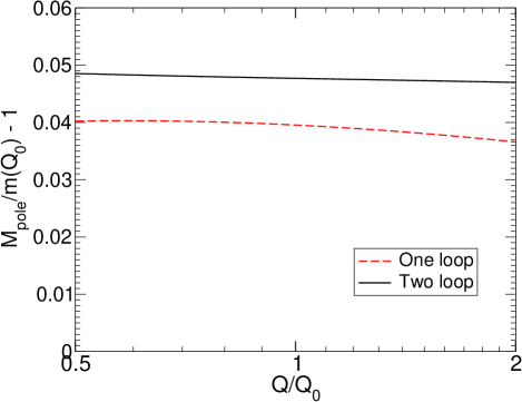
Figure 3: Dependence of the calculated pole mass for degenerate squarks on the choice of renormalization scale. The input parameters are defined by running gluino and squark masses taken to be equal at an input renormalization scale $Q_{0}=m_{\tilde{q}}(Q_{0})=m_{\tilde{g}}(Q_{0})$, with $\alpha_{S}(Q_{0})=0.095$. These parameters are then run to new scales $Q$, where the pole mass is recomputed. The vertical axis is the fractional change in the squark pole mass compared to the squark running mass at the input scale. Six squark families are assumed as in the MSSM, but quark masses, squark mixing, and non-SUSYQCD effects are neglected in this graph.

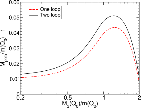
Figure 4: The SUSYQCD corrections to the squark pole mass, as in figure 3, but now as a function of the varying ratio of the tree-level running gluino mass $M_{3}(Q_{0})\equiv m_{\tilde{g}}(Q_{0})$ to the running squark masses $Q_{0}=m_{\tilde{q}}(Q_{0})$. The squark pole mass is computed at the renormalization scale $Q_{0}$.

The result at $Q=Q_{0}$ is:

$$M^{2}_{\tilde{q}} = m^{2}_{\tilde{q}}\Bigl{[}1+\frac{\alpha_{S}}{4\pi}\left(\frac{32}{3}\right)+\left(\frac{\alpha_{S}}{4\pi}\right)^{2}\Bigl{(}\frac{112}{3}$$ (5.25)

$$+\frac{664\pi^{2}}{27}+\frac{32\pi^{2}\ln 2}{9}-\frac{16\zeta(3)}{3}\Bigr{)}\Bigr{]}$$

$$= m^{2}_{\tilde{q}}\left[1+0.849\alpha_{S}+1.89\alpha_{S}^{2}\right].$$ (5.26)

There are no logarithms here, since there is only one mass scale, so the result gives some idea of the typical intrinsic size of the two-loop corrections. The one-loop correction is an increase of order 4% in the pole mass compared to the running mass evaluated at itself, while the two-loop correction adds an additional amount of order 1%.

More generally, fig. 4 shows the one-loop and two-loop corrections to the squark masses, calculated as above, but now varying the running gluino mass $M_{3}(Q_{0})\equiv m_{\tilde{g}}(Q_{0})$ at the fixed renormalization scale $Q_{0}=m_{\tilde{q}}(Q_{0})$. The two-loop part of the correction is seen to be largest when the squark masses are slightly less than the gluino mass, and does not exceed 1% over the indicated range.

In nearly all realistic models of supersymmetry breaking, $M_{3}/m_{\tilde{q}}<1.5$ at the TeV scale for the squarks of the first two families. For $M_{3}(Q_{0})$ much larger than $2m_{\tilde{q}}(Q_{0})$, there are large negative loop corrections to the squark pole mass from gluino loops. This can happen for top and bottom squarks in the MSSM, in which case the top and bottom Yukawa couplings and scalar cubic couplings must be included to give a reliable result.

V.2 Squarks in the supersymmetric limit

Let us next consider the supersymmetric limit for squarks for an $SU(n)$ supersymmetric Yang-Mills theory with gauge coupling $g$. The gaugino mass vanishes, and $N_{f}$ flavors of quarks and squarks obtain their masses solely from a superpotential

$$W=\sum_{i=1}^{N_{f}}m_{i}\overline{Q}^{i}Q_{i}.$$ (5.27)

Here, $Q_{i}$ are chiral superfields transforming in the fundamental representation, and $\overline{Q}_{i}$ in the anti-fundamental representation of the gauge group. Specializing the results of section IV to this case, I obtain two-loop squark pole squared masses:

$$M_{i}^{2}=m_{i}^{2}+\frac{1}{16\pi^{2}}\widetilde{\Pi}^{(1)}_{i}+\frac{1}{(16\pi^{2})^{2}}\widetilde{\Pi}^{(2)}_{i}$$ (5.28)

where

$$\widetilde{\Pi}^{(1)}_{i} = g^{2}C_{q}m_{i}^{2}(8-4{\overline{\rm ln}}m_{i}^{2})$$ (5.29)

$$\widetilde{\Pi}^{(2)}_{i} = g^{4}C_{q}\Bigl{(}C_{q}m_{i}^{2}\Bigl{[}40\pi^{2}/3-16\pi^{2}\ln 2$$ (5.30)

$$+24\zeta(3)-28-8{\overline{\rm ln}}m_{i}^{2}+8{\overline{\rm ln}}^{2}m_{i}^{2}\Bigr{]}$$

$$+C_{G}m_{i}^{2}\Bigl{[}66-4\pi^{2}+8\pi^{2}\ln 2-12\zeta(3)$$

$$-36{\overline{\rm ln}}m_{i}^{2}+6{\overline{\rm ln}}^{2}m_{i}^{2}\Bigr{]}$$

$$+2I_{q}\sum_{j=1}^{N_{f}}h(m_{i}^{2},m_{j}^{2})\Bigr{)},\phantom{xxxxx}$$

in which

$$h(x,y) = 4(x+y)[{\rm Li}_{2}(1-x/y)-\pi^{2}/6]$$ (5.31)

$$+x\bigl{[}2{\overline{\rm ln}}^{2}y-4{\overline{\rm ln}}x{\overline{\rm ln}}y+12{\overline{\rm ln}}x$$

$$+16f(\sqrt{y/x})-22\bigr{]},$$

$$h(x,0) = x(-22-4\pi^{2}/3+12{\overline{\rm ln}}x-2{\overline{\rm ln}}^{2}x),\phantom{xxx}$$ (5.32)

$$h(0,y) = 0,$$ (5.33)

with $f(z)$ defined by eq. (3.24).

The renormalization group invariance of this pole mass result now follows from

$$\beta^{(1)}_{g} = g^{3}(-3C_{G}+2N_{f}I_{q}),$$ (5.34)

$$\beta^{(1)}_{m_{i}} = -4g^{2}C_{q}m_{i},$$ (5.35)

$$\beta^{(2)}_{m_{i}} = g^{4}C_{q}(8C_{q}-12C_{G}+8N_{f}I_{q})m_{i}.$$ (5.36)

Since supersymmetry is unbroken in this example, the result of eqs. (5.28)-(5.30) must be equally valid for the quark pole squared masses as for the squark pole squared masses derived directly here.

V.3 Gauge mediation of supersymmetry breaking

As another example application, I show how to reproduce the result of gauge mediation of supersymmetry breaking to MSSM scalars by specializing the results above. In this case, the two-loop order result gives the leading effect, found in ref. Dimopoulos:1996gy . (A derivation in terms of individual diagrams in Feynman gauge, perhaps useful for comparison with the treatment here, was later given in Martin:1996zb .) Suppose that there exists a new, vector-like, heavy “messenger” quark/squark pair (not part of the MSSM). The heavy quark is taken to have a Dirac mass $m_{Q}$, and its scalar superpartners have a squared-mass matrix of the form:

$$\begin{pmatrix}m_{Q}^{2}&\Delta\\ \Delta&m_{Q}^{2}\end{pmatrix},$$ (5.37)

where $\Delta$ is a supersymmetry-breaking effect. Diagonalizing this mass matrix according to eq. (4.2) leads to eigenvalues $m_{\tilde{Q}_{\pm}}^{2}=m_{Q}^{2}\pm\Delta$, with a mixing angle of $\pi/4$. This induces masses for the ordinary squarks of the MSSM, which can be treated as massless in leading order. From eqs. (4.8)-(4.12), the result for the ordinary squark masses is:

$$M^{2}_{\tilde{q}_{i}} = \frac{g_{3}^{4}C_{q}I_{q}}{(16\pi^{2})^{2}}\Bigl{[}4{\rm V}_{FFFFS}(0,0,0,Q,\widetilde{Q}_{+})$$ (5.38)

$$\!\!\!\!\!\!\!\!\!\!+4{\rm V}_{FFFFS}(0,0,0,Q,\widetilde{Q}_{-})+2{\rm S}_{SSS}(0,\widetilde{Q}_{+},\widetilde{Q}_{-})$$

$$\!\!\!\!\!\!\!\!\!\!+2\widetilde{F}_{3}(0,Q)+\widetilde{F}_{4}(0,\widetilde{Q}_{+})+\widetilde{F}_{4}(0,\widetilde{Q}_{-})\Bigr{]}.$$

Then, one can use eqs. (3.29)-(3.30) and the results valid for $s=0$:

$${\rm V}_{FFFFS}(0,0,0,x,y)=\frac{1}{x-y}\Bigl{[}-2yI(0,x,y)\phantom{xxx}$$

$$\qquad\qquad-2xy{\overline{\rm ln}}x{\overline{\rm ln}}y+2y(x+y){\overline{\rm ln}}y\phantom{xxxxxx}$$

$$\qquad\qquad+2x(x+y){\overline{\rm ln}}x-3x^{2}-3y^{2}-4xy\Bigr{]},\phantom{xxxx}$$ (5.39)

$${\rm S}_{SSS}(0,x,y)=-I(0,x,y),$$ (5.40)

where

$$I(0,x,y) = (x-y)[{\rm Li}_{2}(1-x/y)+({\overline{\rm ln}}y)^{2}/2]$$ (5.41)

$$\!\!\!\!\!\!\!\!\!\!\!\!\!\!\!\!\!\!\!\!-x{\overline{\rm ln}}x{\overline{\rm ln}}y+2x{\overline{\rm ln}}x+2y{\overline{\rm ln}}y-5(x+y)/2.\phantom{xxxxx}$$

The result for $M_{\tilde{q}_{i}}^{2}$ is equivalent to the one originally given in ref. Dimopoulos:1996gy . It is not hard to generalize this to the $SU(2)_{L}$ and $U(1)_{Y}$ gauge groups to obtain the full set of predictions for MSSM squark and slepton masses in gauge-mediated supersymmetry breaking.

VI Outlook

In this paper, I have found the two-loop contributions to scalar boson self-energies, and thus pole masses, in a general gauge theory with massless (or light) gauge bosons. These results should apply directly to heavy scalars in perturbative models of physics beyond the Standard Model, provided the $W$ and $Z$ masses can be neglected compared to the dominant mass scales in the problem. This is quite likely to be a good approximation, for example, for the squarks and sleptons in supersymmetric theories, where the difference between the full two-loop result and the one reported here is suppressed by $m_{Z}^{2}/m_{\rm sfermion}^{2}$ multiplied by an expansion coefficient that is typically a fraction of unity, as well as a weak interaction two-loop factor.

In section IV, I have given the SUSYQCD contributions for squark masses. However, it should be emphasized that the computations of all two-loop contributions to all of the the sfermion pole masses in this approximation have been reduced to an exercise (admittedly tedious, but certainly amenable to automation by a symbolic manipulation program) in substitution of running couplings constants and tree-level masses into the formulas here and in ref. Martin:2003it , followed by numerical computation of basis integrals using a program such as TSIL . In doing so, the Higgs scalar and the electroweak vector boson sectors can be treated in an approximation where the effects of electroweak symmetry breaking are consistently neglected in the two-loop parts. The one-loop part can of course be treated exactly using the formulas in Pierce:1996zz .

A convincing guess as to the likely size of the remaining theoretical errors is difficult to obtain. The results of the example in subsection V.1 may suggest that three-loop effects on squark masses are usually less than a few tenths of a percent, but the limited available data on the convergence of the perturbative expansion here is not clearly in support of this conjecture. Also, the scale dependence of the result, although quite mild, has often been seen to underestimate the theoretical error. It should be noted that there will also be substantial sources of irreducible experimental error, notably uncertainties in $\alpha_{S}$, the gluino mass, and the other superpartner masses. It seems likely that global fits to many different observables will be necessary in order to extract the parameters of the underlying Lagrangian. Clearly, there will be many challenges to overcome to go from future experimental data to a clear and precise understanding of the origin of supersymmetry breaking.

Appendix

In this Appendix, I note the existence of some identities for two-loop self-energy integral basis function that are useful for deriving some of the formulas of section III. These include equations (A.14)-(A.20) of ref. Martin:2003it , and

$$0 = (s-x)[T(x,0,0)-U(x,0,0,0)]+sB(0,x)^{2}\phantom{xx}$$ (A.1)

$$+[s-3x+(1+s/x)A(x)]B(0,x)$$

$$-x+2s-2A(x)+A(x)^{2}/x.$$

Also needed are the values Broadhurst:1987ei ; Gray:1990yh in the threshold limit $s\rightarrow x$:

$$B(0,x) = 2-{\overline{\rm ln}}x$$ (A.2)

$$T(x,0,0) = \pi^{2}/3-1/2-{\overline{\rm ln}}x+({\overline{\rm ln}}x)^{2}/2\phantom{xxxx}$$ (A.3)

$$U(x,0,x,x) = \frac{11}{2}-\frac{2\pi^{2}}{3}-3{\overline{\rm ln}}x+\frac{1}{2}{\overline{\rm ln}}^{2}x$$ (A.4)

$$U(x,0,0,0) = \frac{11}{2}+\frac{\pi^{2}}{3}-3{\overline{\rm ln}}x+\frac{1}{2}{\overline{\rm ln}}^{2}x$$ (A.5)

$$M(0,x,x,0,x) = [\pi^{2}\ln 2-3\zeta(3)/2]/x,$$ (A.6)

and the pseudo-threshold expansions Berends:1997vk :

$$S(x,y,y) = S_{0}(x,y,y)+(1-s/x)S_{1}(x,y,y)$$ (A.7)

$$+(1-s/x)^{2}S_{2}(x,y,y)+\ldots,$$

where

$$S_{0}(x,y,y) = -[(x-y)^{2}/x][{\rm Li}_{2}(1-y/x)+\pi^{2}/6]$$ (A.8)

$$+x(3{\overline{\rm ln}}x-{\overline{\rm ln}}^{2}x-3/4)/2$$

$$+y[{\overline{\rm ln}}^{2}x-4+5{\overline{\rm ln}}y-{\overline{\rm ln}}x-2{\overline{\rm ln}}x{\overline{\rm ln}}y$$

$$-(y/2x)\ln^{2}(y/x)]$$

$$S_{1}(x,y,y) = y(1-y/x)[{\rm Li}_{2}(1-y/x)+\pi^{2}/6$$ (A.9)

$$+\ln^{2}(y/x)/2]-5x/8+(x/2){\overline{\rm ln}}x$$

$$+y+y\ln(y/x)$$

$$S_{2}(x,y,y) = S_{1}(x,y,y)+\frac{x}{2}\Bigl{[}\frac{7}{4}-f(\sqrt{y/x})-{\overline{\rm ln}}x\Bigr{]},\phantom{xxxxx}$$ (A.10)

with $f(z)$ defined in eq. (3.24), and

$$S_{0}(x,x,x) = x\left[-\frac{35}{8}+\frac{11}{2}{\overline{\rm ln}}x-\frac{3}{2}{\overline{\rm ln}}^{2}x\right],\phantom{xxxx}$$ (A.11)

$$S_{1}(x,x,x) = x\left[\frac{3}{8}+\frac{1}{2}{\overline{\rm ln}}x\right],$$ (A.12)

$$S_{2}(x,x,x) = x\left[5/4-\pi^{2}/8\right],$$ (A.13)

and

$$T(x,y,y) = -\frac{\partial}{\partial x}S(x,y,y),$$ (A.14)

$$T(y,y,x) = -\frac{1}{2}\frac{\partial}{\partial y}S(x,y,y),$$ (A.15)

$$T(x,x,x) = -\frac{1}{3}\frac{\partial}{\partial x}S(x,x,x).$$ (A.16)

I am grateful to David G. Robertson for valuable conversations and collaboration on the two-loop self-energy integral computer program TSIL (ref. TSIL ). This work was supported by the National Science Foundation under Grant No. PHY-0140129.

References

- (1) LHC/LC Study Group, “Physics interplay of the LHC and the ILC,” [hep-ph/0410364].
- (2) R. Tarrach, Nucl. Phys. B 183, 384 (1981).
- (3) D. Atkinson and M. P. Fry, Nucl. Phys. B 156, 301 (1979).
- (4) J.C. Breckenridge, M.J. Lavelle and T.G. Steele, Z. Phys. C 65, 155 (1995) [hep-th/9407028].
- (5) A. S. Kronfeld, Phys. Rev. D 58, 051501 (1998) [hep-ph/9805215].
- (6) S. Willenbrock and G. Valencia, Phys. Lett. B 259, 373 (1991).
- (7) R.G. Stuart, Phys. Lett. B 262, 113 (1991), Phys. Lett. B 272, 353 (1991), Phys. Rev. Lett. 70, 3193 (1993).
- (8) A. Sirlin, Phys. Lett. B 267, 240 (1991), Phys. Rev. Lett. 67, 2127 (1991).
- (9) P. Gambino and P.A. Grassi, Phys. Rev. D 62, 076002 (2000) hep-ph/9907254; P.A. Grassi, B.A. Kniehl and A. Sirlin, Phys. Rev. Lett. 86, 389 (2001) hep-th/0005149, Phys. Rev. D 65, 085001 (2002) hep-ph/0109228.
- (10) I. I. Y. Bigi, M. A. Shifman, N. G. Uraltsev and A. I. Vainshtein, Phys. Rev. D 50, 2234 (1994) [hep-ph/9402360], M. Beneke and V. M. Braun, Nucl. Phys. B 426, 301 (1994) [hep-ph/9402364].
- (11) M. C. Smith and S. S. Willenbrock, Phys. Rev. Lett. 79, 3825 (1997) [hep-ph/9612329], A. H. Hoang, M. C. Smith, T. Stelzer and S. Willenbrock, Phys. Rev. D 59, 114014 (1999) [hep-ph/9804227], M. Beneke, Phys. Lett. B 434, 115 (1998) [hep-ph/9804241]. M. Beneke et al., [hep-ph/0003033].
- (12) N. Gray, D. J. Broadhurst, W. Grafe and K. Schilcher, Z. Phys. C 48, 673 (1990).
- (13) L. V. Avdeev and M. Y. Kalmykov, Nucl. Phys. B 502, 419 (1997) [hep-ph/9701308].
- (14) J. Fleischer, F. Jegerlehner, O. V. Tarasov and O. L. Veretin, Nucl. Phys. B 539, 671 (1999) [Erratum-ibid. B 571, 511 (2000)] [hep-ph/9803493].
- (15) F. Jegerlehner and M. Y. Kalmykov, Nucl. Phys. B 676, 365 (2004) [arXiv:hep-ph/0308216].
- (16) K. G. Chetyrkin and M. Steinhauser, Nucl. Phys. B 573, 617 (2000) [hep-ph/9911434].
- (17) K. Melnikov and T. v. Ritbergen, Phys. Lett. B 482, 99 (2000) [hep-ph/9912391].
- (18) T. H. Chang, K. J. F. Gaemers and W. L. van Neerven, Nucl. Phys. B 202, 407 (1982).
- (19) A. Djouadi and C. Verzegnassi, Phys. Lett. B 195, 265 (1987).
- (20) A. Djouadi, Nuovo Cim. A 100, 357 (1988).
- (21) B. A. Kniehl, J. H. Kuhn and R. G. Stuart, Phys. Lett. B 214, 621 (1988).
- (22) B. A. Kniehl, Nucl. Phys. B 347, 86 (1990).
- (23) A. Djouadi and P. Gambino, Phys. Rev. D 49, 3499 (1994) [Erratum-ibid. D 53, 4111 (1996)] [hep-ph/9309298].
- (24) F. Jegerlehner, M. Y. Kalmykov and O. Veretin, Nucl. Phys. B 641, 285 (2002) [hep-ph/0105304], Nucl. Phys. B 658, 49 (2003) [hep-ph/0212319].
- (25) A. Bednyakov, A. Onishchenko, V. Velizhanin and O. Veretin, Eur. Phys. J. C 29, 87 (2003) [hep-ph/0210258], A. Bednyakov and A. Sheplyakov, Phys. Lett. B 604, 91 (2004) [hep-ph/0410128].
- (26) S.P. Martin, Phys. Rev. D 70, 016005 (2004) [hep-ph/0312092].
- (27) ALEPH Collaboration, Phys. Lett. B 526, 206 (2002) [hep-ex/0112011], DELPHI Collaboration, Eur. Phys. J. C 31, 421 (2004) [hep-ex/0311019], L3 Collaboration, Phys. Lett. B 580, 37 (2004) [hep-ex/0310007], OPAL Collaboration, G. Abbiendi et al. [OPAL Collaboration], Eur. Phys. J. C 32, 453 (2004) [hep-ex/0309014], and LEP2 SUSY Working Group, http://lepsusy.web.cern.ch/lepsusy/
- (28) D0 collaboration, Phys. Rev. Lett. 83, 4937 (1999) [hep-ex/9902013], Phys. Rev. D 63, 091102 (2001), Phys. Rev. D 60, 031101 (1999) [hep-ex/9903041], Phys. Rev. Lett. 93, 011801 (2004) [hep-ex/0404028].
- (29) CDF Collaboration, Phys. Rev. Lett. 76, 2006 (1996), Phys. Rev. Lett. 84, 5704 (2000) [hep-ex/9910049], Phys. Rev. Lett. 90, 251801 (2003) [hep-ex/0302009].
- (30) D.M. Pierce, J.A. Bagger, K.T. Matchev and R.J. Zhang, Nucl. Phys. B 491, 3 (1997) [hep-ph/9606211].
- (31) H.M. Fried and D.R. Yennie, Phys. Rev. 112, 1391 (1958).
- (32) G. ’t Hooft and M. J. Veltman, Nucl. Phys. B 44, 189 (1972); W. A. Bardeen, A. J. Buras, D. W. Duke and T. Muta, Phys. Rev. D 18, 3998 (1978).
- (33) W. Siegel, Phys. Lett. B 84, 193 (1979); D.M. Capper, D.R.T. Jones and P. van Nieuwenhuizen, Nucl. Phys. B 167, 479 (1980).
- (34) I. Jack and D.R.T. Jones, Phys. Lett. B 333, 372 (1994) [hep-ph/9405233].
- (35) I. Jack et al, Phys. Rev. D 50, 5481 (1994) [hep-ph/9407291].
- (36) S.P. Martin, Phys. Rev. D 65, 116003 (2002) [hep-ph/0111209].
- (37) S.P. Martin, Phys. Rev. D 68, 075002 (2003) [hep-ph/0307101].
- (38) S.P. Martin and D.G. Robertson, “TSIL: a program for the calculation of two-loop self-energy integrals”, [hep-ph/0501132]. The numerical method used by this program and ref. evaluation for generic masses is similar to the one proposed earlier in ref. CCLR . The program also uses analytical results in special cases, including those found in refs. Gray:1990yh ; Broadhurst:1987ei ; Djouadi:1987di ; Scharf:1993ds ; Berends:1994ed ; Berends:1997vk ; Fleischer:1998nb ; Davydychev:1998si ; Fleischer:1999hp .
- (39) M. Caffo, H. Czyz, S. Laporta and E. Remiddi, Nuovo Cim. A 111, 365 (1998) [hep-th/9805118]; Acta Phys. Polon. B 29, 2627 (1998) [hep-th/9807119]; M. Caffo, H. Czyz and E. Remiddi, Nucl. Phys. B 634, 309 (2002) hep-ph/0203256; “Numerical evaluation of master integrals from differential equations,” [hep-ph/0211178], talk given at RADCOR 2002; M. Caffo, H. Czyz, A. Grzelinska and E. Remiddi, Nucl. Phys. B 681, 230 (2004) [hep-ph/0312189].
- (40) D. J. Broadhurst, Z. Phys. C 47, 115 (1990).
- (41) R. Scharf and J. B. Tausk, Nucl. Phys. B 412, 523 (1994).
- (42) F. A. Berends and J. B. Tausk, Nucl. Phys. B 421, 456 (1994).
- (43) F. A. Berends, A. I. Davydychev and N. I. Ussyukina, Phys. Lett. B 426, 95 (1998) [hep-ph/9712209].
- (44) J. Fleischer, A. V. Kotikov and O. L. Veretin, Nucl. Phys. B 547, 343 (1999) [hep-ph/9808242].
- (45) A. I. Davydychev and A. G. Grozin, Phys. Rev. D 59, 054023 (1999) [hep-ph/9809589].
- (46) J. Fleischer, M. Y. Kalmykov and A. V. Kotikov, Phys. Lett. B 462, 169 (1999) [hep-ph/9905249].
- (47) O.V. Tarasov, Nucl. Phys. B 502, 455 (1997) [hep-ph/9703319].
- (48) R. Mertig and R. Scharf, Comput. Phys. Commun. 111, 265 (1998) hep-ph/9801383.
- (49) S. Dimopoulos, G. F. Giudice and A. Pomarol, Phys. Lett. B 389, 37 (1996) [hep-ph/9607225].
- (50) S. P. Martin, Phys. Rev. D 55, 3177 (1997) [hep-ph/9608224].