Nuclear size and rapidity dependence of the saturation scale from QCD evolution and experimental data

Abstract

The solutions of the Balitsky-Kovchegov evolution equations are studied numerically and compared with known analytical estimations. The rapidity and nuclear size dependences of the saturation scale are obtained for the cases of fixed and running coupling constant. These same dependences are studied in experimental data, on lepton-nucleus, deuteron-nucleus and nucleus-nucleus collisions, through geometric scaling and compared with the theoretical calculations.

1 Introduction

The cleanest experimental information about parton distributions comes from deep inelastic scattering experiments. At high energy, they can be described by the QCD dipole model dipole , which expresses the cross section of the virtual photon, emitted by the lepton, on the hadron $h$ (proton or nucleus) as

$$\sigma_{T,L}^{\gamma^{*}h}(x,Q^{2})=\int d{\bf r}\int_{0}^{1}dz|\Psi_{T,L}^{\gamma^{*}}(Q^{2},{\bf r},z)|^{2}\,\sigma_{\rm dip}^{h}({\bf r},x)\,.$$ (1)

Here, $\Psi_{T,L}$ are the transverse and longitudinal wave functions for the splitting of $\gamma^{*}$ into a $q\bar{q}$ dipole of transverse size ${\bf r}$ with light-cone fractions $z$ and $(1-z)$. The dipole cross section, $\sigma_{\rm dip}^{h}({\bf r},x)$, can be written as an integral of the dipole scattering amplitude $N_{h}$ over the impact parameter ${\bf b}$,

$$\sigma_{\rm dip}^{h}({\bf r},x)=2\int d{\bf b}\,N_{h}({\bf r},x;{\bf b})\,.$$ (2)

In this framework, the QCD evolution is included in the dipole forward scattering amplitude. The simplest equation describing this evolution and taking into account saturation effects is the Balitsky–Kovchegov (BK) equation bkeq . We will first review the properties of the solutions of the BK equations in configuration space and then discuss whether these properties are observed in presently available data.

2 BK equation

The BK equation bkeq describes the rapidity $Y=\ln(s/s_{0})=\ln(x_{0}/x)$ evolution of the scattering probability $N(\vec{x},\vec{y},Y)$ of a $q\bar{q}$ dipole with an hadronic target. When considering an homogeneous target with radius much larger than the size of any dipole, the dependence on impact parameter can be neglected and the equation reads

$$\frac{\partial N(r,Y)}{\partial Y}=\int{d^{2}z\over 2\pi}\,K(\vec{r},\vec{r}_{1},\vec{r}_{2})\Big{[}N(r_{1},Y)\\ +N(r_{2},Y)-N(r,Y)-N(r_{1},Y)N(r_{2},Y)\Big{]},$$ (3)

where we define $\vec{r}=\vec{x}-\vec{y},\,\vec{r}_{1}=\vec{x}-\vec{z},\,\vec{r}_{2}=\vec{y}-\vec{z}.$ Here, $\vec{x}$ ($\vec{y}$) is the position of the $q$ ($\bar{q}$) in transverse space with respect to the centre of the target and $\vec{z}$ is the corresponding one for the emitted gluon. The BFKL kernel is given by

$$K(\vec{r},\vec{r}_{1},\vec{r}_{2})=\bar{\alpha}_{s}\,{r^{2}\over r_{1}^{2}r_{2}^{2}}\ \ ,\ \ \bar{\alpha}_{s}={\alpha_{s}N_{c}\over\pi}\,.$$ (4)

The BK equation (3) has a rather simple probabilistic interpretation Kovner:2000pt : when evolved in rapidity, the parent dipole with ends located at $\vec{x}$ and $\vec{y}$ emits a gluon, which, in the large-$N_{c}$ limit, corresponds to two dipoles with ends $(\vec{x},\vec{z})$ and $(\vec{z},\vec{y})$, respectively. The probability of such emission is given by the BFKL kernel (4), and weighted by the scattering probability of the new dipoles minus the scattering probability of the parent dipole (as the variation with rapidity of the latter is computed). The non-linear term, subtracted in order to avoid double counting, prevents, in contrast to BFKL, the amplitude from growing boundlessly with rapidity. The BK equation ensures unitarity locally in transverse configuration space, $|N(r,Y)|\leq 1$. This is guaranteed since for $N(r,Y)=1$, the derivative with respect to $Y$ in (3) cannot be positive.

The BK equation (3) was derived at leading order in $\alpha_{s}\ln{(s/s_{0})}$ for a fixed coupling constant $\alpha_{s}$. It is expected that next-to-leading-log corrections will play a significant role. An important part of these corrections will arise, as in BFKL, from the running of the coupling. The scale of the running coupling can only be determined in earnest once the full next-to-leading-log calculation is available. It is not clear a priori which of the three distance scales in the kernel (4) — an ‘external’ one, the size of the parent dipole; $r$, and two ‘internal’ ones, the sizes of the two newly created dipoles, $r_{1}$ and $r_{2}$ — should drive the running of the coupling. In order to access the sensitivity of the results to an heuristically introduced running coupling, different modifications of the kernel (4) were considered in Albacete:2004gw . Essentially, the different physical cases are accounted for by three modifications of (4): $K1$, where the parent dipole scale $r$ is used to evaluate the running of the coupling; $K2$, where the sizes $r_{1}$ and $r_{2}$ of the created dipoles drive the running of the coupling; and $K3$ which further modifies $K2$ by exponentially weighting the gluon emission vertex, thus imposing short range interactions, in order to check for possible sensitivity of the results to the Coulomb tails of the kernel. The coupling has been allowed to run in the standard one-loop form with three flavours. It has been frozen in the infrared to a value $\alpha_{s}(k=0)\equiv\alpha_{0}$, see Albacete:2004gw for details.

In our numerical implementation of BK evolution (for a detailed discussion see Albacete:2004gw ) we consider three different initial conditions evolved from some fixed value of $x_{0}$ (in practice, $x_{0}\sim 0.01$).

First, we consider an initial condition with the same $r$-dependence at fixed $x_{0}$ as the Golec-Biernat–Wüsthoff model (GBW) Golec-Biernat:1998js , albeit with the $x$-dependence given by the BK evolution

$$N^{GBW}(r)=1-\exp{\left[-\frac{r^{2}Q_{s}^{\prime 2}}{4}\right]}\,.$$ (5)

The second initial condition takes the form given by the McLerran-Venugopalan model mvmodel (MV):

$$N^{MV}(r)=1-\exp{\left[-\frac{r^{2}Q_{s}^{\prime 2}}{4}\ln{\left(\frac{1}{r^{2}\Lambda_{QCD}^{2}}+e\right)}\right]}\,.$$ (6)

For transverse momenta $k\sim 1/r\geq{\cal O}(1\,{\rm GeV})$, the sensitivity to the infrared cut off $e$ is negligible. The amplitudes $N^{GBW}$ and $N^{MV}$ are similar for momenta of order $Q_{s}^{\prime}$ but differ strongly in their high-$k$ behaviour. The corresponding unintegrated gluon distribution $\phi(k)=\int\frac{d^{2}r}{2\pi r^{2}}e^{i\vec{r}\cdot\vec{k}}\,N(r)$ decays exponentially for $N^{GBW}$ but has a power-law tail $\sim 1/k^{2}$ for $N^{MV}$. Finally, we consider

$$N^{AS}(r)=1-\exp{\left[-(r\,Q_{s}^{\prime})^{c}\right]}\,.$$ (7)

The interest in this ansatz is that the small-$r$ behaviour $N^{AS}\propto r^{c}$ corresponds to an anomalous dimension $1-\gamma=1-c/2$ of the unintegrated gluon distribution at large transverse momentum. This anomalous dimension can be chosen to differ significantly from that of the initial conditions $N^{GBW}$ and $N^{MV}$. Our choices $c=1.17$ and $c=0.84$ are somewhat arbitrary. They can be motivated a posteriori by the observation that the anomalous dimension of the evolved BK solution for both fixed and running coupling lies between the anomalous dimension of the initial conditions $N^{AS}$ and $N^{GBW}$ (or $N^{MV}$). Thus, the choice of $N^{AS}$ is very convenient to establish generic properties of the solution of the BK equation.

3 Numerical results

3.1 Evolution

Figure 1 shows the evolution of the dipole scattering probability for GBW initial condition with fixed and running coupling. The evolution is much faster for fixed coupling than for running coupling. Further, the differences arising from the specific implementation of running coupling effects in the modified BFKL kernels $K1$, $K2$ and $K3$ are rather small and well understood qualitatively Albacete:2004gw . Importantly, effects of imposing short range interactions, $K3$, are very small (unless the range of the interaction is unphysically small).

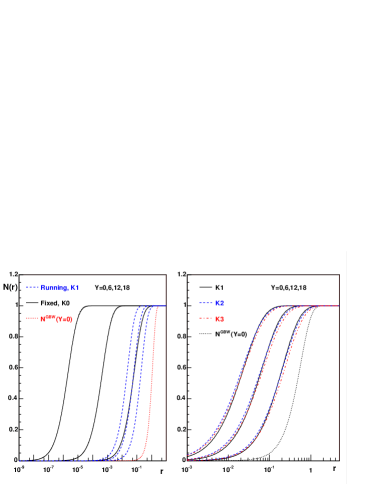
Figure 1: Solutions of the BK equation for GBW initial condition (dotted line) for rapidities $Y=6$, 12 and 18 with $\bar{\alpha}_{0}=0.4$. Left plot: Evolution with fixed ($K0$, solid lines) and running coupling ($K1$, dashed lines). Right plot: evolution with running coupling for kernel modifications $K1$ (solid lines), $K2$ (dashed lines) and $K3$ (dashed-dotted lines).

3.2 Geometrical scaling

In the limit $Y\to\infty$, the solutions of the BK evolution are no longer functions of the variables $r$ and $Y$ separately, but instead depend on a single scaling variable

$$\tau\equiv r\,Q_{s}(Y)\,.$$ (8)

The saturation momentum $Q_{s}(Y)$ determines the transverse momentum below which the unintegrated gluon distribution is saturated. It can be characterized by the position of the falloff in $N(r)$, e.g. via the definition

$$N(r=1/Q_{s}(Y),Y)=\kappa,$$ (9)

where $\kappa$ is a constant which is smaller than, but of order, one. Different choices such as $\kappa=1/2$ (as in the results given below) and $\kappa=1/e$ lead to negligible differences in the determination of $Q_{s}(Y)$.

The accuracy of scaling at small $r$ can be checked by comparison with the analytical scaling forms, for fixed and running coupling respectively, proposed in Mueller:2002zm :

$$f^{1)}(\tau)=a\tau^{2\gamma}\left(\ln{\tau^{2}}+\delta\right)\,,$$ (10)

$$f^{2)}(\tau)=a\tau^{2\gamma}\left(\ln{\tau^{2}}+{1\over\gamma}\right)\,.$$ (11)

Here, $1-\gamma$ is usually called the anomalous dimension which governs the leading large-$k$ behaviour of the unintegrated gluon distribution.

We determine $\gamma$ from a fit of our numerical results to the functions (10) and (11) in the $Y$-independent region $10^{-5}<\tau<10^{-1}$, i.e. for $10^{5}\,Q_{s}>1/r>10\,Q_{s}$, with $a$, $\gamma$ and $\delta$ as free parameters. The results given below were found to be insensitive to a variation of the lower limit of this fitting range.

For the case of fixed coupling constant, we find that the function $f^{1)}$ provides a very good fit to the evolved solutions. In Figure 2, we show the fit values of the parameter $\gamma$, obtained for fixed coupling constant from the evolution of different initial conditions $N^{GBW}$, $N^{MV}$, and $N^{AS}$ for different values of $c$. At initial rapidity, these distributions have widely different anomalous dimensions but evolution drives them to a common value, $\gamma\simeq 0.65$, which lies close to the theoretically conjectured one Iancu:2002tr ; Mueller:2002zm of $0.628$. For a small fixed coupling constant $\bar{\alpha}_{0}=0.2$, this asymptotic behaviour is reached at $Y\sim 70$, while for a larger coupling constant $\bar{\alpha}_{0}=0.4$ the approach to this asymptotic value takes half the length of evolution (results not shown). For fixed coupling solutions, $f^{2)}$ does not provide a good fit to our numerical results.

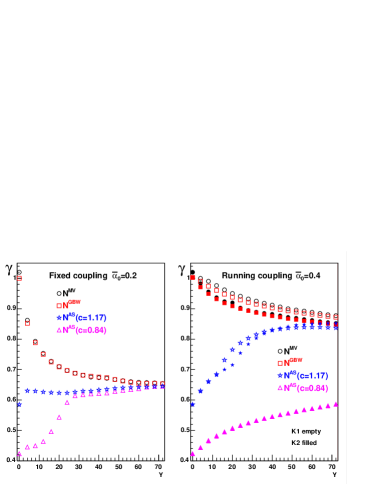
Figure 2: The rapidity dependence of the parameter $\gamma$, characterizing the anomalous dimension $1-\gamma$, as determined by a fit of (10) to the BK solutions for different initial conditions: GBW (squares), MV (circles), and AS with $c=1.17$ (stars) and $c=0.84$ (triangles). Left plot: results for fixed coupling with $\bar{\alpha}_{0}=0.2$. Right plot: results for running coupling with $\bar{\alpha}_{0}=0.4$ and two versions of the kernel $K1$ (empty symbols) and $K2$ (filled symbols).

We have repeated this comparison for all running coupling prescriptions. We found that both $f^{1)}$ and $f^{2)}$ provide good fits and yield very similar values of $\gamma$. The results for $K3$ are numerically indistinguishable from those for $K2$ and will not be shown in what follows. Also, the value of $\gamma$ was found to be independent of the coupling constant $\bar{\alpha}_{0}$ at $r\to\infty$. In Figure 2, we show the values of $\gamma$ extracted from a fit to $f^{1)}$. Irrespective of the initial condition, they approach a common asymptotic value $\gamma\sim 0.85$. While our numerical findings for $N^{AS}$ with $c=0.84$ are not inconsistent with the approach to this asymptotic value, no firm conclusions can be drawn. This initial condition just starts too far away from the asymptotic scaling solution to reach it within the numerically accessible rapidity range. In this case, the monotonic increase of $\gamma$ with rapidity at large $Y$ is smaller than the increase for $N^{AS}$ with $c=1.17$ at comparable values of $\gamma$, indicating that the rapidity evolution of the anomalous dimension depends in general not only on the small-$r$ behaviour, but on the full shape of the scattering probability.

The value $\gamma\sim 0.85$ is considerably larger than the one found in fixed coupling evolution. This is in agreement with previous numerical results Braun:2003un but in contrast to theoretical expectations Iancu:2002tr ; Mueller:2002zm ; Triantafyllopoulos:2002nz which predict the same value of $\gamma$ for the fixed and running coupling cases. As an additional check, we have performed running coupling evolution from an initial condition given by the solution at large rapidity of fixed coupling evolution (for which $\gamma\simeq 0.65$). We find that even with this initial condition, running coupling evolution leads to a value of $\gamma\sim 0.85$.

It has been argued Iancu:2002tr ; Mueller:2002zm that expressions (10) and (11) are only valid for values of $\tau$ inside the scaling window, $\tau_{\rm sw}\sim\Lambda_{QCD}/Q_{s}(Y)<\tau\lesssim 1$ with $Y_{0}$ the initial rapidity, and that the dipole scattering probability returns to the double-leading-log (DLL) expression

$$N^{DLL}(r)=a(Y)\,r^{2}\,[-\ln{(r^{2}\Lambda^{2})}]^{-3/4}\times\\ \times\exp{\left[b(Y)\sqrt{-\ln{(r^{2}\Lambda^{2})}}\,\right]}\,,$$ (12)

with $a(Y)\propto Y^{1/4}$ and $b(Y)\propto\sqrt{Y}$, for values $\tau<\tau_{\rm sw}$. We have checked that this form provides a good fit (fit and numerical solution differ by less than $\pm 10$%) to the fixed coupling solution of BK for $\tau<\tau_{\rm sw}=\Lambda/Q_{s}(Y)$, $\Lambda\sim 0.2$ GeV, see Figure 3. Our comparison is limited to rapidities $Y\leq 20$, since the scaling window starts to extend over the entire numerically accessible $r$-space for $Y>20$. Up to $Y=20$, the coefficients $a(Y)$ and $b(Y)$ follow the expected DLL $Y$-behaviour, see Figure 3. However, the scaling ansatz $f^{1)}$ provides an equally good fit to the BK solutions for $\tau<\tau_{\rm sw}$. This is the reason why in previous numerical studies Albacete:2003iq no upper bound for a scaling window was found. When the solutions of BK are fitted to $f^{1)}$ within the scaling window, the values of $\gamma$ at $Y=0$ for both initial conditions are $\lesssim 20$% smaller than those found when the fit is done within a fixed $\tau$-window. But for larger $Y$ the values of $\gamma$ extracted from fits within either the scaling window or some fixed $\tau$-window approach each other and quickly coincide.

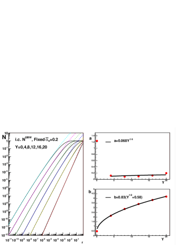
Figure 3: Plot on the left: solutions of the BK equation (solid lines) with GBW initial condition and fixed coupling $\bar{\alpha}_{s}=0.2$ compared to fits (dashed lines) to the DLL expression (12), for rapidities $Y=0$, 4, 8, 12, 16 and 20 (curves from right to left). Plots on the right: values of the coefficients $a(Y)$ and $b(Y)$ (circles) in the DLL expression versus $Y$, compared to fits (curves) to the functional form suggested by DLL.

3.3 Rapidity dependence of the saturation scale

In the scaling region and for large rapidity (where $Q_{s}(Y)\gg\Lambda_{QCD}$), the rapidity dependence of the saturation scale is determined Iancu:2002tr by

$$\frac{\partial\ln{\left[Q^{2}_{s}(Y)/\Lambda^{2}\right]}}{\partial Y}=d\,\bar{\alpha}_{s}\,,$$ (13)

where the numerical value of

$$d=\int{d^{2}\tau d^{2}\tau_{1}\over 2\pi^{2}}\,{1\over\tau_{1}^{2}\tau_{2}^{2}}\,[N(\tau_{1})+N(\tau_{2})-N(\tau)-N(\tau_{1})N(\tau_{2})]$$ (14)

can only be found once the scaling solution $N(\tau)$ is known.

For a fixed coupling constant, the saturation scale grows exponentially with rapidity

$$Q_{s}^{2}(Y)=Q_{0}^{2}\,\exp{\left[\Delta Y\right]},$$ (15)

where $\bar{\alpha}_{s}=\bar{\alpha}_{0}=$ constant, $\Delta=d\bar{\alpha}_{0}$ and $Q^{2}_{0}=Q^{2}_{s}(Y=0)$ (i.e., the evolution starts at $Y=0$).

For running coupling, the momentum scale is expected to be $\sim Q_{s}(Y)$, suggesting the substitution $\bar{\alpha}_{s}\to\bar{\alpha}_{s}(Q_{s}(Y))$ in Equation (13). This leads to Iancu:2002tr

$$Q_{s}^{2}(Y)=\Lambda^{2}\,\exp{\left[\Delta^{\prime}\sqrt{Y+X}\right]},$$ (16)

where $(\Delta^{\prime})^{2}=24N_{c}d/\beta_{0}$ and $X=(\Delta^{\prime})^{-2}\ln{(Q_{0}^{2}/\Lambda^{2})}$.

The $Y$-dependence of $Q_{s}^{2}$ for several initial conditions and for different choices of $\bar{\alpha}_{0}$, calculated for all the kernels considered in this work, is shown in Figure 4.

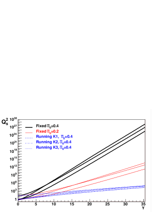
Figure 4: The rapidity dependence of the saturation momentum $Q_{s}^{2}$ for fixed $\bar{\alpha}_{s}=0.4$ (thick solid), fixed $\bar{\alpha}_{s}=0.2$ (thin solid), and running coupling with $\bar{\alpha}_{0}=0.4$ for kernels $K1$ (dashed), $K2$ (dashed-dotted) and $K3$ (dotted lines). For each group, lines from top to bottom in the rightmost side correspond to initial conditions AS with $c=1.17$, MV and GBW.

The rise of $Q_{s}^{2}$ is much faster for fixed than running coupling, in accordance with (15) and (16) and as already observed in Lublinsky:2001yi ; Golec-Biernat:2001if ; Triantafyllopoulos:2002nz ; Braun:2003un ; Rummukainen:2003ns ; Kutak:2004ym ; Khoze:2004hx ; Chachamis:2004ab

For fixed coupling constant, $Q_{s}^{2}$ exhibits with good accuracy an exponential behaviour for high-enough values of $Y$. The value of the slope extracted from a fit to the function (15) is $\Delta\simeq 1.83$ for $\bar{\alpha}_{0}=0.4$. As expected, for $\bar{\alpha}_{0}=0.2$ this value is reduced by a factor two, $\Delta\simeq 0.91$. For the constant (14), we find $d\simeq 4.57$, in agreement with previous numerical studies at very high rapidities Albacete:2003iq but slightly smaller than the theoretical expectation $d=4.88$ Iancu:2002tr ; Mueller:2002zm .

For the case of a running coupling constant, an exponential fit can be done only for a very limited $Y$-region. For example, for $Y\sim 10$ we find a logarithmic slope $\sim 0.28$ for GBW or MV initial conditions with $Q_{0}\sim 1$ GeV, in agreement with the results of Triantafyllopoulos:2002nz but smaller than the values found in Khoze:2004hx (see also Kutak:2004ym ; Chachamis:2004ab ). The exponential function (15) is unable to fit the full $Y$-range. In contrast, the weaker rapidity dependence of (16) does provide a good fit in the full $Y$-range. The fit to (16) yields $\Delta^{\prime}\simeq 3.2$, while the theoretical expectation Iancu:2002tr ; Mueller:2002zm is slightly larger, $\Delta^{\prime}=3.6$.

3.4 Nuclear size dependence of the saturation scale

The nuclear size enters the initial condition. Here, we examine the effect of BK evolution on the initial nuclear size dependence of the saturation scale. Figure 5 summarises our results.

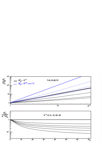
Figure 5: Upper plot: $Q_{sA}^{2}/Q_{sp}^{2}$ versus $A^{1/3}$ for initial conditions GBW ($Q_{sA}^{2}(Y=0)\propto A^{1/3}$, solid) and AS with $c=1.17$ ($Q_{sA}^{2}(Y=0)\propto A^{2/3c}$, dashed lines); thick lines are the results for $Y=0$ in the running coupling case and for all rapidities in fixed coupling; for running coupling, different rapidities $Y=10$, 40 and 72 (thin lines) are shown from top to bottom for each initial condition. Lower plot: $Q_{sA}^{2}/(A^{1/3}Q_{sp}^{2})$ versus $Y$ for GBW with $A^{1/3}=3$, 6, 10, 20 and 50 with the same line convention as the upper plot (the results for fixed coupling have been obtained for $Y<36$ and extrapolated as a constant equal to 1). In all plots $\bar{\alpha}_{0}=0.4$ and in the running coupling case the kernel $K1$ has been used.

In the fixed coupling case, the initial $A$-dependence of the saturation scale is preserved, irrespectively of whether this dependence is $\propto A^{1/3}$ as for the GBW or MV initial conditions (which produces numerical results for the $A$-dependence which are very close to those obtained for GBW), or whether it differs from $\propto A^{1/3}$ due to an anomalous dimension as the one included in the AS initial condition. This is in agreement with the theoretical expectation that, given the dilatation invariance of the BK equation (3), any nuclear dependence present in the initial condition can be scaled out.

The evolution with running coupling is seen to reduce the $A$-dependence with increasing rapidity. If fitted in a wide rapidity range, the dependence of $\ln{[Q_{sA}^{2}(Y)/Q_{sp}^{2}(Y)]}$ on $Y$ is $\sim Y^{-0.4}$. However, for large values of $A$ and $Y$, the decrease with increasing $Y$ is $\propto 1/\sqrt{Y}$ and thus well described by Mueller:2003bz

$$\ln{{Q_{sA}^{2}(Y)\over Q_{sp}^{2}(Y)}}\simeq{\ln^{2}{\left[{h\,Q_{s}^{2}(Y=0)\over\Lambda^{2}}\right]}\over 2\sqrt{(\Delta^{\prime})^{2}Y}}\,,$$ (17)

where $h\,Q_{s}^{2}(Y=0)$ is the initial saturation momentum for the nucleus, and $(\Delta^{\prime})^{2}$ is defined below Equation (16).

4 Geometric scaling and experimental data

4.1 Geometric scaling in lepton-hadron collisions

Following Armesto:2004ud and motivated by the previous sections, let us assume that both the energy and the nuclear size (or centrality) dependence of the scattering amplitude $N({\bf r},x;{\bf b})$ can be encoded in the saturation scale $Q_{s,h}(x,{\bf b})$ for any $h$ (proton or nucleus). Then, the cross section (1) can be written as

$$\sigma_{T,L}^{\gamma^{*}h}(x,Q^{2}) = \pi R_{h}^{2}\int d{\bf r}\int_{0}^{1}dz|\Psi_{T,L}^{\gamma^{*}}(Q^{2},{\bf r},z)|^{2}$$ (18)

$$\times 2\int d{\bf\bar{b}}\,N_{h}(rQ_{\rm s,h}(x,{\bf\bar{b}}))\,.$$

In this case, since $|\Psi_{T,L}^{\gamma^{*}}(Q^{2},{\bf r},z)|^{2}$ is proportional to $Q^{2}$ times a function of ${\bf r}^{2}Q^{2}$, the cross section is only a function of $\tau_{h}^{2}=Q^{2}/Q_{\rm s,h}^{2}(x)$. This geometric scaling was found to describe all lepton-proton data with $x<0.01$ Stasto:2000er . In order to compare protons and different nuclei Armesto:2004ud one needs to make some assumptions about the impact parameter dependence. Here, we have assumed that all the $b$ dependence can be scaled by the nuclear radius of the hadronic target $h$, ${\bf\bar{b}}={\bf b}/\sqrt{\pi R_{h}^{2}}$, with $R_{A}=(1.12A^{1/3}-0.86A^{-1/3})$ fm. Then, the condition for geometric scaling in lepton-nucleus data is

$$\frac{\sigma^{\gamma^{*}A}(\tau_{A})}{\pi R_{A}^{2}}=\frac{\sigma^{\gamma^{*}p}(\tau_{A})}{\pi R_{p}^{2}}\,.$$ (19)

For the $A$-dependence, we make the ansatz that the saturation scale in the nucleus grows with the ratio of the transverse parton densities to some power $1/\delta$, which we take as a free parameter

$$Q_{\rm s,A}^{2}=Q_{\rm s,p}^{2}\left(\frac{A\pi R_{p}^{2}}{\pi R_{A}^{2}}\right)^{\frac{1}{\delta}}\Rightarrow\tau_{A}^{2}=\tau_{p}^{2}\left(\frac{\pi R_{A}^{2}}{A\pi R_{p}^{2}}\right)^{\frac{1}{\delta}}.$$ (20)

Here, $\pi R_{p}^{2}$ is the second free parameter to be fixed by the data.

For the proton case we take the Golec-Biernat and Wüsthoff (GBW) parametrization Golec-Biernat:1998js , $Q_{\rm s,p}^{2}=(\bar{x}/x_{0})^{-\lambda}$ in GeV², $x_{0}=3.04\cdot 10^{-4}$ and $\lambda=0.288$. This parametrization shows geometric scaling as can be seen in Fig. 6. In order to proceed to the nuclear case, we need a functional form of the scaling curve. The data proton are seen to be well parametrized by Armesto:2004ud

$$\sigma^{\gamma^{*}p}(x,Q^{2})\equiv\Phi(\tau_{p}^{2})=\bar{\sigma}_{0}\left[\gamma_{E}+\Gamma\left(0,\xi\right)+\ln\xi\right]\,,$$ (21)

where $\gamma_{E}$ is the Euler constant, $\Gamma\left(0,\xi\right)$ the incomplete $\Gamma$ function and $\xi=a/\tau_{p}^{2b}$, with $a=1.868$ and $b=0.746$. The normalization is fixed by $\bar{\sigma}_{0}=40.56$ mb.

To determine $Q_{\rm s,A}^{2}$, we use Eqs. (19) and (20) and compare the functional shape (21) to the available experimental data for $\gamma^{*}A$ collisions with $x\leq 0.0175$ Adams:1995is ; Arneodo:1995cs ; Arneodo:1996rv , using $\xi=a/\tau_{A}^{2b}$. We obtain $\delta=0.79\pm 0.02$ and $\pi R_{p}^{2}=1.55\pm 0.02$ fm² for a $\chi^{2}/{\rm dof}=0.95$ (see Fig. 6 for the comparison). Notice that these parameters translate into a growth of the saturation scale faster than $A^{1/3}$ for large nuclei. If we impose $Q_{\rm s,A}^{2}\sim A^{1/3}$ in the fit, a much worse value of $\chi^{2}/{\rm dof}=2.35$ is obtained. We conclude that the small-$x$ experimental data on $\gamma^{*}A$ collisions favours an increase of $Q_{\rm s,A}^{2}$ faster than $A^{1/3}$. The numerical coincidence $b\simeq\delta$ is consistent with the absence of shadowing in nuclear parton distributions at $Q^{2}\gg Q_{\rm s,A}^{2}$.

Figure 6: Geometric scaling for $\gamma^{*}p$ (upper panel, data from proton ), $\gamma^{*}A$ (middle panel, data from Adams:1995is ; Arneodo:1995cs ) and the ratio of data for $\gamma^{*}A$ over the prediction from (21) (lower panel). As an additional check, the lower plot also shows data for $\gamma^{*}A$ normalized with respect to $\gamma^{*}C$ Arneodo:1996rv , and divided by the corresponding prediction from Eq. (21).

4.2 Geometric scaling and multiplicities in AA collisions

In Armesto:2004ud a simple formula for multiplicities in symmetric colliding systems at central rapidities has been proposed:

$$\frac{1}{N_{\rm part}}\frac{dN^{AA}}{d\eta}\Bigg{|}_{\eta\sim 0}=N_{0}\sqrt{s}^{\lambda}N_{\rm part}^{\frac{1-\delta}{3\delta}}\,.$$ (22)

An easy way to derive this formula is to take, as the starting point, the factorized expression Gribov:tu for gluon production

$$\frac{dN^{AB}_{g}}{dyd{\bf p}_{t}d{\bf b}}\propto\frac{\alpha_{S}}{{\bf p}_{t}^{2}}\int d{\bf k}\ \phi_{A}(y,{\bf k}^{2},{\bf b})\,\phi_{B}\left(y,({\bf k}-{\bf p}_{t})^{2},{\bf b}\right)\,,$$ (23)

where $\phi_{h}(y,{\bf k},{\bf b})=\int d{\bf r}\,\exp\{i{\bf r\cdot k}\}\,N_{h}({\bf r},x;{\bf b})/(2\pi r^{2})$ facto .

If one assumes geometric scaling for the parton distributions, $\phi_{A}(y,{\bf k}^{2},{\bf b})$$\equiv$ $\phi({\bf k}^{2}/Q_{\rm s,A}^{2}(y,{\bf b}))$, we obtain

$$\frac{dN^{AA}_{g}}{dy}\Bigg{|}_{y\sim 0}\propto\int\frac{d{\bf p}_{t}}{{\bf p}_{t}^{2}}d{\bf k}d{\bf b}\ \phi\left(\frac{{\bf k}^{2}}{Q_{\rm s,A}^{2}}\right)\,\phi\left(\frac{({\bf k}-{\bf p}_{t})^{2}}{Q_{\rm s,A}^{2}}\right)$$

$$=Q_{\rm s,A}^{2}\pi R_{A}^{2}\int\frac{d{\bf s}}{{\bf s}^{2}}d{\bf\tau}d{\bar{\bf b}}\ \phi({\bf\tau}^{2})\,\phi\left(({\bf\tau}-{\bf s})^{2}\right),$$ (24)

where the integrand is a constant. This proportionality between the total multiplicities and the saturation scale is shared by other models of hadroproduction Gribov:tu ; facto ; Eskola:1999fc ; Kovchegov:2000hz . It is important to notice, however, that for the case of geometric scaling, Eq. (22) is more general than the factorized form (23). Indeed, any functional shape of the integrand will lead to the same result providing geometric scaling holds. In order to recover Eq. (22), the energy dependence of the saturation scale in (24) is given by the GBW parameter $\lambda=0.288$; for its centrality dependence we use the known proportionality in symmetric A+A collisions between the number $N_{\rm part}$ of participant nucleons and the nuclear size $A$ and $Q_{\rm s,A}^{2}\propto A^{1/3\delta}$, with $\delta=0.79\pm 0.02$. In this way, the energy and centrality dependences are determined by parameters fitted to $\gamma^{*}-p$ and $\gamma^{*}-A$ respectively. In all these models, the hadron yield is assumed to be proportional to the yield of produced partons. The remaining normalization constant is fixed to $N_{0}=0.47$ in order to reproduce PHOBOS data, see Fig. 7. It is interesting that even the ${\bar{p}}$+$p$ data (protmult , as quoted in Back:2002uc ) at $\sqrt{s}=$ 19.6 and 200 GeV are accounted for. Eq. (22) implies that the energy and the centrality dependence of the multiplicity factorize, in agreement with the results by PHOBOS Back:2002uc .

Figure 7: Energy and centrality dependence of the multiplicity of charged particles in Au+Au collisions (22) compared to PHOBOS data Back:2002uc . Also shown in the lower panel are the ${\bar{p}}$+$p$ data protmult and results for $\sqrt{s}=$ 62.5 and 5500 GeV/A.

A formula similar to Eq. (22) has been extensively employed to study multiplicities in Au+Au collisions in kln . These authors assume $Q_{\rm s,A}^{2}\propto A^{1/3}$ and an additional enhancement factor $\ln(\sqrt{s}^{\lambda}N_{\rm part}^{1/3})$ argued to come from scaling violations of the coupling constant in (23). Notice that for the accessible range of $A$, $A^{4/9}\sim A^{1/3}\,\ln(A^{1/3})$ – this being the reason why both approaches provide a fair description of the data at RHIC.

4.3 Geometric scaling and dAu data

The forward rapidity region of the RHIC experiments has become the main testing ground for saturation ideas. In this section, we check to which extent geometric scaling can account for the observed suppression on particle yields. The situation in this case is, however, more model-dependent than in the previous two cases. The reason is the existence of two different saturation scales (one for the deuteron and another one for the gold nucleus) which precludes the trivial changes of variables done before. In order to proceed, we observe that if one writes Eq. (1) in momentum space $k$, the main contribution to the cross section comes from $k\sim Q/2$. Approximating the dipole wave function (in momentum space) by $\delta(k-Q/2)$, the scaling curve (21) is (except for a normalization constant) the unintegrated gluon distribution, $\phi_{A}(k=Q/2)\simeq\Phi(\tau_{A})$, with $\tau_{A}=k^{2}/4\bar{Q}_{\rm s,A}^{2}$. For the case of particle production in dAu collisions, the gluon saturation scale $\bar{Q}_{\rm s,A}^{2}=N_{c}Q_{\rm s,A}^{2}/C_{F}$ needs to be used. Now, if the parton distribution in the deuteron falls off sufficiently quickly, $\phi_{d}\sim 1/k_{t}^{n}$, $n\gg 1$, we obtain from Eq. (23)

$$\frac{\frac{dN^{\rm dAu}_{c_{1}}}{N_{\rm coll_{1}}d\eta d^{2}p_{t}}}{\frac{dN^{\rm dAu}_{c_{2}}}{N_{\rm coll_{2}}d\eta d^{2}p_{t}}}\approx\frac{N_{\rm coll_{2}}\phi_{A}(p_{t}/Q_{\rm s,c_{1}})}{N_{\rm coll_{1}}\phi_{A}(p_{t}/Q_{\rm s,c_{2}})}\approx\frac{N_{\rm coll_{2}}\Phi(\tau_{c_{1}})}{N_{\rm coll_{1}}\Phi(\tau_{c_{2}})}\,$$ (25)

for the centrality classes $c_{1}$, $c_{2}$. This simple formula relates the suppression measured in lepton-nucleus collisions to that in d+Au. For the comparison in Fig. 8 to data Arsene:2004ux on the normalized yields of central and semi-central over peripheral d+Au collisions, we use the number of nucleon-nucleon collisions $N_{\rm coll}$ in different centrality bins Arsene:2004ux with $N_{\rm coll_{1}}=13.6\pm 0.3$, $7.9\pm 0.4$ and $N_{\rm coll_{2}}=3.3\pm 0.4$. Only the two most forward rapidities $\eta=2.2$ and 3.2 are compared. This simplistic analysis indicates that the suppression of particle yields in forward rapidity measured in d+Au collisions is in agreement, through geometric scaling, with the nuclear shadowing measured in lepton-nucleus collisions. The connection between the small $x$- and $A$-dependence of parton distribution functions, and the suppression of normalized yields in d+Au collisions Arsene:2004ux at forward rapidity has been discussed in several recent works Albacete:2003iq ; others . Eq. (25) contributes to this discussion by illustrating to what extent the suppression of high-$p_{t}$ particles in d+Au at RHIC can be accounted for by the shadowing in $\gamma^{*}A$ collisions, see Eq. (21).

Figure 8: Normalized ratios of central and semi-central to peripheral d+Au collisions measured by BRAHMS Arsene:2004ux compared to results from Eq. (25). The bands represent the uncertainty in the determination of $N_{\rm coll}$ Arsene:2004ux .

5 Comparison of data and theory and conclusions

The two main properties of the BK evolution are the existence of a scale which indicates the presence of a saturated region and the existence of a scaling solution at asymptotic energies. The analytic form of the asymptotic solution is only known for some ranges of the dipole size. Here we have presented a numerical analysis of the BK equations without impact parameter dependence. In order to study the possible effects of next-to-leading-log corrections to the BK equation we have included the running of the coupling constant, using several prescriptions. Our results confirm the existence of a scaling solution also for the running coupling case. Most of our numerical results agree with the analytical estimations. Namely, the evolution in rapidity of the saturation scale has been found to be exponential for the case of fixed coupling and slower (the exponential of a square root) for the running coupling case and with parameters in agreement with analytical estimates; the nuclear size dependence of the saturation scale has been found to be preserved in the fixed coupling case and to disappear asymptotically in the running coupling case; the small-$r$ behaviour of the scaling solutions reproduces the anomalous dimension found analytically for the case of a fixed coupling, but it is found to be different (in disagreement with analytical estimations) in the running coupling case.

If the dynamics of the BK equations is relevant for the present experimentally accessible regimes, the above properties should be realized in the data. The observation Stasto:2000er that all the available data on lepton-proton scattering with $x<0.01$ can be described by a single variable $\tau^{2}=Q^{2}/Q_{\rm s,p}^{2}$ is reminiscent of the existence of a scaling solution. The energy dependence of the saturation scale extracted from a fit to experimental data Golec-Biernat:1998js is too small compared with the results of BK with fixed coupling. It is, however, in approximate agreement with the running coupling case if one is restricted to a small range of energies. In the nuclear case, we have found Armesto:2004ud that a similar geometric scaling of the nuclear data is possible by encoding the nuclear size in the saturation scale. The $A$-dependence is, however, different from the usually assumed $A^{1/3}$ and turns out to be stronger, $\sim A^{4/9}$. If this result is not a numerical accident, this behaviour could only have a dynamical origin (the geometrical behaviour of $Q_{\rm s,A}^{2}$ is $A^{1/3}$). This is not in disagreement with the solutions we have obtained from the BK equations, but the relation is obscure: the $A$-dependence of the saturation scale is preserved (i.e. it is the same as in the initial conditions) for the fixed coupling case, but disappears for the running coupling case. The nuclear size dependence is, however, expected to be modified when an appropriate treatment of the impact parameter is taken into account in the BK equation bdeprc .

We have also found that a simple explanation for the centrality dependence of the multiplicities measured in symmetric systems at central rapidities is possible with the nuclear size dependence of the saturation scale obtained from lepton-nucleus data. In the presence of a geometric scaling, these multiplicities are proportional to $Q_{\rm s,A}^{2}$. This translates into a proportionality of the multiplicities with the number of participants for the geometrical estimation $Q_{\rm s,A}^{2}\sim A^{1/3}$. The $A$-dependence $Q_{\rm s,A}^{2}\sim A^{4/9}$ gives, however, a nice description of the experimental data. As a final check, we have found a striking similarity of the suppression of nuclear yields in forward d+Au collisions measured by the BRAHMS collaboration at RHIC and the nuclear shadowing measured in lepton-nucleus experiments. All these observations are in agreement with the interpretation of the data in terms of saturation physics, but the existence of a numerical accident cannot be excluded. A quantitative description of the experimental data with explicit use of QCD evolution equations will be needed in order to establish the relevance of the saturation effects.

- (1) N. N. Nikolaev and B. G. Zakharov, Z. Phys. C 49, 607 (1991); A. H. Mueller, Nucl. Phys. B 415, 373 (1994).
- (2) I. Balitsky, Nucl. Phys. B 463, 99 (1996); Y. V. Kovchegov, Phys. Rev. D 60, 034008 (1999).
- (3) A. Kovner, J. G. Milhano and H. Weigert, Phys. Rev. D 62, 114005 (2000).
- (4) J. L. Albacete, N. Armesto, J. G. Milhano, C. A. Salgado and U. A. Wiedemann, Phys. Rev. D 71 (2005) 014003.
- (5) K. Golec-Biernat and M. Wusthoff, Phys. Rev. D 59, 014017 (1999).
- (6) L. D. McLerran and R. Venugopalan, Phys. Rev. D 49, 2233 (1994); L. D. McLerran and R. Venugopalan, Phys. Rev. D 49, 3352 (1994); L. D. McLerran and R. Venugopalan, Phys. Rev. D 50 (1994) 2225.
- (7) A. H. Mueller and D. N. Triantafyllopoulos, Nucl. Phys. B 640, 331 (2002).
- (8) E. Iancu, K. Itakura and L. McLerran, Nucl. Phys. A 708, 327 (2002).
- (9) M. A. Braun, Phys. Lett. B 576, 115 (2003).
- (10) D. N. Triantafyllopoulos, Nucl. Phys. B 648, 293 (2003).
- (11) J. L. Albacete, N. Armesto, A. Kovner, C. A. Salgado and U. A. Wiedemann, Phys. Rev. Lett. 92, 082001 (2004).
- (12) M. Braun, Eur. Phys. J. C 16, 337 (2000).
- (13) N. Armesto and M. A. Braun, Eur. Phys. J. C 20, 517 (2001).
- (14) K. Golec-Biernat, L. Motyka and A. M. Stasto, Phys. Rev. D 65, 074037 (2002).
- (15) M. Lublinsky, E. Gotsman, E. Levin and U. Maor, Nucl. Phys. A 696 (2001) 85.
- (16) K. Rummukainen and H. Weigert, Nucl. Phys. A 739, 183 (2004).
- (17) K. Kutak and A. M. Stasto, arXiv:hep-ph/0408117.
- (18) V. A. Khoze, A. D. Martin, M. G. Ryskin and W. J. Stirling, Phys. Rev. D 70 (2004) 074013.
- (19) G. Chachamis, M. Lublinsky and A. Sabio Vera, Nucl. Phys. A 748 (2005) 649.
- (20) A. H. Mueller, Nucl. Phys. A 724 (2003) 223.
- (21) N. Armesto, C. A. Salgado and U. A. Wiedemann, Phys. Rev. Lett. 94 (2005) 022002.
- (22) A. M. Stasto, K. Golec-Biernat and J. Kwiecinski, Phys. Rev. Lett. 86, 596 (2001).
- (23) J. Breitweg et al., Phys. Lett. B 487, 53 (2000); C. Adloff et al., Eur. Phys. J. C 21, 33 (2001); C. Adloff et al., Nucl. Phys. B 497, 3 (1997); M. R. Adams et al., Phys. Rev. D 54, 3006 (1996).
- (24) M. R. Adams et al., Z. Phys. C 67, 403 (1995).
- (25) M. Arneodo et al., Nucl. Phys. B 441, 12 (1995).
- (26) M. Arneodo et al., Nucl. Phys. B 481, 3 (1996); ibid. B 481, 23 (1996).
- (27) L. V. Gribov, E. M. Levin and M. G. Ryskin, Phys. Rept. 100, 1 (1983).
- (28) M. A. Braun, Phys. Lett. B 483, 105 (2000); Y. V. Kovchegov and K. Tuchin, Phys. Rev. D 65, 074026 (2002); R. Baier, A. H. Mueller and D. Schiff, Nucl. Phys. A 741, 358 (2004).
- (29) K. J. Eskola, K. Kajantie, P. V. Ruuskanen and K. Tuominen, Nucl. Phys. B 570, 379 (2000).
- (30) Y. V. Kovchegov, Nucl. Phys. A 692, 557 (2001).
- (31) W. Thome et al., Nucl. Phys. B 129, 365 (1977); G. J. Alner et al., Z. Phys. C 33, 1 (1986).
- (32) B. B. Back et al., Phys. Rev. C 65, 061901 (2002); B. B. Back et al. [PHOBOS Collaboration], Phys. Rev. C 70 (2004) 021902.
- (33) D. Kharzeev and M. Nardi, Phys. Lett. B507, 121 (2001); D. Kharzeev and E. Levin, Phys. Lett. B523, 79 (2001).
- (34) I. Arsene et al. [BRAHMS Collaboration], Phys. Rev. Lett. 93 (2004) 242303.
- (35) D. Kharzeev, E. Levin and L. McLerran, Phys. Lett. B 561, 93 (2003); R. Baier, A. Kovner and U. A. Wiedemann, Phys. Rev. D 68, 054009 (2003); D. Kharzeev, Y. V. Kovchegov and K. Tuchin, Phys. Rev. D 68, 094013 (2003);
- (36) K. Golec-Biernat and A. M. Stasto, Nucl. Phys. B 668, 345 (2003); E. Gotsman et al., hep-ph/0401021.