QCD at Low Energies.

Abstract

The modern status of basic low energy QCD parameters is reviewed. It is demonstrated, that the recent data allows one to determine the light quark mass ratios with an accuracy 10-15%. The general analysis of vacuum condensates in QCD is presented, including those induced by external fields. The QCD coupling constant $\alpha_{s}(m^{2}_{\tau})$ is found from the $\tau$-lepton hadronic decay rate. The contour improved perturbation theory includes the terms up to $\alpha^{4}_{s}$. The influence of instantons on $\alpha_{s}(m^{2}_{\tau})$ determination is estimated. V-A spectral functions of $\tau$-decay are used for construction of the V-A polarization operator $\Pi_{V-A}(s)$ in the complex $s$-plane. The operator product expansion (OPE) is used up to dimension D=10 and the sum rules along the rays in the complex $s$-plane are constructed. This makes it possible to separate the contributions of operators of different dimensions. The best values of quark condensate and $\alpha_{s}\langle 0|\bar{q}q|0\rangle^{2}$ are found. The value of quark condensate is confirmed by considering the sum rules for baryon masses. Gluon condensate is found in four ways: by considering of V+A polarization operator based on the $\tau$-decay data, by studying the sum rules for polarization operators momenta in charmonia in the vector, pseudoscalar and axial channels. All of these determinations are in agreement and result in $\langle(\alpha_{s}/\pi)G^{2}\rangle=0.005\pm 0.004~{}GeV^{4}$. Valence quark distributions in proton are calculated in QCD using the OPE in proton current virtuality. The quark distributions agree with those found from the deep inelastic scattering data. The same value of gluon condensate is favoured.

Content

1   Introduction
2   The Masses of Light Quarks
3   Condensates
3.1 General Properties
3.2 Condensates, Induced by External Fields
4   Test of QCD at Low Energies on the Basis of $\tau$-decay Data
4.1 Determination of $\alpha_{s}(m^{2}_{\tau})$
4.2 Instanton Corrections
4.3 Comparison with Other Approaches
5   Determination of Condensates from Spectral Functions of $\tau$-decay
5.1 Determination of Quark Condensate from V-A Spectral Function.
5.2 Determination of Condensate from V+A and V Structure Functions.
6   Determination of Quark Condensate from QCD Sum Rules

for Nucleon Mass
7   Gluon Condensate and Determination of Charmed Quark Mass

from Charmonium Spectrum
7.1 The Method of Moments. The Results
7.2 The Attempts to Sum Up the Coulomb-like Corrections
8   Valence Quark Distributions in Nucleon at Low $Q^{2}$ and the Condensates.
9   Conclusion
10  Acknowledgements

PACS: 11.55 Hx; 12.38 Lg; 133.35 Dx

Keywords: Quantum chromodynamics; Condensates, Operator Product Expansion.

1 Introduction

Nowadays, it is reliably established that the true (microscopic) theory of strong interaction is quantum chromodynamics (QCD), the nonabelian gauge theory of interacting quarks and gluons. The main confirmation of QCD comes from considering the processes at high energies and high momentum transfers, where, because of asymptotic freedom, the high precision of theoretical calculation is achieved and comparison with experiment confirms QCD with a very good accuracy. In the domain of low energies and momentum transfers (by such a domain in this paper I mean the domain of momentum transfers $Q^{2}\sim 1-5~{}GeV^{2}$) the situation is more complicated: the QCD coupling constant $\alpha_{s}$ is large, $\alpha_{s}\sim 0.5-0.3$ and many loops perturbative calculations are necessary. Unlike quantum electrodynamics (QED), the vacuum in QCD has a nontrivial structure: due to nonperturbative effects, non-zero fluctuations of gluonic and quark fields persist in QCD vacuum. The nontrivial vacuum structure of QCD manifests itself in the presence of vacuum condensates, analogous to those in condense matter physics (for instance, spontaneous magnetization). Therefore, $\alpha_{s}$ corrections and nonperturbative effects must be correctly accounted in QCD calculation in this domain.

At lower energies and $Q^{2}\mathrel{\mathchoice{\lower 3.6pt\vbox{\halign{$\mathsurround=0pt\displaystyle\hfil#\hfil$\cr<\crcr\sim\crcr}}}{\lower 3.6pt\vbox{\halign{$\mathsurround=0pt\textstyle\hfil#\hfil$\cr<\crcr\sim\crcr}}}{\lower 3.6pt\vbox{\halign{$\mathsurround=0pt\scriptstyle\hfil#\hfil$\cr<\crcr\sim\crcr}}}{\lower 3.6pt\vbox{\halign{$\mathsurround=0pt\scriptscriptstyle\hfil#\hfil$\cr<\crcr\sim\crcr}}}}1~{}GeV^{2}$ analytical QCD calculations are not reliable. The useful methods are: the chiral effective theory, lattice calculations and various model approaches. It is, however, very desirable to have a matching of all these approaches with QCD calculations at $Q^{2}$ about $1GeV^{2}$. To achieve this the knowledge of low energy QCD parameters is necessary.

In order to fix the notations I present here the form of QCD Lagrangian:

$$L=i~{}\sum\limits_{q}\bar{\psi}^{a}_{q}(\nabla_{\mu}\gamma_{\mu}+im_{q})\psi^{a}_{q}-\frac{1}{4}~{}G^{n}_{\mu\nu}G^{n}_{\mu\nu},$$ (1)

where

$$\nabla_{\mu} = \partial_{\mu}-ig\frac{\lambda^{n}}{2}A^{n}_{\mu}$$

$$G^{n}_{\mu\nu} = \partial_{\mu}A^{n}_{\mu}-\partial_{\nu}A^{n}_{\mu}+gf^{nml}A^{m}_{\mu}A^{l}_{\nu}$$ (2)

$\psi^{a}_{q}$ and $A^{n}_{\mu}$ are quark and gluon fields, $a=1,2,3$; $n,m,l=1,2,...8$ are colour indeces, $\lambda^{n}$ and $f^{nml}$ are Gell-Mann matrices and $f$-symbols, $m_{q}$ – are bare (current) quark masses, $q=u,d,s,c...$.

Vacuum condensates are very important in the elucidation of the QCD structure and in description of hadron properties at low energies. Condensates, particularly, quark and gluonic ones, were investigated starting from the 70-ties. Here, first, it should be noted the QCD sum rule method by Shifman, Vainshtein, and Zakharov [1], which was based on the idea of the leading role of condensates in the calculation of masses of the low-lying hadronic states. In the papers of the 70-80-ies it was assumed that the perturbative interaction constant is comparatively small (e.g., $\alpha_{s}(1GeV)\approx 0.3)$, so that it is enough to restrict oneself by the first-order terms in $\alpha_{s}$ and sometimes even disregard perturbative effects in the region of masses larger than 1 GeV. At present it is clear that $\alpha_{s}$ is considerably larger ($\alpha_{s}(1GeV)\sim 0.5$). In a number of cases there appeared the results of perturbative calculations in order $\alpha^{2}_{s}$ and $\alpha^{3}_{s}$. New, more precise experimental data at low energies had been obtained.

This review presents the modern status of QCD at low energies. In Chapter 2 the values of light quark masses are discussed. Chapter 3 contains the definition of condensates and the description of their general properties. In Chapter 4 the QCD coupling constant $\alpha_{s}$ is determined from the data on hadronic $\tau$-decay and its evolution with $Q^{2}$ (in 4-loops approximation) is given. In Chapter 5 quark and gluon condensates are found from the $\tau$-decay data on V-A, V+A and V correlators. The sum rules for nucleon mass with account of $\alpha_{s}$ corrections are analyzed in Chapter 6 and it is shown, that they are well satisfyed at the same value of quark condensate, which was found from the $\tau$-decay data. Various ways of gluon condensate determination: a) from $V+A$ correlators; b) from charmonium sum rules are considered in Chapter 7. The QCD sum rules for valence quark distributions in nucleon are presented in Chapter 8, valence $u$- and $d$-quark distributions at low $Q^{2}$ were found and the restriction on condensates were obtained. Finally, chapter 9 summarizes the state of the art of low energy QCD.

2 The masses of light quarks

The $u,d,s$ quark masses had been first estimated by Gasser and Leutwyler about 30 years ago: it was demonstrated that $m_{u},m_{d}\sim 5~{}MeV$ and $m_{s}\sim 100MeV$ [2, 3]. In 1977 Weinberg [4], using partial conservation of axial current and Dashen theorem [5] to account for electromagnetic selfenergies of mesons had proved, that the ratios $m_{u}/m_{d}$ and $m_{s}/m_{d}$ may be expressed through $K$ and $\pi$ masses:

$$\frac{m_{u}}{m_{d}}=\frac{m^{2}_{K^{+}}-m^{2}_{K^{0}}+2m^{2}_{\pi^{0}}-m^{2}_{\pi^{+}}}{m^{2}_{K^{0}}-m^{2}_{K^{+}}+m^{2}_{\pi^{+}}}$$ (3)

$$\frac{m_{s}}{m_{d}}=\frac{m^{2}_{K^{0}}+m^{2}_{K^{+}}+m^{2}_{\pi^{+}}}{m^{2}_{K^{0}}-m^{2}_{K^{+}}+m^{2}_{\pi^{+}}}$$ (4)

Numerically, (3) and (4) are equal

$$\frac{m_{u}}{m_{d}}=0.56~{}~{}~{}~{}~{}~{}~{}\frac{m_{s}}{m_{d}}=20.1$$ (5)

Basing on consideration of mass splitting in baryon octet Weinberg assumed, that $m_{s}=150MeV$ at the scale of about 1 GeV. Then

$$m_{u}=4.2MeV,~{}~{}~{}m_{d}=7.5MeV,~{}~{}~{}m_{s}=150MeV$$ (6)

at 1 GeV. The large $m_{s}/m_{d}$ ratio explains the large mass splitting in pseudoscalar meson octet. For $m^{2}_{K^{+}}/m^{2}_{\pi^{+}}$ we have $[\bar{m}=(m_{u}+m_{d})/2]$

$$\frac{m^{2}_{K^{+}}}{m^{2}_{\pi^{+}}}=\frac{m_{s}+\bar{m}}{2\bar{m}}=13$$ (7)

in a perfect agreement with experiment. The ratio $m^{2}_{\eta}/m^{2}_{\pi}$ expressed in terms of quark mass ratios is also in a good agreement with experiment.

The ratios (3),(4) were obtained in the first order in quark masses. Therefore, their accuracy is of order of accuracy of SU(3) symmetry, i.e. about 20%.

In [6] it was demonstrated that there is a relation valid in the second order in quark masses

$$\Biggl{(}\frac{m_{u}}{m_{d}}\Biggr{)}^{2}+\frac{1}{Q^{2}}\Biggl{(}\frac{m_{s}}{m_{d}}\Biggr{)}^{2}=1$$ (8)

Using Dashen theorem for electromagnetic selfenergies of $\pi$ and $K$-meson, one may express $Q$ as

$$Q^{2}_{D}=\frac{(m^{2}_{K^{0}}+m^{2}_{K^{+}}-m^{2}_{\pi^{+}}+m^{2}_{\pi^{0}})(m^{2}_{K^{0}}+m^{2}_{K^{+}}-m^{2}_{\pi^{+}}-m^{2}_{\pi^{0}})}{4m^{2}_{\pi^{0}}(m^{2}_{K^{0}}-m^{2}_{K^{+}}+m^{2}_{\pi^{+}}-m^{2}_{\pi^{0}})}$$ (9)

Numerically, $Q_{D}$ is equal: $Q_{D}=24.2$. However, Dashen theorem is valid in the first order in quark masses. The electromagnetic mass difference of $K$-mesons calculated in [7] by using Cottingham formula and in [8] by large $N_{c}$ approach increased $\Delta m_{k}=(M_{K^{+}}-M_{K^{0}})_{e.m.}$ from Dashen value $\Delta m_{k}=1.27$ MeV to $\Delta m_{k}=2.6$  MeV and, correspondingly, decreased $Q$ to $Q=22.0\pm 0.6$. The other way to find $Q$ is from $\eta\to\pi^{+}\pi^{-}\pi^{0}$ decay, using the chiral effective theory. Unfortunately, the next to leading corrections are large in this approach [9], what makes uncertain the accuracy of the results. It was found from the $\eta\to\pi^{+}\pi^{-}\pi^{0}$ decay data with the account of interaction in the final state: $Q=22.4\pm 0.9$ [10], $Q=22.7\pm 0.8$ [11] and $Q=22.8\pm 0.4$ [12] (the latter from the Dalitz plot). So, the final conclusion is that $Q$ is in the interval $21.5<Q<23.5$. (It must be mentioned that the experiment, where $\Gamma(\eta\to 2\gamma)$ and, consequently, $\Gamma(\eta\to\pi^{+}\pi^{-}\pi^{0})$ were measured by the Primakoff effect, is absent in the last edition of the Particle data [13], while it persisted in the previous ones. See [14] for the review.) The ratio $\gamma=m_{u}/m_{d}$ can also be found from the ratio of $\psi^{\prime}\to(J/\psi)\eta$ and $\psi^{\prime}\to(J/\psi)\pi^{0}$ decays [15, 16] . In [15] it was proved that

$$r=\frac{\Gamma(\psi^{\prime}\to J/\psi+\pi^{0})}{\Gamma(\psi^{\prime}\to J/\psi+\eta)}=3\Biggl{(}\frac{1-\gamma}{1+\gamma}\Biggr{)}^{2}\Biggl{(}\frac{m_{\pi}}{m_{\eta}}\Biggr{)}^{4}~{}\Biggl{(}\frac{p_{\pi}}{p_{\eta}}\Biggr{)}^{3}$$ (10)

where $p_{\pi}$ and $p_{\eta}$ are the pion and $\eta$ momenta in $\psi^{\prime}$ rest frame. Eq.(10) is valid in the first order in quark mass. The Particle Data Group [13] gives

$$r_{exp}=(3.04\pm 0.71)\cdot 10^{-2}$$ (11)

In the recent CLEO Collaboration experiment [17] it was found: $r_{exp}=(4.01\pm 0.45)\cdot 10^{-2}$. Averaging these two experimental numbers, assuming the theoretical uncertainty in (10) as 30% and adding in quadratures the theoretical and experimental errors, we get from (10)

$$\gamma=\frac{m_{u}}{m_{d}}=0.407\pm 0.060$$ (12)

The value close to (12) was found recently in [18].The substitution of (12) into (8) with the account of the mentioned above uncertainty of $Q$, results in

$$\frac{m_{s}}{m_{d}}=20.8\pm 1.3$$ (13)

The value (12) is slightly lower, then the lowest order result (5), (13) agrees with it. The values (12),(13) are in agreement with recent lattice calculations [19].

The calculation of absolute values of quark masses is a more subtle problem. First of all, the masses are scale dependent. In perturbation theory their scale dependence is given by the renormalization group equation:

$$\frac{dm(\mu)}{m(\mu)}=-\gamma[~{}\alpha_{s}(\mu)~{}]\frac{d\mu^{2}}{\mu^{2}}=-\sum^{\infty}_{r=1}\gamma_{r}a^{r}(\mu^{2})\frac{d\mu^{2}}{\mu^{2}}$$ (14)

In (14) $a=\alpha_{s}/\pi,\gamma_{1}=1,\gamma_{2}=91/24,\gamma_{3}=10.48$ for 3 flavours in $\overline{MS}$ scheme [20]. In the first order in $\alpha_{s}$ it follows from (14) that:

$$\frac{m(Q^{2})}{m(\mu^{2})}=\Biggl{[}\frac{\alpha_{s}(\mu^{2})}{\alpha_{s}(Q^{2})}\Biggr{]}^{\gamma_{m}},$$ (15)

where $\gamma_{m}=-4/9$ is the quark mass anomalous dimension. There is no good convergence of the series (14) below $\mu=2~{}GeV(\alpha_{s}(2~{}GeV)=0.31)$. The recent calculations of $m_{s}$ by QCD sum rules [21], from the $\tau$-decay data [22, 23] and on lattice [19, 24], are in a not quite good agreement with one another. The mean value estimated in [13] is: $m_{s}(2~{}GeV)\approx 105~{}MeV$ with an accuracy of about 20%. By taking $m_{s}(1~{}GeV)/m_{s}(2~{}GeV)=1.35$ we have then: $m_{s}(1~{}GeV)\approx 142~{}MeV$ and, according to (12),(13), $m_{d}(1~{}GeV)=6.8~{}MeV,m_{u}(1~{}GeV)=2.8~{}MeV$. The difference $m_{d}-m_{u}$ is equal to: $m_{d}-m_{u}=4.0\pm 1.0~{}MeV$. This value agrees with one found by QCD sum rules from baryon octet mass splitting [25] and $D$ and $D^{*}$ isospin mass differences [26], $m_{d}-m_{u}=3\pm 1~{}MeV$. For $m_{u}+m_{d}$ we have $m_{u}+m_{d}=9.6\pm 2.5~{}MeV$ in comparison with $m_{u}=m_{d}=12.8\pm 2.5~{}MeV$ found in [27]. For completeness I present here also the value of $m_{c}(m_{c})$ (see below, Sec.7.1)

$$m_{c}(m_{c})=1.275\pm 0.015~{}GeV$$ (16)

3 Condensates

3.1 General properties

In QCD (or in a more general case, in quantum field theory) by condensates one mean the vacuum mean values $\langle 0|O_{i}|0\rangle$ of the local (i.e. taken at a single point of space-time) of the operators $O_{i}(x)$, which arise due to nonperturbative effects. The latter point is very important and needs clarification. When determining vacuum condensates one implies the averaging only over nonperturbative fluctuations. If for some operator $O_{i}$ the non-zero vacuum mean value appears also in the perturbation theory, it should not be taken into account in determination of the condensate – in other words, when determining condensates the perturbative vacuum mean values should be subtracted in calculation of the vacuum averages. One more specification is necessary. The perturbation theory series in QCD are asymptotic series. So, vacuum mean operator values may appear due to one or another summing of asymptotic series. The vacuum mean values of such kind are commonly to be referred to vacuum condensates.

In quantum field theory it is assumed, that vacuum correlators $\Pi_{AB}(x,y)$ in coordinate space of any two local operators $A(x)$, $B(y)$

$$\Pi_{AB}(x,y)=\langle 0|T\left\{A(x),B(y)\right\}|0\rangle$$

at space-like $(x-y)^{2}\leq 0$, and small $x-y~{}~{}(x-y\to 0)$ may be represented as an operator product expansion (OPE) series

$$\Pi_{AB}(x-y)=\sum\limits_{i}~{}a_{i}(x-y)\langle 0|O_{i}(0)|0\rangle,$$

where $a_{i}(x-y)$ are called the coefficient functions and are given by perturbation theory. (The strict proofs of this statement were obtained only in perturbation theory and for some models). Here, again one must take care of separation of perturbative and nonperturbative parts in the definition of condensates. The perturbation expansion for $a_{i}(x-y)$ is an asymptotic series and the terms which arise by summing of such series may be interpreted as contributions of higher dimension operators. $a_{i}(x-y)$ may be infra-red divergent. This is a signal of appearance of an additional condensate in OPE. Also, probably, OPE for $\Pi_{AB}(x-y)$ is asymptotic series. In order to avoid all these problems in practical calculations, it is necessary to require a good convergence of OPE and perturbation series in the domain of interest.

Separation of perturbative and nonperturbative contribution into vacuum mean values has some arbitrariness. Usually [28, 29], this arbitrariness is avoided by introducing some normalization point $\mu^{2}$   ($\mu^{2}\sim 1GeV^{2}$). Integration over momenta of virtual quarks and gluons in the region below $\mu^{2}$ is referred to condensates, above $\mu^{2}$ – to perturbative theory. In such a formulation condensates depend on the normalization point $\mu$:   $\langle 0|O_{i}|0\rangle=\langle 0|O_{i}|0\rangle_{\mu}$. Other methods for determination of condensates are also possible (see below Sec.5.2).

In perturbation theory, there appear corrections to condensates as a series in the coupling constant $\alpha_{s}(\mu)$:

$$\langle 0|O_{i}|0\rangle_{Q}=\langle 0|O_{i}|0\rangle_{\mu}\sum\limits^{\infty}_{n=0}~{}C^{(i)}_{n}(Q,\mu)\alpha^{n}_{s}(\mu)$$ (17)

The running coupling constant $\alpha_{s}$ at the right-hand part of (17) is normalized at the point $\mu$. The left-hand part of (17) represents the value of the condensate normalized at the point $Q$. Coefficients $C^{(i)}_{n}(Q,\mu)$ may have logarithms $lnQ^{2}/\mu^{2}$ in powers up to $n$ for $C^{(i)}_{n}$. Summing up of the terms with highest powers of logarithms leads to appearance of the so-called anomalous dimension of operators, so that in general form it can be written

$$\langle 0|O_{i}|0\rangle_{Q}=\langle 0|O_{i}|0\rangle_{\mu}\Biggl{(}\frac{\alpha_{s}(\mu)}{\alpha_{s}(Q)}\Biggr{)}^{\gamma_{i}}\sum\limits^{\infty}_{n=0}~{}c^{(i)}_{n}(Q,\mu)\alpha^{n}_{s}(\mu),$$ (18)

where $\gamma_{i}$ - are anomalous dimensions (numbers), and $c^{(i)}_{n}$ have already no leading logarithms. If there exist several operators of the given (canonical) dimension, then their mixing is possible in perturbation theory. Then the relations (17),(18) become matrix.

In their physical properties condensates in QCD have much in common with condensates appearing in condensed matter physics: such as superfluid liquid (Bose-condensate) in liquid ${}^{4}He$, Cooper pair condensate in superconductor, spontaneous magnetization in magnetic etc. That is why, analogously to effects in the physics of condensed matter, it can be expected that if one considers QCD at finite temperature $T$, with $T$ increasing at some $T=T_{c}$ there will be phase transition and condensates (or a part of them) will be destroyed. Particularly, such a phenomenon must hold for condensates responsible for spontaneous symmetry breaking – at $T=T_{c}$ they should vanish and symmetry must be restored. (In principle, surely, QCD may have a few phase transitions).

Condensates in QCD are divided into two types: conserving and violating chirality. As was demonstrated in previous Chapter, the masses of light quarks $u,d,s$ in the QCD Lagrangian are small comparing with the characteristic scale of hadronic masses $M\sim 1~{}GeV$. In neglecting light quark masses the QCD Lagrangian becomes chiral-invariant: left-hand and right-hand (in chirality) light quarks do not interact with each other, both vector and axial currents are conserved (except for flavour-singlet axial current, non-conservation of which is due to anomaly). The accuracy of light quark masses neglect corresponds to the accuracy of isotopical symmetry, i.e. a few per cent in the case of $u$ and $d$ quarks and of the accuracy of SU(3) symmetry, i.e. 10-15 % in the case of $s$-quarks. In the case of condensates violating chiral symmetry, perturbative vacuum mean values are proportional to light quark masses and are zero within $m_{u}=m_{d}=m_{s}=0$. So, such condensates are determined in the theory much better than those conserving chirality and, in principle, may be found experimentally with a higher accuracy.

Among chiral symmetry violating condensates of the most importance is the quark condensate $\langle 0|\bar{q}q|0\rangle$  ($q=u,d$ are the fields of $u$ and $d$ quarks). $\langle 0|\bar{q}q|0\rangle$ may be written in the form

$$\langle 0|\bar{q}q|0\rangle=\langle 0|\bar{q}_{L}q_{R}+\bar{q}_{R}q_{L}|0\rangle$$ (19)

where $q_{L},q_{R}$ are the fields of left-hand and right-hand (in chirality) quarks. As follows from (19), the non-zero value of quark condensate means the transition of left-hand quark fields into right-hand ones and its not a small value would mean the chiral symmetry violation in QCD. (If chiral symmetry is not violated spontaneously, then at small $m_{u},m_{d}$    $\langle 0|\bar{q}q|0\rangle\sim m_{u},m_{d}$). By virtue of isotopical invariance

$$\langle 0|\bar{u}u|0\rangle=\langle 0|\bar{d}d|0\rangle$$ (20)

For quark condensate there holds the Gell-Mann-Oakes-Renner relation [30]

$$\langle 0|\bar{q}q|0\rangle=-\frac{1}{2}~{}\frac{m^{2}_{\pi}f^{2}_{\pi}}{m_{u}+m_{d}}$$ (21)

Here $m_{\pi},f_{\pi}$ are the mass and constant of $\pi^{+}$-meson decay ($m_{\pi}=140MeV,~{}f_{\pi}=131MeV$),   $m_{u}$ and $m_{d}$ are the masses of $u$ and $d$-quarks. Relation (21) is obtained in the first order in $m_{u},m_{d},m_{s}$ (for its derivation see, e.g. [31]). To estimate the value of quark condensate one may use the values of quark masses $m_{u}+m_{d}=9.6~{}MeV$, presented in Sec.2. Substituting these values into (21) we get

$$\langle 0|\bar{q}q|0\rangle=-(260~{}MeV)^{3}$$ (22)

The value (6) has characteristic hadronic scale. This shows that chiral symmetry which is fulfilled with a good accuracy in the light quark lagrangian ($m_{u},m_{d}/M\sim 0.01$), is spontaneously violated on hadronic state spectrum.

An other argument in the favour of spontaneous violation of chiral symmetry in QCD is the existence of massive baryons. Indeed, in the chiral-symmetrical theory all fermionic states should be either massless or parity-degenerated. Obviously, baryons, in particular, nucleon do not possess this property. It can be shown [32, 31], that both these phenomena – the presence of the chiral symmetry violating quark condensate and the existence of massive baryons are closely connected with each other. According to the Goldstone theorem, the spontaneous symmetry violation leads to appearance of massless particles in the physical state spectrum – of Goldstone bosons. In QCD Goldstone bosons can be identified with a $\pi$-meson triplet within $m_{u},m_{d}\to 0$,   $m_{s}\not=0$ (SU(2)-symmetry) or with an octet of pseudoscalar mesons ($\pi$, $K,\eta$) within the limit $m_{u},m_{d},m_{s}\to 0$ (SU(3)-symmetry). The presence of Goldstone bosons in QCD makes it possible to formulate the low-energy chiral effective theory of strong interactions (see reviews [33],[34],[31]).

Quark condensate may be considered as an order parameter in QCD corresponding to spontaneous violation of the chiral symmetry. At the temperature of restoration of the chiral symmetry $T=T_{c}$ it must vanish. The investigation of the temperature dependence of quark condensate in the chiral effective theory [35] shows that $\langle 0|\bar{q}q|0\rangle$ vanishes at $T=T_{c}\approx 150-200MeV$. Similar indications were obtained also in the lattice calculations [36].

Thus, the quark condensate: 1) has the lowest dimensions (d=3) as compared with other condensates in QCD; 2) determines masses of usual (nonstrange) baryons; 3) is the order parameter in the phase transition between the phases of violated and restored chiral symmetry. These three facts determine its important role in the low-energy hadronic physics.

Let us estimate the accuracy of numerical value of (22). The quark condensate, as well as quark masses depend on the normalization point and have anomalous dimensions equalling to $\gamma_{\bar{q}q}=-\gamma_{m}=\frac{4}{9}$. In (22) the normalization point $\mu$ was taken $\mu\simeq 1~{}GeV$. The Gell-Mann-Oakes-Renner relation is derived up to correction terms linear in quark masses. In the chiral effective theory it is possible to estimate the correction terms and, thereby, the accuracy of equation (21) appears to be of order 10%. The accuracy of the above taken value $m_{u}+m_{d}=9.6~{}MeV$ which enters (21) seems to be of order 20%. The value of the quark condensate may be also found from the sum rules for proton mass (see Chapt.6) as well as from structure functions at $\tau$-decay (Chapt.5). The quark condensate of strange quarks is somewhat different from $\langle 0|\bar{u}u|0\rangle$. In [32] it was obtained

$$\langle 0|\bar{s}s|0\rangle/\langle 0|\bar{u}u|0\rangle=0.8\pm 0.1$$ (23)

The next in dimension (d = 5) condensate which violates chiral symmetry is quark gluonic one:

$$g\langle 0|\bar{q}\sigma_{\mu\nu}\frac{\lambda^{n}}{2}G^{n}_{\mu\nu}q|0\rangle\equiv m^{2}_{0}\langle 0|\bar{q}q|0\rangle$$ (24)

Here $G^{n}_{\mu\nu}$ - is the gluonic field strength tensor, $\lambda^{n}$ - are the Gell-Mann matrices, $\sigma_{\mu\nu}=(i/2)(\gamma_{\mu}\gamma_{\nu}-\gamma_{\nu}\gamma_{\mu}$). The value of the parameter $m^{2}_{0}$ was found in [37] from the sum rules for baryonic resonances

$$m^{2}_{0}=0.8\pm 0.2~{}GeV^{2}$$ (25)

The same value of $m^{2}_{0}$ was found from the analysis of $B$-mesons by QCD sum rules [38], close to (25) value of $m^{2}_{0}=1.0~{}GeV^{2}$ was calculated in the model of field correlators [39]. The anomalous dimension of the operator in (24) is small [40]. Therefore the anomalous dimension of $m^{2}_{0}$ is approximately equal to $\gamma_{m}=-4/9$.

Consider now condensates conserving chirality. Of fundamental role here is the gluonic condensate of the lowest dimension:

$$\langle 0|\frac{\alpha_{s}}{\pi}G^{n}_{\mu\nu}G^{n}_{\mu\nu}|0\rangle$$ (26)

Since gluonic condensate is proportional to the vacuum mean value of the trace of the energy-momentum tensor $\theta_{\mu\nu}$ its anomalous dimension is zero. The existence of gluonic condensate had been first indicated by Shifman, Vainshtein, and Zakharov [1]. They had also obtained its numerical value from the sum rules for charmonium:

$$\langle 0|\frac{\alpha_{s}}{\pi}G^{n}_{\mu\nu}G^{n}_{\mu\nu}|0\rangle=0.012GeV^{4}$$ (27)

As was shown by the same authors, the nonzero and positive value of gluonic condensate means, that the vacuum energy is negative in QCD: vacuum energy density in QCD is given by $\varepsilon=-(9/32)\langle 0|(\alpha_{s}/\pi)G^{2}|0\rangle$. The persistence of quark field in vacuum destroys (or suppresses) the condensate. Therefore, if quark is embedded into vacuum, this results in its excitation, i.e, in increasing of energy. Thereby, it become possible to explain the bag model in QCD: in the domain around quark there appears an excess of energy, which is treated as the energy density $B$ in the bag model. (Although, the magnitude of $B$, does not,probably, agree with the value of $\varepsilon$ which follows from (27)). In ref.[1] perturbative effects were taken into account only in the order $\alpha_{s}$, the value for $\alpha_{s}$ being taken about two times smaller as the modern one. Later many attempts were made to determine the value of gluonic condensate by studying various processes and by applying various methods. But the results of different approaches were inconsistent with each other and with (27) and sometimes the difference was even very large – the values of condensate appeared to be by a few times larger. All of this requires to reanalyse the methods of $\langle 0|\frac{\alpha_{s}}{\pi}G^{2}|0\rangle$ determination basing on modern values of $\alpha_{s}$ that will be done in Sections 7,8.

The d=6 gluonic condensate is of the form

$$g^{3}f^{abc}\langle 0|G^{a}_{\mu\nu}G^{b}_{\nu\lambda}G^{c}_{\lambda\mu}|0\rangle,$$ (28)

$(f^{abc}$ - are structure constants of SU(3) group). There are no reliable methods to determine it from experimental data. There is only an estimate [41] which follows from the model of deluted instanton gas:

$$g^{3}f^{abc}\langle 0|G^{a}_{\mu\nu}G^{b}_{\nu\lambda}G^{c}_{\lambda\mu}|0\rangle=\frac{4}{5}(12\pi^{2})\frac{1}{\rho^{2}_{c}}\langle 0|\frac{\alpha_{s}}{\pi}G^{2}_{\mu\nu}|0\rangle,$$ (29)

where $\rho_{c}$ is the instanton effective radius in the given model (for estimation one may take $\rho_{c}\sim(1/3-1/2)fm)$.

The general form of d=6 condensates built from quark fields is:

$$\alpha_{s}\langle 0|\bar{q}_{i}O_{\alpha}q_{i}\cdot\bar{q}_{k}O_{\alpha}q_{k}|0\rangle$$ (30)

where $q_{i},q_{k}$ are quark fields of $u,d,s$ quarks, $O_{\alpha}$ - are Dirac and $SU(3)$ matrices. Following [1], Eq.(30) is usually factorized: in the sum over intermediate state in all channels (i.e, if necessary, after Fierz-transformation) only vacuum state is taken into account. The accuracy of such approximation $\sim 1/N^{2}_{c}$, where $N_{c}$ is the number of colours i.e.$\sim 10\%$. After factorization Eq.(30) reduces to

$$\alpha_{s}\langle 0|\bar{q}q|0\rangle^{2},$$ (31)

if $q=u,d.$ The anomalous dimension of (31) is – 1/9 and it can be approximately put to be zero. And finally, d=8 quark condensates assuming factorization reduce to

$$\alpha_{s}\langle 0|\bar{q}q|0\rangle\cdot m^{2}_{0}\langle 0|\bar{q}q|0\rangle$$ (32)

(The notation of (24) is used). It should be noted, however, that the factorization procedure in the d=8 condensate case is not quite certain. For this reason, it is necessary to require their contribution to be small.

There are few gluon and quark-gluon condensates of dimension 8. (The full list of them is given in [42].) As a rule, factorization hypothesis is used for their calculation. The other way to estimate the values of these condensate is to use the dilute instanton gas model. However, the latter for some condensates gives the results (at accepted values of instanton gas model parameters) by one order of magnitude larger, than the factorization method. The arguments were presented [43], that instanton gas model overestimates the values of $d=8$ gluon condensate. Therefore, the estimates based on factorization hypothesis are more reliable here.

The violation of factorization hypothesis is more strong for higher dimension condensates. So, this hypothesis may be used only for their estimations by the order of magnitude.

3.2 Condensates, induced by external fields

The meaning of such condensates can be easily understood by comparing with analogous phenomena in the physics of condensed matter. If the above considered condensates can be compared, for instance with ferromagnetics, where magnetization is present even in the absence of external magnetic field, condensates induced by external field are similar to dia- or paramagnetics. Consider the case of the constant external electromagnetic field $F_{\mu\nu}$. In its presence there appears a condensate induced by external field (in the linear approximation in $F_{\mu\nu}$):

$$\langle 0|\bar{q}\sigma_{\mu\nu}q|0\rangle_{F}=e_{q}\chi F_{\mu\nu}\langle 0|\bar{q}q|0\rangle$$ (33)

As was shown in ref.[44], in a good approximation $\langle 0|\bar{q}\sigma_{\mu\nu}q|0\rangle_{F}$ is proportional to $e_{q}$ - the charge of quark $q$. Induced by the field vacuum expectation value $\langle 0|\bar{q}\sigma_{\mu\nu}q|0\rangle_{F}$ violates chiral symmetry. So, it is natural to separate $\langle 0|\bar{q}q|0\rangle$ as a factor in eq.(33). The universal quark flavour independent quantity $\chi$ is called magnetic susceptibility of quark condensate. Its numerical value had been found in [45] using a special sum rule:

$$\chi=-(5.7\pm 0.6)GeV^{2}$$ (34)

Another example is external constant axial isovector field $A_{\mu}$, the interaction of which with light quarks is described by the Lagrangian

$$L^{\prime}=(\bar{u}\gamma_{\mu}\gamma_{5}u-\bar{d}\gamma_{\mu}\gamma_{5}d)A_{\mu}$$ (35)

In the presence of this field there appear induced by it condensates:

$$\langle 0|\bar{u}\gamma_{\mu}\gamma_{5}u|0\rangle_{A}=-\langle 0|\bar{d}\gamma_{\mu}\gamma_{5}d|0\rangle_{A}=f^{2}_{\pi}A_{\mu}$$ (36)

where $f_{\pi}=131MeV$ is the constant of $\pi\to\mu\nu$ decay. The right-hand part of eq.(36) is obtained assuming $m_{u},m_{d}\to 0,$  $m^{2}_{\pi}\to 0$ and follows directly from consideration of the polarization operator of axial currents $\Pi^{A}_{\mu\nu}(q)$ in the limit $q\to 0$, when because of axial current conservation the nonzero contribution into $\Pi^{A}_{\mu\nu}(q)_{q\to 0}$ emerges only from one-pion intermediate state. Eq.(36) was used to calculate the axial coupling constant in $\beta$-decay $g_{A}$ [46]. An analogous to (36) relation holds in the case of octet axial field. Of special interest is the condensate induced by singlet (in flavours) constant axial field

$$\langle 0|j^{(0)}_{\mu 5}|0\rangle=3f^{2}_{0}A^{(0)}_{\mu}$$ (37)

$$j^{(0)}_{\mu 5}=\bar{u}\gamma_{\mu}\gamma_{5}u+\bar{d}\gamma_{\mu}\gamma_{5}d+\bar{s}\gamma_{\mu}\gamma_{5}s$$ (38)

and the Lagrangian of interaction with external field has the form

$$L^{\prime}=j^{(0)}_{\mu 5}A^{(0)}_{\mu}$$ (39)

Constant $f_{0}$ cannot be calculated by the method used when deriving eq.(36), since singlet axial current is not conserved because of anomaly and the singlet pseudoscalar meson $\eta^{\prime}$ is not Goldstone one. The constant $f^{2}_{0}$ is proportional to topological susceptibility of vacuum [47]

$$f^{2}_{0}=\frac{4}{3}N^{2}_{f}\chi^{\prime}(0),$$ (40)

where $N_{f}$ is the number of light quarks, $N_{f}=3$, and the topological susceptibility of the vacuum $\chi(q^{2})$ is defined as

$$\chi(q^{2})=i\int~{}d^{4}xe^{iqx}\langle 0|T{Q_{5}(x),~{}Q_{5}(0)}|0\rangle$$ (41)

$$Q_{5}(x)=\frac{\alpha_{s}}{8\pi}G^{n}_{\mu\nu}(x)\tilde{G}^{n}_{\mu\nu}(x),$$ (42)

where $\tilde{G}^{n}_{\mu\nu}$ is dual to $G^{n}_{\mu\nu}:$ $\tilde{G}^{n}_{\mu\nu}=(1/2)\varepsilon_{\mu\nu\lambda\sigma}G^{n}_{\lambda\sigma}.$ Using the QCD sum rule, one may relate $f^{2}_{0}$ with the part of proton spin $\Sigma$, carried by quarks in polarized $ep$ (or $\mu p$) scattering [47]. The value of $f^{2}_{0}$ was found from the selfconsistency condition of the obtained sum rule (or from the experimental value of $\Sigma$):

$$f^{2}_{0}=(2.8\pm 0.7)\cdot 10^{-2}GeV^{2}$$ (43)

The related to it value of the derivative at $q^{2}=0$ of vacuum topological susceptibility $\chi^{\prime}(0)$, (more precisely, its nonperturbative part) is equal to:

$$\chi^{\prime}(0)=(2.3\pm 0.6)\cdot 10^{-3}GeV^{2}$$ (44)

The value $\chi^{\prime}(0)$ is of essential interest for studying properties of vacuum in QCD.

4 Test of QCD at low energies on the basis of $\tau$-decay data

4.1 Determination of $\alpha_{s}(m^{2}_{\tau})$

Collaborations ALEPH [48], OPAL [49] and CLEO [50] had measured with a good accuracy the relative probability of hadronic decays of $\tau$-lepton $R_{\tau}=B(\tau\to\nu_{\tau}+hadrons)/B(\tau\to\nu_{\tau}e\overline{\nu}_{e})$, the vector $V$ and axial $A$ spectral functions. Below I present the results of the theoretical analysis of these data basing on the operator product expansion (OPE) in QCD [51, 52] (see also [53, 54]). In the perturbation theory series the terms up to $\alpha^{4}_{s}$ will be taken into account, in OPE – the operators up to dimension 8. I restrict myself to the case of equal to zero total hadronic strangeness.

Consider the polarization operator of hadronic currents

$$\Pi^{J}_{\mu\nu}=i~{}\int~{}e^{iqx}\langle TJ_{\mu}(x)J_{\nu}(0)^{{\dagger}}\rangle dx=(q_{\mu}q_{\nu}-\delta_{\mu\nu}q^{2})\Pi^{(1)}_{J}(q^{2})+q_{\mu}q_{\nu}\Pi^{(0)}_{J}(q^{2}),$$ (45)

$$\mbox{where}~{}~{}~{}~{}J=V,A;~{}~{}~{}V_{\mu}=\bar{u}\gamma_{\mu}d,~{}~{}~{}A_{\mu}=\bar{u}\gamma_{\mu}\gamma_{5}d.$$

The spectral functions measured in $\tau$-decay are imaginary parts of $\Pi^{(1)}_{J}(s)$ and $\Pi^{(0)}_{J}(s)$,   $s=q^{2}$

$$v_{1}/a_{1}(s)=2\pi Im\Pi^{(1)}_{V/A}(s+i0),~{}~{}~{}a_{0}(s)=2\pi Im\Pi^{(0)}_{A}(s+i0)$$ (46)

Functions $\Pi^{(1)}_{V}(q^{2})$ and $\Pi^{(0)}_{A}(q^{2})$ are analytical functions in the $q^{2}$ complex plane with a cut along the right-hand semiaxis starting from $4m^{2}_{\pi}$ for $\Pi^{(1)}_{V}(q^{2})$ and $9m^{2}_{\pi}$ for $\Pi^{(0)}_{A}(q^{2})$. Function $\Pi^{(1)}_{A}(q^{2})$ has kinematical pole at $q^{2}=0$, since the physical combination, which have no singularities is $\delta_{\mu\nu}q^{2}\Pi^{(1)}_{A}(q^{2})$. Because of axial current conservation in the limit of massless quarks this kinematical pole is related to one-pion state contribution into $\Pi_{A}(q)$, which has the form [51]

$$\Pi^{A}_{\mu\nu}(q)_{\pi}=-\frac{f^{2}_{\pi}}{q^{2}}(q_{\mu}q_{\nu}-\delta_{\mu\nu}q^{2})-\frac{m^{2}_{\pi}}{q^{2}}q_{\mu}q_{\nu}\frac{f^{2}_{\pi}}{q^{2}-m^{2}_{\pi}}$$ (47)

The chiral symmetry violation may result in corrections of order $f^{2}_{\pi}(m^{2}_{\pi}/m^{2}_{\rho})$ in $\Pi^{(1)}_{A}(q^{2})$ ($m_{\rho}$ is the characteristic hadronic mass), i.e. in the theoretical uncertainty in the magnitude of the residue of kinematical pole in $\Pi^{(1)}_{A}(q^{2})$ of order $\Delta f^{2}_{\pi}/f^{2}_{\pi}\sim m^{2}_{\pi}/m^{2}_{\rho}$.

Consider first the ratio of the total probability of hadronic decays of $\tau$-leptons into states with zero strangeness to the probability of $\tau\to\nu_{\tau}e\overline{\nu}_{e}$. This ratio is given by the equality [55]

$$R_{\tau,V+A}=\frac{B(\tau\to\nu_{\tau}+hadrons_{S=0})}{B(\tau\to\nu_{\tau}e\bar{\nu}_{e})}=$$

$$=6|V_{ud}|^{2}S_{EW}~{}\int\limits^{m^{2}_{\tau}}_{0}~{}\frac{ds}{m^{2}_{\tau}}\Biggl{(}1-\frac{s}{m^{2}_{\tau}}\Biggr{)}^{2}\Biggl{[}\Biggl{(}1+2\frac{s}{m^{2}_{\tau}}\Biggr{)}(v_{1}+a_{1}+a_{0})(s)-2\frac{s}{m^{2}_{\tau}}a_{0}(s)\Biggr{]}$$ (48)

where $|V_{ud}|=0.9735\pm 0.0008$ is the matrix element of the Kobayashi-Maskawa matrix, $S_{EW}=1.0194\pm 0.0040$ is the electroweak correction [56]. Only one-pion state is practically contributing to the last term in [58] and it appears to be small:

$$\Delta R^{(0)}_{\tau}=-24\pi^{2}\frac{f^{2}_{\pi}m^{2}_{\pi}}{m^{4}_{\tau}}=-0.008$$ (49)

Denote

$$\omega(s)\equiv v_{1}+a_{1}+a_{0}=2\pi Im[\Pi^{(1)}_{V}(s)+\Pi^{(1)}_{A}(s)+\Pi^{(0)}_{A}(s)]\equiv 2\pi Im\Pi(s)$$ (50)

As follows from eq.(47), $\Pi(s)$ has no kinematical pole, but only right-hand cut. It is convenient to transform the integral in eq.(48) into that over the circle of radius $m^{2}_{\tau}$ in the complex $s$ plane [57]-[59]:

$$R_{\tau,\,V+A}=6\pi i|V_{ud}|^{2}S_{EW}\oint_{|s|=m_{\tau}^{2}}\!{ds\over m_{\tau}^{2}}\left(1-{s\over m_{\tau}^{2}}\right)^{2}\left(1+2{s\over m_{\tau}^{2}}\right)\Pi(s)+\Delta R_{\tau}^{(0)}$$ (51)

Eq.(51) allows one to express $R_{\tau,V+A}$ in terms of $\Pi(s)$ at large $\mid s\mid=m^{2}_{\tau}$, where perturbative theory and OPE are valid.

Calculate first the perturbative contribution into eq.(51). To this end, use the Adler function $D(Q^{2})$:

$$D(Q^{2})\,\equiv\,-2\pi^{2}\,{d\Pi(Q^{2})\over d\ln{Q^{2}}}\,=\,\sum_{n\geq 0}K_{n}a^{n}\;,\qquad a\equiv{\alpha_{s}\over\pi}\;,\qquad Q^{2}\equiv-s,$$ (52)

the perturbative expansion of which is known up to terms $\sim\alpha^{4}_{s}$. In $\overline{MS}$ regularization scheme $K_{0}=K_{1}=1$,   $K_{2}=1.64$ [60], $K_{3}=6.37$ [61] for 3 flavours and for $K_{4}$ there are the estimates $K_{4}=25\pm 25$ [62] and $K_{4}=27\pm 16$ [63]. The renormgroup equation yields

$${da\over d\ln{Q^{2}}}\,=\,-\beta(a)\,=\,-\sum_{n\geq 0}\beta_{n}a^{n+2}$$ (53)

$$\ln{Q^{2}\over\mu^{2}}\,=\,-\,\int_{a(\mu^{2})}^{a(Q^{2})}{da\over\beta(a)},$$ (54)

in the $\overline{MS}$ scheme for three flavours $\beta_{0}=9/4$, $\beta_{1}=4$,   $\beta_{2}=10.06$,   $\beta_{3}=47.23$   [64, 65, 66]. Integrating over eq.(52) and using eq.(53) we get

$$\Pi(Q^{2})\,=\,{1\over 2\pi^{2}}\int_{a(\mu^{2})}^{a(Q^{2})}D(a){da\over\beta(a)}$$ (55)

Put $\mu^{2}=m^{2}_{\tau}$ and choose some (arbitrary) value $a(m^{2}_{\tau})$. With the help of eq.(54) one may determine then $a(Q^{2})$ for any $Q^{2}$ and by analytical continuation for any $s$ in the complex plane. Then, calculating (55) find $\Pi(s)$ in the whole complex plane. Substitution of $\Pi(s)$ into eq.(51) determines $R_{\tau}$ for the given $a(m^{2}_{\tau})$ up to power corrections. Thereby, knowing $R_{\tau}$ from experiment it is possible to find the corresponding to it $a(m^{2}_{\tau})$. Note, that with such an approach there is no need to expand the denominator in eqs.(54),(55) in the inverse powers of $lnQ^{2}/\mu^{2}$. Advantages of transformation of the integral over the real axis (48) in the contour integral are the following. It can be expected that the applicability region of the theory presented as perturbation theory (PT) + operator product expansion (OPE) in the complex $s$-plane is off the dashed region in Fig.1. It is evident that at positive and comparatively small $s$ PT+OPE does not work.

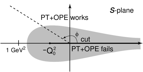
Figure 1: The applicability region of PT and OPE in the complex plane $s$. In the dashed region PT + OPE does not work.

As is well known, in perturbation theory, in the expansion over the powers of inverse $lnQ^{2}$, in the first order in $1/lnQ^{2}$ the running coupling constant $\alpha_{s}(Q^{2})$ has an unphysical pole at some $Q^{2}=Q^{2}_{0}$. If $\beta(a)$ is kept in the denominator in (54), then in $n$-loop approximation $(n>1)$ a branch cut with a singularity $\sim(1-Q^{2}/Q^{2}_{0})^{-1/n}$ appears instead of pole. The position of the singularity is given by

$$ln\frac{Q^{2}_{0}}{\mu^{2}}=-\int\limits^{\infty}_{a(\mu^{2})}\frac{da}{\beta(a)}$$ (56)

Near the singularity the last term in the expansion of $\beta(a)$ dominates and gives the beforementioned behavior. Since the singularity became weaker, one may expect a better convergence of series, which would allow one to go to lower $Q^{2}$.

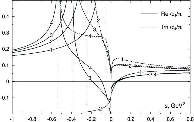
Figure 2: Real and imaginary parts of $\alpha_{\overline{\rm MS}}(s)/\pi$ as an exact numerical solution of RG equation (54) on real axes for different number of loops. The initial condition is chosen $\alpha_{s}=0.355$ at $s=-m_{\tau}^{2}$, $N_{f}=3$. Vertical dotted lines display the position of the unphysical singularity at $s=-Q_{0}^{2}$ for each approximation ($4\to 1$ from left to right).

The real and imaginary parts of $\alpha_{s}(s)/\pi$, obtained as numerical solutions of eq.(54) for various numbers of loops are plotted in Fig.2 as functions of $s=-Q^{2}$. The $\tau$-lepton mass was chosen as normalization point, $\mu^{2}=m^{2}_{\tau}$ and $\alpha_{s}(m^{2}_{\tau})=0.355$ was put in. As is seen from Fig.2, at negative $s$ the perturbation theory converges at $s<-1GeV^{2}$ and in order to have a good precision of the results 4 loops calculations are necessary. At positive $s$, especially for $Im(\alpha_{s}/\pi)$, the convergence of the series is much better. This comes from the fact, that in the chosen integral form of renormalization group equation (54) the expansion over $\pi/ln(Q^{2}/\Lambda^{2})$ is avoided, this expansion being not a small parameter at intermediate $Q^{2}$. (The systematical method of analytical continuation from the spacelike to timelike region with summation of $\pi^{2}$ terms was suggested in [67] and developed in [68]). For instance, in the next to leading order

$$2\pi Im\Pi(s+i0)=1+\frac{1}{\pi\beta_{0}}\Biggl{[}\frac{\pi}{2}-arctg\Biggl{(}\frac{1}{\pi}ln\frac{s}{\Lambda^{2}}\Biggr{)}\Biggr{]}$$ (57)

instead of

$$2\pi Im\Pi(s+i0)=1+\frac{1}{\beta_{0}ln(s/\Lambda^{2})},$$ (58)

which would follow in the case of small $\pi/ln(s/\Lambda^{2})$.

The $\alpha_{s}(Q^{2})$ at $Q^{2}>0$ in low $Q^{2}$ region $(0.8<Q^{2}<5GeV^{2})$ is plotted in Fig.3. (Four loops are accounted, $\alpha_{s}(m^{2}_{\tau})$ is put to be equal to $\alpha_{s}(m^{2}_{\tau})=0.33$. As follows from $\tau$-decay rate $\alpha_{s}(m^{2}_{\tau})=0.352\pm 0.020$ and the value of one standard deviation below the mean one is favoured by low energy sum rules).

Integration over the contour allows one to obviate the dashed region in Fig.1 (except for the vicinity of the positive semiaxis, the contribution of which is suppressed by the factor $(1-\frac{s}{m^{2}_{\tau}})^{2}$ in eq.(51)), i.e. to work in the applicability region of PT+OPE.

Figure 3: $\alpha_{s}(Q^{2})$ normalized at $m_{\tau}^{2}$, $\alpha_{s}(m^{2}_{\tau})=0.33$.

The OPE terms, i.e., power corrections to polarization operator, are given by the formula [1]:

$$\Pi(s)_{nonpert} = \sum_{n\geq 2}{\left<O_{2n}\right>\over(-s)^{n}}\left(1+c_{n}{\alpha_{s}\over\pi}\right)$$ (59)

$$= {\alpha_{s}\over 6\pi\,Q^{4}}\left<0\mid G_{\mu\nu}^{a}G_{\mu\nu}^{a}\mid 0\right>\left(1+{7\over 6}{\alpha_{s}\over\pi}\right)+\frac{4}{Q^{4}}(m_{u}+m_{d})\left<0\mid\bar{q}q\mid 0\right>$$

$$+ {128\over 81\,Q^{6}}\,\pi\alpha_{s}\left<0\mid\bar{q}q\mid 0\right>^{2}_{\mu}\left[1+\left({29\over 24}+{17\over 18}\ln{Q^{2}\over\mu^{2}}\right){\alpha_{s}\over\pi}\right]+{\left<O_{8}\right>\over Q^{8}}$$

($\alpha_{s}$-corrections to the 1-st and 3-d terms in eq.(59) were calculated in [69] and [70], respectively). Contributions of terms proportional to $m^{2}_{u}$, $m^{2}_{d}$ are neglected. When calculating the d=6 term, factorization hypothesis was used. Gluon condensate of dimension $d=6~{}~{}g^{3}\langle 0\mid G^{3}\mid 0\rangle$ (28) does not contribute to polarization operator (59). This is a consequence of the general theorem, proved by Dubovikov and Smilga [71], that in case of self-dual gluonic fields there are no contributions of gluon condensates of dimensions higher than $d=4$ to vector and axial currents polarization operators. Since the vacuum expectation value of $G^{3}$ operator does not vanish for self-dual gluonic fields, this means the vanishing of the coefficient in front of $g^{3}\langle 0\mid G^{3}\mid 0\rangle$ condensate in (59). The same argument refers to dimension 8 gluon operators $g^{4}G^{4}$ with the exception of some of them, like $g^{4}[~{}G^{n}_{\mu\alpha}G^{n}_{\mu\beta}-(1/4)\delta_{\alpha\beta}G^{n}_{\mu\nu}G^{n}_{\mu\nu}~{}]^{2}$, which have zero expectation values in any self-dual field. But the latter are suppressed by a small factor $1/4\pi^{2}$ arising from loop integration in comparison with tree diagram, corresponding to $d=8$ four quark condensate $\langle O_{8}\rangle\sim\langle\bar{q}Gq\cdot\bar{q}q\rangle$ contribution. The contribution from this condensate may be estimated as $\mid\langle O_{8}\rangle\mid<10^{-3}~{}GeV$ [52] (see below, Sec.5.1) and appears to be negligibly small. The $d=8$ two quarks – two gluons operator $O^{\prime}_{8}\sim g^{2}D\bar{q}GGq$ is nonfactorizable, its vacuum mean value is suppressed by $1/N_{c}$ and one may believe, that its contribution to (59) is also small. It can be readily seen that d=4 condensates (up to small $\alpha_{s}$ corrections) give no contribution into the integral over contour eq.(51). $R_{\tau,V+A}$ may be represented as

$$R_{\tau,V+A}=3|V_{ud}|^{2}S_{EW}\left(\,1\,+\,\delta_{em}^{\prime}\,+\,\delta^{(0)}\,+\,\delta^{(6)}_{V+A}\,\right)+\Delta R^{(0)}~{}=~{}3.486\pm 0.016$$ (60)

where $\delta^{\prime}_{em}=(5/12\pi)\alpha_{em}(m^{2}_{\tau})=0.001$ is the electromagnetic correction [72], $\delta^{(6)}_{A+V}=-(3.3\pm 1.1)\cdot 10^{-3}$ is the contribution of d=6 condensate (see below) and $\delta^{(0)}$ is the PT correction. The right-hand part presents the experimental value obtained as a difference between the total probability of hadronic decays $R_{\tau}=3.647\pm 0.014$ [73] and the probability of decays in states with the strangeness $S=-1~{}~{}R_{\tau,s}=0.161\pm 0.007$ [74, 75]. For perturbative correction it follows from eq.(60), that

$$\delta^{(0)}=0.208\pm 0.006$$ (61)

From (61) employing the above described method, the constant $\alpha_{s}(m^{2}_{\tau})$ was found [52]

$$\alpha_{s}(m^{2}_{\tau})=0.352\pm 0.020$$ (62)

The calculation was made with the account of terms $\sim\alpha^{4}_{\tau}$, the theoretical error was assumed to be equal to the last term contribution. May be, the error is underestimated (by $\sim 0.010$), since the theoretical and experimental errors were added in quadratures. The value $\alpha_{s}(m^{2}_{\tau})$ (62) corresponds to:

$$\alpha_{s}(m^{2}_{z})=0.121\pm 0.002$$ (63)

This value is in agreement with recent determination [76] of $\alpha_{s}(m^{2}_{z})$ from the whole set data

$$\alpha_{s}(m^{2}_{z})=0.1182\pm 0.0027$$ (64)

4.2 Instanton corrections

Some nonperturbative features of QCD may be described in the so called instanton gas model (see [77] for extensive review and the collection of related papers in [79]). Namely, one computes the correlators in the $SU(2)$-instanton field embedded in the $SU(3)$ color group. In particular, the 2-point correlator of the vector currents had been computed long ago [80]. Apart from the usual tree-level correlator $\sim\ln{Q^{2}}$ it has a correction which depends on the instanton position and radius $\rho$. In the instanton gas model these parameters are integrated out. The radius is averaged over some concentration $n(\rho)$, for which one or another model is used. Concerning the 2-point correlator of charged axial currents, the only difference from the vector case is that the term with 0-modes must be taken with opposite sign. In coordinate representation the answer can be expressed in terms of elementary functions, see [80]. An attempt to compare the instanton correlators with the ALEPH data in the coordinate space, was made in Ref.[81].

We shall work in momentum space. Here the instanton correction to the spin-$J$ parts $\Pi^{(J)}$ of the correlator (45) can be written in the following form:

$$\Pi^{(1)}_{V,\,{\rm inst}}(q^{2}) = \int_{0}^{\infty}\!d\rho\,n(\rho)\,\left[\,-\,{4\over 3q^{4}}\,+\,\sqrt{\pi}\rho^{4}G^{30}_{13}\left(-\rho^{2}q^{2}\left|{1/2\atop 0,0,-2}\right.\right)\right]$$

$$\Pi^{(0)}_{A,\,{\rm inst}}(q^{2}) = \int_{0}^{\infty}\!d\rho\,n(\rho)\,\left[\,-\,{4\over q^{4}}\,-\,{4\rho^{2}\over q^{2}}\,K_{1}^{2}\!\left(\rho\sqrt{-q^{2}}\right)\right]$$

$$\Pi^{(1)}_{A,\,{\rm inst}}(q^{2}) = \Pi^{(1)}_{V,\,{\rm inst}}(q^{2})-\Pi^{(0)}_{A,\,{\rm inst}}(q^{2})\;,\qquad\Pi^{(0)}_{V,\,{\rm inst}}(q^{2})\,=\,0$$ (65)

Here $K_{1}$ is modified Bessel function, $G_{mn}^{\,p\,q}(z|\ldots)$ is Meijer function. Definitions, properties and approximations of Meijer functions can be found, for instance, in [82]. In particular the function in (65) can be written as the following series:

$$\sqrt{\pi}G^{30}_{13}\left(z\left|{1/2\atop 0,0,-2}\right.\right) = {4\over 3z^{2}}\,-\,{2\over z}\,+\,{1\over 2\sqrt{\pi}}\,\sum_{k=0}^{\infty}\,z^{k}{\Gamma(k+1/2)\over\Gamma^{2}(k+1)\,\Gamma(k+3)}$$ (66)

$$\times \Bigl{\{}\,\left[\,\ln{z}\,+\,\psi(k+1/2)\,-\,2\,\psi(k+1)\,-\,\psi(k+3)\,\right]^{2}$$

$$+ \,\psi^{\prime}(k+1/2)\,-\,2\,\psi^{\prime}(k+1)\,-\,\psi^{\prime}(k+3)\,\Bigr{\}}$$

where $\psi(z)=\Gamma^{\prime}(z)/\Gamma(z)$. For large $|z|$ one can obtain its approximation by the saddle-point method:

$$G^{30}_{13}\left(z\left|{1/2\atop 0,0,-2}\right.\right)\approx\sqrt{\pi}z^{-3/2}e^{-2\sqrt{z}}\;,\qquad|z|\gg 1$$ (67)

The formulae (65) should be treated in the following way. One adds $\Pi_{\rm inst}$ to usual polarization operator with perturbative and OPE terms. But the terms $\sim 1/q^{4}$ must be absorbed by the operator $O_{4}$ in Eq.(65), since the gluonic condensate $\bigl{<}G^{2}\bigr{>}$ is averaged over all field configurations, including the instanton one. Notice negative sign before $1/q^{4}$ in Eq.(64). This happens because the negative contribution of the quark condensate $\bigl{<}m\bar{q}q\bigr{>}$ in the instanton field exceeds positive contribution of the gluonic condensate $\bigl{<}G^{2}\bigr{>}$. In real world $\bigl{<}m\bar{q}q\bigr{>}$ is negligible.

The correlators (65) possess appropriate analytical properties, they have a cut along positive real axes:

$${\rm Im}\,\Pi^{(1)}_{V,\,{\rm inst}}(q^{2}+i0)=\int_{0}^{\infty}\!d\rho\,n(\rho)\,\pi^{3/2}\rho^{4}G^{20}_{13}\left(\rho^{2}q^{2}\left|{1/2\atop 0,0,-2}\right.\right)$$ (68)

$${\rm Im}\,\Pi^{(0)}_{A,\,{\rm inst}}(q^{2}+i0)=-\,\int_{0}^{\infty}\!d\rho\,n(\rho)\,{2\pi^{2}\rho^{2}\over q^{2}}J_{1}\!\left(\rho\sqrt{q^{2}}\right)N_{1}\!\left(\rho\sqrt{q^{2}}\right)$$ (69)

We shall consider below the instanton gas model. It is a model with fixed instanton radius

$$n(\rho)\,=\,n_{0}\,\delta(\rho-\rho_{0})$$ (70)

In [77] it was estimated:

$$\rho_{0}\,\approx\,1/3\,{\rm fm}\,\approx\,1.5-2.0\,{\rm GeV}^{-1}\;,\qquad n_{0}\,\approx\,1\,{\rm fm}^{-4}\,\approx(1.0-\,1.5)\times 10^{-3}\,{\rm GeV}^{4}$$ (71)

In fact, the instanton liquid model, with the account of instanton self-interaction was mainly considered in [77], but the arguments, from which the estimations (71) follow, refer also to the instanton gas model. In this case, the value of $n_{0}$ (71) should be considered as an upper limit (see also [78]).

Now we consider the instanton contribution to the $\tau$-decay branching ratio. Since the instanton correlator (65) has $1/q^{2}$ singular term in the expansion near 0 (see Eq. (66)), the integrals must be taken over the circle, as in (51). In the instanton model the function $a_{0}(s)$ differs from experimental $\delta$-function, which gives small correction. So we shall ignore the last term in (48) and consider the integral with $\Pi_{V+A}^{(1)}+\Pi_{A}^{(0)}$ in (51). The instanton correction to the $\tau$-decay branching ratio can be brought to the following form:

$$\delta_{\rm inst}\,=\,-\,48\,\pi^{5/2}\int_{0}^{\infty}\!d\rho\,n(\rho)\,\rho^{4}\,G^{20}_{13}\left(\rho^{2}m_{\tau}^{2}\left|{1/2\atop 0,-1,-4}\right.\right)\approx\,{48\pi^{2}n_{0}\over\rho_{0}^{2}m_{\tau}^{6}}\,\sin{(2\rho_{0}m_{\tau})}$$ (72)

Since the parameters (71) are determined quite approximately, we may explore the dependence of $\delta_{\rm inst}$ on them. The $\delta_{\rm inst}$ versus $\rho_{0}$ for fixed $n_{0}=1.5\cdot 10^{-3}GeV^{4}$ is shown in Fig.4.

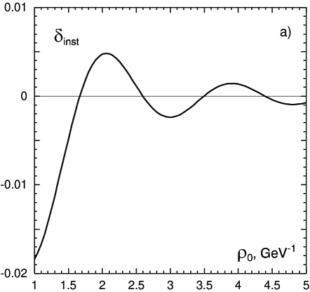
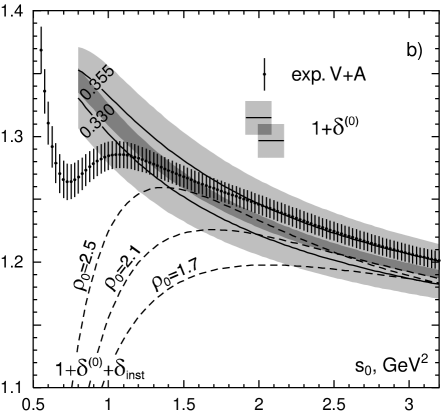
Figure 4: The instanton correction to the $\tau$ decay ratio versus $\rho_{0}$ (a) and ”versus $\tau$ mass” (b) for $n_{0}=1.5\times 10^{-3}\,{\rm GeV}^{4}$. The thin solid lines in Fig.4b are the values of $1+\delta^{(0)}(s_{0})$, where $\delta^{(0)}(s_{0})$ are perturbative corrections, calculated as described in Sec.4.1. The upper curve corresponds to $\alpha_{s}(m^{2}_{\tau})=0.355$, the lower one – to $\alpha_{s}(m^{2}_{\tau})=0.330$. The shadowed regions represent the uncertainties in perturbative calculations, the dark shadowed band is their overlop. The dashed lines are $1+\delta^{(0)}(s)+\delta_{inst},\delta^{(0)}(s)$ corresponds to $\alpha_{s}(m^{2}_{\tau})=0.330$.

As seen from Fig.4a the instanton correction to hadronic $\tau$-decay is extremely small except for unreliably low value of the instanton radius $\rho_{0}<1.5\,{\rm GeV}^{-1}$. At the favorable value [77] $\rho_{0}=1.7\,{\rm GeV}^{-1}$ the instanton correction to $R_{\tau}$ is almost exactly zero. This fact confirms the calculations of $\alpha_{s}(m_{\tau}^{2})$ (Sec. 4.1), where the instanton corrections were not taken into account.

Eq.(72) can be used in another way. Namely, the $\tau$ mass can be considered as free parameter $s_{0}$. The dependence of the fractional corrections $\delta^{(0)}$ and $\delta^{(0)}_{0.330}+\delta_{\rm inst}$ on $s_{0}$ is shown in Fig.4b. The result strongly depends on the instanton radius and rather essentially on the density $n_{0}$. For $\rho_{0}=1.7\,{\rm GeV}^{-1}$ and $n_{0}=1\,{\rm fm}^{-4}$, the instanton curve is outside the errors already at $s_{0}\sim 2\,{\rm GeV}^{2}$, where the perturbation theory is expected to work.

We came to the conclusion, that in case of variable $\tau$ mass the instanton contribution becomes large at $s_{0}<2GeV^{2}$. That means, that $R_{\tau,V+A}(s_{0})$ given by (51) cannot be represented by PT+OPE at $s_{0}<2GeV^{2}$ and the results, obtained in this way are not reliable.

4.3 Comparison with other approaches

There are many calculations of $\alpha_{s}(m^{2}_{\tau})$ from the total $\tau$-decay rate, using the same idea, which was used above – the countour improved fixed order perturbation theory [53, 55, 57]-[59, 73]. (For more recent ones, see [23, 54].) The results of these calculations coincide with presented above in the limit of errors and give $\alpha_{s}(m^{2}_{\tau})=0.33-0.35$. From these values by using renormalization group one can find $\alpha_{s}(m^{2}_{z})=0.118-0.121$ in agreement with $\alpha_{s}(m^{2}_{z})$ determinations from other processes (see [13],[76]).

Till now only one renormalization scheme was considered – the $\overline{MS}$ scheme. In BLM renormalization scheme [83], which have some advantages from the point of view of perturbative pomeron theory [84], the result is $\alpha_{s}(m^{2}_{\tau})=0.621\pm 0.008$ [85], corresponding in the framework of BLM scheme to the same value of $\alpha_{s}(m^{2}_{z})=0.117-0.122$. At low scales, however, the $\alpha_{s}(Q^{2})$ behavior is essentially different from that, presented in Fig.3.

Few words about $\alpha_{s}$ calculations in analytical QCD (see [86] and references herein). According to this theory the coupling constant $\alpha_{s}(Q^{2})$ is calculated by renormalization group in the spacelike region $Q^{2}>0$. Then, by analytical continuation to $s=-Q^{2}>0$ $Im\alpha_{s}(s)$ was found on the right semiaxes. It was assumed, that $\alpha_{s}(s)$ is an analytical function in the complex $s$-plane with a cut along the right semiaxes $0\leq s\leq\infty$. The analytical $\alpha_{s}(s)_{an}$ is then defined in the whole $s$-plane by dispersion relation. Such $\alpha_{s}(s)_{an}$ has no unphysical singularities. Let us calculate $\alpha_{s}(m^{2}_{\tau})_{an}$ using the same experimental data as before, i.e. $\delta^{(0)}$ given by Eq.(61). In the analytical QCD the countour integral (51) is equal to the integral of $Im\Pi(s)$ over real positive axes. (In the previous calculation the integral was running from $s=-Q^{2}_{0}$ to $m^{2}_{\tau}$.) Qualitatively, it leads to much smaller $R_{\tau}$ in the analytical QCD than in the conventional approach with the same $\alpha_{s}(m^{2}_{\tau})$, or vice versa, it is necessary to have much larger $\alpha_{s}(m^{2}_{\tau})_{an}$ in order to get experimental $R_{\tau}$. The calculation of integral (51) with $\Pi(s)$ expressed through $\alpha_{s}(s)_{anal}$, shows that experimental $R_{\tau}$ results in $\alpha_{s}(m^{2}_{z})=0.141\pm 0.004$ in contradiction with other data. (In [87] an attempt was made to get an agreement of analytical QCD with common value of $\alpha_{s}(m^{2}_{z})$. For this goal the constituent quark model with specific quark-antiquark potential was used in the domain of low and intermediate $s$. Evidently, such approach cannot be considered as $\alpha_{s}$ determination in QCD: in this approach QCD is modified on large circle in complex plane of the radius $\mid s\mid=m^{2}_{\tau}$ in contradiction with the basic assumption of $\alpha_{s}$ calculation from hadronic $\tau$-decay rate.)

5 Determination of condensates from spectral functions of $\tau$-decay

5.1 Determination of quark condensate from $V-A$ spectral function

In order to determine the quark condensate from $\tau$-decay data it is convenient to consider the difference $V-A$ of polarization operators $\Pi^{(1)}_{V}-\Pi^{(1)}_{A}$, where the contribution of perturbative terms is absent. $\Pi^{(1)}_{V}(s)-\Pi^{(1)}_{A}(s)$ is represented by OPE:

$$\Pi^{(1)}_{V}(s)-\Pi^{(1)}_{A}(s)=\sum_{D\geq 4}\frac{O^{V-A}_{D}}{(-s)^{D/2}}\Biggl{(}1+c_{D}\frac{\alpha_{s}(s)}{\pi}\Biggr{)}$$ (73)

The gluonic condensates contribution drops out in the $V-A$ difference and only the following condensates up to D=10 remain

$$O^{V-A}_{4}=2\,(m_{u}+m_{d})\,\langle 0\mid\bar{q}q\mid 0\rangle\;=\;-\,f_{\pi}^{2}m_{\pi}^{2}~{}[1]$$ (74)

$$O^{V-A}_{6}=2\pi\alpha_{s}\left<0\mid(\bar{u}\gamma_{\mu}\lambda^{a}d)(\bar{d}\gamma_{\mu}\lambda^{a}u)-(\bar{u}\gamma_{5}\gamma_{\mu}\lambda^{a}d)(\bar{d}\gamma_{5}\gamma_{\mu}\lambda^{a}u)\mid 0\right>=$$

$$=-\,{64\pi\alpha_{s}\over 9}\langle 0\mid\bar{q}q\mid 0\rangle^{2}~{}[1]$$ (75)

$$O^{V-A}_{8}=-8\pi\alpha_{s}\,m_{0}^{2}\langle 0\mid\bar{q}q\mid 0\rangle^{2}~{},~{}\cite[cite]{[\@@bibref{}{Dubovikov,41}{}{}]}~{}$$ (76)

$$O^{V-A}_{10}=-\frac{8}{9}\pi\alpha_{s}\langle 0\mid\bar{q}q\mid 0\rangle^{2}\Biggl{[}\frac{50}{9}m^{4}_{0}+32\pi^{2}\langle 0\mid\frac{\alpha_{s}}{\pi}G^{2}\mid 0\rangle\Biggr{]}~{}\cite[cite]{[\@@bibref{}{76}{}{}]}$$ (77)

where $m^{2}_{0}$ is determined in eq.(24). In the right-hand of (75),(76),(77) the factorization hypothesis was used. For $O_{6}$ operator it is expected [1], that the accuracy of factorization hypothesis is of order $1/N^{2}_{c}\sim 10\%$, where $N_{c}=3$ is the number of colours. For operators of dimensions $d\geq 8$ the factorization procedure is not unique. (But, as a rule, the arising differences are not very large – for $d=8$ operator entering eq.(73) it is about 20%). The accuracy of factorization hypothesis becomes worse with increasing of operator dimensions: for $O^{V-A}_{8}$, it is worse, than for $O^{V-A}_{6}$ and for $O^{V-A}_{10}$ it is worse than for $O^{V-A}_{8}$.

Operators $O_{4}$ and $O_{6}$ have approximately zero anomalous dimensions, the $O_{8}$ anomalous dimension is equal to – 11/27. Calculations of the coefficients in front of $\alpha_{s}$ in eq.(73) gave $c_{4}=4/3$ [90] and $c_{6}=89/48$ [91]. (For $O_{4}$ the $\alpha^{2}_{s}$ correction is known [90]: $(59/6)(\alpha_{s}/\pi)^{2})$.) The $\alpha_{s}$ corrections to $O^{V-A}_{8}$ are unknown – they are included into the not certainly known value of $m^{2}_{0}$, $\alpha_{s}$ corrections to $O_{10}$ are unknown also. (In this Section indeces $V-A$ will be omitted and $O_{D}$ will mean condensates with $\alpha_{s}$ corrections included.)

Our aim is to compare the OPE theoretical predictions with the experimental data on $V-A$ structure functions measured in $\tau$-decay and with the help of such comparison to determine the magnitude of the most important condensate $O_{6}$. The condensate $O_{4}$ is small and is known with a good accuracy:

$$O_{4}=-0.5\cdot 10^{-3}~{}GeV^{4}$$ (78)

We put $m^{2}_{0}=0.8GeV^{2}$ and in the analysis of the data the values of the condensates $O_{8}$ and $O_{10}$ are taken to be equal to

$$O_{8}=-2.8\cdot 10^{-3}~{}GeV^{8}$$ (79)

$$O_{10}=-2.6\cdot 10^{-3}~{}GeV^{10}$$ (80)

and their $Q^{2}$-dependence, arising from anomalous dimensions is neglected.

In  the  calculation  of  numerical  values  (78),(79) it  was  assumed,  that  $a_{\bar{q}q}(1~{}GeV^{2})\equiv$
$\equiv-(2\pi)^{2}\langle 0\mid\bar{q}q\mid 0\rangle_{1GeV}=0.65~{}GeV^{3}$, $\langle 0\mid(\alpha_{s}/\pi)G^{2}\mid 0\rangle=0.005~{}GeV^{4}$ – see below, eq.’s (87),(117).

As was shown in [51] the dimension $d=8$ four-quark operators for vector and axial currents are of opposite sign and equal in absolute values up to terms of order $1/N^{2}_{c}$: $O^{V}_{8}=-O^{A}_{8}(1+O(N^{-2}_{c}))$. (The exact value of $N^{-2}_{c}$ correction is uncertain – it depends on factorization procedure.) So, for $O^{V+A}_{8}$ we have from (79) the estimation: $\mid O^{V+A}_{8}\mid<10^{-3}~{}GeV^{8}$, which was used in calculation $\Pi(s)_{nonpert}$, Eq.(59).

For $\Pi^{(1)}_{V}(s)-\Pi^{(1)}_{A}(s)$ substractionless dispersion relation is valid:

$$\Pi^{(1)}_{V}(s)-\Pi^{(1)}_{A}(s)\,=\,{1\over 2\pi^{2}}\int_{0}^{\infty}{v_{1}(t)-a_{1}(t)\over t-s}\,dt\,+\,{f_{\pi}^{2}\over s}$$ (81)

(The last term in the right-hand part is the kinematic pole contribution). The experimental data for $v_{1}(s)-a_{1}(s)$ are presented in Fig.5

Figure 5: The measured difference $v_{1}(s)-a_{1}(s)$. Figures from [48] and [49], reproduced in [51].

In order to improve the convergence of OPE series as well as to suppress the contribution of large $s$ domain in dispersion integral use the Borel transformation. Put $s=s_{0}e^{i\phi}$ ($\phi=0$ on the upper edge of the cut) and make the Borel transformation in $s_{0}$. As a result, we get the following sum rules for the real and imaginary parts of (81):

$$\int_{0}^{\infty}\exp{\!\left({s\over M^{2}}\cos{\phi}\right)}\cos{\!\left({s\over M^{2}}\sin{\phi}\right)}(v_{1}-a_{1})(s)\,{ds\over 2\pi^{2}}\,=\,f_{\pi}^{2}+\,\sum_{k=1}^{\infty}(-1)^{k}{\cos{(k\phi)}\,O_{2k+2}\over k!\,M^{2k}}$$ (82)

$$\int_{0}^{\infty}\exp{\!\left({s\over M^{2}}\cos{\phi}\right)}\,\sin{\!\left({s\over M^{2}}\sin{\phi}\right)}(v_{1}-a_{1})(s)\,{ds\over 2\pi^{2}M^{2}}\,=\,\sum_{k=1}^{\infty}(-1)^{k}{\sin{(k\phi)}\,O_{2k+2}\over k!\,M^{2k+2}}$$ (83)

The use of the Borel transformation along the rays in the complex plane has a number of advantages. The exponent index is negative at $\pi/2<\phi<3\pi/2$. Choose $\phi$ in the region $\pi/2<\phi<\pi$. In this region, on one hand, the shadowed area in Fig. 1 in the integrals (82),(83) is touched to a less degree, and on the other hand, the contribution of large $s$, particularly, $s>m^{2}_{\tau}$ , where experimental data are absent, is exponentially suppressed. At definite values of $\phi$ the contribution of some condensates vanishes, what may be also used. In particular, the condensate $O_{8}$ does not contribute to (82) at $\phi=5\pi/6$ and to (83) at $\phi=2\pi/3$, while the contribution of $O_{6}$ to (82) vanishes at $\phi=3\pi/4$. Finally, a well known advantage of the Borel sum rules is factorial suppression of higher dimension terms of OPE. Figs.6,7 present the results of the calculations of the left-hand parts of eqs.(82),(83) on the basis of the ALEPH [48] experimental data comparing with OPE predictions – the right-hand part of these equations.

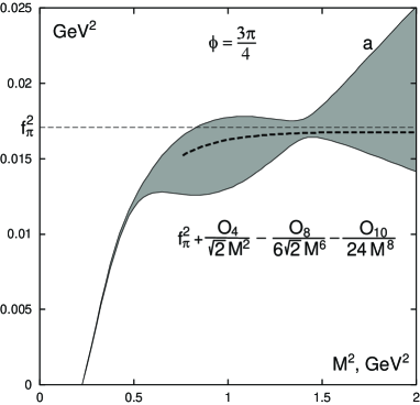
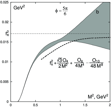
Figure 6: Eq.(82): the left-hand part is obtained basing on the experimental data, the shaded region corresponds to experimental errors; the right-hand part – the theoretical one – is represented by the dotted curve, numerical values of condensates $O_{4},O_{8},O_{10},O_{6}$ are taken according to (78),(79),(80),(84); a) $\phi=3\pi/4$,  b) $\phi=5\pi/6$.

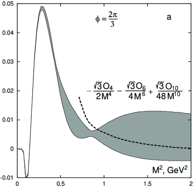
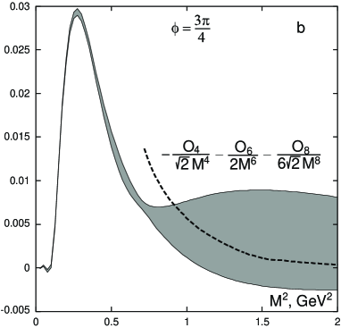
Figure 7: The same for eq.(83): a) $\phi=2\pi/3$,   b) $\phi=3\pi/4$.

When comparing the theoretical curves with experimental data it must be taken in mind, that the value of $f_{\pi}$, which in the figures was taken to be equal to experimental one $f_{\pi}=130.7MeV$, in fact has a theoretical uncertainty of the order $(\Delta f^{2}_{\pi}/f^{2}_{\pi})_{theor}\sim m^{2}_{\pi}/m^{2}_{\rho}$, where $m_{\rho}$ is characteristic hadronic scale (say, $\rho$-meson mass). This uncertainty is caused by chiral symmetry violation in QCD. Particularly, the account of this uncertainty may lead to a better agreement of theoretical curve with the data in Fig.6b. The calculation of instanton contributions (Eq.(65)), shows, that in all considered above cases they are less than $0.5\cdot 10^{-3}$ at $M^{2}>0.8~{}GeV^{2}$, i.e. are well below the errors. (In some cases they improve the agreement with the data.) The best fit of the data (the dashed curves at Fig.’s 6,7) was achieved at the value

$$O_{6}=-4.4\cdot 10^{-3}~{}GeV^{6}$$ (84)

It follows from (84) after separating $\alpha_{s}$ correction $[1+(89/48)\alpha_{s}/\pi)=1.33]$:

$$\alpha_{s}\langle 0\mid\bar{q}q\mid 0\rangle^{2}=1.5\cdot 10^{-4}~{}GeV^{6}$$ (85)

The error may be estimated as 30%. The value (85) in the limit of errors agrees with previous estimation [51]. The contribution of dimension 10 is negligible in all cases at $M^{2}\geq 1~{}GeV^{2}$. It is worth mentioning that the theory, i.e. the OPE agrees with the data at $M^{2}>0.8~{}GeV^{2}$. The good agreement of the theoretical curves with the data confirms the chosen value of $O_{8}$ (78) and, therefore, the use of factorization hypothesis. From (84), with the use of $\alpha_{s}(1GeV^{2})=0.55$ (see Fig.3) the value of quark condensate at 1 GeV can be found

$$\langle 0|qq|0\rangle_{1~{}GeV}=-1.65\cdot 10^{-2}~{}GeV^{3}=-(254~{}MeV)^{3}$$ (86)

and the convenient parameter is

$$a_{\bar{q}q}(1~{}GeV^{2})\equiv-(2\pi)^{2}\langle 0|\bar{q}q|0\rangle_{1~{}GeV}=0.65~{}GeV^{3}$$ (87)

The magnitude of quark condensate (86) is close to that which follows from the Gell-Mann-Oakes-Renner relation (eq.(22)).

In the last years there were many attempts [53],[92]-[98] to determine quark condensates using V-A spectral functions measured in $\tau$-decay. Unlike the approach presented above, where the polarization operator analytical properties were exploited in the whole complex $q^{2}$-plane, what allowed one to separate the contribution of operators of different dimensions, the authors of [53],[92]-[98] considered the finite energy sum rules - FESR (or integrals over contours) with chosen weight functions. In [92, 94] the $N_{c}\to\infty$ limit was used. In [93, 94, 95, 98] an attempt was made to find higher dimension condensates (up to 18 in [87], up to 16 in [93, 94] and up to 12 in [95]). Determination of higher dimension condensates requires fine tunning of the upper limit of integration in FESR. If the upper limit of integration $s_{0}$ in FESR is below $2~{}GeV^{2}$ (e.g., such an upper limit, $s_{0}=1.47~{}GeV$ was chosen in [98]), then instanton-like corrections, not given by OPE are of importance. (See Sec.4.2). The same remark refers to the case of weight factors singular at $s=0$, like $s^{-l}$, $l>0$ [53], when there is an enhancement of the contribution of low $s$, where OPE breaks down. Taking in mind these remarks, we have a satisfactory agreement of the values of condensate (84), presented above, with those found in [53, 94, 98].

5.2 Determination of condensates from $V+A$ and $V$ structure functions of $\tau$-decay

Let us turn now to study the $V+A$ correlator in the domain of low $Q^{2}$, where the OPE terms play a much more essential role, than in the determination of $R_{\tau}$. A general remark is in order here. As was discussed in Ref.[28] and stressed recently by Shifman [29], the condensates cannot be defined in rigorous way, because there is some arbitrariness in the separation of their contributions from perturbative part. Usually [28, 29] they are defined by introduction of some normalization point $\mu^{2}$ with the magnitude of few $\Lambda^{2}_{QCD}$. The integration over momenta in the domain below $\mu^{2}$ is addressed to condensates, above $\mu^{2}$ – to perturbation theory. In such formulation the condensates are $\mu$-dependent $\left<O_{D}\right>=\left<O_{D}\right>_{\mu}$ and, strictly speaking, they also depend on the way how the infrared cut-off $\mu^{2}$ is introduced. The problem becomes more severe when the perturbative expansion is performed up to higher order terms and the calculation pretends on high precision. Mention, that this remark does not refer to chirality violating condensates, because perturbative terms do not contribute to chirality violating structures in the limit of massless quarks. For this reason, in principle, chirality violating condensates, e.g. $\bigl{<}0|\bar{q}q|0\bigr{>}$, can be determined with higher precision, than chirality conserving ones. Here I use the definition of condensates, which can be called $n$-loop condensates. As was formulated in Chapt.4, we treat the renormalization group equation (54) and the equation for polarization operator (55) in $n$-loop approximation as exact ones; the expansion in inverse logarithms is not performed. Specific values of condensates are referred to such procedure. Of course, their numerical values depend on the accounted number of loops; that is why the condensates, defined in this way, are called $n$-loop condensates.

Consider the polarization operator $\Pi=\Pi_{V+A}^{(1)}+\Pi_{A}^{(0)}$, defined in (50) and its imaginary part

$$\omega(s)\,=\,v_{1}(s)\,+\,a_{1}(s)\,+\,a_{0}(s)\,=\,2\pi\,{\rm Im}\,\Pi(s+i0)$$ (88)

In parton model $\omega(s)\to 1$ at $s\to\infty$. Any sum rule can be written in the following form:

$$\int_{0}^{s_{0}}f(s)\,\omega_{\rm exp}(s)\,ds\,=\,i\pi\oint f(s)\,\Pi_{\rm theor}(s)\,ds$$ (89)

where $f(s)$ is some analytical in the integration region function. In what follows we use $\omega_{\rm exp}(s)$, obtained from $\tau$-decay invariant mass spectra published in [48] for $0<s<m_{\tau}^{2}$. The experimental error of the integral (89) is computed as the double integral with the covariance matrix $\overline{\omega(s)\omega(s^{\prime})}-\overline{\omega}(s)\overline{\omega}(s^{\prime})$, which also can be obtained from the data available in Ref.[48]. In the theoretical integral in (89) the contour goes from $s_{0}+i0$ to $s_{0}-i0$ counterclockwise around all poles and cuts of theoretical correlator $\Pi(s)$. Because of Cauchy theorem the unphysical cut must be inside the integration contour.

The choice of the function $f(s)$ in Eq.(89) is actually a matter of taste. At first let us consider usual Borel transformation:

$$B_{\rm exp}(M^{2})\,=\,\int_{0}^{m_{\tau}^{2}}e^{-s/M^{2}}\omega_{\rm exp}(s)\,{ds\over M^{2}}\,=\,B_{\rm pt}(M^{2})\,+\,2\pi^{2}\sum_{n}{\bigl{<}O_{2n}\bigr{>}\over(n-1)!\,M^{2n}}$$ (90)

We separated out the purely perturbative contribution $B_{\rm pt}$, which is computed numerically according to (89) and Eqs.(52)-(55). Remind that Borel transformation improves the convergence of OPE series because of the factors $1/(n-1)!$ in front of operators and suppresses the contribution of high-energy tail, where the experimental error is large. But it does not suppress the unphysical perturbative cut, the main source of the error in this approach, even increase it since $e^{-s/M^{2}}>1$ for $s<0$. So the perturbative part $B_{\rm pt}(M^{2})$ can be reliably calculated only for $M^{2}\mathrel{\mathchoice{\lower 3.6pt\vbox{\halign{$\mathsurround=0pt\displaystyle\hfil#\hfil$\cr>\crcr\sim\crcr}}}{\lower 3.6pt\vbox{\halign{$\mathsurround=0pt\textstyle\hfil#\hfil$\cr>\crcr\sim\crcr}}}{\lower 3.6pt\vbox{\halign{$\mathsurround=0pt\scriptstyle\hfil#\hfil$\cr>\crcr\sim\crcr}}}{\lower 3.6pt\vbox{\halign{$\mathsurround=0pt\scriptscriptstyle\hfil#\hfil$\cr>\crcr\sim\crcr}}}}0.8-1\,{\rm GeV}^{2}$ and higher; below this value the influence of the unphysical cut is out of control.

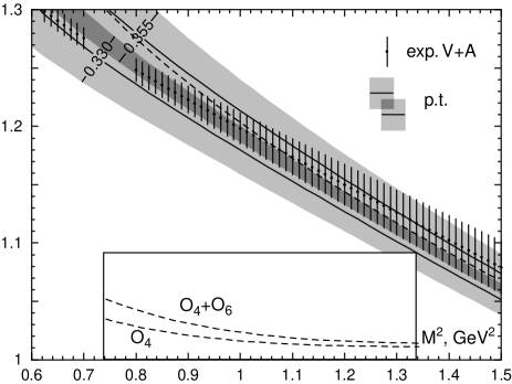
Figure 8: The results of the Borel transformation of $V+A$ correlator for two values $\alpha_{s}(m^{2}_{\tau})=0.355$ and $\alpha_{s}(m^{2}_{\tau})=0.330$. The widths of the bands correspond to PT errors, dots with dashed errors – experimental data. The dashed curve is the sum of the perturbative contribution at $\alpha_{s}(m^{2}_{\tau})=0.330$ and $O_{4}$, (Eq.’s (59),(92)) and $O_{6}$ (Eq.’s (59),(85)) condensate contributions.

Both $B_{\rm exp}$ and $B_{\rm pt}$ in 4-loop approximation for $\alpha_{s}(m_{\tau}^{2})=0.355$ and $0.330$ are shown in Fig.8. The shaded areas display the theoretical error. They are taken equal to the contribution of the last term in the perturbative Adler function expansion $K_{4}a^{4}$ (52).

The contribution of the $O_{8}$ operator is of order $O^{V-A}_{8}/N^{2}_{c}$ and negligible [51]. (In fact, it depends on the factorization procedure and uncertain for this reason). The contributions of $D=4$ and $D=6$ operators are positive [see (59)]. So, the theoretical perturbative curve must go below the experimental points. The result shown in Fig.8 is in the favour of the lower value of the QCD coupling constant $\alpha_{s}(m^{2}_{\tau})=0.330$ (or, may be, $\alpha_{s}(m^{2}_{\tau})=0.340$). As is seen from Fig.8, the theoretical curve (perturbative at $\alpha_{s}(m^{2}_{\tau})=0.330$ plus OPE terms) is in agreement with experiment at $M^{2}\geq 0.9~{}GeV^{2}$.

In order to separate the contribution of gluon condensate let us perform the Borel transformation along the rays in the complex $s$-plane in the same way, as it was done in Sec.5.1. The real part of the Borel transform at $\phi=5\pi/6$ does not contain $d=6$ operator.

$$ReB_{exp}(M^{2}e^{i5\pi/6})=ReB_{pt}(M^{2}e^{i5\pi/6})+\pi^{2}\frac{\langle O_{4}\rangle}{M^{4}}$$ (91)

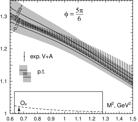
Figure 9: Real part of the Borel transform (91) along the ray at the angle $\phi=5\pi/6$ to the real axes. The dashed line corresponds to the gluonic condensate given by the central value of (92).

The results are shown in Fig.9. If we accept the lower value of $\alpha_{s}(m^{2}_{\tau})$, we get the following restriction on the value of gluon condensate:

$$\left<{\alpha_{s}\over\pi}\,G_{\mu\nu}^{a}G_{\mu\nu}^{a}\right>\,=\,0.006\pm 0.012\,{\rm GeV}^{4}\;,\qquad\alpha_{s}(m_{\tau}^{2})=0.330\quad{\rm and}\quad M^{2}>0.8\,{\rm GeV}^{2}$$ (92)

The theoretical and experimental errors are added in quadratures in Eq.(92).

Turn now to analysis of the vector correlator (the vector spectral function was published by ALEPH in [99]). In principle this cannot give any new information in comparison with $V-A$ and $V+A$ cases. However the analysis of the vector current correlator is important since it can also be performed with the experimental data on $e^{+}e^{-}$ annihilation. The imaginary part of the electromagnetic current correlator, measured there, is related to the charged current correlator (45) by the isotopic symmetry. The statistical error in $e^{+}e^{-}$ experiments is less than in $\tau$-decays because of significantly larger number of events. So it would be interesting to perform similar analysis with $e^{+}e^{-}$ data, which is a matter for separate research.

At first we consider usual Borel transformation for vector current correlator, since it was originally applied in [100] for the sum rule analysis. It is defined as (89) with the experimental spectral function $\omega_{\rm exp}=2v_{1}$ instead of $v_{1}+a_{1}+a_{0}$ (the normalization is $v_{1}(s)\to 1/2$ at $s\to\infty$ in parton model). Respectively, in the r.h.s. one should take the vector operators $2O^{V}=O^{V+A}+O^{V-A}$. The numerical results are shown in Fig.10. The perturbative theoretical curves are the same as in Fig.8 with $V+A$ correlator. The dashed lines display the contributions of the gluonic condensate given by Eq.(92), $2O_{6}^{V}=-3.5\times 10^{-3}\,{\rm GeV}^{6}$ and $2O_{8}^{V}=O_{8}^{V-A}=-2.8\times 10^{-3}\,{\rm GeV}^{8}$ added to the $\alpha_{s}(m^{2}_{\tau})=0.330$-perturbative curve. The contribution of each condensate is shown in the box below. Notice, that for such condensate values the total OPE contribution is small, since positive $O_{4}$ compensate negative $O_{6}$ and $O_{8}$. The agreement is observed for $M^{2}>0.8\,{\rm GeV}^{2}$.

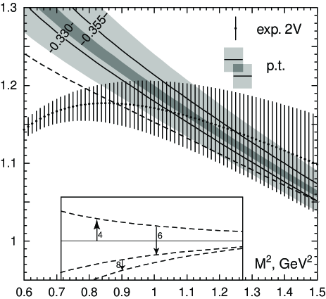
Figure 10: Borel transformation for vector currents.

The Borel transformations along the rays in the complex plane results in the same conclusion; at $M^{2}>0.8-0.9~{}GeV^{2}$ the agreement with experiment at 2% level is achieved at $\alpha_{s}(m^{2}_{\tau})=0.33-0.34$ and at the values of quark and gluon condensates given by (84) and (92). There is some discrepancy in the vector spectral function obtained in $\tau$-decay and in $e^{+}e^{-}$ annihilation (see [54], [101] and references herein): the $e^{+}e^{-}$ data are below $\tau$-decay ones by 5-10% in the interval $s=0.6-0.8~{}GeV^{2}$. The substitution of $e^{+}e^{-}$ data instead of $\tau$-decay data in the sum rule presented in Fig.10 does not spoil the agreement of the theory with experiment in the limit of errors.

A few words about instanton contributions. They can be calculated in the same way, as in the case of $V-A$ correlators. At the chosen values of instanton gas parameters instanton contributions are small, less than $0.5\cdot 10^{-3}$ at $M^{2}>0.8~{}GeV^{2}$ and do not spoil the agreement of the theory with experiment.

6 Determination of quark condensate from QCD sum rules for baryon masses

Since in QCD with massless quarks the baryon masses arise due to spontaneous violation of chiral symmetry and in a good approximation, the proton mass (as well as $\Delta$-isobar) can be expressed through quark condensate [32], the QCD sum rules for baryon masses are a suitable tool for determination of quark condensate assuming that baryon masses are known. The sum rules can be derived by considering the polarization operator

$$\Pi(p)=i~{}\int~{}d^{4}xe^{ipx}\langle 0|T\{\eta(x),\bar{\eta}(0)\}|0\rangle$$ (93)

where $\eta(x)$ is the quark current with baryon quantum numbers. In case of proton the most suitable current is [32, 102].

$$\eta(x)=\varepsilon^{abc}(u^{a}C\gamma_{\mu}u^{b})\gamma_{5}\gamma_{\mu}d^{c}$$ (94)

where $u^{a}$, $d^{c}$ – are $u$ and $d$ quark fields, $a,b,c$ are colour indeces, $C$ is the charge conjugation matrix. After Borel transformation the sum rules for proton mass have the form [32, 37, 44]

$$M^{6}E_{2}(s_{0}/M^{2})L^{-4/9}\Biggl{[}1+\Biggl{(}\frac{53}{12}+\gamma_{E})\frac{\alpha_{s}(M^{2})}{\pi}\Biggr{]}+\frac{1}{4}M^{4}bE_{0}(s_{0}/M^{2})L^{-4/9}+$$

$$+\frac{4}{3}a^{2}_{\bar{q}q}\Biggl{[}1+f(M^{2})\frac{\alpha_{s}(M^{2})}{\pi}\Biggr{]}-\frac{1}{3}a^{2}_{\bar{q}q}\frac{m^{2}_{0}}{M^{2}}=\bar{\lambda}^{2}_{p}e^{-m^{2}/M^{2}}$$ (95)

$$2a_{\bar{q}q}M^{4}E_{1}(s_{0}/M^{2})\Biggl{[}1+\frac{3}{2}~{}\frac{\alpha_{s}(M^{2})}{\pi}\Biggr{]}+\frac{272}{81}~{}\frac{\alpha_{s}(M^{2})}{\pi}~{}\frac{a^{3}_{\bar{q}q}}{M^{2}}-\frac{1}{12}a_{\bar{q}q}b=m\bar{\lambda}^{2}_{p}e^{-m^{2}/M^{2}}$$ (96)

Here $M$ is the Borel parameter, $m$ is the nucleon mass, $a_{\bar{q}q}$ is given by (87), $\gamma_{E}=0.577$.

$$b=(2\pi)^{2}\langle 0|\frac{\alpha_{s}}{\pi}~{}G^{2}|0\rangle$$ (97)

$$E_{n}(x)=\frac{1}{n!}~{}\int\limits^{x}_{0}~{}dzz^{n}e^{-z}$$ (98)

$$L=\frac{\alpha_{s}(\mu^{2})}{\alpha_{s}(M^{2})},$$ (99)

$L$ – corresponds to anomalous dimensions, $s_{0}$ is the continuum threshold and $\mu^{2}$ is the normalization point, chosen as $\mu^{2}=1~{}GeV^{2}$. The constant $\bar{\lambda}_{p}$ is defined as $\bar{\lambda}^{2}_{p}=2(2\pi)^{4}\lambda^{2}_{p}$

$$\langle 0|\eta|p\rangle=\lambda_{p}v_{p},$$ (100)

where $v_{p}$ is the proton spinor. The $\alpha_{s}$ corrections to proton sum rules were found in [103]. The function $f(s)$ is small, $|f|<0.2$ at $0.9<M^{2}<1.5~{}GeV^{2}$ and $\alpha_{s}$ correction to the term proportional to $a^{2}_{\bar{q}q}$ can be neglected. The sum rules (95), (96) were calculated at the following values of parameters: $\langle 0|(\alpha_{s}/\pi)G^{2}|0\rangle=0.005~{}GeV^{4}$, ($b=0.20~{}GeV^{4}$), $s_{0}=2.5~{}GeV^{2}$. The numerical value of quark condensate was not fixed by the value given in (87), but considered as a free parameter. For the best fit of the sum rules it was chosen to be $a_{\bar{q}q}=0.60$ (cf.(87)). First, the values of $\lambda^{2}_{p}$ was found from (95),(96), where the experimental value of proton mass was substituted, Fig.11, left scale. Then Eq.(96) was divided by (95) and the theoretical value of the proton mass was found, Fig.11, right scale.

Figure 11: The sum rules for proton mass Eq.s’ (95),(96). The dashed and dash-dotted curves give $\bar{\lambda}^{2}_{p}$, determined correspondingly from (95) and (96), the experimental value of $m$ was substituted (left scale). The solid line gives $m$ as the ratio of (96) to (95).

As is seen from Fig.11, $\bar{\lambda}^{2}_{p}$, determined from (95),(96) are almost independent on $M^{2}$ and coincide with one another, as it should be. The proton mass value coincide with the experimental one with a precision better than 3%. The conclusion is, that the value

$$a_{\bar{q}q}=0.60~{}GeV^{3}$$ (101)

describes well the proton mass sum rule. The main source of the error is the large $\alpha_{s}$ correction (about 0.8) to the first term in (95). If we suppose that its uncertainty is 20%, then the corresponding error in $a_{\bar{q}q}$ is $\pm 0.1~{}GeV^{3}$. Therefore, we get from proton mass sum rules

$$a_{\bar{q}q}=(0.60\pm 0.10)~{}GeV^{3}$$ (102)

A remark about a possible role of instantons in the sum rules for proton mass. As was found in [104],[105] if the quark current with proton quantum numbers is given by (95), then instantons do not change the sum rule (95). Their contribution to (96) is moderate in instanton gas model, if the model parameters are chosen as in (71) [104, 105] and may shift the value of quark condensate (102) by 10-20%, i.e. in the limit of quoted error.

7 Gluon condensate and determination of charmed quark mass from charmonium spectrum

7.1 The method of moments. The results

The existence of gluon condensate had been first demonstrated by Shifman, Vainshtein and Zakharov [1]. They considered the polarization operator $\Pi_{c}(q^{2})$ of the vector charmed current

$$\Pi_{c}(q^{2})(q_{\mu}q_{\nu}-\delta_{\mu\nu}q^{2})=i~{}\int~{}d^{4}xe^{iqx}\langle 0|T{J_{\mu}(x),~{}J_{\nu}(0)}|0\rangle$$ (103)

$$J_{\mu}(x)=\bar{c}\gamma_{\mu}c$$ (104)

and calculated the moments of $\Pi_{c}(q^{2})$

$$M_{n}(Q^{2})=\frac{4\pi^{2}}{n!}(-\frac{d}{dQ^{2}})^{n}\Pi_{c}(Q^{2}),$$ (105)

$(Q^{2}=-q^{2})$ at $Q^{2}=0$. The OPE for $\Pi(Q^{2})$ was used and only one term in OPE series was accounted – the gluonic condensate. In perturbative part of $\Pi(Q^{2})$ only the first order term in $\alpha_{s}$ was accounted and a small value of $\alpha_{s}$ was chosen, $\alpha_{s}(m_{c})\approx 0.2$. The moments were saturated by contribution of charmonium states and in this way the value of gluon condensate (27) was found. The SVZ approach [1] was criticized in [106], where it was shown that the higher order terms of OPE, namely, the contributions of $G^{3}$ and $G^{4}$ operators are of importance at $Q^{2}=0$. Reinders, Rubinstein and Yazaki [107] demonstrated, however, that SVZ results may be restored, if one considers not small values $Q^{2}>0$ instead of $Q^{2}=0$. Later there were many attempts to determine the gluon condensate by considering various processes within various approaches. In some of them the value (27) (or ones, by a factor of $1.5$ higher) was confirmed [100, 108, 109], in others it was claimed, that the actual value of the gluon condensate is by a factor 2–5 higher than (27) [110].

From today’s point of view the calculations performed in [1] have a serious drawback. Only the first order (NLO) perturbative correction was accounted in [1] and it was taken rather low value of $\alpha_{s}$, later not confirmed by the experimental data. The contribution of the next, dimension 6, operator $G^{3}$ was neglected, so the convergence of the operator product expansion was not tested.

There are recent publications [111] where the charmonium as well as bottomonium sum rules were analyzed at $Q^{2}=0$ with the account of $\alpha_{s}^{2}$ perturbative corrections in order to extract the charm and bottom quark masses in various schemes. The condensate is usually taken to be 0 or some another fixed value. However, the charm mass and the condensate values are entangled in the sum rules. This can be easily understood for large $Q^{2}$, where the mass and condensate corrections to the polarization operator behave as some series in negative powers of $Q^{2}$, and one may eliminate the condensate contribution to a great extent by slightly changing the quark mass. Vice versa, different condensate values may vary the charm quark mass within few per cents. (See Fig.12 below.)

Therefore, in order to perform reliable calculation of gluon condensate by studying the moments of charmed current polarization operator it is necessary to account $\alpha^{2}_{s}$ perturbative corrections to the moments, $\alpha_{s}$ corrections to gluon condensate contribution, $\langle G^{3}\rangle$ term in OPE and to find the region in $(n,Q^{2})$ space, where all these corrections are small. This program was realized in Ref.[112]. The basic points of this consideration are presented below.

The dispersion representation for $\Pi(q^{2})$ has the form

$$R(s)\,=\,4\pi\,{\rm Im}\,\Pi_{c}(s+i0)\;,\qquad\Pi_{c}(q^{2})\,=\,{q^{2}\over 4\pi^{2}}\int_{4m^{2}_{c}}^{\infty}\,{R(s)\,ds\over s(s-q^{2})}\;,$$ (106)

where $R(\infty)=1$ in partonic model. In approximation of infinitely narrow widths of resonances $R(s)$ can be written as a sum of contributions from resonances and continuum

$$R(s)\,=\,{3\,\pi\over Q_{c}^{2}\,\alpha_{\rm em}^{2}\!(s)}\,\sum_{\psi}m_{\psi}\Gamma_{\psi\to ee}\,\delta(s-m_{\psi}^{2})\,+\,\theta(s-s_{0})$$ (107)

where $Q_{c}=2/3$ is the charge of charmed quarks, $s_{0}$ - is the continuum threshold (in what follows $\sqrt{s_{0}}=4.6~{}GeV$),    $\alpha(s)$ - is the running electromagnetic constant,  $\alpha(m^{2}_{J/\psi})=1/133.6$. The polarization operator moments are expressed through $R$ as:

$$M_{n}(Q^{2})=\int_{4m^{2}_{c}}^{\infty}{R(s)\,ds\over(s+Q^{2})^{n+1}}$$ (108)

According to (108) the experimental values of moments are determined by the equality

$$M_{n}(Q^{2})\,=\,{27\,\pi\over 4\,\alpha_{\rm em}^{2}}\sum_{\psi=1}^{6}{m_{\psi}\Gamma_{\psi\to ee}\over(m_{\psi}^{2}+Q^{2})^{n+1}}\,+\,{1\over n(s_{0}+Q^{2})^{n}}$$ (109)

In the sum in (109) the following resonances were accounted: $J/\psi(1S)$, $\psi(2S)$, $\psi(3770),\psi(4040)$, $\psi(4160),\psi(4415)$, their $\Gamma_{\psi\to ee}$ widths were taken from PDG data [13]. It is reasonable to consider the ratios of moments $M_{n1}(Q^{2})/M_{n2}(Q^{2})$ from which the uncertainty due to error in $\Gamma_{J/\psi\to ee}$ markedly falls out. Theoretical value for $\Pi(q^{2})$ is represented as a sum of perturbative and nonperturbative contributions. It is convenient to express the perturbative contribution through $R(s)$, making use of (106),(108):

$$R(s)\,=\,\sum_{n\geq 0}R^{(n)}(s,\mu^{2})\,a^{n}(\mu^{2})$$ (110)

where $a(\mu^{2})=\alpha_{s}(\mu^{2})/\pi$. Nowadays, three terms of expansion in (110) are known: $R^{(0)}$ [113] $R^{(1)}$ [114], $R^{(2)}$ [115]. They are represented as functions of quark velocity $v=\sqrt{1-4m^{2}_{c}/s}$,   where $m_{c}$ – is the pole mass of quark. Since they are cumbersome, I will not present them here (see [112] for details).

Nonperturbative contributions into polarization operator have the form (restricted by d=6 operators):

$$\Pi_{nonpert}(Q^{2})=\frac{1}{(4m^{2}_{c})^{2}}\langle 0\mid\frac{\alpha_{s}}{\pi}G^{2}\mid 0\rangle[~{}f^{(0)}(z)+af^{(1)}(z)~{}]+$$

$$+\frac{1}{(4m^{2}_{c})^{3}}g^{3}f^{abc}\langle 0\mid G^{a}_{\mu\nu}G^{b}_{\nu\lambda}G^{c}_{\lambda\mu}\mid 0\rangle F(z),~{}~{}z=-\frac{Q^{2}}{4m^{2}_{c}}$$ (111)

Functions $f^{(0)}(z)$,   $f^{(1)}(z)$ and $F(z)$ were calculated in [1], [116], [117], respectively. The use of the quark pole mass is, however, inacceptable. The matter is that in this case the PT corrections to moments are very large in the region of interest and perturbative series seems to diverge.

So, it is reasonable to use $\overline{MS}$ mass $\overline{m}(\mu^{2})$, taken at the point $\mu^{2}=\overline{m}^{2}$. The calculations, performed in ref.100 show, that in the region near the diagonal in $(Q^{2},n)$ plane, $Q^{2}/4m^{2}=n/5-1$ all mentioned above corrections are small. For example,

$$n=10\;,\;Q^{2}=4{\bar{m}}^{2}_{c}:\qquad{{\bar{M}}^{(1)}\over{\bar{M}}^{(0)}}=0.045\;,\qquad{{\bar{M}}^{(2)}\over{\bar{M}}^{(0)}}=1.136\;,\qquad{{\bar{M}}^{(G,1)}\over{\bar{M}}^{(G,0)}}=-1.673$$ (112)

(here $M^{(k)}$ mean the coefficients at the contributions of terms $\sim a^{k}$ to the moments, $M^{(G,k)}$ - are the similar coefficients for gluonic condensate contribution).

At $a\sim 0.1$ and at the ratios of moments given by (112) there is a good reason to believe that the PT series well converges. Such a good convergence holds (at $n>5$) only in the case of large enough $Q^{2}$, at $Q^{2}=0$ one does not succeed in finding such $n$, that perturbative corrections to the moments, $\alpha_{s}$ corrections to gluonic condensates and the term $\sim\langle G^{3}\rangle$ contribution would be simultaneously small.

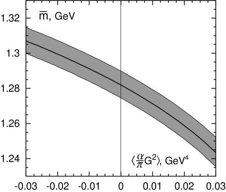
Figure 12: The dependence of $\overline{m}(\overline{m})$ on $\langle 0|\alpha_{s}/\pi)G^{2}|0\rangle$ obtained at $n=10$,  $Q^{2}=0.98\cdot 4m^{2}$ and $\alpha_{s}(Q^{2}+\overline{m}^{2})$.

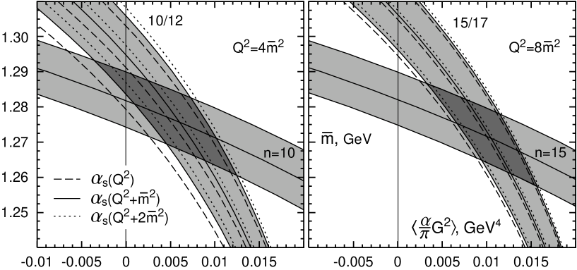
Figure 13: The dependence of $\overline{m}(\overline{m})$ on $\langle 0|(\alpha_{s}/\pi)G^{2}|0\rangle$ obtained from the moments (horizontal bands) and their ratios (vertical bands) at different $\alpha_{s}$. The left-hand figure: $Q^{2}=4\overline{m}^{2}$,   $n=10$,   $M_{10}/M_{12}$; the right-hand figure – $Q^{2}=8\overline{m}^{2}$,   $n=15$,   $M_{15}/M_{17}$.

It is also necessary to choose the scale - normalization point $\mu^{2}$ where $\alpha_{s}(\mu^{2})$ is taken. In (110)  $R(s)$ is a physical value and cannot depend on $\mu^{2}$. Since, however, we take into account in (110) only three terms, at unsuitable choice of $\mu^{2}$ such $\mu^{2}$ dependence may arise due to neglected terms. At large $Q^{2}$ the natural choice is $\mu^{2}=Q^{2}$. It can be thought that at $Q^{2}=0$ the reasonable scale is $\mu^{2}=\overline{m}^{2}$, though some numerical factor is not excluded in this equality. That is why it is reasonable to take interpolation form

$$\mu^{2}=Q^{2}+\overline{m}^{2},$$ (113)

but to check the dependence of final results on a possible factor at $\overline{m}^{2}$. Equalling theoretical value of some moment at fixed $Q^{2}$ (in the region where $M^{(1)}_{n}$ and $M^{(2)}_{n}$ are small) to its experimental value one can find the dependence of $\overline{m}$ on $\langle(\alpha_{s}/\pi)G^{2}\rangle$ (neglecting the terms $\sim\langle G^{3}\rangle$). Such a dependence for $n=10$ and $Q^{2}/4m^{2}=0.98$ is presented in Fig.12.

To fix both $\overline{m}$ and $\langle(\alpha_{s}/\pi)G^{2}\rangle$ one should, except for moments, take their ratios. Fig.13 shows the value of $\overline{m}$ obtained from the moment $M_{10}$ and the ratio $M_{10}/M_{12}$ at $Q^{2}=4m^{2}$ and from the moment $M_{15}$ and the ratio $M_{15}/M_{17}$ at $Q^{2}=8m^{2}$. The best values of masses of charmed quark and gluonic condensate are obtained from fig.13:

$${\bar{m}}({\bar{m}}^{2})\,=\,1.275\pm 0.015\,{\rm GeV}\;,\qquad\left<{\alpha_{s}\over\pi}G^{2}\right>\,=\,0.009\pm 0.007\,{\rm GeV}^{4}$$ (114)

The calculation shows, that the influence of continuum – the last term in eq.(107) is completely negligible. Up to now the corrections $\sim\langle G^{3}\rangle$ were not taken into account. It appears that in the region of $n$ and $Q^{2}$ used to find $\overline{m}$ and gluonic condensate they are comparatively small and, practically, not changing $\overline{m}$, increase $\langle(\alpha_{s}/\pi)G^{2}\rangle$ by $10-20\%$ if the term $\sim\langle G^{3}\rangle$ is estimated according to (29) at $\rho_{c}=0.5fm$.

It should be noted that improvement of the accuracy of $\Gamma_{J/\psi\to ee}$ would make it possible to precise the value of gluonic condensate: the widths of horizontal bands in fig.13 are determined mainly just by this error. In particular, this, perhaps, would allow one to exclude the zero value of gluonic condensate, that would be extremely important. Unfortunately, eq.(114) does not allow one to do it for sure. Diminution of theoretical errors which determine the width of vertical bands seems to be less real.

In order to check the results (114) for gluon condensate the pseudoscalar and axial-vector channels in charmonia were considered. The same method of moments was used and the regions in the space $(n,Q^{2})$ were found, where higher order perturbative and OPE terms are small. In the pseudoscalar case it was obtained [118] that, if for $\overline{m}$ the value (114) is accepted and the contribution of $\langle 0|G^{4}|0\rangle$ condensate may be neglected, then there follows the upper limit for gluon condensate

$$\langle 0|\frac{\alpha_{s}}{\pi}~{}G^{2}|0\rangle<0.008~{}GeV^{4}$$ (115)

The contribution of $D=6$ condensate $\langle 0|G^{3}|0\rangle$ is shown to be small. If $\langle G^{4}\rangle$ condensate is accounted and its value is estimated by factorization hypothesis, then the upper limit for gluon condensate increases to

$$\langle 0|\frac{\alpha_{s}}{\pi}~{}G^{2}|0\rangle<0.015~{}GeV^{4}$$ (116)

In [119] the case of the axial-vector channel in charmonia was investigated and very strong limitations on gluon condensate were found:

$$\langle 0|\frac{\alpha_{s}}{\pi}~{}G^{2}|0\rangle=0.005^{+0.001}_{-0.004}~{}GeV^{4}$$ (117)

Unfortunately, (117) does not allow one to exclude the zero value for gluon condensate. It should be mentioned, that the allowed region in $(n,Q^{2})$ space, where all corrections are small, is very narrow in this case, what does allow us in [119] to check the result (117) by studying some other regions in $(n,Q^{2})$, as it was done in the two previous cases – vector and pseudoscalar.

Let us now turn the problem around and try to predict the width $\Gamma_{J/\psi\to ee}$ theoretically. In order to avoid the wrong circle argumentation we do not use the condensate value just obtained, but take the limitation $\left<{\alpha_{s}\over\pi}G^{2}\right>=0.006\pm 0.012\,{\rm GeV}^{4}$ found from $\tau$-decay data. Then, the mass limits ${\bar{m}}=1.28-1.33\,{\rm GeV}$ can be found from the moment ratios exhibited above, which do not depend on $\Gamma_{J/\psi\to ee}$ if the contributions of higher resonances is approximated by continuum (the accuracy of such approximation is about $3\%$). The substitution of these values of ${\bar{m}}$ into the moments gives

$$\Gamma^{\rm theor}_{J/\psi\to ee}\,=\,4.9\pm 0.8\,{\rm keV}$$ (118)

in comparison with experimental value $\Gamma_{J/\psi\to ee}=5.26\pm 0.37\,{\rm keV}$. Such a good coincidence of the theoretical prediction with experimental data is a very impressive demonstration of the QCD sum rules effectiveness. It must be stressed, that while obtaining (118) no additional input were used besides the condensate restriction taken from Eq.(92) and the value of $\alpha_{s}(m_{\tau}^{2})$.

7.2 The attempts to sum up the Coulomb-like corrections. Recent publications

Sometimes when considering the heavy quarkonia sum rules the Coulomb-like corrections are summed up [120]-[124]. The basic argumentation for such summation is that at $Q^{2}=0$ and high $n$ only small quark velocities $v\mathrel{\mathchoice{\lower 3.6pt\vbox{\halign{$\mathsurround=0pt\displaystyle\hfil#\hfil$\cr<\crcr\sim\crcr}}}{\lower 3.6pt\vbox{\halign{$\mathsurround=0pt\textstyle\hfil#\hfil$\cr<\crcr\sim\crcr}}}{\lower 3.6pt\vbox{\halign{$\mathsurround=0pt\scriptstyle\hfil#\hfil$\cr<\crcr\sim\crcr}}}{\lower 3.6pt\vbox{\halign{$\mathsurround=0pt\scriptscriptstyle\hfil#\hfil$\cr<\crcr\sim\crcr}}}}1/\sqrt{n}$ are essential and the problem becomes nonrelativistic. So it is possible to perform the summation with the help of well known formulae of nonrelativistic quantum mechanics for $|\psi(0)|^{2}$ in case of Coulomb interaction (see [125]).

This method was not used here for the following reasons:

1. The basic idea of our approach is to calculate the moments of the polarization operator in QCD by applying the perturbation theory and OPE (l.h.s. of the sum rules) and to compare it with the r.h.s. of the sum rules, represented by the contribution of charmonium states (mainly by $J/\psi$ in vector channel). Therefore it is assumed, that the theoretical side of the sum rule is dual to experimental one, i.e. the same domains of coordinate and momentum spaces are of importance at both sides. But the charmonium states (particularly, $J/\psi$) are by no means the Coulomb systems. A particular argument in favor of this statement is the ratio $\Gamma_{J/\psi\to ee}/\Gamma_{\psi^{\prime}\to ee}=2.4$. If charmonia were nonrelativistic Coulomb system, $\Gamma_{\psi\to ee}$ would be proportional to $|\psi(0)|^{2}\sim 1/(n_{r}+1)^{3}$, and since $\psi^{\prime}$ is the first radial excitation with $n_{r}=1$, this ratio would be equal to 8 (see also [125]).

2. The heavy quark-antiquark Coulomb interaction at large distances $r>r_{\rm conf}\sim 1\,{\rm GeV}^{-1}$ is screened by gluon and light quark-antiquark clouds, resulting in string formation. Therefore the summation of Coulombic series makes sense only when the Coulomb radius $r_{\rm Coul}$ is below $r_{\rm conf}$. (It must be taken in mind, that higher order terms in Coulombic series represent the contributions of large distances, $r\gg r_{\rm Coul}$.) For charmonia we have

$$r_{\rm Coul}\,\approx\,{2\over m_{c}C_{F}\alpha_{s}}\,\approx\,4\,{\rm GeV}^{-1}$$ (119)

It is clear, that the necessary condition $R_{\rm Coul}<R_{\rm conf}$ is badly violated for charmonia. This means that the summation of the Coulomb series in case of charmonium would be a wrong step.

3. The analysis is performed at $Q^{2}/4{\bar{m}}^{2}\geq 1$. At large $Q^{2}$ the Coulomb corrections are suppressed in comparison with $Q^{2}=0$. It is easy to estimate the characteristic values of the quark velocities. At large $n$ they are $v\approx\sqrt{(1+Q^{2}/4m^{2})/n}$. In the region $(n,Q^{2})$ the exploited above quark velocity $v\sim 1/\sqrt{5}\approx 0.45$ is not small and not in the nonrelativistic domain, where the Coulomb corrections are large and legitimate.

Nevertheless let us look on the expression of $R_{c}$, obtained after summation of the Coulomb corrections in the nonrelativistic theory [126]. It reads (to go from QED to QCD one has to replace $\alpha\to C_{F}\alpha_{s}$, $C_{F}=4/3$):

$$R_{c,\,{\rm Coul}}\,=\,{3\over 2}\,{\pi C_{F}\alpha_{s}\over 1-e^{-x}}\,=\,{3\over 2}\,v\left(\,1\,+\,{x\over 2}\,+\,{x^{2}\over 12}\,-\,{x^{4}\over 720}\,+\,\ldots\,\right)$$ (120)

where $x=\pi C_{F}\alpha_{s}/v$. At $v=0.45$ and $\alpha_{s}\approx 0.26$ the first 3 terms in the expansion (120), accounted in our calculations, reproduce the exact value of $R_{c,\,{\rm Coul}}$ with the accuracy $1.6\%$. Such deviation leads to the error of the mass ${\bar{m}}$ of order $(1-2)\times 10^{-3}\,{\rm GeV}$, which is completely negligible. In order to avoid misunderstanding, it must be mentioned, that the value of $R_{c\,{\rm Coul}}$, computed by summing the Coulomb corrections in nonrelativistic theory has not too much in common with the real physical situation. Numerically, at chosen values of the parameters, $R_{c\,{\rm Coul}}\approx 1.8$, while the real value (both experimental and in the perturbative QCD) is about $1.1$. The goal of the arguments, presented above, was to demonstrate, that even in the case of Coulombic system our approach would have a good accuracy of calculation.

At $v=0.45$ the momentum transfer from quark to antiquark is $\Delta p\sim 1\,{\rm GeV}$. (This is a typical domain for QCD sum rule validity.) In coordinate space it corresponds to $\Delta r_{q{\bar{q}}}\sim 1\,{\rm GeV}^{-1}$. Comparison with potential models [126] demonstrates, that in this region the effective potential strongly differs from Coulombic one.

4. Large compensation of various terms in the expression for the moments in $\overline{\rm MS}$ scheme is not achieved, if only the Coulomb terms are taken into account. This means, that the terms of non-Coulombic origin are more important here, than Coulombic ones.

For all these reasons the summation of nonrelativistic Coulomb corrections is inadequate in the problem in view: it will not improve the accuracy of calculations, but would be misleading.

In the recent publication [127] it is claimed, that gluon condensate is much larger than the presented above values, it was found $\langle 0|(\alpha_{s}/\pi)~{}G^{2}|0\rangle=0.062\pm 0.019~{}GeV^{4}$. The author of [127] considered the model, where hadronic spectrum is represented by infinite number of vector mesons. The polarization operator, calculated in this model was equalled to those in QCD, given by perturbative and OPE terms. The value of gluon condensate was found from this equality. The zero width approximation was used for vector mesons. It is clear, however, that the account of non-zero widths results in the terms of the same type, proportional to $1/Q^{4}$, as the contribution of gluon condensate. The sign of these terms is such, that they lead to diminishing of gluon condensate. Namely, after accounting for $\rho$-meson width, the value of gluon condensate decreases by a factor of 2. For this reason the results of [127] are not reliable.

8 Valence quark distributions in nucleon at low $Q^{2}$ and the condensates

Quark and gluon distributions in hadrons are not fully understood in QCD. QCD predicts the evolution of these distributions with $Q^{2}$ in accord with the Dokshitzer-Gribov-Lipatov-Altarelli-Parisi (DGLAP) [128]-[130] equations, but not the initial values from which this evolution starts. The standard way of determination of quark and gluon distributions in nucleon is the following [131]-[135] (for the recent review see [136]). At some $Q^{2}=Q^{2}_{0}$ (usually, at low or intermediate $Q^{2}\sim 2-5GeV^{2}$) the form of quark (valence and sea) and gluon distributions is assumed and characterized by the number of free parameters. Then, by using DGLAP equations, quark and gluon distributions are calculated at all $Q^{2}$ and $x$ and compared with the whole set of the data on deep inelastic lepton-nucleon scattering (sometimes also with prompt photon production, jets at high $p_{\bot}$ etc). The best fit for the parameters is found and, therefore, quark and gluon distributions are determined at all $Q^{2}$, including their initial values $q(Q^{2}_{0},x)$,  $g(Q^{2}_{0},x)$. Evidently, such an approach is not completely satisfactory from theoretical point of view - it would be desirable to determine the initial distribution directly from QCD. In QCD calculation valence quark distributions in nucleon essentially depend on vacuum condensate, particularly, on gluon condensate. Therefore, the comparison of valence quark distributions calculated in QCD with those , found by the fit to the data, allows one to check the values of condensates obtained by consideration of quite different physical phenomena. For all these reasons it is desirable to find quark and gluon distribution in nucleon at low $Q^{2}\sim 2-5GeV^{2}$ basing directly on QCD.

The method of calculation of valence quark distributions at low $Q^{2}(Q^{2}=2-5~{}GeV^{2})$ was suggested in [137] and developed in [138]-[140]. Recently, the method had been improved and valence quark distributions in pion [141] and transversally and longitudinally polarized $\rho$-meson [142] had been calculated, what was impossible in the initial version of the method. The idea of the approach (in the improved version) is to consider the imaginary part (in $s$-channel) of a four-point correlator $\Pi(p_{1},p_{2},q,q^{\prime})$ corresponding to the non-forward scattering of two quark currents, one of which has the quantum numbers of hadron of interest (in our case – of proton) and the other is electromagnetic (or weak). It is supposed that virtualities of the photon $q^{2},q^{\prime 2}$ and hadron currents $p^{2}_{1},p^{2}_{2}$ are large and negative $|q^{2}|=|q^{\prime 2}|\gg|p^{2}_{1}|,~{}|p^{2}_{2}|\gg R^{-2}_{c}$, where $R_{c}$ is the confinement radius. It was shown in [137] that in this case the imaginary part in $s$-channel $[s=(p_{1}+q)^{2}]$ of $\Pi(p_{1},p_{2};q,q^{\prime})$ is dominated by a small distance contribution at intermediate $x$. (The standard notation is used: $x$ is the Bjorken scaling variable, $x=-q^{2}/2\nu$ , $\nu=p_{1}q)$. The proof of this statement is given in ref.[138]. So, in the mentioned above domain of $q^{2},q^{\prime 2}$,  $p^{2}_{1},p^{2}_{2}$ and intermediate $x$  $Im\Pi(p,p_{2};q,q^{\prime})$ can be calculated using the perturbation theory and the operator product expansion in both sets of variables $q^{2}=q^{\prime 2}$ and $p^{2}_{1},p^{2}_{2}$. Only the lowest twist terms, corresponding to condition $\mid p^{2}_{1}/q^{2}\mid\ll 1$, $\mid p^{2}_{2}/q^{2}\mid\ll 1$ are considered.

The approach is inapplicable at small $x$ and $x$ close to 1. This can be easily understood for physical reasons. In deep inelastic scattering at large $|q^{2}|$ the main interaction region in space-time is the light-cone domain and longitudinal distances along the light-cone are proportional to $1/x$ and become large at small $x$ [143, 144]. For OPE validity it is necessary for these longitudinal distances along light-cone to be also small, that is not the case at small $x$. At $1-x\ll 1$ another condition of applicability of the method is violated. The total energy square $s=Q^{2}(1/x-1)+p^{2}_{1}$  $Q^{2}=-q^{2}$ is not large at $1-x\ll 1$. Numerically, the typical values to be used below are $Q^{2}\sim 5~{}GeV^{2}$,   $p^{2}_{1}\sim-1~{}GeV^{2}$. Then, even at $x\approx 0.7$,   $s\approx 1~{}GeV^{2}$, i.e., at such $x$ we are in the resonance, but not in the scaling region. So, one may expect beforehand, that our method could work only up to $x\approx 0.7$. The inapplicability of the method at small and large $x$ manifests itself in the blow-up of higher order terms of OPE. More precise limits on the applicability domain in $x$ will be found from the magnitude of these terms.

The further procedure is common for QCD sum rules. On one hand the four-point correlator $\Pi(p_{1},p_{2};q,q^{\prime})$ is calculated by perturbation theory and OPE.On the other hand, the double dispersion representation in $p^{2}_{1},p^{2}_{2}$ in terms of physical states contributions is written for the same correlator and the contribution of the lowest state is extracted using the Borel transformation. By equalling these two expression the desired quark distribution is found. Valence quark distributions in proton according to this method were calculated in [145]. The basic results of [145] are presented below.

Consider the 4-current correlator which corresponds to the virtual photon scattering on the quark current with quantum number of proton:

$$T^{\mu\nu}(p_{1},p_{2},q,q^{\prime})=-i\int d^{4}xd^{4}yd^{4}z\cdot e^{i(p_{1}x+qy-p_{2}z)}\cdot$$

$$\cdot\langle 0|T\{\eta(x),~{}j^{u,d}_{\mu}(y),j^{u,d}_{\nu}(0),~{}\bar{\eta}(z)\}|0\rangle,$$ (121)

where $\eta(x)$ is the three-quark current (94). Choose the currents in the form $j^{u}_{\mu}=\bar{u}\gamma_{\mu}u$,  $j^{d}_{\mu}=\bar{d}\gamma_{\mu}d$, i.e. as an electromagnetic current which interacts only with $u(d)$ quark (with unit charges). Such a choice allows us to get sum rules separately for distribution functions of $u$ and $d$ quarks. Let us take the hadronic currents momenta to be nonequal, perform the independent Borel transformation over $p^{2}_{1}$ and $p^{2}_{2}$ and only at very end put the Borel parameters $M^{2}_{1}$ and $M^{2}_{2}$ to be equal. The described procedure allows one to kill nondiagonal transitions matrix elements of the type

$$\langle 0|j^{h}|h^{*}\rangle\langle h^{*}|j^{el}_{\mu}(y)j^{el}_{\nu}(0)|h\rangle\langle h|j^{h}|0\rangle$$ (122)

and thus makes it possible to separate the diagonal transition of interest

$$\langle 0|j^{h}|h\rangle\langle h|j^{el}_{\mu}(y)j^{el}_{\nu}(0)|h\rangle\langle h|j^{h}|0\rangle.$$ (123)

As was shown in Ref.[145] the sum rules for nucleon have the form

$$\frac{2\pi}{4M^{4}}~{}\frac{\bar{\lambda}^{2}_{p}}{32\pi^{4}}~{}xq^{u,d}(x)e^{-m^{2}/M^{2}}=ImT^{0}_{u,d}+\mbox{Power~{} corrections}$$ (124)

Here the l.h.s is the phenomenological side of the sum rule – the proton state contribution, $\bar{\lambda}_{p}$ is defined in (100). In numerical calculations it will be put equal $\bar{\lambda}^{2}_{p}=3.0~{}GeV^{6}$. The right hand side is calculated in QCD. The excited states contribution – the continuum is identifyed with the contribution of bare loop diagram, starting from continuum threshold value $s_{0}$ and is transferred to the l.h.s. of the sum rule. The bare loop contribution to the sum rules is represented in Fig.14.

Figure 14: Bare loop diagrams, corresponding to unit operator contribution for $u$- and $d$-quarks (respectively, a) and b)).

The results after the double Borel transformation are

$$ImT^{0}_{u(d)}=\varphi^{u(d)}_{0}(x)\frac{M^{2}}{32\pi^{3}}~{}E_{2}(s_{0}/M^{2})$$ (125)

where

$$\varphi^{u}_{0}(x)=x(1-x)^{2}(1+8x),~{}~{}\varphi^{d}_{0}(x)=x(1-x)^{2}(1+2x),$$ (126)

$E_{2}(z)$ is given by (98) The substitution of eq.(125) into the sum rules (124) results in

$$xq(x)_{0}^{u(d)}=\frac{2M^{6}e^{m^{2}/M^{2}}}{\bar{\lambda}^{2}_{p}}~{}\varphi_{0}^{u(d)}(x)\cdot E_{2}\Biggl{(}\frac{s_{0}}{M^{2}}\Biggr{)}$$ (127)

Making use of relation $\bar{\lambda}^{2}_{p}e^{-m^{2}/M^{2}}=M^{6}E_{2}$ which follows from the sum rule for the nucleon mass (see (95)) in the same approximation), we get

$$\int\limits^{1}_{0}~{}d_{0}(x)dx=1,~{}~{}~{}\int\limits^{1}_{0}~{}u_{0}(x)dx=2$$ (128)

In the bare loop approximation there also appears the sum rule for the second moment:

$$\int\limits^{1}_{0}~{}x(q^{u}_{0}(x)+q^{d}_{0}(x))dx=1$$ (129)

Analogously to [138] one can show that relations (128),(129) hold also when taking into account power corrections proportional to the quark condensate square in the sum rules for the 4-point correlator and in the sum rules for the nucleon mass. Relations (128) reflect the fact that proton has two $u$-quarks and one $d$-quark. Relation (129) expresses the momentum conservation law – in the bare loop approximation all momentum is carried by valence quarks. Therefore, the sum rules (128),(129) demonstrate that the zero order approximation is reasonable.

Let us calculate the perturbative corrections to bare loop and restrict ourselves by the leading order (LO) corrections proportional to $lnQ^{2}_{0}/\mu^{2}$, where $Q^{2}_{0}$ is the point, where the quark distributions $q(x,Q^{2}_{0})$ is calculated and $\mu^{2}$ is the normalization point. In our case it is reasonable to choose $\mu^{2}$ to be equal to the Borel parameter $\mu^{2}=M^{2}$. The results take the form:

$$d^{LO}(x)=d_{0}(x)\left\{1+\frac{4}{3}ln(Q^{2}_{0}/M^{2})\cdot\frac{\alpha_{s}(Q^{2}_{0})}{2\pi}\cdot\right.$$

$$\left.\Biggl{[}1/2+x+ln((1-x)^{2}/x)+\frac{-5-17x+16x^{2}+12x^{3}}{6(1-x)(1+2x)}-\frac{(3-2x)x^{2}ln(1/x)}{(1-x)^{2}(1+2x)}\Biggr{]}\right\}$$ (130)

$$u^{LO}(x)=u_{0}(x)\cdot\left\{1+\frac{4}{3}~{}\frac{\alpha_{s}(Q^{2}_{0})}{2\pi}ln(Q^{2}_{0}/M^{2})\Biggl{[}1/2+x+ln(1-x)^{2}/x+\right.$$

$$\left.\frac{7-59x+46x^{2}+48x^{3}}{6(1-x)(1+8x)}-\frac{(15-8x)x^{2}ln(1/x)}{(1-x)^{2}(1+8x)}\Biggr{]}\right\}$$ (131)

where $u_{0}(x)$ and $d_{0}(x)$ are bare loop contributions, given by (127).

The contributions of gluon condensate to $u$ and $d$-quarks distribution were found to be (the ratios to bare loop contributions are presented):

$$\frac{u(x)_{\langle G^{2}\rangle}}{u_{0}(x)}=\frac{\langle(\alpha_{s}/\pi)G^{2}\rangle}{M^{4}}\cdot\frac{\pi^{2}}{12}~{}\frac{(11+4x-31x^{2})}{x(1-x)^{2}(1+8x)}~{}E_{0}(s_{0}/M^{2})/E_{2}(\frac{s_{0}}{M^{2}})$$ (132)

$$\frac{d(x)_{\langle G^{2}\rangle}}{d_{0}(x)}=-\frac{\langle(\alpha_{s}/\pi)G^{2}\rangle}{M^{4}}\frac{\pi^{2}}{6}~{}\frac{(1-2x^{2})}{x^{2}(1-x)^{2}(1+2x)}E_{0}(s_{0}/M^{2})/E_{2}(\frac{s_{0}}{M^{2}})$$ (133)

The contributions of quark condensate – the terms, proportional to $\alpha_{s}(M^{2})\langle 0\mid\bar{q}q\mid 0\rangle^{2}$ are few times smaller, than the contributions of gluon condensate and are not presented here. (They can be found in Ref.[145]).

Figure 15: $d$- and $u$-quark distribution at various values of gluon condensate ($\langle(\alpha_{s}/\pi)G^{2}\rangle=0.012,0.06$ and 0 GeV⁴, respectively dotted, solid and dashed lines). Thick solid line corresponds to the results of [131].

The final result for valence quark distribution in proton are of the form

$$xu(x)=\frac{M^{6}e^{m^{2}/M^{2}}}{\bar{\lambda}^{2}_{N}}2x(1-x)^{2}(1+8x)E_{2}(\frac{s_{0}}{M^{2}})\left\{\Biggl{[}1+\frac{u^{LO}(x,Q^{2}_{0})}{u_{0}(x)}\Biggr{]}+\right.$$

$$\left.+\frac{1}{u_{0}(x)}[u(x)_{\langle G^{2}\rangle}+u(x)_{\alpha_{s}\langle\bar{q}q\rangle^{2}}]\right\}$$ (134)

$$xd(x)=\frac{M^{6}e^{m^{2}/M^{2}}}{\bar{\lambda}^{2}_{N}}2x(1-x)^{2}(1+2x)E_{2}(\frac{s_{0}}{M^{2}})\left\{\Biggl{[}1+\frac{d^{LO}(x,Q^{2}_{0})}{d_{0}(x)}\Biggr{]}+\right.$$

$$\left.+\frac{1}{d_{0}(x)}[d(x)_{\langle G^{2}\rangle}+d(x)_{\alpha_{s}\langle\bar{q}q\rangle^{2}}]\right\}$$ (135)

The valence $u$ and $d$ quark distribution calculated according to (134),(135) for various $\langle(\alpha_{s}/\pi)G^{2}\rangle=0.00,0.006,0.012~{}GeV^{4}$ are shown in Fig.15.

The following values of parameters were used: $\alpha_{s}\langle 0\mid\bar{q}q\mid 0\rangle^{2}$ given by (85), $\bar{\lambda}^{2}_{p}=3.0~{}GeV^{6}$, $\lambda_{QCD}=250~{}GeV$, $s_{0}=2.5~{}GeV^{2}$, $Q^{2}_{0}=5~{}GeV^{2}$. The contribution of $\langle G^{3}\rangle$ condensate was estimated on the basis of instanton model – Eq.(29). This contribution may influence $u$ and $d$-quark distributions at $x\mathrel{\mathchoice{\lower 3.6pt\vbox{\halign{$\mathsurround=0pt\displaystyle\hfil#\hfil$\cr<\crcr\sim\crcr}}}{\lower 3.6pt\vbox{\halign{$\mathsurround=0pt\textstyle\hfil#\hfil$\cr<\crcr\sim\crcr}}}{\lower 3.6pt\vbox{\halign{$\mathsurround=0pt\scriptstyle\hfil#\hfil$\cr<\crcr\sim\crcr}}}{\lower 3.6pt\vbox{\halign{$\mathsurround=0pt\scriptscriptstyle\hfil#\hfil$\cr<\crcr\sim\crcr}}}}0.2$ and increase both of them by 10-20%. The limits of applicability of QCD calculations are: for $u$- quark – $0.2<x<0.65$, for $d$-quark – $0.3<x<0.65$. The lower limit arises from gluon condensate contribution – it was required, that this contribution does not exceed 30%, the upper limit was determined by increasing of perturbative corrections and $\alpha_{s}\langle\bar{q}q\rangle^{2}$ terms. For comparison, Fig.15 presents the results of the fit to data basing on the solution of DGLAP equation. The LO order fit [131] is chosen, but not the more precise NLO fits [132]-[136], because QCD calculations of quark distributions were performed in LO. As is seen from Fig.15 the calculated in QCD initial (at $Q^{2}_{0}=5~{}GeV^{2}$) valence quark distributions at $0.3<x<0.7$ are in a satisfactory agreement with those found from the data. The preferred value of gluonic condensate is $\langle 0\mid(\alpha_{s}/\pi)G^{2}\mid 0\rangle=0.006~{}GeV^{4}$, the values higher than $0.012~{}GeV^{2}$ and lower than $0$, probably, may be excluded. These statements are in full accord with those obtained in the previous Chapters.

9 Conclusion

The basic parameters of QCD – $\alpha_{s}(Q^{2})$ and the values of vacuum condensates, determining hadron physics at low momentum transfers $(Q^{2}\sim 1-5~{}GeV^{2})$, are reliably determined by the theory. It was demonstrated, that the values of these parameters, found by consideration of various processes are in a good agreement with one another. The values of $u,d,s$ quark masses and their ratios are known now with a good precision – about 10-15% in the ratios and about 20% in the mass absolute values. The precision in charmed quark mass value $\overline{m}_{c}(\overline{m}_{c})$ in $\overline{MS}$ renormalization scheme is extremingly high – about 1%. The knowledge of $\alpha_{s}(Q^{2})$ and condensates makes it possible to find the polarization operators of vector and axial currents at $Q^{2}\geq 1~{}GeV^{2}$ with high precision. In such calculation high order perturbative terms – $\sim\alpha^{2}_{s}$ and, in some cases, $\sim\alpha^{3}_{s}$ must be accounted. Therefore, we have now a good basis for theoretical description of many physical phenomena in low energy QCD – hadron masses, their static properties, quark distributions in hadrons etc. Of course, at even lower momentum transfer, $Q^{2}\mathrel{\mathchoice{\lower 3.6pt\vbox{\halign{$\mathsurround=0pt\displaystyle\hfil#\hfil$\cr<\crcr\sim\crcr}}}{\lower 3.6pt\vbox{\halign{$\mathsurround=0pt\textstyle\hfil#\hfil$\cr<\crcr\sim\crcr}}}{\lower 3.6pt\vbox{\halign{$\mathsurround=0pt\scriptstyle\hfil#\hfil$\cr<\crcr\sim\crcr}}}{\lower 3.6pt\vbox{\halign{$\mathsurround=0pt\scriptscriptstyle\hfil#\hfil$\cr<\crcr\sim\crcr}}}}1~{}GeV^{2}$, the approach, exploited in this review and based on perturbation theory and OPE, does not work: the confinement mechanism and the mechanism of spontaneous symmetry breaking are acting in full strength. The construction of various models is inavoidable here. But for such models the knowledge of basic QCD parameters is also quite important – they may play the role of cornerstones for the models.

I summarize here the final values of $\alpha_{s}$ and condensates:

$$\alpha_{s}(m^{2}_{\tau})=0.340\pm 0.015~{}~{}~{}\overline{MS}-\mbox{scheme}$$ (136)

$$\langle 0\mid\frac{\alpha_{s}}{\pi}G^{2}_{\mu\nu}\mid 0\rangle=0.005\pm 0.004~{}GeV^{2}$$ (137)

$$\langle 0\mid\bar{q}q\mid 0\rangle_{1~{}GeV}=-(1.65\pm 0.15)\cdot 10^{-2}~{}GeV^{3},~{}~{}q=u,d$$ (138)

$$\alpha_{s}\langle 0\mid\bar{q}q\mid 0\rangle^{2}=(1.5\pm 0.2)\cdot 10^{-4}~{}GeV^{6}$$ (139)

(In determination of (139) the factorization hypothesis is assumed.) The values of errors, given in ((137)-(139) are a bit uncertain, since the procedure of averaging of errors in different processes is subjective in essential way.

10 Acknowledgements

I am thankful to my coauthors K.N.Zyablyuk, A.G.Oganesian, A.V.Samsonov and B.V.Geshkenbein for their cooperations in the papers, which content was included in this review and to N.S.Libova and M.N.Markina for their help in the preparation of the manuscript. This work was supported in part by U.S.Civilian Research and Development Foundation (CRDF) Cooperative Grant Program, Project RUP2-2621-MO-04, RFBR grant 03-02-16209 and the funds from EC to the project “Study of Strongly Interacting Matter” under contract 2004 No.R113-CT-2004-506078.

References

- [1] M.A. Shifman, A.I. Vainshtein and V.I. Zakharov, Nucl. Phys. B 147 (1979) 385, 448
- [2] J. Gasser and H. Leutwyler, Nucl. Phys. B 94 (1975) 269
- [3] J. Gasser and H. Leutwyler, Phys. Rep. 87 (1982) 77
- [4] S. Weinberg, in: A Festschrift for I.I. Rabi ed. by L. Motz, Trans. New York Acad. Sci., Ser.II, 38 (1977) p. 185
- [5] R. Dashen, Phys. Rev. 183 (1969) 1245
- [6] J. Gasser and H. Leutwyler, Nucl. Phys. B 250 (1985) 469
- [7] J. Donoghue and A. Perez, Phys. Rev. D 55 (1997) 7075
- [8] J. Bijnens and J. Prades, Nucl. Phys. B 490 (1997) 293
- [9] J. Gasser and H. Leutwyler, Nucl. Phys. B 250 (1985) 539
- [10] J. Kambor, C. Wiesendanger and D. Wyler, Nucl. Phys. B 465 (1996) 215
- [11] A.V. Anisovich and H. Leutwyler, Phys. Lett. B 375 (1996) 335
- [12] B.V. Martemyanov and V.S. Sopov, Phys. Rev. D 71 (2005) 017501
- [13] Particle Data Group, S. Eidelman et al., Phys. Lett. B 592 (2004) 1
- [14] H. Leutwyler, J. M. Phys. Soc. 6 (1996) 1, hep-ph/9602255
- [15] B.L. Ioffe and M.A. Shifman, Phys. Lett. B 95 (1980) 99
- [16] B.L. Ioffe and M.A. Shifman, Phys. Lett. B 107 (1981) 33
- [17] CLEO Collaboration, N.E. Adam et al, hep-ex/0503028
- [18] N. Nasrallah, Phys. Rev. D 70 (2004) 116001
- [19] C. Aubin et al. (MILC Collab.), hep-lat/0407028
- [20] J.A.M. Vermaseren, A.A. Larin and T. van Ritbergen, Phys. Lett. B 405 (1997) 327
- [21] S. Narison, QCD as a Theory of Hadrons: from Partons to Confinement, Cambridge Univ. Press, 2002, hep-ph/0202200
- [22] M. Jamin and A. Pich, hep-ph/0411278
- [23] P.A. Baikov, K.G. Chetyrkin and J.H. Kühn, hep-ph/0412350
- [24] G. Schierholz et al., hep-ph/0409312
- [25] C. Adami, E.G. Drukarev and B.L. Ioffe, Phys. Rev. D 48 (1993) 1441
- [26] V.L. Eletsky and B.L. Ioffe, Phys. Rev. D 48 (1993) 2304
- [27] J. Prades, Nucl. Phys. B (Proc. Suppl.) 64 (1998) 253
- [28] V.A. Novikov, M.A. Shifman, A.I. Vainstein and V.I. Zakharov, Nucl. Phys. B 249 (1985) 445
- [29] M.A. Shifman, Lecture at 1997 Yukawa International Seminar, Kyoto, 1997, Suppl.Prog.Theor.Phys., Vol. 131 (1998) p. 1
- [30] M. Gell-Mann, R.J. Oakes and B. Renner, Phys. Rev. 175 (1968) 2195
- [31] B.L. Ioffe, Physics-Uspekhi 44 (2001) 1211
- [32] B.L. Ioffe, Nucl. Phys. B 188 (1981) 317 ; Errata 192 (1982) 591
- [33] H. Leutwyler, in: At the Frontier of Particle Physics, Handbook of QCD, Boris Ioffe Festschrift, ed. by M. Shifman, World Scientific, Vol. 1 (2001) p. 271
- [34] U. Meissner, ibid, p. 417
- [35] P. Gerber and H. Leutwyler, Nucl. Phys. B 321 (1989) 387
- [36] P. Chen et al., Phys. Rev. D 64 (2001) 014503
- [37] V.M. Belyaev and B.L. Ioffe, Sov. Phys. JETP 56 (1982) 493
- [38] H.G. Dosch and S. Narison, Phys. Lett. B 417 (1998) 173
- [39] A.Di Giacomo and Yu.Simonov, hep-ph/0404044
- [40] M.A. Shifman, Pis’ma v ZhETF 24 (1976) 376
- [41] V.A. Novikov, M.A. Shifman, A.I. Vainstein and V.A. Zakharov, Phys. Lett. B 86 (1979) 34+7
- [42] S.N. Nikolaev and A.V. Radyushkin, Sov. J. Nucl. Phys. 39 (1984) 91
- [43] B.L. Ioffe and A.V. Samsonov, Phys. At. Nucl. 63 (2000) 1448
- [44] B.L. Ioffe and A.V. Smilga, Nucl. Phys. B 232 (1984) 109
- [45] V.M. Belyaev and I.I. Kogan, Yad. Fiz. 40 (1984) 1035 I.I. Balitsky, A.V. Kolesnichenko and A.V. Yung, Yad. Fiz. 41 (1985) 282
- [46] V.M. Belyaev and I.I. Kogan, Pis’ma v ZhETF 37 (1983) 611
- [47] B.L. Ioffe and A.G. Oganesian, Phys. Rev. D 57 (1998) R6590
- [48] ALEPH Collaboration, R. Barate et al., Eur. Phys. J. C 4 (1998) 409, C 11 (1999) 599, The data files are taken from http://alephwww.cern.ch/ALPUB/paper/ paper.html
- [49] OPAL Collaboration, K. Ackerstaff et al., Eur. Phys. J. C 7 (1999) 571; G. Abbiendi et al., ibid, 13 (2002) 197
- [50] CLEO Collaboration, S.J. Richichi et al., Phys. Rev. D 60 (1999) 112002
- [51] B.L. Ioffe and K.N. Zyablyuk, Nucl. Phys. A 687 (2001) 437
- [52] B.V. Geshkenbein, B.L. Ioffe and K.N. Zyablyuk, Phys. Rev. D 64 (2001) 093009
- [53] M. Davier, A. Höcker, R. Girlanda and J. Stern, Phys. Rev. D 58 (1998) 96014
- [54] M. Davier et al., hep-ex/0312064
- [55] A. Pich, Proc. of QCD 94 Workshop, Monpellier, 1994; Nucl. Phys. B (proc.Suppl) 39 (1995) 396
- [56] W.J. Marciano and A. Sirlin, Phys. Rev. Lett. 61 (1998) 1815
- [57] E. Braaten, Phys. Rev. Lett. 60 (1988) 1606 ; Phys. Rev. D 39 (1989) 1458
- [58] S. Narison and A. Pich, Phys. Lett. B 211 (1988) 183
- [59] F. Le Diberder and A. Pich, Phys. Lett. B 286 (1992) 147
- [60] K.G. Chetyrkin, A.L. Kataev and F.V. Tkachov, Phys. Lett. B 85 (1979) 277 ; M. Dine and J. Sapirshtein, Phys. Rev. Lett. 43 (1979) 668 ; W. Celmaster and R. Gonsalves, ibid, 44 (1980) 560
- [61] L.R. Surgaladze and M.A. Samuel, Phys. Rev. Lett. 66 (1991) 560 ; S.G. Goryshny, A.L. Kataev and S.A. Larin, Phys. Lett. B 259 (1991) 144
- [62] A.L. Kataev and V.V. Starshenko, Mod. Phys. Lett. A 10 (1995) 235
- [63] P.A. Baikov, K.G. Chetyrkin and J.P. Kühn, Phys. Rev. D 67 (2003) 074026
- [64] O.V. Tarasov, A.A. Vladimirov and A.Yu. Zharkov, Phys. Lett. B 93 (1980) 429 ; S.A. Larin and J.A.M. Vermaseren, ibid, 303 (1993) 334
- [65] T. van Ritbergen, J.A.M. Vermaseren and S.A. Larin, Phys. Lett. B 400 (1997) 379
- [66] M. Czakon, hep-ph/0411261
- [67] A.V. Radyushkin, JINR E2-82-159, hep-ph/9907228
- [68] A. Pivovarov, Nuovo Cimento A 105 (1992) 813
- [69] K.G. Chetyrkin, S.G. Gorishny and V.P. Spiridonov, Phys. Lett. B 160 (1985) 149
- [70] L.-E. Adam and K.G. Chetyrkin, Phys. Lett. B 329 (1994) 129
- [71] M.S. Dubovikov and A.V. Smilga, Nucl. Phys. B 185 (1981) 109
- [72] E. Braaten and C.S. Lee, Phys. Rev. D 42 (1990) 3888
- [73] M. Davier, 8 Intern. Symposium on Heavy Flavour Physics, Southampton, England, 1999, hep-ex/9912094
- [74] ALEPH Collaboration, R. Barate et al., Eur. Phys. J. C 11 (1999) 599
- [75] OPAL Collaboration, G. Abbiendi et al., Eur. Phys. J. C 19 (2001) 653
- [76] S. Bethke, hep-ex/040702
- [77] T. Shafer and E.V. Shuryak, Rev. Mod. Phys. 70 (1998) 323
- [78] E.V. Shuryak, Nucl. Phys. B 198 (1982) 83
- [79] ”Instantons in Gauge Theories”, ed. by M. Shifman, World Scientific, 1994
- [80] N. Andrei and D.J. Gross, Phys. Rev. D 18 (1978) 468
- [81] T. Shafer and E.V. Shuryak, Phys. Rev. Lett. 86 (2001) 3973
- [82] Y.L. Luke, “Mathematical functions and their approximations”, NY, Academic Press 1975; H. Bateman and A. Erdelyi, “Higher transcendental functions”, Vol. I, Krieger, Melbourne, FL, 1953
- [83] S.J. Brodsky, G.P. Lepage and P.B. Mackenzie, Phys. Rev. D 28 (1983) 228
- [84] S.J. Brodsky, V.S. Fadin, V.T. Kim, L.N. Lipatov and G.B. Pivovarov, JETP Lett. 70 (1999) 155
- [85] S.J. Brodsky, S. Menke, C. Merino and J. Rathsman, Phys. Rev. D 67 (2003) 055008
- [86] D.V. Shirkov, Eur. Phys. J. C 22 (2001) 331
- [87] K.A. Milton, I.L. Solovtsov and O.P. Solovtsova, Phys. Rev. D 64 (2001) 016005
- [88] M.S. Dubovikov and A.V. Smilga, Yad. Fiz. 37 (1983) 984 A. Grozin and Y. Pinelis, Phys. Lett. B 166 (1986) 429
- [89] K.N. Zyablyuk, hep-ph/0404230.
- [90] K.G. Chetyrkin, S.G. Gorishny and V.P. Spiridonov, Phys. Lett. B 160 (1985) 149
- [91] L.-E. Adam and K.G. Chetyrkin, Phys. Lett. B 329 (1994) 129
- [92] J. Bijnens, E. Gamiz and J. Prades, JHEP 10 (2001) 009
- [93] V. Cirigliano, E. Golowich and K.Maltman, Phys. Rev. D 68 (2003) 054013
- [94] S. Friot, D. Greynat and E. de Rafael, JHEP 10 (2004) 043
- [95] J. Rojo and J. I. Lattore, JHEP 0401 (2004) 055
- [96] C.A. Dominguez and A. Schilcher, Phys. Lett. B 581 (2004) 193
- [97] S. Chiulli, G. Sebu, K. Schilcher and G. Speiberger, Phys. Lett. B 595 (2004) 359
- [98] S. Narison, hep-ph/0412152
- [99] ALEPH Coollaboration, R. Barate, et al., Z. Phys. C 76 (1997) 15
- [100] S.I. Eidelman, L.M. Kurdadze and A.I. Vainstein, Phys. Lett. B 82 (1979) 278
- [101] A. Höcker, hep-ph/0410081
- [102] B.L. Ioffe, Z. Phys. C 18 (1983) 67
- [103] M. Jamin, Z. Phys. C 37 (1988) 635 ; M. Jamin, Dissertation thesis, Heidelberg preprint HD-THEP-88-19 (1988); A.A. Ovchinnikov, A.A. Pivovarov and L.R. Surguladze, Sov. J. Nucl. Phys. 48 (1988) 358; A.G. Oganesian, hep-ph/0308289
- [104] A.E. Dorokhov and N.I. Kochelev, Z. Phys. C 46 (1990) 281
- [105] H. Forkel and M.K. Banerjee, Phys. Rev. Lett. 71 (1993) 484
- [106] S.N. Nikolaev and A.V. Radyushkin, JETP Lett. 37 (1982) 526
- [107] L.J. Reinders, H.R. Rubinstein and S. Yazaki, Phys. Lett. B 138 (1984) 340
- [108] S. Narison, QCD Spectral Sum Rules, (World Scientific, 1989); Phys. Lett. B 387 (1996) 162 ; V.A. Novikov, M.A. Shifman, A.I. Vainstein, M.B. Voloshin and V.A. Zakharov, Nucl. Phys. B 237 (1984) 525 ; K.J. Miller and M.G. Olsson, Phys. Rev. D 25 (1982) 1247
- [109] P. Colangelo and A. Khodjamirian, At frontier of Particle Physics, Handbook of QCD, Boris Ioffe Festschrift, v.3, p.1495, World Scientific, 2001.
- [110] R.A. Bertlmann, Nucl. Phys. B 204 (1982) 387 ; V.N. Baier and Yu.F. Pinelis, Phys. Lett. B 116 (1982) 179 , Nucl. Phys. B 229 (1983) 29 ; G. Launer, S. Narison and R. Tarrach, Z. Phys. C 26 (1984) 433 ; R.A. Bertlmann, C.A. Dominguez, M. Loewe, M. Perrottet and E. de Rafael, Z. Phys. C 39 (1988) 231 ; P.A. Baikov, V.A. Ilyin and V.A. Smirnov, Phys. Atom. Nucl. 56 (1993) 1527; D.J. Broadhurst, P.A. Baikov, V.A. Ilyin, J. Fleischer, O.V. Tarasov and V.A. Smirnov, Phys. Lett. B 329 (1994) 103 ; B.V. Geshkenbein, Phys. Atom. Nucl. 59 (1996) 289
- [111] M. Jamin and A. Pich, Nucl. Phys. B 507 (1997) 334 ; M. Eidemüller and M. Jamin, Phys. Lett. B 498 (2001) 203 ; J.N. Kühn and M. Steinhauser, Nucl. Phys. B 619 (2001) 588
- [112] B.L. Ioffe and K.N. Zyablyuk, Eur. Phys. J. C 27 (2003) 229
- [113] V.B. Berestetsky and I.Ya. Pomeranchuk, JETP 29 (1955) 864
- [114] J. Schwinger, Particles, Sources, Fields, Addison-Wesley Publ., 1973, V.2
- [115] A.H. Hoang, J.H. Kühn and T. Teubner, Nucl. Phys. B 452 (1995) 173 ; K.G. Chetyrkin, J.H. Kühn and M. Steinhauser, Nucl. Phys. B 482 (1996) 231 ; K.G. Chetyrkin et al., Nucl. Phys. B 503 (1997) 339 ; K.G. Chetyrkin et al., Eur. Phys. J. C 2 (1998) 137
- [116] D.J. Broadhurst et al., Phys. Lett. B 329 (1994) 103
- [117] S.N. Nikolaev and A.V. Radyushkin, Sov. J. Nucl. Phys. 39 (1984) 91
- [118] K.N. Zyablyuk, JHEP 0301:081 (2003)
- [119] A.V Samsonov, hep-ph/0407199
- [120] V.A. Khoze and M.A. Shifman, Sov. Phys. Usp. 26 (1983) 387
- [121] M.B. Voloshin, Int. J. Mod. Phys. A 10 (1995) 2865
- [122] M. Jamin, A. Pich, Nucl. Phys. B 507 (1997) 334
- [123] K.G. Chetyrkin, A.H. Hoang, J.H. Kühn, M. Steinhauser and T. Teubner, Eur. Phys. J. C 2 (1998) 137
- [124] J.H. Kühn, A.A. Penin and A.A. Pivovarov, Nucl. Phys. B 534 (1998) 356
- [125] L. Landau and E. Lifshitz, Quantum Mechanics: Nonrelativistic Theory, Pergamon Press, 1977
- [126] E. Eichten et al., Phys. Rev. D 21 (1980) 203
- [127] B.V. Geshkenbein, Phys. Rev. D 70 (2004) 074027
- [128] V.N. Gribov and L.N. Lipatov, Sov. J. Nucl. Phys. 15 (1972) 438
- [129] Yu.L. Dokshitzer, Sov. Phys. JETP 46 (1977) 641
- [130] G. Altarelli and G. Parisi, Nucl. Phys. B 126 (1977) 298
- [131] M. Glück, E. Reya and A. Vogt, Z. Phys. C 53 (1992) 127
- [132] H. L. Lai et al. (CTEQ Collab.), Eur. Phys. J. C 12 (2000) 375
- [133] A.D. Martin, R.G. Roberts, W.J. Stirling and R.S. Thorne, Eur. Phys. J. C 4 (1998) 463
- [134] M. Glück, E. Reya and A. Vogt, Eur. Phys. J. C 5 (1998) 461
- [135] A.M. Cooper-Sarkar, R.C.E. Davenish and A. De Roeck, Int. J. Mod. Phys. A 13 (1998) 3385
- [136] Wu-Ki Tung, At the Frontier of Particle Physics, in: Handbook of QCD, Boris Ioffe Festschrift, ed. by M. Shifman, World Sci. 2001, v.2, p.887
- [137] B.L. Ioffe, Pis’ma v ZhETF 42 (1985) 266, JETP Lett. 42 (1985) 327
- [138] V.M. Belyaev and B.L. Ioffe, Nucl. Phys. B 310 (1988) 548
- [139] A.S. Gorsky, B.L. Ioffe, A.Yu. Khodjamirian and A.G. Oganesian, Z. Phys. C 44 (1989) 523 B.L. Ioffe and A.G.Oganesian, Z. Phys. C 69 (1995) 119
- [140] B.L. Ioffe and A.Yu. Khodjamirian, Phys. Rev. D 51 (1995) 3373
- [141] B.L. Ioffe and A. Oganesian, Eur. Phys. J. C 13 (2000) 485
- [142] B.L. Ioffe and A.G. Oganesian, Phys. Rev. D 63 (2001) 096006
- [143] V.N. Gribov, B.L. Ioffe and I.Ya. Pomeranchuk, Sov. J. Nucl. Phys. 2 (1966) 549
- [144] B.L. Ioffe, Phys. Lett. B 30 (1969) 123
- [145] B.L. Ioffe, A.G. Oganesian, Nucl. Phys. A 714 (2003) 145