Damping signatures in future neutrino oscillation experiments

Mattias Blennow, Tommy Ohlsson, and Walter Winter 

^,Division of Mathematical Physics, Department of Physics, School of Engineering Sciences, Royal Institute of Technology (KTH) – AlbaNova University Center,

Roslagstullsbacken 11, 106 91  Stockholm, Sweden

School of Natural Sciences, Institute for Advanced Study,

Einstein Drive, Princeton, NJ 08540, USA

Abstract

We discuss the phenomenology of damping signatures in the neutrino oscillation probabilities, where either the oscillating terms or the probabilities can be damped. This approach is a possibility for tests of non-oscillation effects in future neutrino oscillation experiments, where we mainly focus on reactor and long-baseline experiments. We extensively motivate different damping signatures due to small corrections by neutrino decoherence, neutrino decay, oscillations into sterile neutrinos, or other mechanisms, and classify these signatures according to their energy (spectral) dependencies. We demonstrate, at the example of short baseline reactor experiments, that damping can severely alter the interpretation of results, e.g., it could fake a value of $\sin^{2}(2\theta_{13})$ smaller than the one provided by Nature. In addition, we demonstrate how a neutrino factory could constrain different damping models with emphasis on how these different models could be distinguished, i.e., how easily the actual non-oscillation effects could be identified. We find that the damping models cluster in different categories, which can be much better distinguished from each other than models within the same cluster.

1 Introduction

Neutrino oscillations are by far the most plausible description of transitions among different neutrino flavor eigenstates [1, 2, 3, 4, 5, 6, 7]. However, there have historically been other attempts in the literature to describe these transitions with other mechanisms as well as neutrino oscillations combined with such other mechanisms. These scenarios include neutrino wave packet decoherence [8, 9, 10, 11, 12], neutrino decay [13, 14, 15, 16, 17, 18, 19, 20], oscillations into sterile neutrinos [21, 22], neutrino absorption (see, e.g., Ref. [23]), and neutrino quantum decoherence [24, 25, 26, 27, 28, 29, 30, 31, 32]. A combined scenario is, for example, the combination of neutrino oscillations and neutrino decay (see, e.g., Refs. [19, 20]). Although these other mechanisms, leading to “non-standard effects”, are not such successful descriptions for flavor transitions as neutrino oscillations are (in fact, they are strongly disfavored [7, 6]), they could still give rise to small corrections to the neutrino oscillations. These non-standard effects need to be described in a framework together with neutrino oscillations and can be constrained by current and future experiments (see, e.g., Ref. [33] for a recent review). Thus, we will assume that the leading order effect in neutrino flavor transitions is due to neutrino oscillations, whereas the next-to-leading order effects are described by different “damping mechanisms” of the neutrino oscillations.

Since any non-standard effect may point towards new interesting physics beyond the standard model, the test of small corrections due to these effects should be one of the main objectives in future high-precision neutrino oscillation physics. The assumption of standard three-flavor neutrino oscillations will inevitably lead to an erroneous derivation of the elements of the mixing matrix $U$ or the mass squared differences. We therefore define “non-oscillation effects” as any modification of the three-flavor neutrino oscillation probabilities in vacuum as well as in matter. For example, the LSND anomaly [34] could be an indication of non-oscillation effects according to this definition. Since future reactor and long-baseline neutrino oscillation experiments are expected to have high-precisions to the subleading neutrino oscillation parameters $\sin^{2}(2\theta_{13})$ and $\delta_{\mathrm{CP}}$, we mainly discuss the impact of non-oscillation effects or possible constraints on the non-oscillation effects in the context of these experiments.

In principle, one could think of many different approaches to test non-oscillation effects with future long-baseline experiments:

Neutral-currents

can be used to test the conservation of probability, i.e., $P_{\alpha e}+P_{\alpha\mu}+P_{\alpha\tau}=1$ (see, e.g., Ref. [35]). However, at long-baseline experiments, uncertainties in the neutral-current cross-sections and the charged-current contamination lead to a precision of only about $10~{}\%-15~{}\%$ [35]. In addition, even if some non-oscillation effects are found, there will be no information on the nature of the effects, whereas effects conserving the overall probability cannot be detected at all.

The detection of $\boldsymbol{\nu_{\tau}}$

can complement the information on $P_{\alpha e}$ and $P_{\alpha\mu}$ to test the conservation of probability (see, e.g., Ref. [36]). Since $\nu_{\tau}$ detection is much more sophisticated and less efficient than the detection of $\nu_{e}$ and $\nu_{\mu}$ due to the higher $\tau$ production threshold, this is also a non-trivial test. If there are non-oscillation effects, then the information will be better than in the preceding case, since one will know which neutrino oscillation probabilities are affected.

Unitarity triangles

for the lepton sector can be constructed [37, 38]. However, since there is no simple relationship between the quantities of the unitarity triangles and the neutrino oscillation observables, this approach may not be the most feasible for the lepton sector.

Tests of distinctive signatures,

i.e., spectral (energy) dependent effects, could directly identify certain classes of non-oscillation effects [33, 39, 40, 41]. The advantage of such tests is that the effect could be directly identified if it produces a unique signature in the energy spectrum. In addition, this test does not depend upon normalization errors of the event rates, which are likely to constrain the first two measurements. However, there might be strong correlations with the neutrino oscillation parameters.

In addition, in the future, it may be possible to resolve the line width and shape of the ⁷Be solar neutrino line [42, 43] and extract the temperature distribution as well as the modulation of this line, which could be caused by next-to-leading order effects. Thus, performing very high-energy resolution measurements of the ⁷Be line may be an idea how to determine these next-to-leading order effects. Such possible precision neutrino experiments include, for example, a bromine cryogenic thermal detector proposed in Refs. [44, 45].

In this study, we will focus on the tests of distinctive signatures in which we introduce “damping signatures” as an abstract concept for a class of possible effects entering at probability level. In general, small Hamiltonian effects, see, e.g., Ref. [28], may be as important as the kind of damping effects that we will describe in this study. Such Hamiltonian effects could lead to direct changes in the effective neutrino oscillation parameters. Nevertheless, those effects cannot be treated in the framework presented here. We will use the observation that mechanisms, such as decoherence or decay, lead to exponential damping in the neutrino oscillation probabilities. However, the effect might be stronger for low or high energies, i.e., the spectral (energy) dependence for the damping might be different. A common feature for many of the discussed models is that they will lead to less neutrinos (of all active flavors) being detected than what is expected from the three-flavor neutrino oscillations. For all other models, only the oscillating terms of the neutrino oscillation probabilities will be damped, while the total number of active neutrinos remains constant. Note that the damping signature approach does not cover all possible models, but many models can, at least in the limit of small corrections, lead to some exponential damping effect.

Our study is organized as follows. In Sec. 2, we will present and classify different forms of the damping signatures. For the reader who is not interested in different models for damping signatures, at least Sec. 2.1 and the examples in Table 1 should be read to be able to follow the rest of the study. Next, in Sec. 3, we will give and discuss the damped neutrino oscillation probabilities arising from the effects described by their signatures. For the reader, who is most interested in possible experimental implications, Sec. 3.1 should summarize the most relevant features, whereas the rest of this section deals with the more technical three-flavor cases. Then, in Secs. 4 and 5, we will discuss the physics of these damping signatures and give two different applications in the framework of a complete experiment simulation. Especially, in Sec. 4, we demonstrate how such damping signatures can modify the interpretation of physical results for future reactor experiments, whereas in Sec. 5, we discuss how a neutrino factory could constrain different damping signatures and how these different signatures could be distinguished. Finally, in Sec. 6, we will summarize our work and present our conclusions.

2 Phenomenology of damping signatures

In this section, we motivate, in a phenomenological manner, the form of the damping signatures used for the rest of this study.

2.1 General description of damped neutrino oscillations in vacuum

We start with three-flavor neutrino oscillations in vacuum, which can be described by the (undamped) vacuum oscillation probabilities

$$P_{\alpha\beta}\equiv P(\nu_{\alpha}\rightarrow\nu_{\beta}) = \left|\langle\nu_{\beta}|U\,\operatorname{diag}\left(1,\exp\left(-{\rm i}\frac{\Delta m_{21}^{2}L}{2E}\right),\exp\left(-{\rm i}\frac{\Delta m_{31}^{2}L}{2E}\right)\right)\,U^{\dagger}|\nu_{\alpha}\rangle\right|^{2}$$ (1)

$$= \sum\limits_{i,j=1}^{3}U_{\alpha j}\,U_{\beta j}^{*}\,U_{\alpha i}^{*}\,U_{\beta i}\,\exp(-{\rm i}\Phi_{ij}).$$

Here $U$ is the leptonic mixing matrix in vacuum, $\Delta m_{ij}^{2}\equiv m_{i}^{2}-m_{j}^{2}$ the mass squared difference, and $\Phi_{ij}\equiv\Delta m_{ij}^{2}L/(2E)$ the oscillation phase. By defining

$$J_{ij}^{\alpha\beta}\equiv U_{\alpha j}U_{\beta j}^{*}U_{\alpha i}^{*}U_{\beta i}\quad{\rm and}\quad\Delta_{ij}\equiv\frac{\Delta m_{ij}^{2}L}{4E}\equiv\frac{m_{i}^{2}-m_{j}^{2}}{4E}L=\frac{\Phi_{ij}}{2},$$

the oscillation probabilities may be written as

$$P_{\alpha\beta} = \sum_{i,j=1}^{3}\operatorname{Re}(J_{ij}^{\alpha\beta})-4\sum_{1\leq i<j\leq 3}\operatorname{Re}(J_{ij}^{\alpha\beta})\sin^{2}(\Delta_{ij})-2\sum_{1\leq i<j\leq 3}\operatorname{Im}(J_{ij}^{\alpha\beta})\sin(2\Delta_{ij})$$ (2)

$$= \sum_{i=1}^{3}J_{ii}^{\alpha\beta}+2\sum_{1\leq i<j\leq 3}|J_{ij}^{\alpha\beta}|\cos(2\Delta_{ij}+\arg J_{ij}^{\alpha\beta}),$$

where, in the first line of the equation, the first two terms are CP-conserving and the third term is the source of any CP violation, this corresponds to $\arg J_{ij}^{\alpha\beta}$ being the source of any CP violation in the second line. As will be discussed, there may be reasons to assume that Eq. (2) does not give the correct neutrino oscillation probabilities. Effects that might spoil this approach of calculating neutrino oscillations probabilities include loss of wave packet coherence and neutrino decay. The effective result of such processes is to introduce damping factors to the oscillating terms of the neutrino oscillation probabilities. We define a general damping effect to be an effect that alters the neutrino oscillation probabilities to the form

$$P_{\alpha\beta} = \sum\limits_{i,j=1}^{3}U_{\alpha j}\,U_{\beta j}^{*}\,U_{\alpha i}^{*}\,U_{\beta i}\,\exp(-{\rm i}\Phi_{ij})D_{ij}$$ (3)

$$= \sum_{i,j=1}^{3}\operatorname{Re}(J_{ij}^{\alpha\beta})D_{ij}-4\sum_{1\leq i<j\leq 3}\operatorname{Re}(J_{ij}^{\alpha\beta})D_{ij}\sin^{2}(\Delta_{ij})-2\sum_{1\leq i<j\leq 3}\operatorname{Im}(J_{ij}^{\alpha\beta})D_{ij}\sin(2\Delta_{ij})$$

$$= \sum_{i=1}^{3}J_{ii}^{\alpha\beta}D_{ii}+2\sum_{1\leq i<j\leq 3}|J_{ij}^{\alpha\beta}|D_{ij}\cos(2\Delta_{ij}+\arg J_{ij}^{\alpha\beta}),$$

where the damping factors

$$D_{ij}=\exp\left(-\alpha_{ij}\frac{|\Delta m_{ij}^{2}|^{\xi}L^{\beta}}{E^{\gamma}}\right)$$ (4)

have been introduced and we have assumed that $D_{ij}=D_{ji}$. Obviously, as $D_{ij}\rightarrow 1$, we regain the undamped oscillation probabilities given in Eq. (2). In Eq. (4), $\alpha_{ij}\geq 0$ is a non-negative damping coefficient matrix, and $\beta$, $\gamma$, and $\xi$ are numbers that describe the “signature”, i.e., the $L$ ($\beta$) and $E$ ($\gamma$) dependencies as well as the dependence on the mass squared differences. In addition, the parameter $\xi$ implies two interesting cases:

$\boldsymbol{\xi>0}$:

In this case, only the oscillating terms will be damped, since $\Delta m_{ii}^{2}=0$ by definition.

$\boldsymbol{\xi=0}$:

The whole oscillation probability can be damped (depending on $\alpha_{ij}$), since also the terms which are independent of the oscillation phases are affected.

Therefore, we expect two completely different results for these two cases. In general, Eq. (4) introduces twelve new parameters, which can be used to model many non-standard contributions that enter on the oscillation probability (not Hamiltonian) level. We will give some examples of such contributions below. Although we expect these contributions to be small, it is rather impractical to deal with that many new parameters, which means that some simplifications need to be made. First of all, note that the parameter $\beta$ is not measurable if only one baseline is considered and can therefore be absorbed in $\alpha_{ij}$. For two baselines, it can, in principle, be resolved if all the other parameters are known. Second, for a specific model, there may be relations among different $\alpha_{ij}$’s that actually imply much fewer independent parameters. For a very simple model, the number of parameters can even reduce to one. Since we are mainly interested in the spectral signatures, i.e., $\gamma$, we will often use $\alpha_{ij}\equiv\alpha$ to estimate the magnitude of different effects. Third, it will turn out that the parameter $\xi$ is strongly dependent on the model, since, as discussed above, it describes two completely different classes of models. Hence, we will finally end up with one free parameter $\alpha$ and several fixed model dependent parameters $\beta$, $\gamma$, and $\xi$.

2.2 A model for damped neutrino oscillations in matter

In some cases, we will use neutrino propagation in matter, since, for instance, neutrino factories operate at very long-baselines for which matter effects become important. We use an approach similar to Eq. (3), which should describe the damping signatures as minor perturbations to neutrino oscillations in (constant) matter as long as they are small enough:

$$P_{\alpha\beta}=\sum_{i,j=1}^{3}\operatorname{Re}(\tilde{J}_{ij}^{\alpha\beta})\tilde{D}_{ij}-4\sum_{1\leq i<j\leq 3}\operatorname{Re}(\tilde{J}_{ij}^{\alpha\beta})\tilde{D}_{ij}\sin^{2}(\tilde{\Delta}_{ij})-2\sum_{1\leq i<j\leq 3}\operatorname{Im}(\tilde{J}_{ij}^{\alpha\beta})\tilde{D}_{ij}\sin(2\tilde{\Delta}_{ij}),$$ (5)

where the tildes denote the effective parameters for neutrinos propagating in matter (for instance, $\tilde{J}_{ij}^{\alpha\beta}=\tilde{U}_{\alpha j}\,\tilde{U}_{\beta j}^{*}\,\tilde{U}_{\alpha i}^{*}\,\tilde{U}_{\beta i}$, where $\tilde{U}$ is the effective leptonic mixing matrix in matter, i.e., the matrix re-diagonalizing the Hamiltonian with the matter potential included). In general, the damping effects may not enter directly as multiplicative factors in the interference terms among different matter eigenstates. However, in this study, we assume small damping effects that should act as perturbations which, to leading order, give rise to neutrino oscillation probabilities in matter of the same form as the ones in vacuum.

Thus, we use the propagation in constant matter and apply the damping signatures to the mass eigenstates in matter. This means that we discuss signatures which depend on the mass eigenstates in matter. They may come from wave packet decoherence, neutrino decay, neutrino oscillations into sterile neutrinos, neutrino absorption, quantum decoherence, or other mechanisms. Strictly speaking, this model does not describe many of these mechanisms exactly, since a complete re-diagonalization of the Hamiltonian might be necessary (such as for Majoron decay in matter; see, e.g., Refs. [46, 47]). However, we treat only small effects in matter acting as a perturbation to the neutrino oscillation mechanism and do not consider transitions from active into active neutrinos, which would require a more complicated treatment (such as decay into other active neutrino states). Therefore, this model should be sufficient as a first approximation, since we will later on use either short baselines or mainly discuss effects in the $P_{\mu\mu}$ channel, which are not affected by matter effects to first order in the ratio of the mass squared differences $\Delta m_{21}^{2}/\Delta m_{31}^{2}$ and the mixing parameter $s_{13}\equiv\sin(\theta_{13})$ [48].

2.3 Examples of different damping signatures

Damping type	Signature $D_{ij}$	Unit for $\alpha$	$\beta$	$\gamma$	$\xi$
Wave packet decoherence	$\exp\left(-\sigma_{E}^{2}\frac{(\Delta m_{ij}^{2})^{2}L^{2}}{8E^{4}}\right)$	$\mathrm{MeV}^{2}$ or $\mathrm{GeV}^{2}$	2	4	2
Decay	$\exp\left(-\alpha\frac{L}{E}\right)$	$\mathrm{GeV\cdot km^{-1}}$	1	1	0
Oscillations to $\nu_{s}$	$\exp\left(-\epsilon\frac{L^{2}}{(2E)^{2}}\right)$	$\mathrm{eV}^{4}$	2	2	0
Absorption	$\exp\left(-\alpha LE\right)$	$\mathrm{GeV}^{-1}\cdot\mathrm{km}^{-1}$	1	$-1$	0
Quantum decoherence I	$\exp\left(-\alpha LE^{2}\right)$	$\mathrm{GeV}^{-2}\cdot\mathrm{km}^{-1}$	1	$-2$	0
Quantum decoherence II	$\exp\left(-\kappa\frac{(\Delta m_{ij}^{2})^{2}}{E^{2}}\right)$	$\mathrm{eV}^{-2}$	1 or 2	2	2

Table 1: Different examples for damping signatures considered in this study. The parameter $\gamma$ represents the spectral (energy) dependence of the signature. The parameter $\alpha$ has in some places been re-defined for convenience (see main text) unless it corresponds exactly to our definition of $\alpha$. The quantum decoherence models I and II are two examples of signatures motivated by quantum decoherence (see Table 2). The quantum decoherence model II absorbs $\beta$ in the definition of $\kappa\equiv\alpha L^{\beta}$ in order to describe two of the models from Table 2. Note that another commonly used quantum decoherence signature is the same as the decay signature.

The general damping signature in Eq. (4) seems to be very abstract. Therefore, let us now give some motivations for such damping signatures by different mechanisms, which are summarized in Table 1.

Intrinsic wave packet decoherence

Intrinsic wave packet decoherence is an effect that appears even in standard neutrino oscillation treatments [8, 9, 10, 11, 12]. It naturally emerges from any quantum mechanical model that does not assume neutrino mass eigenstates propagating as plane waves or from any quantum field theoretical treatment. In principle, intrinsic decoherence may not be distinguishable from a macroscopic energy averaging (see, e.g., discussions in Refs. [49, 50, 51]). Therefore, it is natural to expect that the test of this signature could be limited by the knowledge on the energy resolution of the detector.

We adopt the treatment in Ref. [8], which uses averaging over Gaussian wave packets. In this approach, the loss of coherence can only be described at probability level. It leads to factors $\exp\left[-(L/L_{ij}^{\mathrm{coh}})^{2}\right]$ in Eq. (4), where $L_{ij}^{\mathrm{coh}}=4\sqrt{2}\sigma_{x}E^{2}/|\Delta m_{ij}^{2}|$ and $\sigma_{x}$ is the spatial wave packet width. In this case, the damping descriptions in vacuum and matter using Eqs. (3), (4), and (5) are accurate. For the damping signature, we obtain

$$D_{ij}=\exp\left[-\left(\frac{L}{L_{ij}^{\mathrm{coh}}}\right)^{2}\right]=\exp\left[-\left(\frac{\sqrt{2}\sigma_{E}}{E}\frac{\Delta m_{ij}^{2}L}{4E}\right)^{2}\right]=\exp\left(-\sigma_{E}^{2}\frac{(\Delta m_{ij}^{2})^{2}L^{2}}{8E^{4}}\right)$$ (6)

in vacuum and the analogous signature $\tilde{D}$ in matter. Here we have introduced a wave packet spread in energy $\sigma_{E}\equiv 1/(2\sigma_{x})$, since we later will derive an upper bound for this quantity and directly compare it to the energy resolution of a detector. The typical units of $\sigma_{E}$ will be $\mathrm{MeV}$ or $\mathrm{GeV}$. By comparing Eqs. (4) and (6), we can identify $\alpha_{ij}=\sigma_{E}^{2}/8$, $\beta=2$, $\gamma=4$, and $\xi=2$. Note that, in this case, the $\alpha_{ij}$’s do not depend on the indices $i$ and $j$.

In order to better understand Eq. (6), we note that $\Delta m_{ij}^{2}L/(4E)$ is of order unity for the first oscillation maximum:

$$D_{ij}=\exp\left[-\left(\frac{\sqrt{2}\sigma_{E}}{E}\frac{\Delta m_{ij}^{2}L}{4E}\right)^{2}\right]=\exp\left[-\left(\frac{\sigma_{E}}{\sqrt{2}E}\Phi_{ij}\right)^{2}\right]\simeq\underbrace{\exp\left[-\left(\frac{1}{\sqrt{2}\sigma_{x}E}\mathcal{O}(1)\right)^{2}\right]}_{\mathrm{value\,at\,oscillation\,maximum}}\,.$$ (7)

From Eq. (7), we find three major implications: First, it means that no effect will be observed if $\sigma_{E}\ll E$, because the oscillation phase is usually of order unity (or less). Second, since the decoherence damping factor always comes together with an oscillation phase factor with the same $\Delta m_{ij}^{2}$ [cf., Eq. (3)], it will equally damp the solar and atmospheric oscillating terms in one probability formula. This means for the atmospheric oscillation experiments that if the solar contribution cannot be neglected, its damping factor can also not be neglected. Third, one expects the largest suppression for low energies independent of the type of oscillation experiment (solar or atmospheric), since in either case the experiment will be operated close to the oscillation maximum. Eventually, it is important to keep in mind that this decoherence signature is not an intrinsic property of the neutrinos, but an effect related to the production and detection processes. Therefore, the parameter $\sigma_{E}$ could be different for different classes of experiments.

Invisible neutrino decay

Another example of a damping signature is neutrino decay (see, e.g., Refs. [13, 14, 15, 16, 17, 18]). In particular, invisible decay, i.e., decay into particles invisible for the detector, leads to a loss of three-flavor unitarity. In this case, the neutrino evolution is given by an effective Hamiltonian

$$H_{\rm eff}=H-{\rm i}\Gamma,$$ (8)

where $\Gamma\equiv\operatorname{diag}(a_{1},a_{2},a_{3})/2$ in the neutrino mass eigenstate basis, $a_{i}\equiv\Gamma_{i}/\gamma_{i}$, $\Gamma_{i}$ is the inverse life-time of a neutrino of mass eigenstate $i$ in its own rest frame, and $\gamma_{i}\equiv E/m_{i}$ is the time dilation factor. We note that $H$ and $\Gamma$ are both diagonal in the neutrino mass eigenstate basis. The neutrino oscillation probabilities may now be calculated as usual with the exception that, in addition to the phase factor $\exp[-{\rm i}m_{i}^{2}L/(2E)]$, a factor of $\exp[-\Gamma_{i}m_{i}L/(2E)]$ is obtained when evolving the neutrino mass eigenstate $\nu_{i}$. The resulting neutrino oscillation probabilities are of the form of Eq. (3) with

$$D_{ij}=\exp\left(-\frac{\alpha_{i}+\alpha_{j}}{2E}L\right),$$ (9)

where $\alpha_{i}=\Gamma_{i}m_{i}$, in accordance with Refs. [19, 20]. Thus, for neutrino decay, the characteristic signature is $\alpha_{ij}=(\alpha_{i}+\alpha_{j})/2$, $\beta=\gamma=1$, and $\xi=0$.

An example of the above decay is Majoron decay into lighter sterile neutrinos. In this case, it is plausible to assume a quasi-degenerate neutrino mass scheme for the active neutrinos with approximately equal decay rates for all mass eigenstates, since the decay products all have to be considerably lighter than the active neutrinos to obtain fast decay rates due to phase space. The decay rates of the $\alpha_{i}$’s will then be approximately equal ($\alpha_{i}=\alpha$ for all $i$) and will typically be given in units of $\mathrm{GeV}/\mathrm{km}$. Note that the decay rate is an intrinsic neutrino property, not an experiment-dependent quantity such as the wave packet decoherence. We identify by the comparison of Eq. (9) with Eq. (4) that $\alpha$ is the same quantity, $\beta=\gamma=1$, and $\xi=0$. In matter, we use the analogous signature, i.e., we let the mass eigenstates in matter decay. In general, this is only a first approximation, since, for example for Majoron decay in matter, a re-diagonalization of the complete Hamiltonian may be necessary; see, e.g., Refs. [46, 47]. However, as we have assumed equal decay rates for all eigenstates, it should describe the problem exactly, since the mass eigenstates in matter will also decay with equal rates. In different decay models, the $\alpha_{ij}$’s may not be identical anymore. For example, for a hierarchical mass scheme with a normal hierarchy, the mass eigenstate $m_{3}$ decays much faster than the other two. In this case, the observed effects in atmospheric oscillations would qualitatively be similar, but about a factor of two smaller (since mainly $m_{2}$ and $m_{3}$ participate in the oscillation and only one of them decays). However, in matter such a model is much more difficult to treat, since it is not easy to identify the mass eigenstate in matter after the diagonalization of the Hamiltonian. This problem does not occur with equal decay rates.

Oscillations into sterile neutrinos

A natural description for the LSND result [34] is a light sterile neutrino (i.e., not a weakly interacting neutrino) that is mixing with the active neutrinos. This description is now disfavored for the LSND experiment [21, 22], but small admixtures of light sterile neutrinos cannot be entirely excluded. In particular for slow enough oscillations into sterile neutrinos, the oscillation signature $\sin^{2}\Delta_{4i}$ with $\Delta_{ij}\equiv\Delta m_{ij}^{2}L/(4E)$ translates into damping signatures:

$$1-\epsilon\,\sin^{2}\left(\frac{\Delta m_{4i}^{2}L}{4E}\right)\simeq 1-\epsilon\left(\frac{\Delta m_{4i}^{2}L}{4E}\right)^{2}\simeq\exp\left[-\epsilon\left(\frac{\Delta m_{4i}^{2}L}{4E}\right)^{2}\right]\,,$$ (10)

where $\epsilon$ represents the magnitude of the mixing. Thus, the damping coefficient $\alpha$ will (in this case) be determined by the sizes of the mixing and the mass squared differences $\Delta m_{4i}^{2}$. We use as a model in vacuum (and the same form in matter)

$$D_{ij}=\exp\left(-\alpha_{ij}\frac{L^{2}}{(2E)^{2}}\right)=\exp\left(-\epsilon\frac{L^{2}}{(2E)^{2}}\right)\,,$$ (11)

where $\epsilon$ contains the information on mixing and $\Delta m^{2}$ and will be given in units of $\mathrm{eV}^{4}$ (the mixing factor is dimensionless). Thus, we identify by comparison of Eq. (11) with Eq. (4) that $\alpha_{ij}=\epsilon/4$, $\beta=\gamma=2$, and $\xi=0$. Note that we only discuss effects independent of $i$ and $j$, which simplifies the problem, but restricts the number of applications tremendously. In addition, although the coefficient $\epsilon$ is not experiment dependent (since it is an intrinsic neutrino property here), it may (partly because of the independence on $i$ and $j$) depend on the oscillation channel and mass scheme. As an example, let us consider $P_{\mu\mu}$ and a mass scheme with $\Delta m_{21}^{2}\ll\Delta m_{43}^{2}<\Delta m_{31}^{2}$, i.e., $\Delta m_{31}^{2}$ is the largest mass squared difference. In this case, one can show that to first approximation $\epsilon\simeq U_{\mu 4}^{2}\,U_{\mu 3}^{2}(\Delta m_{43}^{2})^{2}$ (for CP conservation). Thus, $\epsilon$ is suppressed by the flavor content of $\nu_{4}$ in $\nu_{\mu}$ and the extra mass squared difference, since all the other mass squared differences with the sterile state are absorbed into the atmospheric oscillation terms. In general, it should be noted that sterile neutrinos are not affected in the same way as active neutrinos when propagating through matter (i.e., there is a phase difference due to the neutral-current interactions between matter and the active neutrino flavors). However, the exponential damping signature for oscillations into sterile neutrinos presented here is only valid for short baselines, where matter effects have not yet developed.

Neutrino absorption

When neutrinos propagate through matter, there is a small chance of absorption. Neutrino absorption can be described in a fashion similar to neutrino decay. In this case, we assume that an effective Hamiltonian is given by

$$H_{\rm eff}=H-{\rm i}\Gamma,$$ (12)

where $H$ is the usual neutrino Hamiltonian in matter, $\Gamma$ is given by

$$\Gamma=\rho\operatorname{diag}(\sigma_{e},\sigma_{\mu},\sigma_{\tau})/2$$ (13)

in the flavor eigenstate basis, $\rho$ is the matter density, and $\sigma_{\alpha}$ is the absorption cross-section for a neutrino of flavor $\alpha$. If we assume the cross-sections to be relatively small, then the eigenstates of $H_{\rm eff}$ will not differ significantly from the orthogonal eigenstates of $H$. Thus, the first order corrections to the eigenvalues of the effective Hamiltonian will be

$$\delta E_{i}^{(1)}=-{\rm i}\Gamma_{ii}=-{\rm i}\frac{\rho}{2}\sum_{\alpha}|U_{\alpha i}|^{2}\sigma_{\alpha}\equiv-{\rm i}\frac{\rho}{2}\sigma_{i},$$ (14)

where $\sigma_{i}$ is an effective cross-section for a neutrino of mass eigenstate $i$. The neutrino oscillation probability is now given by an expression of the form of Eq. (3) with

$$D_{ij}=\exp\left(-\frac{\sigma_{i}+\sigma_{j}}{2}\rho L\right)=\exp\left(-\frac{\sigma_{i}(E)+\sigma_{j}(E)}{2}\rho L\right)\,,$$ (15)

where we have assumed a constant matter density $\rho$. The signature of this scenario is given by $\beta=1$ and $\gamma$ is equal to minus the power of the energy dependence of the cross-sections. It should be observed that, since the cross-sections increase with energy, $\gamma$ will be a negative number.

If all neutrino flavor cross-sections were equal (or approximately equal), then the effective matter eigenstate cross-sections would also be equal. For the neutrino energies relevant to a neutrino factory, the neutrino-nucleon cross-sections are approximately linear in energy [55]. Thus, in this energy range, the damping signature is given by $\alpha=\rho\sigma(E_{0})/E_{0}$, $\beta=1$, $\gamma=-1$, and $\xi=0$, where $\sigma(E_{0})$ is the cross-section at energy $E_{0}$. At higher energies, the cross-sections increase at a slower rate and if damping effects are studied at these energies, then the effective damping parameter $\gamma$ lies in the interval $-1<\gamma<0$.

It should be noted that the standard neutrino absorption effects (by weak interactions) are very small for energies typical for neutrino oscillation experiments. However, there could be non-standard absorption effects and the cross-sections of these effects should behave in a manner similar to the standard absorption.

Quantum decoherence

It has been argued that quantum decoherence could be an alternative description of neutrino flavor transitions. Fits to data by different collaborations (e.g., Super-Kamiokande [7] and KamLAND [6]) have been performed and these clearly disfavor a decoherence explanation for neutrino flavor transitions. However, quantum decoherence may still be a marginal effect in addition to neutrino oscillations and could give rise to damping factors of the type given in Eq. (4).

Quantum decoherence arises when a neutrino system is coupled to an environment (or a reservoir or a bath), which could consist of, for example, a space-time “foam” [24] leading to new physics beyond the standard model. Thus, quantum decoherence may be a feature of quantum gravity. In order to find the formulas describing quantum decoherence, it is necessary to use the Liouville equation with decoherence effects of the Lindblad form [56].

Throughout the literature [24, 25, 26, 57, 58, 27, 28, 29, 30, 31, 32], the effects of loss of quantum coherence in neutrino oscillations have been studied. Although the signatures derived by different authors seem to vary, the decoherence effects are of the same form as Eq. (4). However, there might be additional effects on the oscillation phases. In Table 2, we give a brief summary of some of the signatures that are present in the literature, these examples could be used to motivate the numerical testing of such signatures.

Reference	Signature $D_{ij}$	Unit for $\alpha$	$\beta$	$\gamma$	$\xi$
Lisi et al. [24] and Morgan et al. [32]	$\exp\left(-\alpha L\right)$	$\mathrm{km}^{-1}$	1	0	0
Lisi et al. [24] and Morgan et al. [32]	$\exp\left(-\alpha\frac{L}{E}\right)$	$\mathrm{GeV}\cdot\mathrm{km}^{-1}$	1	1	0
Lisi et al. [24] and Morgan et al. [32]	$\exp\left(-\alpha LE^{2}\right)$	$\mathrm{GeV}^{-2}\cdot\mathrm{km}^{-1}$	1	$-2$	0
Adler [26]	$\exp\left(-\alpha\frac{(\Delta m_{ij}^{2})^{2}L}{E^{2}}\right)$	$\mathrm{GeV}^{-1}$	1	2	2
Ohlsson [27]	$\exp\left(-\alpha\frac{(\Delta m_{ij}^{2})^{2}L^{2}}{E^{2}}\right)$	dimensionless	2	2	2

Table 2: Different signatures that might arise from quantum decoherence and the references in which they are motivated.

Other signatures

In principle, what we have presented above is just a collection of interesting signatures that could be responsible for damping of neutrino oscillations. However, there are also other possibilities, which we have decided not to investigate further in this study. These signatures include, for example, heavy isosinglet neutrinos [59, 60] and neutrino oscillations in different extra dimension scenarios [61, 62, 63, 64, 32, 65].

Combined signatures

In most cases, if there is a damping effect, then it would be natural (and easy) to assume that one type of effect is giving a clearly dominating contribution. However, if an experiment is carried out with some specific setup, then contributions from different scenarios might be of the same order. In such a case, the form of Eq. (4) is spoiled. For example, in the case of neutrino decay combined with neutrino absorption, the matrices $\Gamma$ are just added which results in the damping signatures

$$D_{ij}=\exp\left[-\left(\frac{\alpha_{ij}^{\rm decay}}{E}+\alpha_{ij}^{\rm abs}E\right)L\right].$$ (16)

In general, just multiplying the damping factors (which is the result of the above treatment) might not give the correct damping and different combined cases might behave in other ways. However, since there are different energy dependencies in the different damping signatures, there will only be a limited energy range where a combined treatment is necessary. In this study, we do not consider combined signatures.

3 Damped neutrino oscillation probabilities

In this section, we investigate the effects of damping on specific neutrino oscillation probabilities interesting for future reactor and long-baseline experiments, where we restrict the analytical discussion to the vacuum case.

3.1 The damped two-flavor neutrino scenario

In a simple two-flavor scenario, the damped neutrino oscillation probabilities take particularly simple forms (just as in the non-damped case). From the two-flavor equivalent of Eq. (3), we obtain

$$P_{\alpha\alpha} = D_{11}c^{4}+D_{22}s^{4}+\frac{1}{2}D_{21}\sin^{2}(2\theta)\cos(2\Delta),$$ (17)

$$P_{\beta\beta} = D_{11}s^{4}+D_{22}c^{4}+\frac{1}{2}D_{21}\sin^{2}(2\theta)\cos(2\Delta)$$ (18)

for the neutrino survival probabilities and

$$P_{\alpha\beta}=P_{\beta\alpha}=\frac{1}{4}\sin^{2}(2\theta)[D_{11}+D_{22}-2D_{21}\cos(2\Delta)]$$ (19)

for the neutrino transition probability, where $\nu_{\alpha}$ is the linear combination $\nu_{\alpha}=c\nu_{1}+s\nu_{2}$, $\nu_{\beta}$ is the linear combination that is orthogonal to $\nu_{\alpha}$, $\Delta\equiv\Delta_{21}$, $s\equiv\sin(\theta)$, $c\equiv\cos(\theta)$, and $\theta$ is the mixing angle between the two neutrino flavors.

Let us first discuss the case $\xi>0$ or all $\alpha_{ii}=0$, which means that all $D_{ii}$ are equal to unity. We refer to this case as “decoherence-like” (probability conserving) damping. The two-flavor formulas then become

$$P_{\alpha\beta}=\delta_{\alpha\beta}+\frac{1}{2}(1-2\delta_{\alpha\beta})\sin^{2}(2\theta)[1-D\cos(2\Delta)],$$ (20)

where $D\equiv D_{21}$. Below, we will show that expressions reminding of these two-flavor formulas will be quite common in the three-flavor counterparts. In the limit $D\rightarrow 0$ (maximal damping), the oscillations are averaged out, i.e.,

$$P_{\alpha\beta}\rightarrow\delta_{\alpha\beta}[1-\sin^{2}(2\theta)]+\frac{1}{2}\sin^{2}(2\theta),$$

where the factor $1/2$ is typical for an averaged $\sin^{2}(x)$ term. It is also of interest to note, from the form of Eq. (20), that the neutrino transition probabilities can either be smaller or larger than the undamped probabilities depending on the sign of $\cos(2\Delta)$. For instance, the neutrino survival probability

$$P_{\alpha\alpha}=1-\frac{1}{2}\sin^{2}(2\theta)[1-D\cos(2\Delta)].$$ (21)

is smaller than the corresponding undamped probability if $\cos(2\Delta)$ is positive and vice versa. Close to the oscillation maximum $\Delta\sim\pi/2$, the factor $\cos(2\Delta)$ will be negative, i.e., the damped neutrino survival probability will be larger than the undamped probability, since the oscillations will be partially averaged out. This behavior changes as a function of the neutrino energy at points where $\cos(2\Delta)$ changes sign, i.e., at $2\Delta=(n+1)\pi/2$, $n=0,1,\ldots$. As a rule of thumb, the damping will lead to larger probabilities close to the oscillation maximum $E_{\mathrm{max}}=\Delta m^{2}L/(2\pi)$ and to smaller probabilities for $E<2E_{\mathrm{max}}/3$ and $E>2E_{\mathrm{max}}$. This result will be valid for any survival probability discussed in this study.

From the form of Eq. (20), it is apparent that if only a small range of $\Delta$’s is studied, then a damping factor may mimic an oscillation signal. The worst such case would be if the damping signature had $\gamma=2$. This would mean that if one makes a series expansion of $\cos(2\Delta)$ and the exponential of the damping factor, then the energy dependence will be the same to lowest order in the expansion parameters, i.e., we will have

$$D\cos(2\Delta)=\left[1-\alpha|\Delta m^{2}|^{\xi}\frac{L^{\beta}}{E^{2}}+\ldots\right]\left[1-\left(\frac{\Delta m^{2}L}{4E}\right)^{2}+\ldots\right].$$ (22)

This effect is also present in a general case with any number of neutrino flavors.

Another interesting case is when $\alpha_{ij}=\alpha_{i}+\alpha_{j}$ and $\xi=0$, which is expected for the neutrino decay and neutrino absorption scenarios. This assumption results in the fact that the damping factor $D_{ij}$ can be written as a product

$$D_{ij}=A_{i}A_{j},$$ (23)

where $A_{i}\equiv\exp(-\alpha_{i}L^{\beta}/E^{\gamma})$ is only dependent on the $i$th mass eigenstate. Then, the neutrino oscillation probabilities are given by

$$P_{\alpha\alpha} = A^{2}\left[(c^{2}+\kappa s^{2})^{2}-\kappa\sin^{2}(2\theta)\sin^{2}(\Delta)\right],$$ (24)

$$P_{\beta\beta} = A^{2}\left[(\kappa c^{2}+s^{2})^{2}-\kappa\sin^{2}(2\theta)\sin^{2}(\Delta)\right],$$ (25)

$$P_{\alpha\beta} = \frac{1}{4}A^{2}\sin^{2}(2\theta)[1+\kappa^{2}-2\kappa\cos(2\Delta)],$$ (26)

where $A\equiv A_{1}$ and $\kappa\equiv A_{2}/A_{1}$. It is important to note that, for example, the total probability $P_{\alpha\alpha}+P_{\alpha\beta}$ is not conserved in this case, in fact, we obtain

$$P_{\alpha\alpha}+P_{\alpha\beta}=A^{2}\left[c^{4}+\kappa^{2}s^{4}+\frac{1}{4}\sin^{2}(2\theta)(1+\kappa)^{2}\right]\leq 1,$$ (27)

where the equality holds if and only if $A=\kappa=1$ (because of the form of the $A_{i}$’s, $A\leq 1$, $\kappa A\leq 1$, and that all terms in Eq. (27) are positive, the terms will attain their maximum value when $A=\kappa A=1$, in which case the entire expression simplifies to one). Thus, we will introduce the term “decay-like” for effects giving rise to damping terms of the form given in Eq. (23).

In the case of a decay-like signature, there are two special cases which are of particular interest. First, if both mass eigenstates are affected in the same way, i.e., $\kappa=1$, then the resulting neutrino transition probabilities will reduce to the undamped standard neutrino oscillation probabilities suppressed by a factor of $A^{2}$. This means that all damped probabilities will be smaller than their undamped counterparts. Second, if only one of the mass eigenstates is affected, i.e., $A=1$, then the difference in the $\nu_{\alpha}$ survival probability compared to the undamped case will be given by

$$\Delta P_{\alpha\alpha}\equiv P_{\alpha\alpha}^{\rm damped}-P_{\alpha\alpha}^{\rm undamped}=(\kappa-1)s^{2}[(1+\kappa)s^{2}+2c^{2}\cos(2\Delta)].$$ (28)

Thus, this survival probability will actually increase if

$$-2\cos(2\Delta)>(1+\kappa)\tan^{2}(\theta).$$ (29)

Note that for the first part of the neutrino propagation (for $L<\pi E/\Delta m^{2}$), the term $\cos(2\Delta)$ is positive, and thus, the inequality of Eq. (29) cannot be satisfied in this region, since the right-hand side is always positive. From the comparison with the discussion after Eq. (21), this condition is equivalent to $E>2E_{\mathrm{max}}$. For example, for a neutrino factory, which can be operated far away from the oscillation maximum, this implies that the relevant part of the spectrum will be suppressed by this form of damping. For the neutrino oscillation probability difference $\Delta P_{\alpha\beta}$, we obtain

$$\Delta P_{\alpha\beta}=\frac{1}{4}\sin^{2}(2\theta)(\kappa-1)[1+\kappa-2\cos(2\Delta)],$$ (30)

that is, the damped $P_{\alpha\beta}$ is larger than the undamped $P_{\alpha\beta}$ if

$$2\cos(2\Delta)>1+\kappa.$$ (31)

Note that if $\tan(\theta)=1$, then Eqs. (29) and (31) will have the same form except for the sign of the left-hand side.

In Fig. 1, the qualitative effects of neutrino wave packet decoherence and neutrino decay on the neutrino survival probability are shown.

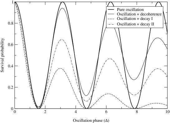
Figure 1: The qualitative effect of different damping signatures on the two-flavor neutrino survival probability as a function of the oscillation phase $\Delta$. The mixing used in this plot is maximal ($\theta=\pi/2$) and the damping parameters have been highly exaggerated. The scenario “Oscillation + decay I” corresponds to decay of both mass eigenstates with equal rates, whereas “Oscillation + decay II” corresponds to the second mass eigenstate decaying while the first mass eigenstate is stable.

From this figure, we clearly see how the wave packet decoherence simply corresponds to a damping of the oscillating term and the decay of all mass eigenstates corresponds to an overall damping of the undamped neutrino survival probability. For the case of only one decaying mass eigenstate, the probability converges towards the square of the content of the stable mass eigenstate in the initial neutrino flavor eigenstate.

3.2 Three-flavor electron-muon neutrino transitions

For a fixed neutrino oscillation channel, the damped neutrino oscillation probability Eq. (3) can be written more explicitly in terms of the mixing parameters and the mass squared differences. Below, we will use the standard notation for the leptonic mixing angles, i.e., $s_{ij}=\sin(\theta_{ij})$ and $c_{ij}=\cos(\theta_{ij})$. Then, for example, the $\nu_{e}$ survival probability $P_{ee}$ is given by

$$P_{ee} = c_{13}^{4}\left[D_{11}c_{12}^{4}+D_{22}s_{12}^{4}+\frac{1}{2}D_{21}\sin^{2}(2\theta_{12})\cos(2\Delta_{21})\right]$$ (32)

$$+\frac{1}{2}\sin^{2}(2\theta_{13})[D_{31}c_{12}^{2}\cos(2\Delta_{31})+D_{32}s_{12}^{2}\cos(2\Delta_{32})]+D_{33}s_{13}^{4},$$

which is dependent on all neutrino oscillation parameters except for $\theta_{23}$ and $\delta_{CP}$, while the probability $P_{e\mu}$ of oscillations into $\nu_{\mu}$ is given by

$$P_{e\mu} = \frac{1}{4}\sin^{2}(2\theta_{12})c_{23}^{2}[(D_{11}+D_{22})-2D_{21}\cos(2\Delta_{21})]$$ (33)

$$+\frac{1}{2}\sin(2\theta_{12})\sin(2\theta_{23})\{c_{\delta}[D_{11}c_{12}^{2}-D_{22}s_{12}^{2}-D_{21}\cos(2\theta_{12})\cos(2\Delta_{21})]$$

$$-D_{21}s_{\delta}\sin(2\Delta_{21})+D_{32}\cos(2\Delta_{32}-\delta_{CP})-D_{31}\cos(2\Delta_{31}-\delta_{CP})\}\,s_{13}$$

$$+s_{23}^{2}[D_{11}c_{12}^{4}+D_{22}s_{12}^{4}+D_{33}-2D_{31}s_{12}^{2}\cos(2\Delta_{31})-2D_{32}c_{12}^{2}\cos(2\Delta_{32})]\,s_{13}^{2}$$

$$+\frac{1}{4}\sin^{2}(2\theta_{12})[2D_{21}\cos(2\Delta_{21})-c_{23}^{2}(D_{11}+D_{22})]\,s_{13}^{2}+\mathcal{O}(s_{13}^{3}),$$

where $s_{\delta}\equiv\sin(\delta_{CP})$ and $c_{\delta}\equiv\cos(\delta_{CP})$. Furthermore, the $\nu_{\mu}$ survival probability can be computed to be of the form

$$P_{\mu\mu} = \frac{1}{2}\sin^{2}(2\theta_{23})[D_{32}c_{12}^{2}\cos(2\Delta_{32})+D_{31}s_{12}^{2}\cos(2\Delta_{31})]$$ (34)

$$+c_{23}^{4}\left[D_{11}s_{12}^{4}+D_{22}c_{12}^{4}+\frac{1}{2}D_{21}\sin^{2}(2\theta_{12})\cos(2\Delta_{21})\right]+D_{33}s_{23}^{4}$$

$$+c_{\delta}\sin(2\theta_{12})\sin(2\theta_{23})\left\{c_{23}^{2}\left[D_{11}s_{12}^{2}-D_{22}c_{12}^{2}+{D_{21}}\cos(2\theta_{12})\cos(2\Delta_{21})\right]\right.$$

$$\left.+s_{23}^{2}[D_{31}\cos(2\Delta_{31})-D_{32}\cos(2\Delta_{32})]\right\}\,s_{13}+\mathcal{O}(s_{13}^{2}).$$

Note that the probabilities $P_{e\mu}$ and $P_{\mu\mu}$ are series expansions in $s_{13}$, whereas the probability $P_{ee}$ is valid to all orders in $s_{13}$. The reason to use these expressions rather than the exact expressions is that, unless some further assumptions are made, the formulas for $P_{e\mu}$ and $P_{\mu\mu}$ are quite cumbersome.

The probability $P_{\mu e}$ can be obtained by making the transformation $\delta_{CP}\rightarrow-\delta_{CP}$ in the probability $P_{e\mu}$, i.e., $P_{\mu e}=P_{e\mu}(\delta_{CP}\rightarrow-\delta_{CP})$. Furthermore, in vacuum, the anti-neutrino oscillation probabilities can be obtain from the neutrino oscillation probabilities through the same transformation as above. Note that this is not true for neutrinos propagating in matter.

3.3 Probabilities for decoherence-like effects in experiments

For a decoherence-like damping effect, $D_{ii}=1$ for all $i$ and the relations

$$\sum_{\alpha=e,\mu,\tau}P_{\alpha\beta}=1\qquad{\rm and}\qquad\sum_{\beta=e,\mu,\tau}P_{\alpha\beta}=1$$ (35)

are still valid despite the presence of damping factors (i.e., no neutrinos are lost due to effects such as invisible decay, absorption, etc.). Note that, in the case of a decoherence-like damping effect, all neutrino oscillation probabilities can be constructed from $P_{ee}$, $P_{e\mu}$, and $P_{\mu\mu}$ due to the conservation of total probability given in Eq. (35).

It is interesting to observe what effect a decoherence-like damping could have on the neutrino oscillation probabilities for different experiments. Therefore, we will now study different kinds of neutrino oscillation experiments and make different approximations depending on the type of experiment to investigate what the main damping effects are.

Short-baseline reactor experiments

Short-baseline experiments, such as CHOOZ [66, 67] and Double-CHOOZ [68], are operated at the atmospheric oscillation maximum $\Delta_{31}\simeq\Delta_{32}=\mathcal{O}(1)$ in order to be sensitive to $\sin^{2}(2\theta_{13})$. The most interesting quantity is the $\bar{\nu}_{e}$ survival probability $P_{\bar{e}\bar{e}}$. For these experiments, it turns out (see Sec. 4) that it is important to keep all damping factors. As a result, the $\bar{\nu}_{e}$ survival probability is given by

$$P_{\bar{e}\bar{e}} = c_{13}^{4}\left\{1-\frac{1}{2}\sin^{2}(2\theta_{12})[1-D_{21}\cos(2\Delta_{21})]\right\}$$ (36)

$$+\frac{1}{2}\sin^{2}(2\theta_{13})[D_{31}c_{12}^{2}\cos(2\Delta_{31})+D_{32}s_{12}^{2}\cos(2\Delta_{32})]+s_{13}^{4}.$$

The most apparent feature of this equation is the term within the curly brackets, which has the form of the survival probability for a two-flavor neutrino damping scenario with $\theta=\theta_{12}$ and $\Delta=\Delta_{21}$. Therefore, even in the limit $\theta_{13}\rightarrow 0$ [close to the $\sin^{2}(2\theta_{13})$ sensitivity limit], the damping factor $D_{21}$ might be constrained by the contribution of the solar oscillation at low energies. Furthermore, in the limit $\Delta_{21}\rightarrow 0$ (or large $\theta_{13}$), $D_{21}$ is close to unity [cf., Eq. (7)] and $D_{31}\simeq D_{32}$ (this could be expected if $\Delta_{21}/\Delta_{31}\rightarrow 0$), then this expression will exactly mimic the two-flavor neutrino damping scenario with $\theta=\theta_{13}$ and $\Delta=\Delta_{31}=\Delta_{32}$. Thus, depending on which small number (the ratio of the mass squared differences or $s_{13}$) is the largest, two different two-flavor neutrino scenarios are obtained as expected from the non-damped case. If $\theta_{13}$ is relatively large (compared to the ratio of the mass squared differences), then the latter two-flavor case will apply. It is then interesting to note that the damping factor $D_{31}$, the neutrino source energy spectrum, and the cross-sections all have some energy dependence, which means that they can “emphasize” certain regions in the energy spectrum which are most sensitive to damping effects. If we assume that the total impact is strongest close to the oscillation maximum, then the damping effect will be misinterpreted as a smaller value of $\sin^{2}(2\theta_{13})$ [cf., Eq. (21), which will in both cases be closer to unity]. Therefore, as we will demonstrate, any such damping can fake a value of $\sin^{2}(2\theta_{13})$ which is smaller than the one that is provided by Nature.

Note that, for the case of wave packet decoherence, $D_{21}$, $D_{32}$, and $D_{31}$ are not independent [cf., Eq. (7)], which means that any of the terms in Eq. (36) could lead to information on the parameter $\sigma_{E}$.

Long-baseline reactor experiments

For long-baseline reactor experiments operated at the solar oscillation maximum $\Delta_{21}=\mathcal{O}(1)$, such as the KamLAND experiment [5, 6], the damping factors $D_{31}$ and $D_{32}$ of a decoherence-like scenario with $\xi>0$ are small, since the large mass squared difference makes the argument of the exponential functions in Eq. (4) large and negative. In addition, these two damping factors are attached to neutrino oscillations associated with the large phases $\Delta_{31}$ and $\Delta_{32}$ [see Eqs. (32)-(34)], which effectively average out. As a result of these two effects, the oscillating terms involving the third mass eigenstate can be safely set to zero. After some simplifications, the $\bar{\nu}_{e}$ survival probability $P_{\bar{e}\bar{e}}$ is found to be

$$P_{\bar{e}\bar{e}}=c_{13}^{4}\left\{1-\frac{1}{2}\sin^{2}(2\theta_{12})[1-D_{21}\cos(2\Delta_{21})]\right\}+s_{13}^{4}.$$ (37)

This expression is clearly of the familiar form $P_{\bar{e}\bar{e}}=c_{13}^{4}P_{\bar{e}\bar{e}}^{\rm 2f}+s_{13}^{4}$, where $P_{\bar{e}\bar{e}}^{\rm 2f}$ is the damped two-flavor $\bar{\nu}_{e}$ survival probability with $\theta=\theta_{12}$ and $\Delta=\Delta_{21}$, which is also obtained in the non-damped case when averaging over the fast oscillations [cf. Eq. (36)]. For the case of wave packet decoherence, we know from Eq. (7) that the parameter $\sigma_{E}$ could be constrained by either of these two equations. Since this parameter is experiment dependent, one could argue that one should obtain some limits from the KamLAND experiment, because the reactor experiments are very similar in source and detector (see, e.g., Ref. [69]). However, it should be noted that KamLAND has a rather weak precision on the corresponding $\theta_{12}$ measurement because of normalization uncertainties. Since a decoherence contribution would appear at low energies, the data set in Ref. [6] does not seem to be very restrictive for the parameter $\sigma_{E}$.

Beam experiments

For beam experiments, such as superbeams, beta-beams or neutrino factories, one may assume $\Delta_{21}\simeq 0$ as a first approximation if one wants to be sensitive to $\sin^{2}(2\theta_{13})$, since, at the energies and baseline lengths involved, the low-frequency neutrino oscillations do not have enough time to evolve. In the case of $\xi>0$, this also implies that $D_{12}=1$ and $D\equiv D_{32}=D_{31}$ to a good approximation. From these assumptions, it follows that

$$P_{e\mu} = 2s_{23}^{2}[1-D\cos(2\Delta)]\,s_{13}^{2}+\mathcal{O}(s_{13}^{3}),$$ (38)

$$P_{\mu\mu} = 1-\frac{1}{2}\sin^{2}(2\theta_{23})[1-D\cos(2\Delta)]+\mathcal{O}(s_{13}^{2}),$$ (39)

where $\Delta\equiv\Delta_{32}=\Delta_{31}$. Note that the probability $P_{e\mu}$ is correct up to $\mathcal{O}(s_{13}^{3})$ [as compared with Eq. (33), which is only valid up to $\mathcal{O}(s_{13}^{2})$], this is one of the cases where the assumptions made simplifies the $s_{13}^{2}$ term in this probability. Both of the above equations show obvious similarities with the cases of damped two-flavor neutrino oscillations. For $P_{e\mu}$ we have an approximate two-flavor neutrino scenario with $s^{2}c^{2}=s_{23}^{2}s_{13}^{2}$ and $P_{\mu\mu}$ is a pure two-flavor neutrino formula with $\theta=\theta_{23}$ up to the corrections of order $s_{13}^{2}$. Since the disappearance channel $P_{\mu\mu}$ at a beam experiment is supposed to have extremely good statistics, $D$ will be strongly constrained by this channel. Note that the damping in $P_{\mu\mu}$ qualitatively behaves as the one in Eq. (21), i.e., the damped probability might be larger or smaller than the undamped probability depending on the position relative to the oscillation maximum $E_{\mathrm{max}}$.

3.4 Probabilities for decay-like effects in experiments

If $\xi=0$ and $\alpha_{ii}\neq 0$, then $D_{ii}\neq 1$ and Eq. (35) will not hold. We define any effect of this kind to be “probability violating”. As mentioned in the two-flavor neutrino discussion, a very interesting special case of the probability violating effects is the case of a decay-like effect. The neutrino oscillation probabilities for decay-like effects corresponding to the ones given for decoherence-like effects are listed below.

Short-baseline reactor experiments

For the short-baseline reactor experiments, we obtain the $\bar{\nu}_{e}$ survival probability as

$$P_{\bar{e}\bar{e}} = c_{13}^{4}\left\{(A_{1}c_{12}^{2}+A_{2}s_{12}^{2})^{2}-A_{1}A_{2}\sin^{2}(2\theta_{12})\sin^{2}(\Delta_{21})\right\}$$ (40)

$$+A_{3}s_{13}^{2}\{A_{3}s_{13}^{2}+2c_{13}^{2}[A_{1}c_{12}^{2}\cos(2\Delta_{31})+A_{2}s_{12}^{2}\cos(2\Delta_{32})]\}.$$

Again, as in the case of decoherence-like damping, the expression within the curly brackets is of a two-flavor form with $\theta=\theta_{12}$ and $\Delta=\Delta_{12}$. In the limit when $\sin^{2}(2\theta_{13})$ is large and we ignore the solar oscillations, we obtain the two-flavor neutrino scenario

$$P_{\bar{e}\bar{e}}=A^{2}\left\{(c_{13}^{2}+\kappa s_{13}^{2})^{2}-\kappa\sin^{2}(2\theta_{13})\sin^{2}(2\Delta)\right\}$$ (41)

only if we assume that $A_{1}=A_{2}=A$, where $\Delta=\Delta_{31}=\Delta_{32}$ and $\kappa=A_{3}/A$.

Long-baseline reactor experiments

Assuming that the fast neutrino oscillations average out, the $\bar{\nu}_{e}$ survival probability is given by

$$P_{\bar{e}\bar{e}}=c_{13}^{4}P_{\bar{e}\bar{e}}^{\rm 2f}+A_{3}^{2}s_{13}^{4},$$ (42)

where $P_{\bar{e}\bar{e}}^{\rm 2f}$ is the two-flavor decay-like $\bar{\nu}_{e}$ survival probability with $\theta=\theta_{12}$ and $\Delta=\Delta_{21}$ [cf., Eq. (37)]. In this expression, the $s_{13}^{4}$ term is also damped, which does not apply in a decoherence-like scenario.

Beam experiments

When the assumptions $\Delta_{21}\simeq 0$ and $A=A_{1}=A_{2}$ (which could be expected in a decay scenario where $m_{1}=m_{2}$) are made, the neutrino oscillation probabilities that are relevant for beam experiments become

$$P_{e\mu} = A^{2}s_{23}^{2}[1+\kappa^{2}-2\kappa\cos(2\Delta)]\,s_{13}^{2}+\mathcal{O}(s_{13}^{3}),$$ (43)

$$P_{\mu\mu} = A^{2}\left[(c_{23}^{2}+\kappa s_{23}^{2})^{2}-\kappa\sin^{2}(2\theta_{23})\sin^{2}(\Delta)\right]+\mathcal{O}(s_{13}^{2}),$$ (44)

where $\kappa\equiv A_{3}/A$ and $\Delta\equiv\Delta_{32}=\Delta_{31}$. These probabilities mimic decay-like two-flavor probabilities just as the corresponding decoherence-like effects mimic decoherence-like two-flavor probabilities to leading order in $s_{13}$.

4 Application I: Faking a small $\boldsymbol{\sin^{2}(2\theta_{13})}$ at reactor experiments by decoherence-like effects

In this section, we demonstrate the possible effects of damping at a simple example using a full numerical simulation. Let us only consider the case of intrinsic wave packet decoherence, which is very interesting from the point of view that it is a “standard” effect in any realistic neutrino oscillation treatment. However, similar effects could occur from related signatures, such as quantum decoherence. As experiments, one could, in principle, consider all classes of experiments in order to investigate decoherence signals. New reactor experiments with near and far detectors [70, 71] are candidates for “clean” measurements of $\sin^{2}(2\theta_{13})$, i.e., they are specifically designed to search for a $\sin^{2}(2\theta_{13})$ signal. As we have discussed in Sec. 3.3, an interesting decoherence-like effect at such an experiment would be a derived value of $\sin^{2}(2\theta_{13})$ which is smaller than the value provided by Nature. In this case, the CHOOZ bound might actually be too strong and the interpretation of new reactor experiments might be wrong.

If we assume that there is an intrinsic loss of coherence, then the reactor $\bar{\nu}_{e}$ survival probability $P_{\bar{e}\bar{e}}$ will be given by Eq. (36). In order to illustrate the decoherence effect, we show in Fig. 2 $P_{\bar{e}\bar{e}}$ and the corresponding event rates for the experiment Reactor-I from Ref. [71] (full analysis range shown).

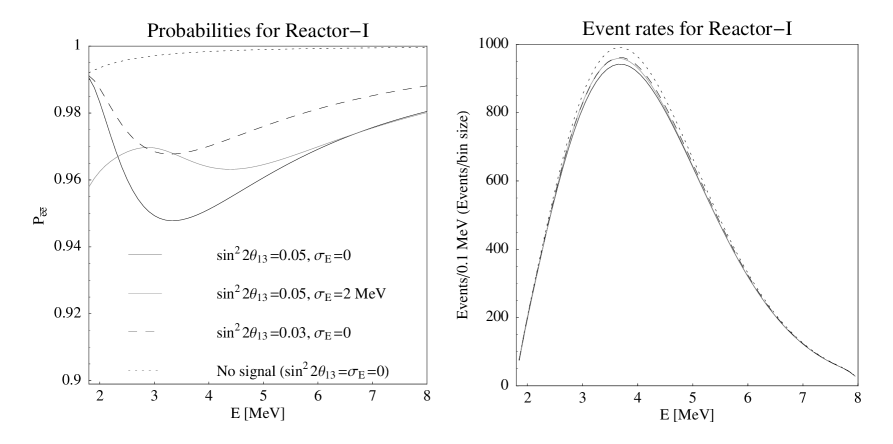
Figure 2: The neutrino oscillation probability $P_{\bar{e}\bar{e}}$ (left) and event rates (right) for the experiment Reactor-I from Ref. [71] in the analysis range. For the simulated parameter values, we use $\Delta m_{31}^{2}=2.5\cdot 10^{-3}\,\mathrm{eV}^{2}$, $\Delta m_{21}^{2}=8.2\cdot 10^{-5}\,\mathrm{eV}^{2}$, $\sin^{2}2\theta_{12}=0.83$, $\sin^{2}2\theta_{23}=1$, $\delta_{CP}=0$ [72, 73, 74, 22] and the values for $\sin^{2}(2\theta_{13})$ and $\sigma_{E}$ as given in the left plot.

The different curves correspond to the non-oscillatory case as well as different combinations of $\sin^{2}(2\theta_{13})$ and $\sigma_{E}$. As one can observe, the two cases $\sin^{2}(2\theta_{13})$ large and decoherence [$\sin^{2}(2\theta_{13})=0.05$ and $\sigma_{E}=2\,\mathrm{MeV}$] and $\sin^{2}(2\theta_{13})$ small and no decoherence [$\sin^{2}(2\theta_{13})=0.03$ and $\sigma_{E}=0$] correspond, especially in the event rate plot, very well to each other [as compared to the other two cases of no oscillations and large $\sin^{2}(2\theta_{13})$ only]. This means that the decoherence effect can mimic a smaller value of $\sin^{2}(2\theta_{13})$ than what is provided by Nature. Note that in the probability plot, there is a significant contribution from loss of coherence in the solar terms for low energies. As we will see later, this contribution can limit the decoherence effects even for no $\sin^{2}(2\theta_{13})$ signal. In addition, the damped neutrino oscillation probability is larger than the undamped one in the range discussed after Eq. (21), where the oscillation maximum is here at about $E_{\mathrm{max}}\simeq 3.4\,\mathrm{MeV}$.

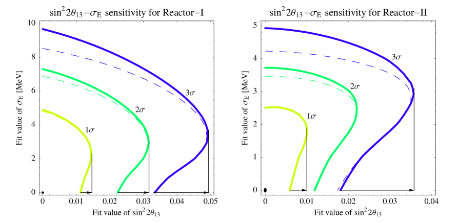
Figure 3: Simultaneous sensitivity to $\sin^{2}(2\theta_{13})$ and $\sigma_{E}$ for the experiments Reactor-I (left) and Reactor-II (right) from Ref. [71] (curves shown for 1 d.o.f). For the simulated parameter values, we use $\sin^{2}(2\theta_{13})=0$, $\sigma_{E}=0$, and the other values as in Fig. 2. For the thick solid curves, the unshown fit parameter values are marginalized over, where post-KamLAND external precisions of 10 % on each $\Delta m_{21}^{2}$ and $\theta_{12}$ [75, 76] are imposed along with an external error of 10 % for $\Delta m_{31}^{2}$ obtained from the superbeams is assumed. For the thin dashed curves, the unshown fit parameter values are fixed (no correlations). For the numerical analysis, an extended version of the GLoBES software [77] is used. The arrows indicate the shift of the $\sin^{2}(2\theta_{13})$ sensitivity limit if one assumes $\sigma_{E}$ as a free parameter.

In order to illustrate the effect for a complete analysis, we show in Fig. 3 the simultaneous sensitivity to $\sin^{2}(2\theta_{13})$ and $\sigma_{E}$ for Reactor-I ($\mathcal{L}=400\,\mathrm{t\,GW\,yr}$) and Reactor-II ($\mathcal{L}=8\,000\,\mathrm{t\,GW\,yr}$) from Ref. [71] (1 d.o.f.) using an extended version of the GLoBES software [77]. In this figure, $\sigma_{E}$ is assumed to be a free (fit) parameter that has to be measured by the experiment. Therefore, without additional knowledge, the $\sin^{2}(2\theta_{13})$ sensitivity limit is obtained as a projection of the curves onto the $\sin^{2}(2\theta_{13})$-axis. Since the $\sin^{2}(2\theta_{13})$ sensitivity limit for no decoherence effects is the one for $\sigma_{E}=0$, the arrows indicate the shift of this limit by the unknown $\sigma_{E}$. This means, for example, that the sensitivity limit becomes about 50 % to 100 % worse than that for the actual $\sigma_{E}\equiv 0$, since the decoherence mimics a smaller value of $\sin^{2}(2\theta_{13})$ than what is provided by Nature. Similar results to the left plot are obtained for the proposed Double-CHOOZ experiment [68]. Note that the correlation between $\sin^{2}(2\theta_{13})$ and $\sigma_{E}$ affects the $\sin^{2}(2\theta_{13})$ sensitivity (projection onto the horizontal axis), but not the $\sigma_{E}$ sensitivity (projection onto the vertical axis). The latter is correlated with the other neutrino oscillation parameters (especially the solar parameters), as one can read off from the difference between the solid and dashed curves. For the $\sigma_{E}$ sensitivity, one obtains $\sigma_{E}\lesssim 10\,\mathrm{MeV}$ (Reactor-I) and $\sigma_{E}\lesssim 5\,\mathrm{MeV}$ (Reactor-II) at the $3\sigma$ confidence level. As one can observe from the left plot of Fig. 2, there is some contribution of the solar oscillation averaging to the decoherence effect at low energies. In fact, this is the reason why one can constrain $\sigma_{E}$ even for $\sin^{2}(2\theta_{13})\equiv 0$, since in the decoherence effect, the atmospheric oscillations are suppressed by the oscillation amplitude $\sin^{2}(2\theta_{13})$. Obviously, this solar decoherence effect determines the upper bound for $\sigma_{E}$, which means that the $\sigma_{E}$ sensitivity is limited by the knowledge on the solar oscillation parameters [cf., Eq. (36)].

As we have discussed in Sec. 2, $\sigma_{E}$ might be an experiment dependent parameter related to the production and detection processes. Instead of deriving bounds for this parameter from reactor experiments, one can estimate from Fig. 3 that one has to constrain $\sigma_{E}$ better than to about $\sigma_{E}\lesssim 0.5\,\mathrm{MeV}$ in order not to have a significant deterioration of the $\sin^{2}(2\theta_{13})$ sensitivity limit. In addition, in order to exclude an experiment dependent effect, it is highly recommendable to measure the same quantity with different techniques such as $\sin^{2}(2\theta_{13})$ with both reactor experiments and superbeams.

5 Application II: Testing and disentangling damping signatures at neutrino factories

If we want to constrain the model parameters in Table 1 and to test the different models against each other, then we will need to choose a high-precision instrument to test these tiny effects. Therefore, we investigate the potential of a neutrino factory. In particular, the muon neutrino disappearance channel $\nu_{\mu}\rightarrow\nu_{\mu}$ at a neutrino factory has very good statistics and the impact of neutrino oscillation parameter correlations other than with $\Delta m_{31}^{2}$ and $\theta_{23}$ is very small. Thus, we will mainly focus on this disappearance channel, but include the appearance information in the full analysis and demonstrate how the value of $\sin^{2}(2\theta_{13})$ would influence the effects. Since our exponential damping model is not directly comparable to other approaches in the literature, we put a major emphasis on the identification problem of a non-standard contribution: If we actually observe something unexpected, how well can we determine what sort of effect this actually is? In the simplest case, this means that we test a signature against the standard (no damping) scenario giving us limits for the parameters. Since it is almost impossible to include the correlations among all parameters, we choose to use $\alpha_{ij}=\alpha$ independent of $i$ and $j$ in this section in order to drastically reduce the number of parameters. This means that we now have to deal with eight correlated parameters (six neutrino oscillation parameters, the matter density, and the parameter $\alpha$). We have motivated this choice at the end of Sec. 2.1 and, for individual cases, in Sec. 2.3.

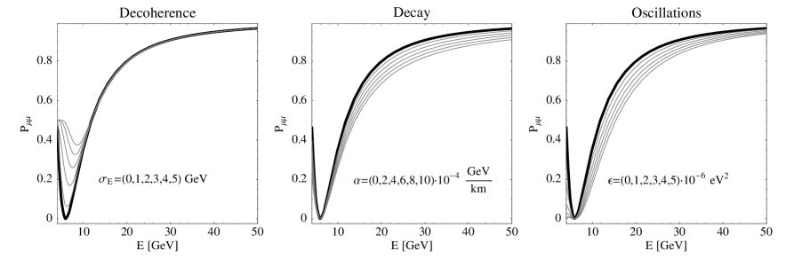
Figure 4: Contributions of the first three different damping signatures from Table 1 to the disappearance probability $P_{\mu\mu}$ as function of the neutrino energy. Here $L=3\,000\,\mathrm{km}$ and the neutrino oscillation parameters as in Fig. 2 with $\sin^{2}(2\theta_{13})=0$ are used. The parameters for the non-standard effects are given in the plots, where zero corresponds to the thick curves (oscillations only) and larger values correspond to curves further off the zero curve. The energy range corresponds to the analysis range of the $50\,\mathrm{GeV}$ neutrino factory NuFact-II from Ref. [78].

Before we come to the results of a complete simulation, let us illustrate the spectral behavior (energy dependence) of the neutrino oscillation probability $P_{\mu\mu}$ in Fig. 4 for some characteristic examples. Earlier in Sec. 3 we have already discussed that there are two general interesting cases: Either only the oscillatory terms are damped or all terms are damped. In Fig. 4, we can clearly identify this difference between the decoherence-like and the other two damping models (decay and oscillations). In all the shown cases (for which $\gamma>0$), the relative importance of the damping increases as the energy decreases. However, since also the neutrino oscillation probability drops with lower energies, the absolute size of the effect is determined by the ratio of signature versus probability effect for low energies. In addition, cross-section and flux will disfavor low energies, which means that the low-energy effects become even harder to identify. This makes the wave packet decoherence scenario most difficult to test, since the $E^{-4}$ dependence in the exponent strongly favors low energies. However, it might be most easily distinguished from the decay and oscillation damping scenarios because of its unique signature. As we have discussed after Eq. (21) [which also holds for the similar Eq. (39)], it is a characteristic feature of decoherence-like signatures that they cross the undamped curve at $2E_{\mathrm{max}}/3$ and $2E_{\mathrm{max}}$, which here evaluate to $4\,\mathrm{GeV}$ (outside of the analysis range) and $12\,\mathrm{GeV}$. In Fig. 4 (left panel), this effect is hardly observable because of the $E^{-4}$ energy dependence, but the quantum decoherence motivated case “Quantum decoherence II” from Table 1 clearly shows this behavior because of an $E^{-2}$ energy dependence. As far as the other two signatures are concerned, the decay damping has a linear energy dependence in the exponent as opposed to the quadratic one for the oscillation damping scenario. Therefore, one has the strongest high-energy effect for the decay damping scenario.

	Simulated damping signature
	Decoherence	Decay	Oscillations	Absorption	Q. decoh. I	Q. decoh. II
Fit signature	$\frac{\sigma_{E}}{\mathrm{GeV}}$ $\gtrsim$	$\frac{\alpha}{10^{-5}\,\mathrm{\frac{GeV}{km}}}\gtrsim$	$\frac{\epsilon}{10^{-7}\,\mathrm{eV}^{4}}\gtrsim$	$\frac{\alpha}{\frac{10^{-8}}{\mathrm{GeV\,km}}}\,\gtrsim$	$\frac{\alpha}{\frac{10^{-10}}{\mathrm{GeV^{2}\,km}}}\gtrsim$	$\frac{\kappa}{\frac{10^{24}}{\mathrm{eV}^{2}}}\gtrsim$
No damping	1.7 (2.8)	4.3 (7.2)	5.1 (8.3)	1.9 (3.1)	4.1 (6.8)	2.0 (3.6)
Decoherence	-	4.3 (7.2)	5.1 (8.3)	1.9 (3.1)	4.1 (6.8)	2.0 (3.6)
Decay	1.7 (2.8)	-	6.3 (10)	3.4 (5.7)	6.0 (10)	2.6 (5.1)
Oscillations	1.7 (2.8)	5.8 (9.8)	-	1.9 (3.2)	4.1 (6.9)	13 (17)
Absorption	1.7 (2.8)	7.8 (13)	5.2 (8.5)	-	24 (40)	2.1 (3.8)
Q. decoh. I	1.7 (2.8)	6.3 (11)	5.1 (8.3)	11 (19)	-	2.1 (3.7)
Q. decoh. II	1.7 (2.8)	4.3 (7.2)	5.1 (8.3)	1.9 (3.1)	4.1 (6.8)	-
All models	1.7 (2.8)	7.8 (13)	6.3 (10)	11 (19)	24 (40)	13 (17)

Table 3: Parameter sensitivity limits for which the simulated models (in columns) from Table 1 could be distinguished from the fit models (in rows) at the $3\sigma$ ($5\sigma$) confidence level (for the experiment simulation NuFact-II from Ref. [78]). For example, decoherence could be established against all models (including standard oscillations) for the simulated $\sigma_{E}\gtrsim 1.7\,\mathrm{GeV}$. For the simulated neutrino oscillation parameter values, we use the same values as in Fig. 2 and $\sin^{2}(2\theta_{13})=0$ as given in the column captions. The fit parameter values (including the model parameter $\alpha$) are marginalized over. The row “no damping” corresponds to the standard neutrino oscillation scenario, i.e., it corresponds to the upper bounds for the parameters assuming that there is only one non-standard effect. The row “All models” corresponds to the most conservative case, i.e., it is an estimate for how well one can establish the model against all of the other shown models.

In order to test the different models against each other, we use a modified version of the GLoBES software [77] and the neutrino factory setup NuFact-II from Ref. [78]. This neutrino factory uses a $50\,\mathrm{kt}$ magnetized iron detector, $4\,\mathrm{year}$ of running time in each polarity, and $4\,\mathrm{MW}$ target power (corresponding to $5.3\cdot 10^{20}$ useful muon decays per year). For a fixed set of simulated parameter values including the simulated damping parameter $\alpha$, we marginalize over the fit neutrino oscillation parameters including the fit damping parameter. Due to the complexity of the parameter space, we assume that the $\mathrm{sgn}(\Delta m_{31}^{2})$-degeneracy has been resolved by this time. We define the sensitivity limit to $\alpha$ as the threshold above which the simulated damping model could be distinguished from the fit damping model. Thus, if the damping mechanism is really there, then the damping parameter $\alpha$ has to be above this threshold in order to establish the model against the fit model with the given experiment. In particular, we include the fit damping model “no damping”, which corresponds to the standard neutrino oscillation case. For the simulation, we impose external precisions of 10 % on each $\theta_{12}$ and $\Delta m_{21}^{2}$ [75, 76]. In addition, we assume a constant matter density profile with 5 % uncertainty, which takes into account matter density uncertainties as well as matter density profile effects [79, 80, 81]. However, we assume that the neutrino factory itself measures $\Delta m_{31}^{2}$ and $\theta_{23}$ with its disappearance channel, i.e., we do not impose an external precision on these parameters.

The resulting sensitivity limits of this analysis are shown in Table 3, where the columns correspond to the simulated models and the rows correspond to the fit models. These results are computed for $\sin^{2}(2\theta_{13})=0$. It turns out that for a simulated value of $\sin^{2}(2\theta_{13})$ close to the CHOOZ bound $\sin^{2}(2\theta_{13})\simeq 0.1$, the limits on $\alpha$ would improve up to about 30 % [depending on model and value of $\sin^{2}(2\theta_{13})$] because of the additional contribution from the appearance signal. Let us first of all discuss the resulting sensitivities against the standard neutrino oscillation scenario for some simple cases. For decoherence, the obtained numbers indeed correspond very well to the energy resolution of the detector, which is about 15 % of the neutrino energy, i.e., $1.5\,\mathrm{GeV}$ for a neutrino energy of $E=10\,\mathrm{GeV}$, where the major effect takes place (cf., Fig. 4, left plot). Since the neutrino oscillation probability changes sufficiently fast in this region, the measurement is limited by the energy resolution of the detector. In the wave packet approach, the bound against the “no damping” model $\sigma_{E}\lesssim 1.67\,\mathrm{GeV}$ translates into $\sigma_{x}\gtrsim 6\cdot 10^{-17}\,\mathrm{m}$. This rather small number (sub-nucleon size) means that the bound is not very useful for wave packet decoherence, since it is virtually impossible to create such sharply peaked wave packets. However, there might be other energy averaging effects that can be constrained. For decay, we obtain a limit, against the standard model, which is comparable to the current neutrino lifetime limit for $m_{3}$. Note that we have included all correlations with the neutrino oscillation parameters in this limit. However, the limit would be a factor of two weaker if we considered only decay of $m_{3}$ instead of all mass eigenstates. Since there are quite strong bounds on the $m_{1}$ and $m_{2}$ lifetimes from supernova and solar neutrino observations, this factor of two difference should be a very good approximation for the actual limit. For the oscillation signature, the obtained limits are of the order of magnitude $5\cdot 10^{-7}\,\mathrm{eV}^{2}$, which corresponds to $(\Delta m_{43}^{2})^{2}$ times the active-sterile mixing in our estimate for a possible mass scheme (cf., Sec. 2.3). Considering the $\Delta m_{43}^{2}$ dependence, this is in fact not a very strong bound. However, note that we have taken into account the full parameter correlation, i.e., this effect could not come from $\sin^{2}(2\theta_{13})$ or any other standard parameter.

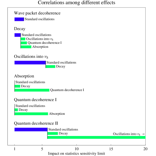
Figure 5: The impact of different correlations on the statistics (and systematics) sensitivity limit of the model dependent parameter $\alpha$ ($3\sigma$), where the horizontal axis represents multiples of the statistics (and systematics) sensitivity limit. The group captions refer to the simulated models and the bar labels to the fit models, where only the fit models are shown which affect the sensitivity limit more than by 5 %. The dark bars represent the correlations with the neutrino oscillation parameters (fit parameter $\alpha=0$ fixed) and the light bars indicate the additional change if the model specific fit parameter $\alpha$ is marginalized over. The lowest light bar extends to $37$.

In order to discuss the general identification problem among different damping signatures, some information can be obtained from Table 3. In addition, in Fig. 5 we show the impact of the correlations with the standard neutrino oscillation parameters (dark bars) as well as the additional correlation with the fit model parameter $\alpha$ (light bars) on the $\alpha$ sensitivity limit for the simulated models from Table 1. The horizontal axis shows the ratio of the $\alpha$ sensitivity limit including correlations to the one from statistics and systematics only (which corresponds to $1$), where we only include fit models with relevant model parameter contributions. Two models are highly correlated if a possible signature in one model can be compensated by a change of parameter(s) in the other. Since we include the standard neutrino oscillation scenario in all models, a small change in the fit neutrino oscillation parameters might also compensate a damping signature within the measurement precision of the experiment. Therefore, we include for all signatures the standard neutrino oscillation parameter correlation as dark bars, i.e., the dark bars represent the fit against the standard neutrino oscillation scenario (for fixed fit parameter $\alpha$), and the light bars are a measure for the additional problem to distinguish a non-standard signature from the ones of other possible non-standard models. The interpretation of these bars is as follows: The dark bars reflect the limit (right edges) for $\alpha$ (as multiple of the statistics limit) beyond which the non-standard signature could be distinguished from the standard neutrino oscillation case at the $3\sigma$ confidence level. However, if $\alpha$ should be within one of the light bar ranges, then it could not be uniquely identified, since it could also well be the non-standard signature corresponding to this bar. From Fig. 5, we make a number of interesting observations:

• Signatures which have negative $\gamma$’s (Absorption and Quantum decoherence I) are almost not affected by correlations with the neutrino oscillation parameters, i.e., they cannot be explained by different neutrino oscillation parameter values. In these cases, the spectrum is more suppressed for large values of $E$ than for small values, which means that the signature behaves unlike an oscillation signature corresponding to $\gamma=2$. However, it is difficult to identify which of these models is realized.

• Signatures with $\gamma=2$ (Oscillations into $\nu_{s}$ and Quantum decoherence II) are highly affected by correlations with the standard neutrino oscillation parameters, since the signatures have an energy dependence similar to the oscillation signature. Similar signatures, such as decay, can enhance this correlation.

• Unique signatures (Wave packet decoherence and Neutrino decay) can easily be distinguished from all the other models. Although there could be some correlations with similar signatures for neutrino decay, the absolute impact on the $\alpha$ sensitivity limit is comparatively small (up to a factor of three).

6 Summary and conclusions

We have introduced exponential damping factors in the neutrino oscillation probabilities, which lead to distinctive signatures, i.e., energy dependent damping effects in the energy spectrum. These damping factors are one approach to test non-oscillation effects on the neutrino oscillation probability level. They can be motivated by many different models such as intrinsic wave packet decoherence, neutrino decay, oscillations into sterile neutrinos, neutrino absorption, quantum decoherence, etc.. They describe the second order contributions of small possible “non-standard” corrections to the three-flavor neutrino oscillation framework (in vacuum as well as in matter) on a rather abstract level. As opposed to tests of probability conservation, the damping factors can, in addition, describe a damping of the oscillating terms (which preserves the total probability) as well as they imply, by their energy dependence, some information on the type of effect. We have demonstrated how damping factors can modify the neutrino oscillation probabilities relevant for future high-precision short- and long-baseline experiments, since these experiments might be most sensitive to very small spectral effects.

As one application, we have shown that decoherence-like damping signatures can severely modify the interpretation of experiments, where we have chosen wave packet decoherence damping at new short-baseline reactor experiments as an example. In this case, two competing small effects, namely the effect of a non-zero value of $\sin^{2}(2\theta_{13})$ and a damping contribution, might be mixed up. In particular, the damping could fake a value of $\sin^{2}(2\theta_{13})$ which is much smaller than the value provided by Nature. Such a $\sin^{2}(2\theta_{13})$ suppression effect can either be intrinsic (such as quantum decoherence), experiment dependent (such as some averaging effect not taken into account), or both (such as wave packet decoherence related to the production and detection processes). Intrinsic effects will be observable by all types of experiments, which means that there are very stringent limits available from existing data as well as future experiments will test the consistency of the picture. On the other hand, experiment dependent effects can only be checked by complementary techniques measuring the same quantity. One such complementary pair has, in the past, been the solar and long-baseline reactor experiments. In the future, it will therefore be very important to measure $\sin^{2}(2\theta_{13})$ by reactor experiments and superbeams as complementary techniques, since one of them alone could fail for such experiment dependent effects. Eventually, the LSND experiment could be a strong hint for such an experiment dependent effect if it is rejected by the MiniBooNE experiment.

One of the most interesting features of damping signatures are their characteristic spectral (energy) dependencies, which can act as a “fingerprint” for many sources of non-oscillation effects. For example, specific signatures could point to new interesting physics beyond the standard model. We have therefore discussed how large the effects from different damping signatures have to be in order to be identified and how well these damping signatures could be distinguished for the example of neutrino factories. In some cases, such damping signatures can be compensated by a shift of the neutrino oscillation parameters, which means that given such a damping effect, it is quite likely to obtain an erroneous determination of these parameters. However, if the damping effects are strong enough, then an establishment of non-oscillation effects will be possible. Once such a damping effect is established, it will be very interesting to know from which non-standard mechanism it actually arises. Given this question of the identification problem, we have found that signatures with a damping similar to $\exp(-\alpha L^{\beta}/E^{\gamma})$, $\gamma=1,2,\ldots$ are strongly correlated (peaking at $\gamma=2$) with the standard neutrino oscillation parameters, i.e., it is difficult to distinguish them from small adjustments in the neutrino oscillation parameters. However, damping signatures similar to $\exp(-\alpha L^{\beta}E^{2})$ can be very easily disentangled from the neutrino oscillation parameters, but it is difficult to distinguish them from each other. It is also extremely difficult to establish a damping of the oscillations against a damping of the probabilities with the same spectral index $\gamma$ because of the correlations with the neutrino oscillation parameters.

Finally, we conclude that spectral tests of damping signatures in neutrino oscillation probabilities are an important test of the consistency of the three-flavor neutrino oscillation picture. If any deviation from this picture is found, then the most important question will be what sort of effect we are dealing with. Exactly this information could be provided by the spectral dependence of the damping signature, which means that this approach could be an important test of physics beyond the standard model.

Acknowledgments

We would like to thank John Bahcall, Manfred Lindner, and Thomas Schwetz for useful discussions.

T.O. and W.W. would like to thank the IAS and the KTH respectively for the warm hospitality and the financial support during their respective research visits.

This work was supported by the Royal Swedish Academy of Sciences (KVA), the Swedish Research Council (Vetenskapsrådet), Contract Nos. 621-2001-1611, 621-2002-3577, the Göran Gustafsson Foundation, the Magnus Bergvall Foundation, the W. M. Keck Foundation, and NSF grant PHY-0070928.

References

- [1] Super-Kamiokande, Y. Fukuda et al., Evidence for oscillation of atmospheric neutrinos, Phys. Rev. Lett. 81 (1998), 1562, hep-ex/9807003.
- [2] SNO, Q. R. Ahmad et al., Direct evidence for neutrino flavor transformation from neutral-current interactions in the Sudbury Neutrino Observatory, Phys. Rev. Lett. 89 (2002), 011301, nucl-ex/0204008.
- [3] SNO, S. N. Ahmed et al., Measurement of the total active 8B solar neutrino flux at the Sudbury Neutrino Observatory with enhanced neutral current sensitivity, Phys. Rev. Lett. 92 (2004), 181301, nucl-ex/0309004.
- [4] K2K, M. H. Ahn et al., Indications of neutrino oscillation in a 250-km long-baseline experiment, Phys. Rev. Lett. 90 (2003), 041801, hep-ex/0212007.
- [5] KamLAND, K. Eguchi et al., First results from KamLAND: Evidence for reactor anti- neutrino disappearance, Phys. Rev. Lett. 90 (2003), 021802, hep-ex/0212021.
- [6] KamLAND, T. Araki et al., Measurement of neutrino oscillation with KamLAND: Evidence of spectral distortion, hep-ex/0406035.
- [7] Super-Kamiokande, Y. Ashie et al., Evidence for an oscillatory signature in atmospheric neutrino oscillation, Phys. Rev. Lett. 93 (2004), 101801, hep-ex/0404034.
- [8] C. Giunti and C. W. Kim, Coherence of neutrino oscillations in the wave packet approach, Phys. Rev. D58 (1998), 017301, hep-ph/9711363.
- [9] C. Giunti, Coherence and wave packets in neutrino oscillations, Found. Phys. Lett. 17 (2004), 103, hep-ph/0302026.
- [10] C. Giunti, C. W. Kim, and U. W. Lee, Coherence of neutrino oscillations in vacuum and matter in the wave packet treatment, Phys. Lett. B274 (1992), 87.
- [11] W. Grimus, P. Stockinger, and S. Mohanty, The field-theoretical approach to coherence in neutrino oscillations, Phys. Rev. D59 (1999), 013011, hep-ph/9807442.
- [12] C. Y. Cardall, Coherence of neutrino flavor mixing in quantum field theory, Phys. Rev. D61 (2000), 073006, hep-ph/9909332.
- [13] J. N. Bahcall, N. Cabibbo, and A. Yahil, Are neutrinos stable particles?, Phys. Rev. Lett. 28 (1972), 316.
- [14] V. Barger, W. Y. Keung, and S. Pakvasa, Majoron emission by neutrinos, Phys. Rev. D25 (1982), 907.
- [15] J. W. F. Valle, Fast neutrino decay in horizontal Majoron models, Phys. Lett. B131 (1983), 87.
- [16] V. Barger, J. G. Learned, S. Pakvasa, and T. J. Weiler, Neutrino decay as an explanation of atmospheric neutrino observations, Phys. Rev. Lett. 82 (1999), 2640, astro-ph/9810121.
- [17] S. Pakvasa, Do neutrinos decay?, AIP Conf. Proc. 542 (2000), 99, hep-ph/0004077.
- [18] V. Barger et al., Neutrino decay and atmospheric neutrinos, Phys. Lett. B462 (1999), 109, hep-ph/9907421.
- [19] M. Lindner, T. Ohlsson, and W. Winter, A combined treatment of neutrino decay and neutrino oscillations, Nucl. Phys. B607 (2001), 326, hep-ph/0103170.
- [20] M. Lindner, T. Ohlsson, and W. Winter, Decays of supernova neutrinos, Nucl. Phys. B622 (2002), 429, astro-ph/0105309.
- [21] A. Strumia, Interpreting the LSND anomaly: Sterile neutrinos or CPT-violation or …?, Phys. Lett. B539 (2002), 91, hep-ph/0201134.
- [22] M. Maltoni, T. Schwetz, M. A. Tortola, and J. W. F. Valle, Status of global fits to neutrino oscillations, New J. Phys. 6 (2004), 122, hep-ph/0405172.
- [23] A. De Rújula, S. L. Glashow, R. R. Wilson, and G. Charpak, Neutrino exploration of the Earth, Phys. Rept. 99 (1983), 341.
- [24] E. Lisi, A. Marrone, and D. Montanino, Probing possible decoherence effects in atmospheric neutrino oscillations, Phys. Rev. Lett. 85 (2000), 1166, hep-ph/0002053, and references therein.
- [25] F. Benatti and R. Floreanini, Open system approach to neutrino oscillations, JHEP 02 (2000), 032, hep-ph/0002221.
- [26] S. L. Adler, Comment on a proposed Super-Kamiokande test for quantum gravity induced decoherence effects, Phys. Rev. D62 (2000), 117901, hep-ph/0005220.
- [27] T. Ohlsson, Equivalence between neutrino oscillations and neutrino decoherence, Phys. Lett. B502 (2001), 159, hep-ph/0012272.
- [28] F. Benatti and R. Floreanini, Massless neutrino oscillations, Phys. Rev. D64 (2001), 085015, hep-ph/0105303.
- [29] A. M. Gago, E. M. Santos, W. J. C. Teves, and R. Zukanovich Funchal, A study on quantum decoherence phenomena with three generations of neutrinos, hep-ph/0208166.
- [30] G. Barenboim and N. E. Mavromatos, CPT violating decoherence and LSND: A possible window to Planck scale physics, JHEP 01 (2005), 034, hep-ph/0404014.
- [31] G. Barenboim and N. E. Mavromatos, Decoherent neutrino mixing, dark energy and matter-antimatter asymmetry, Phys. Rev. D70 (2004), 093015, hep-ph/0406035.
- [32] D. Morgan, E. Winstanley, J. Brunner, and L. F. Thompson, Probing quantum decoherence in atmospheric neutrino oscillations with a neutrino telescope, astro-ph/0412618.
- [33] J. W. F. Valle, Standard and non-standard neutrino oscillations, J. Phys. G29 (2003), 1819, and references therein.
- [34] LSND, A. Aguilar et al., Evidence for neutrino oscillations from the observation of appearance in a beam, Phys. Rev. D64 (2001), 112007, hep-ex/0104049.
- [35] V. Barger, S. Geer, and K. Whisnant, Neutral currents and tests of three-neutrino unitarity in long-baseline experiments, New J. Phys. 6 (2004), 135, hep-ph/0407140.
- [36] A. Donini, D. Meloni, and P. Migliozzi, The silver channel at the neutrino factory, Nucl. Phys. B646 (2002), 321, hep-ph/0206034.
- [37] Y. Farzan and A. Y. Smirnov, Leptonic unitarity triangle and CP-violation, Phys. Rev. D65 (2002), 113001, hep-ph/0201105.
- [38] H. Zhang and Z.-z. Xing, Leptonic unitarity triangles in matter, hep-ph/0411183.
- [39] P. Huber and J. W. F. Valle, Non-standard interactions: Atmospheric versus neutrino factory experiments, Phys. Lett. B523 (2001), 151, hep-ph/0108193.
- [40] P. Huber, T. Schwetz, and J. W. F. Valle, How sensitive is a neutrino factory to the angle ?, Phys. Rev. Lett. 88 (2002), 101804, hep-ph/0111224.
- [41] P. Huber, T. Schwetz, and J. W. F. Valle, Confusing non-standard neutrino interactions with oscillations at a neutrino factory, Phys. Rev. D66 (2002), 013006, hep-ph/0202048.
- [42] J. N. Bahcall, The central temperature of the Sun can be measured via the 7Be solar neutrino line, Phys. Rev. Lett. 71 (1993), 2369, hep-ph/9309292.
- [43] J. N. Bahcall, The 7Be solar neutrino line: A reflection of the central temperature distribution of the Sun, Phys. Rev. D49 (1994), 3923, astro-ph/9401024.
- [44] E. Fiorini, Cryogenic thermal detectors in subnuclear physics and astrophysics, Physica B: Condensed Matter 169 (1991), 388.
- [45] A. Alessandrello et al., A bromine cryogenic detector for solar and non solar neutrino spectroscopy, Astropart. Phys. 3 (1995), 239.
- [46] Z. G. Berezhiani and M. I. Vysotsky, Neutrino decay in matter, Phys. Lett. B199 (1987), 281.
- [47] C. Giunti, C. W. Kim, U. W. Lee, and W. P. Lam, Majoron decay of neutrinos in matter, Phys. Rev. D45 (1992), 1557.
- [48] E. K. Akhmedov, R. Johansson, M. Lindner, T. Ohlsson, and T. Schwetz, Series expansions for three-flavor neutrino oscillation probabilities in matter, JHEP 04 (2004), 078, hep-ph/0402175.
- [49] K. Kiers, S. Nussinov, and N. Weiss, Coherence effects in neutrino oscillations, Phys. Rev. D53 (1996), 537, hep-ph/9506271.
- [50] C. Giunti, Coherence in neutrino interactions, hep-ph/0302045.
- [51] H. J. Lipkin, Quantum mechanics of neutrino detectors determine coherence and phases in oscillation experiments, hep-ph/0312292.
- [52] S. Dutta, R. Gandhi, and B. Mukhopadhyaya, nu/tau appearance searches using neutrino beams from muon storage rings, Eur. Phys. J. C18 (2000), 405–416, hep-ph/9905475.
- [53] E. A. Paschos and J. Y. Yu, Neutrino interactions in oscillation experiments, Phys. Rev. D65 (2002), 033002, hep-ph/0107261.
- [54] S. Kretzer and M. H. Reno, Tau neutrino deep inelastic charged current interactions, Phys. Rev. D66 (2002), 113007, hep-ph/0208187.
- [55] R. Gandhi, C. Quigg, M. H. Reno, and I. Sarcevic, Neutrino interactions at ultrahigh energies, Phys. Rev. D58 (1998), 093009, hep-ph/9807264.
- [56] G. Lindblad, On the generators of quantum dynamical semigroups, Commun. Math. Phys. 48 (1976), 119.
- [57] A. M. Gago, E. M. Santos, W. J. C. Teves, and R. Zukanovich Funchal, Quantum dissipative effects and neutrinos: Current constraints and future perspectives, Phys. Rev. D63 (2001), 073001, hep-ph/0009222.
- [58] A. M. Gago, E. M. Santos, W. J. C. Teves, and R. Zukanovich Funchal, On the quest for the dynamics of nu/mu –¿ nu/tau conversion, Phys. Rev. D63 (2001), 113013, hep-ph/0010092.
- [59] J. Schechter and J. W. F. Valle, Neutrino masses in theories, Phys. Rev. D22 (1980), 2227.
- [60] J. Schechter and J. W. F. Valle, Neutrino-oscillation thought experiment, Phys. Rev. D23 (1981), 1666.
- [61] G. R. Dvali and A. Y. Smirnov, Probing large extra dimensions with neutrinos, Nucl. Phys. B563 (1999), 63, hep-ph/9904211.
- [62] R. N. Mohapatra, S. Nandi, and A. Pérez-Lorenzana, Neutrino masses and oscillations in models with large extra dimensions, Phys. Lett. B466 (1999), 115, hep-ph/9907520.
- [63] R. Barbieri, P. Creminelli, and A. Strumia, Neutrino oscillations and large extra dimensions, Nucl. Phys. B585 (2000), 28, hep-ph/0002199.
- [64] R. N. Mohapatra and A. Pérez-Lorenzana, Three flavour neutrino oscillations in models with large extra dimensions, Nucl. Phys. B593 (2001), 451, hep-ph/0006278.
- [65] T. Hällgren, T. Ohlsson, and G. Seidl, Neutrino oscillations in deconstructed dimensions, JHEP (to be published), hep-ph/0411312.
- [66] CHOOZ, M. Apollonio et al., Limits on neutrino oscillations from the CHOOZ experiment, Phys. Lett. B466 (1999), 415, hep-ex/9907037.
- [67] CHOOZ, M. Apollonio et al., Search for neutrino oscillations on a long base-line at the CHOOZ nuclear power station, Eur. Phys. J. C27 (2003), 331, hep-ex/0301017.
- [68] F. Ardellier et al., Letter of intent for Double Chooz: A search for the mixing angle , hep-ex/0405032.
- [69] T. Schwetz, Variations on KamLAND: Likelihood analysis and frequentist confidence regions, Phys. Lett. B577 (2003), 120, hep-ph/0308003.
- [70] H. Minakata, H. Sugiyama, O. Yasuda, K. Inoue, and F. Suekane, Reactor measurement of and its complementarity to long-baseline experiments, Phys. Rev. D68 (2003), 033017, hep-ph/0211111.
- [71] P. Huber, M. Lindner, T. Schwetz, and W. Winter, Reactor neutrino experiments compared to superbeams, Nucl. Phys. B665 (2003), 487, hep-ph/0303232.
- [72] G. L. Fogli, E. Lisi, A. Marrone, and D. Montanino, Status of atmospheric oscillations and decoherence after the first K2K spectral data, Phys. Rev. D67 (2003), 093006, hep-ph/0303064.
- [73] J. N. Bahcall, M. C. Gonzalez-Garcia, and C. Pea-Garay, Solar neutrinos before and after Neutrino 2004, JHEP 08 (2004), 016, hep-ph/0406294.
- [74] A. Bandyopadhyay, S. Choubey, S. Goswami, S. T. Petcov, and D. P. Roy, Update of the solar neutrino oscillation analysis with the 766-Ty KamLAND spectrum, (2004), hep-ph/0406328.
- [75] M. C. Gonzalez-Garcia and C. Pea-Garay, On the effect of on the determination of solar oscillation parameters at KamLAND, Phys. Lett. B527 (2002), 199, hep-ph/0111432.
- [76] V. D. Barger, D. Marfatia, and B. P. Wood, Resolving the solar neutrino problem with KamLAND, Phys. Lett. B498 (2001), 53, hep-ph/0011251.
- [77] P. Huber, M. Lindner, and W. Winter, Simulation of long-baseline neutrino oscillation experiments with GLoBES, Comp. Phys. Comm. (to be published), hep-ph/0407333.
- [78] P. Huber, M. Lindner, and W. Winter, Superbeams versus neutrino factories, Nucl. Phys. B645 (2002), 3, hep-ph/0204352.
- [79] R. J. Geller and T. Hara, Geophysical aspects of very long baseline neutrino experiments, Phys. Rev. Lett. 49 (2001), 98, hep-ph/0111342.
- [80] T. Ohlsson and W. Winter, The role of matter density uncertainties in the analysis of future neutrino factory experiments, Phys. Rev. D68 (2003), 073007, hep-ph/0307178.
-
[81]
S. V. Panasyuk, REM (Reference Earth Model) web page,
http://cfauvcs5.harvard.edu/~lana/rem/index.htm, 2000.