MPP-2005-5
Seesaw geometry and leptogenesis

Abstract

The representation of the seesaw orthogonal matrix in the complex plane establishes a graphical correspondence between neutrino mass models and geometrical configurations, particularly useful to study relevant aspects of leptogenesis. We first derive the $C\!P$ asymmetry bound for hierarchical heavy neutrinos and then an expression for the effective leptogenesis phase, determining the conditions for maximal phase and placing a lower bound on the phase suppression for generic models. Reconsidering the lower bounds on the lightest right-handed (RH) neutrino mass $M_{1}$ and on the reheating temperature $T_{\rm reh}$, we find that models where one of the two heavier neutrino masses is dominated by the lightest right-handed (RH) neutrinos, typically arising from connections with quark masses, undergo both phase suppression and strong wash-out such that $M_{1}(T_{\rm reh})\gtrsim 10^{11}\,(10^{10})\,{\rm GeV}$. The window $10^{9}\,{\rm GeV}\lesssim M_{1},T_{\rm reh}\lesssim 10^{10}\,{\rm GeV}$ is accessible only for a class of models where $m_{1}$ is dominated by the lightest RH neutrino, with no straightforward connections with quark masses. Within this class we describe a new scenario of thermal leptogenesis where the baryon asymmetry of the Universe is generated by the decays of the second lightest RH neutrino, such that the lower bound on $M_{1}$ disappears and is replaced by a lower bound on $M_{2}$. Interestingly, the final asymmetry is independent on the initial conditions. We also discuss the validity of the approximation of hierarchical heavy neutrinos in a simple analytical way.

1 Introduction

The seesaw mechanism [1] is an elegant theoretical explanation for the lightness of neutrinos compared to the other Standard Model particles. Neutrino masses are predicted to be small but non-vanishing and this has been successfully confirmed in neutrino mixing experiments [2]. Moreover, within the seesaw, neutrino mixing data point to a new scale $\sim M^{2}_{EW}/(\sqrt{\Delta m^{2}_{\rm sol}}-\sqrt{\Delta m^{2}_{\rm atm}})\sim 10^{14-15}\,{\rm GeV}$, compatible with GUT’s expectations [3].

Beyond neutrino mixing and masses, the seesaw mechanism has different phenomenological implications with interesting testable predictions. An intriguing cosmological consequence of the seesaw mechanism is leptogenesis [4]. This provides an attractive explanation for the observed baryon asymmetry of the Universe. Analogously to the case of GUT baryogenesis models [5], the asymmetry is generated from heavy particle decays. However, in the case of leptogenesis, a B-L asymmetry is generated in the form of lepton number that is partly converted into a baryon asymmetry by (B-L conserving) sphaleron processes [6]. In a thermal scenario the initial temperature of the Universe has to be high enough to assure a sufficient heavy particle production and their kinematic equilibrium. It is then quite remarkable that in this case neutrino mixing data favour a simple picture of leptogenesis where just decays and inverse decays provide a very good approximation [7] and the light neutrino spectrum is hierarchical, with a stringent upper bound on the absolute neutrino mass scale $m_{i}<0.1\,{\rm eV}$ [8, 9, 10]. The role of the heavy decaying particles is played by three new heavy RH neutrinos whose existence is predicted by the seesaw mechanism and whose mass matrix is related to the light neutrino mass matrix $m_{\nu}$ by the well known seesaw formula,

$$m_{\nu}=-m_{D}{1\over M}m_{D}^{T}\;\,,$$ (1)

where $m_{D}=v\,h$ is the Dirac neutrino mass matrix generated by the Yukawa coupling matrix $h$ and $v$ is the Higgs vacuum expectation value.

It is always possible to work in a basis where the heavy neutrino mass matrix is diagonal, $M={\rm diag}(M_{1},M_{2},M_{3})\equiv D_{M}$, with $M_{1}\leq M_{2}\leq M_{3}$. Moreover one can also simultaneously diagonalize the light neutrino mass matrix $m_{\nu}$ by mean of the unitary matrix $U$, such that

$$U^{\dagger}\,m_{\nu}\,U^{\star}=-D_{m}\,,$$ (2)

where $D_{m}\equiv{\rm diag}(m_{1},m_{2},m_{3})$ and $m_{1}\leq m_{2}\leq m_{3}$. The unitary matrix $U$ can be identified with the PMNS mixing matrix in the basis where the charged lepton mass matrix is diagonal . In this way the seesaw formula (1) gets specialized in the following way:

$$D_{m}=U^{\dagger}\,m_{D}\,D_{M}^{-1}\,m_{D}^{T}\,U^{\star}\,.$$ (3)

This expression can be also re-casted as an orthogonality condition,

$$\Omega\,\Omega^{T}=\Omega^{T}\,\Omega=I\,,$$ (4)

for the $\Omega$ matrix defined as [11]

$$\Omega=D_{m}^{-1/2}\,U^{\dagger}\,m_{D}\,D_{M}^{-1/2}$$ (5)

and whose matrix elements are then simply given by

$$\Omega_{ij}={\widetilde{m}_{Dij}\over\sqrt{m_{i}\,M_{j}}}={v\,\widetilde{h}_{ij}\over\sqrt{m_{i}\,M_{j}}}\,,$$ (6)

where $\widetilde{m}_{D}=U^{\dagger}\,m_{D}$ and $\widetilde{h}=U^{\dagger}\,h$. The orthogonal matrix $\Omega$ is fully determined by three complex parameters. Inverting the relation (5) one obtains

$$m_{D}=U\,D_{m}^{1/2}\,\Omega\,D_{M}^{1/2}\,.$$ (7)

Together with the 6 (real) parameters necessary to specify the $\Omega$ matrix, the seesaw parameters are given by the three light neutrino masses, the 3 heavy neutrino masses and the 6 parameters (3 mixing angles and 3 phases) that fix the mixing matrix $U$ [12]. The expression (7) is particularly enlightening because the ‘observable’ quantities are grouped apart on the RH side, whereas, on the LH side, $m_{D}$ can be regarded as the theoretical quantity to be specified within some model or set of assumptions . Among the 18 observables, we can actually measure directly only a few of them. A complementary useful information can however be inferred when leptogenesis is assumed to explain the matter-anti matter asymmetry of the Universe.

Neutrino mixing data provide two important piece of information on the neutrino mass spectrum. In the case of normal (inverted) hierarchy one has

$$m^{2}_{3}-m^{2}_{2} = \Delta m^{2}_{\rm atm}\,(\Delta m^{2}_{\rm sol})\,,$$ (8)

$$m^{2}_{2}-m^{2}_{1} = \Delta m^{2}_{\rm sol}\,(\Delta m^{2}_{\rm atm})\,.$$ (9)

The third undetermined degree of freedom, the absolute neutrino mass scale, can be conveniently expressed in terms of the lightest neutrino mass $m_{1}$. The two heavier neutrino masses are then given by

$$m_{3}^{\,2} = m_{1}^{2}+m_{\rm atm}^{2}\;,$$ (10)

$$m_{2}^{\,2} = m_{1}^{2}+m^{2}_{\rm sol}\,(\Delta m^{2}_{\rm atm}),$$ (11)

where we defined $m_{\rm atm}\equiv\sqrt{\Delta m^{2}_{\rm atm}+\Delta m^{2}_{\rm sol}}$ and $m_{\rm sol}\equiv\sqrt{\Delta m^{2}_{\rm sol}}$. The latest measurements give, combining the results from accelerator and atmospheric neutrino experiments [13],

$$\Delta m^{2}_{\rm atm}=(2.3\pm 0.4)\times 10^{-3}\,{\rm eV}^{2}\;,$$ (12)

and from solar neutrinos experiments [14]

$$\Delta m^{2}_{\rm sol}\simeq(8.2^{+0.6}_{-0.5}\times 10^{-5})\,{\rm eV^{2}}\;\,,$$ (13)

implying

$$m_{\rm atm}=(4.9\pm 0.4)\times 10^{-2}\,{\rm eV}\,\hskip 19.91692pt\mbox{and}\hskip 19.91692ptm_{\rm sol}=(9.0^{+0.3}_{-0.25})\times 10^{-3}\,{\rm eV}\,.$$ (14)

Neutrino mixing experiments also measure two of the three mixing angles, $\theta_{12}$ and $\theta_{23}$, and place an upper bound on $\theta_{13}$. In future they should be able to place, or hopefully measure, a stringent constraint on the Dirac phase. On the other hand they are insensitive to the two Majorana phases but some information can be extracted from neutrinoless double beta decay experiments.

It could seem that there is no hope to get information on the other ‘high energy’ parameters, the three heavy neutrino masses and the 6 parameters necessary to describe the orthogonal $\Omega$ matrix. However, within leptogenesis, the baryon asymmetry is explained as the relic trace of a high energy scale dynamical process, whose final value depends also on those seesaw parameters that escape conventional experimental investigation.

Cosmic Microwave Background observations measure the baryon asymmetry of the Universe with a few per cent precision that is further improved when the information from large scale structure is included. A recent measurement, expressed in terms of the baryon to photon number ratio at the recombination time, is given by the WMAP [15] plus SLOAN [16] experiments that find

$$\eta_{B}^{\rm CMB}=(6.3\pm 0.3)\times 10^{-10}\,.$$ (15)

There are different ingredients that enter the calculation of the final baryon asymmetry in leptogenesis. In principle the predicted final asymmetry depends on all seesaw parameters, however the dependence on many of them is marginal and in this way the information from leptogenesis, that in general would spread out through all parameters, focuses on a restricted subset on which useful constraints can be derived. This marginal dependence on many of the parameters, as we will see those associated to the asymmetry generation and wash-out from the two heavier RH neutrinos, follows not only from intrinsic features of leptogenesis but also because neutrino mixing data, the large mixing angles and the values of $m_{\rm atm}$ and $m_{\rm sol}$, select regions in the space of parameters where the final asymmetry depends on a limited number of seesaw parameters. Moreover it is remarkable that, within leptogenesis, there is a nice conspiracy between the observed baryon asymmetry and neutrino mixing data, such that their compatibility is realized for a wide variety of models of neutrino masses and mixing, without particular tuning. There is however an important limitation represented by a lower limit on the lightest heavy neutrino mass $M_{1}$ [17, 8] and a related one on the initial temperature $T_{\rm in}$ of the radiation dominated Universe expansion [7] that, within an inflationary picture, can be identified with the reheating temperature $T_{\rm reh}$ [18].

In Section 2 we outline the different steps and approximations that lead to predictions of the baryon asymmetry depending only on a restricted number of seesaw parameters. This will enlighten the importance of the maximum $C\!P$ asymmetry and of the effective leptogenesis phase to describe such predictions. We will concentrate our attention on these two quantities in the subsequent analysis. A useful tool is provided by the ‘seesaw geometry’ that we introduce in Section 3 and consists in representing the orthogonal $\Omega$ matrix in the complex plane. In this way, in Section 4, we are able to determine the leptogenesis $C\!P$ bound, generalizing and clarifying existing results [17, 10, 19] and specifying the conditions on the $\Omega$ matrix for the effective leptogenesis phase to be maximal. In Section 5 we find an expression for the effective leptogenesis phase placing an interesting lower bound and studying the conditions on the $\Omega$ matrix parameters for successful leptogenesis. Our procedure is phenomenological, without any assumption on the matrix of the Yukawa couplings, while the compatibility between different theoretical predictions on $m_{D}$ with the observed baryon asymmetry and neutrino mixing data has been investigated in many works [20]. On the other hand, we will often point out different interesting connections between our results and neutrino models, in particular in connection with the lower bounds on $M_{1}$ and on $T_{\rm reh}$. In Section 6 we discuss a new scenario of thermal leptogenesis where the final asymmetry is generated by the decays of the second lightest RH neutrino. This is possible when the wash-out from the lightest RH neutrinos is weak and we will see how this new possibility solves the well known problems of this regime, namely the dependence on the initial conditions and the fine-tuning of the effective neutrino mass $\widetilde{m}_{1}$. In Section 7 we examine the conditions of validity of the assumption of a hierarchical heavy neutrino spectrum. In Section 8 we summarize and draw some final conclusions.

2 Seesaw parameters and leptogenesis

The final baryon asymmetry from leptogenesis is, in general, a function of all seesaw parameters. More explicitly one has

$$\eta_{B}=\eta_{B}(m_{1},M_{i},\theta_{13},\delta,\varphi_{1},\varphi_{2},\Omega;m_{\rm atm},m_{\rm sol},\theta_{12},\theta_{23})\,,$$ (16)

where the parameters measured in neutrino mixing experiments are indicated after the semi-colon. Their values justify some approximations and simplifications, such that the final asymmetry depends on a restricted number of parameters [8].

An important approximation is to neglect the asymmetry generated by the decays of the two heavier RH neutrinos calculating the final baryon asymmetry only from the decays of the lightest ones. We will consider in Section 6 a special scenario where this approximation does not hold while in Section 7 we will specify the conditions for its validity. On general grounds this approximation is well justified because neutrino mixing data favor a picture where, even for a mild heavy neutrino mass hierarchy, the asymmetry generated by the two heavier neutrinos is efficiently washed-out and can be safely neglected. This is true for two reasons. The first is that large mixing angles produce a flavor misalignment such that the asymmetry produced from the decays of the two heavier RH neutrinos can be washed-out mainly by the inverse decays of lightest RH neutrinos and by other secondary processes. The second is that, the experimental fact that $m_{\rm atm},m_{\rm sol}\gg 10^{-3}\,{\rm eV}$, makes typically such a wash-out highly efficient and only what is produced by the lightest RH neutrino decays around the baryogenesis temperature $T_{B}\ll M_{1}$ survives until the present. This also implies that one has to assume the initial temperature to be slightly higher than $T_{B}$ [8, 7]. With this assumption, one can more generally neglect any initial asymmetry and assume an initial thermal abundance of the lightest RH neutrinos without worrying about the exact initial conditions and of a detailed description of the thermalization process [10, 7]. In this case $\eta_{B}$ from leptogenesis can be calculated as

$$\eta_{B}={a_{\rm sph}\over N_{\gamma}^{\rm rec}}\;\varepsilon_{1}\;\kappa_{\rm f}\,.$$ (17)

The sphaleron converting coefficient $a_{\rm sph}\sim 1/3$ is the fraction of the $B-L$ asymmetry that ends up as a baryon asymmetry because of sphaleron conversion [21]. The number of photons at recombination (in the portion of comoving volume containing, on average, one $N_{1}$ in ultra-relativistic equilibrium) can be calculated assuming a standard thermal history and in this case $N_{\gamma}^{\rm rec}=4\,(g_{SM}+7/4)/(3\,g_{\rm rec})\simeq 37$.

The $C\!P$ asymmetry parameter is defined as

$$\varepsilon_{1}=-{\Gamma-\bar{\Gamma}\over\Gamma+\bar{\Gamma}}\,,$$ (18)

where $\Gamma$ ($\bar{\Gamma}$) is the decay rate into leptons (anti-leptons) and it gives the $(B-L)$ asymmetry generated per single decay on average.

The final efficiency factor $\kappa_{\rm f}$ takes into account both the heavy neutrino production and the wash-out due to different processes, in particular inverse decays. It is defined in a way to be one in the asymptotic limit of vanishing decaying rate, initial ultra-relativistic thermal neutrino abundance. If the condition $M_{1}\,\sum_{i}\,m^{2}_{i}\ll 10^{14}\,{\rm GeV}\,m^{2}_{\rm atm}$ holds, then the efficiency factor depends only on the effective neutrino mass $\widetilde{m}_{1}$, defined as [22]

$$\widetilde{m}_{1}\equiv{(m_{D}^{\dagger}\,m_{D})_{11}\over M_{1}}\,.$$ (19)

Plugging the relation (7) into the effective neutrino mass definition, one easily gets [23]

$$\widetilde{m}_{1}=m_{1}\,\rho_{11}+m_{2}\,\rho_{21}+m_{3}\,\rho_{31}\,,$$ (20)

where we have introduced the polar representation

$$\Omega_{ij}^{2}=\rho_{ij}\,e^{i\,\varphi_{ij}}\,,$$ (21)

with $\rho_{ij}\equiv|\Omega_{ij}^{2}|\geq 0$. Since the first row of the $\Omega$ matrix will play a special role in our discussion, it is useful to simplify the notation such that $\rho_{j1}\rightarrow\rho_{j}$ and $\varphi_{j1}\rightarrow\varphi_{j}$. The orthogonality of the $\Omega$ matrix implies that

$$\Omega_{11}^{\,2}+\Omega_{21}^{\,2}+\Omega_{31}^{\,2}=1\,,$$ (22)

from which it follows that $\widetilde{m}_{1}\geq m_{1}$ [23]. This is the only fully model independent restriction on $\widetilde{m}_{1}$. For configurations such that

$$\sum_{j}\,\rho_{j}\sim\sum_{j}\,\Omega_{j1}^{2}=1$$ (23)

one has $\widetilde{m}_{1}\lesssim m_{3}$. Models with $\widetilde{m}_{1}\gg m_{3}$ rely on the possibility of fine tuned phase cancellations, since only in this way one can have $\rho_{3}\gg 1$, with $\rho_{2}$ or $\rho_{1}$, or both, comparable to $\rho_{3}$. Independently on whether these models can provide or not a satisfactory solution to describe neutrino masses and mixing and whether they can or cannot be justified within some general theory, one has also to consider the leptogenesis upper bound $\widetilde{m}_{1}\lesssim(0.009\,{\rm eV})\,(M_{1}/10^{10}\,{\rm GeV})^{0.8}$, valid for $M_{1}\ll 10^{14}\,{\rm GeV}$ .

Conversely, there are models with $\rho_{i}\simeq 1\gg\rho_{j\neq i}$. Since the values of the ${\rm Re}(\Omega^{2}_{ij})$’s determine the contribution of the heavy neutrino $N_{j}$ to the determination of the light neutrino mass $m_{i}$ [12, 24], these kind of models are characterized by the dominance of the lightest RH neutrino in the determination of the lightest neutrino mass $m_{i}$. In the strict limit $\rho_{i}=1$ and $\rho_{j\neq i}=0$, one has necessarily $\widetilde{m}_{1}=m_{i}\leq m_{3}$. If the other two light neutrino masses, $m_{j\neq i}$, are also dominantly determined, by one of the two heavier RH neutrinos, and if ${\rm Im}(\Omega^{2}_{ij})$ vanish, then one has a particularly simple sub-set of the class models with sequential RH neutrino dominance [25]. In the limit case of exact dominance, there are 6 possible choices for the $\Omega$ matrix given by,

$$\left(\begin{array}[]{ccc}1&0&0\\ 0&1&0\\ 0&0&1\end{array}\right)\,,\left(\begin{array}[]{ccc}0&1&0\\ 1&0&0\\ 0&0&1\end{array}\right)\,,\left(\begin{array}[]{ccc}0&0&1\\ 0&1&0\\ 1&0&0\end{array}\right)\,,$$ (24)

plus the three cases obtained by exchanging the second and third row. Obviously for these exact limits, the $C\!P$ asymmetry and the effective leptogenesis phase vanish. However, it is enough to add small complex perturbations to have non vanishing $C\!P$ asymmetry and we will see that this can be even maximal if one starts from the first matrix in Eq. (24). An important issue for leptogenesis is whether $\widetilde{m}_{1}$ is larger or smaller than the equilibrium neutrino mass $m_{\star}\simeq 10^{-3}\,{\rm eV}$, that sets the transition between the weak (for $\widetilde{m}_{1}\lesssim m_{\star}$) and the strong wash-out regime (for $\widetilde{m}_{1}\gg m_{\star}$). In the latter case thermal leptogenesis can work at its best with no dependence on the initial conditions and minimal theoretical uncertainties [7]. The possibility to have $\widetilde{m}_{1}\lesssim m_{\star}$ relies on the fulfilment of a few conditions. First of all, since $\widetilde{m}_{1}\geq m_{1}$, one must have $m_{1}\lesssim 10^{-3}\,{\rm eV}\ll m_{\rm sol}\ll m_{\rm atm}$ and thus it requires fully hierarchical neutrinos. From Eq. (20) it follows that $\rho_{2},\rho_{3}\lesssim m_{\rm\star}/m_{\rm sol},m_{\rm\star}/m_{\rm atm}\ll 1$ and then, because of the orthogonality of $\Omega$, that $\rho_{1}\simeq 1$. This selects models with $\Omega$ matrices that are perturbations of the complex 23-rotation

$$\Omega=\left(\begin{array}[]{ccc}1&0&0\\ 0&\Omega_{22}&\sqrt{1-\Omega^{2}_{22}}\\ 0&-\sqrt{1-\Omega^{2}_{22}}&\Omega_{22}\end{array}\right)\,$$ (25)

and that can be obtained performing additional ‘small’ rotations in the planes $13$ and $12$. A specific realization has been shown in [10]. For these models one has $m_{1}\simeq v^{2}\,|\widetilde{h}^{2}_{11}|/M_{1}$ and thus the requirement $m_{1}\leq\widetilde{m}_{1}\lesssim m_{\star}$ implies $|\widetilde{h}_{11}|\lesssim\alpha\equiv M_{1}\,m_{\star}/v^{2}\simeq 10^{-3}\sqrt{M_{1}/10^{10}\,{\rm GeV}}$. At the same time one has to require $\rho_{2(3)}\ll m_{\star}/m_{\rm sol(atm)}\simeq 0.125(0.02)$, for normal hierarchy, and this is equivalent to have $|\tilde{h}_{i1}|\ll\alpha$. On the other hand in the limit $\widetilde{m}_{1}\rightarrow m_{1}$, as we will see, $\varepsilon_{1}$ vanishes like $1-m_{1}/\widetilde{m}_{1}$ and thus one has to impose also $\widetilde{m}_{1}\gg m_{1}$ in order to maximize the asymmetry. In this way one arrives at the conditions $|\tilde{h}_{11}|\ll|\tilde{h}_{21}|+|\tilde{h}_{31}|\lesssim\alpha$. There are no compelling reasons to exclude these kinds of models, but it is clear that they require a good amount of fine tuning to be realized. Note also that the request that the lightest neutrino mass is dominantly determined by the lightest RH neutrino mass is such that these models are excluded when one imposes the experimental requirement of large mixing angles and the theoretical requirement that the neutrino Yukawa matrix resembles hierarchical quark matrices [25]. These difficulties are in addition to the problem, within leptogenesis, of the dependence of the final asymmetry on the initial conditions. However, in Section 6 we will discuss a new scenario where $\widetilde{m}_{1}\lesssim m_{\star}$ but the problems of the fine-tuning of $\widetilde{m}_{1}$ and of the dependence on the initial conditions are solved. For the time being we will refer to the more general case of strong wash-out regime for $\widetilde{m}_{1}\gg m_{\star}$.

Let us now consider the $C\!P$ asymmetry. A perturbative calculation from the interference between tree level and vertex plus self energy one-loop diagrams yields [26]

$$\varepsilon_{1}=-{1\over 8\pi}\sum_{i=2,3}\,{{\rm Im}\,\left[(h^{\dagger}\,h)^{2}_{1i}\right]\over(h^{\dagger}\,h)_{11}}\,\times\,\left[f_{V}\left({M^{2}_{i}\over M^{2}_{1}}\right)+f_{S}\left({M^{2}_{i}\over M^{2}_{1}}\right)\right]\,.$$ (26)

The function $f_{V}$, describing the vertex contribution, is given by

$$f_{V}(x)=\sqrt{x}\,\left[1-(1+x)\,\ln\left({1+x\over x}\right)\right]\,,$$ (27)

while the function $f_{S}$, describing the self-energy contribution, is given by

$$f_{S}(x)={\sqrt{x}\over 1-x}\,.$$ (28)

Notice that this last expression is valid only when the two mass differences $M_{i}-M_{1}$ are larger than the difference of the respective two decay rates. In the limit $x\gg 1$, corresponding to have a RH neutrinos mass hierarchy with $M^{2}_{i}\gg M^{2}_{1}$, one has

$$f_{V}(x)+f_{S}(x)\simeq-{3\over 2\,\sqrt{x}}\,.$$ (29)

In this limit the expression (26) simplifies into [27]

$$\varepsilon_{1}\simeq{3\,M_{1}\over 16\pi}\,{{\rm Im}\,\left[(h^{\dagger}\,h\,M^{-1}\,h^{T}\,h^{\star})_{11}\right]\over(h\,h^{\dagger})_{11}}\,$$ (30)

and in Section 7 we will study the conditions of its validity. Replacing $h$ with $\Omega$ (cf. (6)), one then obtains [17]

$$\varepsilon_{1}\simeq\varepsilon_{1}(M_{1},m_{1},\widetilde{m}_{1},\Omega^{2}_{j1})\equiv{3\over 16\pi}\,{M_{1}\,m_{\rm atm}\over v^{2}}\,\beta(m_{1},\widetilde{m}_{1},\Omega^{2}_{j1})\,,$$ (31)

where we have introduced the convenient dimensionless quantity

$$\beta(m_{1},\widetilde{m}_{1},\Omega^{2}_{j1})={\sum_{j}\,m^{2}_{j}\,{\rm Im}(\Omega^{2}_{j1})\over m_{\rm atm}\,\sum_{j}\,m_{j}\,|\Omega_{j1}^{2}|}\,.$$ (32)

We have now considered all the different ingredients that enter the prediction of the final baryon asymmetry within the approximation of a hierarchical heavy neutrino spectrum and from Eq. (17) we can see that $\eta_{B}=\eta_{B}(M_{1},m_{1},\widetilde{m}_{1},\Omega_{j1}^{\,2})$ .

Notice that if the value of $\widetilde{m}_{1}$ is fixed, then a generic configuration of three $\Omega_{j1}^{\,2}$, because of the orthogonality condition (22), depends only on 3 independent parameters. Therefore, the final asymmetry depends just on 6 unknown seesaw parameters. This is true within the validity of the approximation of a hierarchical neutrino spectrum that made possible to cancel out a dependence on $M_{2}$, $M_{3}$ and on two parameters of the $\Omega$ matrix. Except for the absolute neutrino mass scale $m_{1}$, the other 5 parameters cannot be measured in terrestrial experiments. In Section 6 we will study a situation where, even though the heavy neutrino spectrum is still assumed to be hierarchical, the dependence of the final asymmetry on the second lightest RH neutrino cannot be neglected and additional parameters enter the prediction of the final asymmetry. Conversely, in Section 7, we will study the conditions for the validity of the assumption of hierarchical heavy neutrino spectrum and where this breaks down, such that, again, additional parameters have to be taken into account for the determination of the final asymmetry.

The efficiency factor $\kappa_{\rm f}$ depends only on $\widetilde{m}_{1}$, $m_{1}$ and $M_{1}$, implying that the dependence of the final asymmetry on the $\Omega_{j1}$’s arises only from $\varepsilon_{1}$. It is then quite interesting to search for those particular configurations of the $\Omega_{j1}^{2}$’s such that, for fixed values of $m_{1}$ and $\widetilde{m}_{1}$, the $C\!P$ asymmetry is maximum and, for this purpose, it is useful to define an effective leptogenesis phase $\delta_{L}$ [28] such that

$$\beta(m_{1},\widetilde{m}_{1},\Omega^{2}_{j1})=\beta_{\rm max}(m_{1},\widetilde{m}_{1})\,\sin\delta_{L}(m_{1},\widetilde{m}_{1},\Omega_{j1}^{2})\,.$$ (33)

The function $\beta_{\rm max}(m_{1},\widetilde{m}_{1})\geq 0$ is the maximum value of $\beta$ corresponding, when plugged into Eq. (31), to a maximum $C\!P$ asymmetry $\varepsilon_{1}^{\rm max}(M_{1},m_{1},\widetilde{m}_{1})\geq 0$, realized for those particular configurations with $\sin\delta_{L}=1$. Notice that a trivial bound on the $C\!P$ asymmetry is, by definition, $\varepsilon_{1}\leq 1$. It is however possible to find a more restrictive non trivial bound within the validity of Eq. (30) [28, 17, 10, 19]. The maximum baryon asymmetry is given by

$$\eta_{B}^{\rm max}(M_{1},m_{1},\widetilde{m}_{1})=d\,\varepsilon_{1}^{\rm max}(M_{1},m_{1},\widetilde{m}_{1})\,\kappa_{\rm f}(M_{1},m_{1},\widetilde{m}_{1})\,,$$ (34)

where $d\equiv a_{\rm sph}/N_{\gamma}^{\rm rec}$ and it depends only on the three seesaw parameters $\widetilde{m}_{1}$, $m_{1}$ and $M_{1}$. Successful leptogenesis implies $\eta_{B}^{\rm max}(M_{1},m_{1},\widetilde{m}_{1})\geq\eta_{B}^{CMB}$ and this yields interesting leptogenesis constraints on $\widetilde{m}_{1},m_{1}$ and $M_{1}$ [17, 8] and in particular an upper bound on the absolute neutrino mass scale $m_{1}$ [8, 9, 10] testable in cosmological, neutrinoless double beta decay and Tritium beta decay experiments.

For an accurate evaluation of these constraints, it is thus necessary to determine the function $\beta_{\rm max}(m_{1},\widetilde{m}_{1})$ and it is important to understand all properties to be fulfilled in order to saturate the bound. This means a determination of the class of configurations of $\Omega_{j1}^{\,2}$’s such that $\sin\delta_{L}=1$. At the same time we will be interested in determining the phase $\sin\delta_{L}$ for an arbitrary configuration of $\Omega_{j1}$’s and its connections with neutrino models. In this way one can answer interesting questions on the stability of the $C\!P$ bound, that means whether small variations of the seesaw parameters determine a small or a large variation of the leptogenesis phase. This will make possible to realize whether the condition of maximal phase should be regarded as a reasonable or a fine tuned assumption. Moreover, placing a lower bound on the same leptogenesis phase will provide interesting information on the geometrical parameters.

3 Seesaw geometry

Let us represent the three $\Omega_{j1}^{2}$’s in the complex plane. The orthogonality condition fixes the sum of the three to start from the origin and to end up onto the real axis at the point

$${\rm Re}\,\sum_{j}\Omega^{2}_{j1}=1\,,$$ (35)

as shown in Fig. 1 for a generic configuration (dashed line arrows).

Figure 1: seesaw geometry. An arbitrary $\Omega^{2}_{j1}$ configuration with ${\rm sign}(Y_{3})=-{\rm sign}(Y)$ (dashed line arrows) and its $\Omega^{2\,^{\prime}}_{j1}$ ‘dual’ one with ${\rm sign}(Y_{3})={\rm sign}(Y)>0$ (dotted line arrows). The region inside the short-dashed line is that one spanned by the areas delimited by the configurations with $|\Omega_{j1}^{\,2}|\equiv\rho_{j}\leq 1$ and the segment $[0,1]$. Configurations corresponding to models with $\rho_{i}\simeq 1\gg\rho_{j\neq i}$ lie within a region, schematically indicated with the box, around the $[0,1]$ segment on the real axis.

In addition to the polar representation (cf. (21)), it is also useful to indicate explicitly the real and the imaginary part of the $\Omega_{j1}^{2}$’s, writing

$$\Omega_{j1}^{2}\equiv X_{j}+i\,Y_{j}.$$ (36)

If one defines that class of models such that $\rho_{j}\leq 1$, then the area delimited by the three $\Omega_{j1}^{2}$’s and the segment $[0,1]$ is confined to lie within a well defined region in the complex plane inside the dashed line in Fig. 1. For these models one has (cf. (20))

$$\widetilde{m}_{1}\leq m_{1}+m_{2}+m_{3}\simeq\left\{\begin{array}[]{ccc}m_{\rm atm}\;\;(\mbox{\rm fully hierarchical neutrinos})\\ 3\,m_{1}\;\;(\mbox{\rm quasi-degenerate neutrinos})\end{array}\right.\,.$$ (37)

Models with $\rho_{i}\simeq 1\gg\rho_{j\neq i}$ correspond to all those geometrical configurations with small deviations from the segment $[0,1]$ along the real axis (see the box in Fig. 1). In particular, as we have already seen in the previous section, only for models with $\rho_{1}\simeq 1\gg\rho_{2},\rho_{3}$ (cf. (25)) one can have $\widetilde{m}_{1}\lesssim m_{\star}$.

Conversely, the possibility of having $\widetilde{m}_{1}\gg m_{3}$ relies on models with strong phase cancellations with no dominance of just one $\rho_{j}$, while at least two of them have to be comparable and much larger than one. The two (dual) configurations depicted in Fig. 1, are an example of such a possibility.

An interesting aspect of this geometrical representation is a comparison with the $C\!P$ violation in the weak interactions of quarks, described by the CKM matrix, and in neutrino mixing, described by the PMNS matrix. In the quark sector a geometrical representation of $C\!P$ violation and of the CKM matrix is provided by the unitarity triangles, whose area is given by the Jarlskog parameter [29]. If the triangles squeeze to a segment, then $C\!P$ violation vanishes. This is an easy way to understand why a non vanishing $C\!P$ violation in the quark sector and in neutrino mixing requires at least three generations. On the other hand in the case of the $C\!P$ violation governed by the orthogonal $\Omega$ matrix two generations are enough, since instead of a triangle one has, in general, a quadrilateral where one side, the real segment $[0,1]$, is present anyway. Thus, within the seesaw mechanism, one has a kind of $C\!P$ violation that is different from the usual one in the quark sector (or from the possible one in neutrino mixing), since in the first case this is described by an orthogonal matrix, while in the second case it is described by a unitary matrix.

4 $C\!P$ asymmetry bound

Let us now study the leptogenesis $C\!P$ asymmetry bound taking advantage of the ‘seesaw geometry’. Using the $\widetilde{m}_{1}$ definition (cf. (20)) and the orthogonality condition (cf. (22)), the function $\beta(m_{1},\widetilde{m}_{1},\Omega^{2}_{j1})$, defined by the Eq. (32), can be re-casted as

$$\beta(m_{1},\widetilde{m}_{1},\Omega^{2}_{j1})={\Delta m^{2}_{32}\,Y_{3}+\Delta m^{2}_{21}\,Y\over m_{\rm atm}\,\widetilde{m}_{1}}\,,$$ (38)

with $Y\equiv Y_{2}+Y_{3}$. Notice that from any configuration such that ${\rm sign}(Y)=-{\rm sign}(Y_{3})$, one can always obtain two configurations with equal signs, ${\rm sign}(Y)={\rm sign}(Y_{3})=\pm 1$, same value of $\widetilde{m}_{1}$ and such that $|\beta(m_{1},\widetilde{m}_{1},\Omega^{2}_{j1})|$ is higher. Since the observed baryon asymmetry is conventionally defined to be positive, then the $C\!P$ asymmetry, the function $\beta$ and the effective leptogenesis phase $\delta_{L}$ have to be positive too and thus we will always refer, in the following, to configurations with positive $Y$ and $Y_{3}$ (an example is shown in Fig. 1).

It is easy to find the upper bound $\beta_{\rm max}(m_{1},\widetilde{m}_{1})$ (cf. (33)) with $\widetilde{m}_{1}$ free to change while $m_{1}$ is fixed. If we write $\widetilde{m}_{1}$ as

$$\widetilde{m}_{1}=m_{1}\,\sqrt{Y^{2}+(1-X)^{2}}+m_{2}\,\sqrt{X_{2}^{2}+Y_{2}^{2}}+m_{3}\,\sqrt{X_{3}^{2}+Y_{3}^{2}}\,,$$ (39)

then $\beta(m_{1},\widetilde{m}_{1},\Omega^{2}_{j1})$ is maximized in the limits $Y_{3}\gg X_{3}$, $Y_{2}\gg X_{2}$ and $Y\gg 1$, implying $\widetilde{m}_{1}\gg m_{1}$, and it gets further maximized for $Y_{2}=0$. In this way one obtains the upper bound [17] $\beta_{\rm max}(m_{1},\widetilde{m}_{1})={(m_{3}-m_{1})/m_{\rm atm}}$, corresponding to (cf. (31))

$$\varepsilon_{1}(M_{1},m_{1},\widetilde{m}_{1},\Omega_{j1}^{\,2})\leq\varepsilon_{\rm max}(M_{1})\,{m_{3}-m_{1}\over m_{\rm atm}}\,,$$ (40)

where we defined

$$\varepsilon_{\rm max}(M_{1})\equiv{3\over 16\pi}\,{M_{1}\,m_{\rm atm}\over v^{2}}\simeq 10^{-6}\,\left({M_{1}\over 10^{10}\,{\rm GeV}}\right)\,\left({m_{\rm atm}\over 0.05\,{\rm eV}}\right)\,,$$ (41)

giving the absolute maximum of the $C\!P$ asymmetry in the limit of hierarchical neutrinos [28, 17] for $m_{1}/m_{\rm atm}\rightarrow 0$. For a given finite value of $\widetilde{m}_{1}$ there is a more restrictive upper bound that in general, introducing a function $f(m_{1},\widetilde{m}_{1})\leq 1$, can be written as [10]

$$\beta_{\rm max}(m_{1},\widetilde{m}_{1})={m_{3}-m_{1}\over m_{\rm atm}}\,\,f(m_{1},\widetilde{m}_{1})\leq 1\,,$$ (42)

corresponding to

$$\varepsilon_{1}(M_{1},m_{1},\widetilde{m}_{1},\Omega_{j1}^{\,2})\leq\varepsilon_{\rm max}(M_{1})\,{m_{3}-m_{1}\over m_{\rm atm}}\,\,f(m_{1},\widetilde{m}_{1})\,.$$ (43)

For $\widetilde{m}_{1}/m_{1}\rightarrow\infty$ one has $f(m_{1},\infty)=1$ and the limit (40) is recovered.

We have now to calculate the function $f(m_{1},\widetilde{m}_{1})$ for finite values of $\widetilde{m}_{1}$. Before dealing with the general case, for arbitrary $m_{1}$, let us consider the two interesting asymptotic limits of fully hierarchical neutrinos, for $(m_{1}/m_{\rm sol})^{2}\rightarrow 0$, and of quasi-degenerate neutrinos, for $(m_{1}/m_{\rm atm})^{2}\rightarrow\infty$.

4.1 Fully hierarchical neutrinos

In this case $\beta_{\rm max}=1$ and there is no global suppression. Moreover one has

$$\widetilde{m}_{1}=m_{2}\,\rho_{2}+m_{3}\,\rho_{3}\,,$$ (44)

with $m_{3}=m_{\rm atm}$ and $m_{2}=m_{\rm sol}\,\,(\sqrt{m_{\rm atm}^{2}-m_{\rm sol}^{2}})$ in the case of normal (inverted) hierarchy. This implies that, for any change of configuration such that $\rho_{2}$ and $\rho_{3}$ remain constant, the quantity $\widetilde{m}_{1}$ is constant too, while $\rho_{1}$ can be arbitrarily modified. Hence, for a given value of $\widetilde{m}_{1}$, one has that $\beta(0,\widetilde{m}_{1},\Omega_{j1}^{2})$ is maximum for a configuration with $X_{2}=X_{3}=0$, such that the Eq. (44) gets specialized into $\widetilde{m}_{1}=m_{2}\,Y_{2}+m_{3}\,Y_{3}$ . Using this expression one can replace $Y_{3}$ into the Eq. (38), getting

$$\beta_{\rm max}(0,\widetilde{m}_{1})=f(0,\widetilde{m}_{1})={\rm max}\left[1-{m_{2}\over\widetilde{m}_{1}}\,\left(1-{m_{2}\over m_{3}}\right)\,Y_{2}\right]\,,$$ (45)

that is clearly maximized for $Y_{2}=0$, corresponding to $Y_{3}=Y$ and $\widetilde{m}_{1}=m_{3}\,Y_{3}$. Therefore, one has very simply $f(m_{1}=0,\widetilde{m}_{1})=1$ showing that the case $m_{1}=0$ yields, for a fixed $M_{1}$, an absolute maximum of the $C\!P$ asymmetry given by $\varepsilon_{\rm max}(M_{1})$ (cf. (41)), as we have already found as a particular case of $\widetilde{m}_{1}/m_{1}\gg 1$. In Fig. 2 we show a generic configuration with a given $\widetilde{m}_{1}$ (solid line arrows) and the corresponding configuration $X_{3}=Y_{3}=Y_{2}=0$, with the same value of $\widetilde{m}_{1}$, for which the $C\!P$ asymmetry is maximum (dashed line arrows). It is worth to notice that this class of configurations correspond to the case when the lightest neutrino mass is dominated by the lightest RH neutrino mass and thus for any other kind of model there will be necessarily some phase suppression .

Figure 2: An arbitrary configuration for a given $\widetilde{m}_{1}$ value (solid line arrows) and the associated ones that, for the same $\widetilde{m}_{1}$ value, maximize the $C\!P$ asymmetry in the limits of fully hierarchical neutrinos (dashed line arrows) and degenerate neutrinos (dot-dashed line arrows).

4.2 Quasi-degenerate neutrinos

In the quasi degenerate limit, for $(m_{1}/m_{\rm atm})^{2}\gg 1$, one has $m_{1}\simeq m_{2}\simeq m_{3}$ and the expression for $\widetilde{m}_{1}$ (cf. (20)) becomes simply $\widetilde{m}_{1}\simeq m_{1}\,{\ell}$, with ${\ell}\equiv\sum_{j}\,\rho_{j}$. Therefore, the condition $\widetilde{m}_{1}={\rm const}$ is equivalent to select all those configurations for which ${\ell}$ is constant. Then it simply turns out that $\beta(m_{1},\widetilde{m}_{1},\Omega^{2}_{j1})$ is maximum for a configuration such that $Y_{2}=X_{2}=0$ and $X_{3}=1/2$, as shown in Fig. 2 (dashed line arrows), for the simple reason that only for this configuration both $Y_{3}$ and $Y$ are simultaneously equal to their maximum value. This is easy to be understood in a geometrical way: it corresponds to ‘stretch’ the string with length ${\ell}$ as high as possible in order to maximize $Y$, while at the same time the value of $Y_{3}$ is maximized by having $X_{2}=Y_{2}=0$. Since in the quasi-degenerate limit (neglecting terms ${\cal O}(m_{\rm atm}/m_{1})^{2}$), one has $m^{2}_{\rm atm}\simeq 2\,m_{1}\,(m_{3}-m_{1})$, it is easy to obtain the result (cf. (38) and (42))

$$f(m_{1},\widetilde{m}_{1})=\sqrt{1-{m_{1}^{2}\over\widetilde{m}_{1}^{2}}}\,\,\,,$$ (46)

already obtained in [19] with a different procedure and using the approximation $m_{\rm sol}=0$.

4.3 The general case

Let us now find the configuration that maximizes the $C\!P$ asymmetry and calculate $f(m_{1},\widetilde{m}_{1})$ for arbitrary values of $m_{1}$. Notice that in both the two asymptotic limits we have found $\Omega_{21}^{\,2}=0$ and so one can wonder whether this condition holds in general for any value of $m_{1}$. This can be proved showing that starting from a generic configuration with $\rho_{2}\neq 0$ one can always find a configuration with the same value of $\widetilde{m}_{1}$, such that $\rho_{2}$ is lower and $\beta$ is higher. It is useful to split the demonstration in two steps.

The first step consists in showing that starting from a generic configuration one can always find a configuration, with higher $\beta$ and same value of $\widetilde{m}_{1}$ and such that $Y_{2}=0$ (i.e. $Y=Y_{3}$). The procedure to build such a configuration is depicted in Fig. 3 and in Fig. 4, while we address to the Appendix A for more details.

Figure 3: Procedure that brings from a generic configuration with $Y_{2}>0$ (dashed arrows) or $Y_{2}<0$ (dotted arrows) to one with $Y_{2}=0$ (dash-dotted arrows) and from this to one with $\Omega^{2}_{21}=0$ (solid arrows) such that $\widetilde{m}_{1}$ does not change and the $C\!P$ asymmetry increases.

Figure 4: An example of the procedure that brings to a configuration with maximum asymmetry starting from one with $Y_{2}>0$ (dashed arrows). In this example by decreasing $\rho_{2}$ the configuration gets first transformed into one with $\varphi_{2}=\varphi_{3}$ (dotted arrows). From this recursively, as explained in the Appendix, one still ends up with a configuration with $Y_{2}=0$ (dot-dashed arrows) and from this again to one with $\Omega_{21}^{2}=0$ (solid arrows).

The second step consists in showing that within the class of configurations with a given value of $\widetilde{m}_{1}$ and with $Y_{2}=0$, the value of $\beta$ is further maximized when $X_{2}=0$ and thus, in conclusion, when $\Omega^{2}_{21}=0$. Looking at the two configurations in Fig. 3 and in Fig. 4 with $Y_{2}=0$ (dash-dotted line arrows), it is quite intuitive geometrically that $Y$ increases when $X_{2}$ decreases and this is confirmed by an analytic calculation. Indeed, the expression (38) simplifies into

$$\beta(m_{1},\widetilde{m}_{1},\Omega_{j1}^{2})={m_{\rm atm}\over\widetilde{m}_{1}}\,Y\,,$$ (47)

where now $Y=Y(\widetilde{m}_{1},X_{3},X_{2})$ is a function of just three parameters. Since $\widetilde{m}_{1}$ is fixed, then $\beta$ is maximum when $Y$ is maximum. In the quasi-degenerate case it is easy to understand that $Y$ is maximum when $X_{3}=(1-X_{2})/2$ and is further maximized when $X_{2}=0$ such that $X_{3}=1/2$, confirming the result that we previously obtained (cf. subsection 3.2) in another way. In the hierarchical case ($m_{1}=0$) it is simple to obtain from the Eq. (44) that

$$Y^{2}={\widetilde{m}_{1}\over m_{3}}-{m_{2}\over m_{3}}\,X_{2}^{2}-X_{3}^{2},$$ (48)

that is maximum for $X_{3}=X_{2}=0$, confirming again what we have previously found in subsection 3.1. In the general case, starting from the definition of $\widetilde{m}_{1}$ (cf. (39)) with $Y=Y_{3}$ and taking the derivative with respect to $\rho_{2}$, one can easily show that $\partial Y/\partial\rho_{2}<0$. Thus the maximum value of $Y$ is obtained when $\Omega_{21}^{2}=0$. Two examples of such configurations are shown in Fig. 3 and in Fig. 4 (solid arrows). We can thus conclude that for a given value of $m_{1}$ and $\widetilde{m}_{1}$, the $C\!P$ asymmetry is maximized for configurations with $\Omega^{2}_{21}=0$.

For a given value of $\widetilde{m}_{1}$, these configurations are described just by one parameter, and we can conveniently choose $X=1-X_{1}=X_{3}$. Therefore, the expression (39) for $\widetilde{m}_{1}$ can be re-casted as

$$\widetilde{m}_{1}=m_{1}\,\sqrt{Y^{2}+(1-X)^{2}}+m_{3}\,\sqrt{Y^{2}+X^{2}}\,.$$ (49)

The last step is thus to maximize the $C\!P$ asymmetry and this means to find the maximum value of $Y$ entering the expression for $\beta$ (cf. (47)), with respect to $X$. In this way one can obtain the $C\!P$ asymmetry bound for given, arbitrary, values of $\widetilde{m}_{1}$ and $m_{1}$, not depending on the geometrical parameters $\Omega^{2}_{j1}$. This can be found just taking the derivative of the expression (49) with respect to $X$ and imposing $(dY/dX)_{X=X_{\star}}=0$. Doing this, one arrives to the simple relation $m_{3}\cos\varphi_{3}=m_{1}\cos\varphi_{1}$, or explicitly in terms of $X_{\star}$ and $Y_{\rm m}$

$${m_{3}\,X_{\star}\over\sqrt{X_{\star}^{2}+Y_{\rm m}^{2}}}={m_{1}\,(1-X_{\star})\over\sqrt{(1-X_{\star})^{2}+Y_{\rm m}^{2}}}\,.$$ (50)

This expression, together with the Eq. (49) for $\widetilde{m}_{1}$, defines the functions $X_{\star}(m_{1},\widetilde{m}_{1})$ and $Y_{\rm m}(m_{1},\widetilde{m}_{1})$, such that $\beta$ and thus the $C\!P$ asymmetry are maximum. Notice that the function $f(m_{1},\widetilde{m}_{1})$ (cf. Eq. (42)) is related to $Y_{\rm m}(m_{1},\widetilde{m}_{1})$ by

$$f(m_{1},\widetilde{m}_{1})={m_{3}+m_{1}\over\widetilde{m}_{1}}\,Y_{\rm m}(m_{1},\widetilde{m}_{1})\,.$$ (51)

In Fig. 5 we have plotted $f$ and $X_{\star}$ vs. $x\equiv m_{1}/\widetilde{m}_{1}$ and for different values of $m_{1}/m_{\rm atm}$.

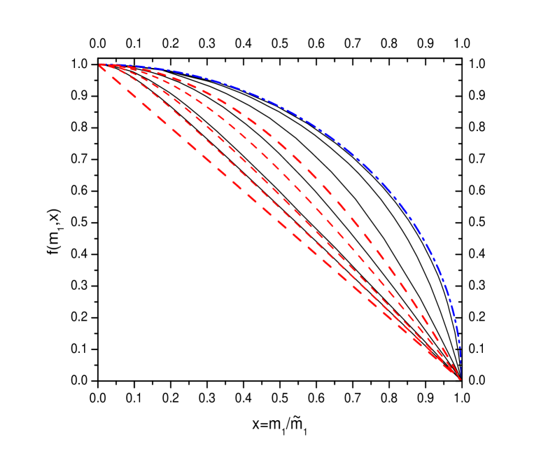
Figure 5: function $f$ calculated from the Eq.’s (49), (50) and (51) and plotted vs. $x\equiv m_{1}/\widetilde{m}_{1}$ for $m_{1}/m_{\rm atm}=5,2,1,0.5,0.2,0.1$ (from the top to the bottom solid line). The hierarchical limit for $f$ (cf. (56)) is plotted for $m_{1}/m_{\rm atm}=1,0.5,0.2,0.1,0.01$ (from the top to the bottom dashed line), while the quasi-degenerate limit (cf. Eq. (46)) corresponds to the dot-dashed line.

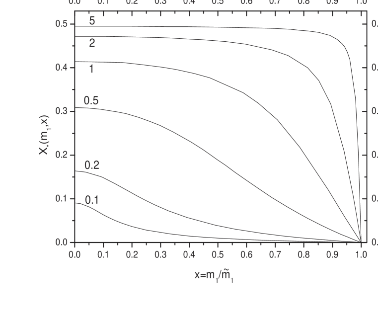
Figure 6: $X_{\star}$ calculated from the Eq.’s (49) and (50) as a function of $x\equiv m_{1}/\widetilde{m}_{1}$ and for the indicated values of $m_{1}/m_{\rm atm}$.

It is also possible to derive explicitly analytic expressions for the functions $X_{\star}$ and $Y_{\rm m}$. However these are algebraically quite involved and not useful to be written down, while the two equations (49) and (50) provide a much more useful physical insight and at the same time simple and useful explicit analytical expressions can be easily derived in some interesting limits:

• in the limit of fully hierarchical neutrinos one obtains $X_{\star}=0$ and $Y_{\rm m}=\widetilde{m}_{1}/m_{3}$, implying the already well known result $f(m_{1},\widetilde{m}_{1})=1$;

• in the limit of quasi-degenerate neutrinos, for $m_{1}\simeq m_{3}$, one gets from the Eq. (50) $X_{\star}=1/2$, that inserted in the Eq. (49) gives once more $f(m_{1},\widetilde{m}_{1})=\sqrt{1-(m_{1}/\widetilde{m}_{1})^{2}}$;

• in general, since $0\leq m_{1}/m_{3}\leq 1$, one has $0\leq X_{\star}\leq 1/2$;

• if $\widetilde{m}_{1}=m_{1}$ then $X=Y=f=0$ and vice versa;

• in the limit $\widetilde{m}_{1}\gg m_{1}$ one gets easily $Y_{\rm m}(m_{1},\widetilde{m}_{1}\gg m_{1})=\widetilde{m}_{1}/(m_{1}+m_{3})$, corresponding to the already known result $f(m_{1},\widetilde{m}_{1}\gg m_{1})=1$, and also $X_{\star}(m_{1},\widetilde{m}_{1}\gg m_{1})=m_{1}/(m_{1}+m_{3})$.

It is also easy to go beyond the limit of fully hierarchical neutrinos and find an expression for the function $f(m_{1},\widetilde{m}_{1})$ valid in the regime $m_{1}/m_{\rm atm}\lesssim 1$, corresponding to $m_{1}\lesssim m_{3}/\sqrt{2}$. The equation (50) can be conveniently re-casted in the following form

$${X_{\star}/Y_{\rm m}\over\sqrt{1+X_{\star}^{2}/Y_{\rm m}^{2}}}={m_{1}\over m_{3}}\,{(1-X_{\star})/Y_{\rm m}\over\sqrt{1+(1-X_{\star})^{2}/Y_{\rm m}^{2}}},$$ (52)

from which one can see that

$${X_{\star}\over Y_{\rm m}}\leq{m_{1}\over\sqrt{m_{3}^{2}-m_{1}^{2}}}\,$$ (53)

and from this it follows that $X_{\star}\leq m_{1}/(\sqrt{2}\,m_{3})$. Neglecting terms ${\cal O}(m_{1}^{2}/m_{3}^{2})$ one can then find the approximate relation

$$X_{\star}\simeq{m_{1}\over m_{3}}\,{Y_{\rm m}\over\sqrt{1+Y_{\rm m}^{2}}},$$ (54)

while the Eq. (49) becomes simply

$$m_{1}\,\sqrt{Y_{\rm m}^{2}+1}+m_{3}\,Y_{\rm m}=\widetilde{m}_{1}\,.$$ (55)

It is in the end easy to obtain the expression

$$f(m_{1},\widetilde{m}_{1})={m_{3}-m_{1}\,\sqrt{1+{m^{2}_{3}-m^{2}_{1}\over\widetilde{m}_{1}^{2}}}\over m_{3}-m_{1}},$$ (56)

valid at the first order in $m_{1}/m_{3}$, while at the zero-th order in $m_{1}/m_{3}$ and $\widetilde{m}_{1}/m_{3}$ (thus for $m_{\rm atm}\simeq m_{3}\gg\widetilde{m}_{1}\geq m_{1}$) it becomes simply $f(m_{1},\widetilde{m}_{1})=1-m_{1}/\widetilde{m}_{1}$. The expression (56) has been found in [10] assuming $X_{\star}=0$ and used to get an upper bound on the absolute neutrino mass scale $m_{i}\leq 0.1\,{\rm eV}$. This function clearly does not describe the function $f(m_{1},\widetilde{m}_{1})$ for any value of $m_{1}$. In Fig. 5 one can see (dashed lines) how for increasing values of $m_{1}/m_{\rm atm}$, from $0.01$ to $1$, the function saturates to its asymptotic limit $f=1-(m_{1}/\widetilde{m}_{1})^{2}$ and so, in particular, it does not reproduce the correct bound represented by the Eq. (46) [19]. However for values $m_{1}\simeq 2\,m_{\rm atm}\simeq 0.1\,{\rm eV}$, those corresponding to the bound on neutrino masses, it underestimates the bound on the $C\!P$ asymmetry at most of $\sim 20\%$ (see Fig. 5 and compare with the solid line for $m_{1}/m_{\rm atm}=2$) and the neutrino mass upper bound itself is therefore underestimated only of $\sim 5\%$ (corresponding to $\sim 0.01\,{\rm eV}$) [7], much below the precision of the bound itself. This, together with the result that we have just shown, for which this function is correct in the limit $(m_{1}/m_{3})^{2}<1$, fully justifies its approximate use for an arbitrary value of $m_{1}$ and is particularly interesting in connection with a search of the neutrino mass upper bound when some restriction on the space of relevant parameters is introduced, such that the neutrino mass bound becomes more stringent and thus it falls in the region $(m_{1}/m_{3})^{2}<1$. This is for example the case when a cut-off $M_{1}^{\star}\lesssim 10^{12}\,{\rm GeV}$ on the value of $M_{1}$ is imposed [10, 32]. In Section 6 we will also show another ueful application of the Eq. (56). We have also compared the exact $f(m_{1},\widetilde{m}_{1})$, given by the equations (49), (50) and (51) and plotted in Fig. 5 (solid lines), with the results obtained in [19] using the approximation $m_{\rm sol}=0$. We have found a slight difference, within a few per cent, for $m_{1}\simeq\widetilde{m}_{1}$, getting completely negligible as soon as $\widetilde{m}_{1}$ is appreciably larger than $m_{1}$.

5 The effective leptogenesis phase

In the previous section we have characterized which are the configurations that maximize the $C\!P$ asymmetry, or equivalently for which the effective phase $\sin\delta_{L}=1$. Here we want to study how easily this condition can be realized and which are the typical values of the phase for different classes of configurations. In general we can write, from its definition (cf. (33),(38),(42)),

$$\sin\delta_{L}(m_{1},\widetilde{m}_{1},\Omega_{j1}^{2})={m_{1}+m_{3}\over\widetilde{m}_{1}\,\,f(m_{1},\widetilde{m}_{1})}\,(Y_{3}+\sigma^{2}\,Y_{2}),$$ (57)

where $\sigma\equiv\sqrt{\Delta m^{2}_{21}}/m_{\rm atm}$ is given by $m_{\rm sol}/m_{\rm atm}$ or by $\sqrt{1-m_{\rm sol}^{2}/m_{\rm atm}^{2}}$, depending on whether the case of normal or inverted hierarchy is considered. The expression (57) can be also recasted as

$$\sin\delta_{L}(m_{1},\widetilde{m}_{1},\Omega_{j1}^{2})={m_{1}+m_{3}\over f(m_{1},\widetilde{m}_{1})}\,\left({\rho_{3}\sin\varphi_{3}+\sigma^{2}\,\rho_{2}\sin\varphi_{2}\over m_{1}\,\rho_{1}+m_{2}\,\rho_{2}+m_{3}\,\rho_{3}}\right)\,,$$ (58)

showing that the effective phase reduces to genuine phases in particular cases, while in general it is given by a linear combination of them, analogously to how the effective neutrino mass $\widetilde{m}_{1}$ is a linear combination of the neutrino masses, with coefficients given by the $\rho_{j}$’s in both cases. It should be stressed that, in the general framework we are considering, it does not depend on the phases that could be responsible for $C\!P$ violation at low energies and contained in the mixing matrix $U$. The requirement of successful leptogenesis implies the lower bound

$$\sin\delta_{L}(m_{1},\widetilde{m}_{1},\Omega_{j1}^{2})\geq{\eta_{B}^{CMB}\over\eta_{B}^{\rm max}(M_{1},m_{1},\widetilde{m}_{1})}\,,$$ (59)

that, together with the lower bounds on $M_{1}$ and on $T_{\rm reh}$, represents another useful way to get information on the $\Omega$-parameters through leptogenesis. For practical purposes it is interesting to study the effective phase in the two asymptotic limits of fully hierarchical neutrinos and quasi-degenerate neutrinos.

5.1 Fully hierarchical neutrinos

In this case one has $m_{1}=0$, $m_{3}=m_{\rm atm}$ and $f=1$ and the general expression (58) becomes

$$\sin\delta_{L}={m_{\rm atm}\over\widetilde{m}_{1}}\,\left[\rho_{3}\sin\varphi_{3}+\sigma^{2}\rho_{2}\sin\varphi_{2}\right]\,,$$ (60)

where now simply $\widetilde{m}_{1}=m_{2}\,\rho_{2}+m_{\rm atm}\,\rho_{3}$ and $m_{2}=m_{\rm sol}\,(\simeq m_{\rm atm})$ in the case of normal (inverted) hierarchy. The value of the phase in the full hierarchical case is relevant in connection with the ($3\,\sigma$) lower bound on $M_{1}$ given by

$$M_{1}\gtrsim{4.2\times 10^{8}\,{\rm GeV}\over\kappa_{\rm f}(\widetilde{m}_{1})\,\sin\delta_{L}}\hskip 28.45274pt(M_{1}\ll 10^{14}\,{\rm GeV})\,,$$ (61)

that generalizes the case of maximal phase considered in [8]. When thermal effects on the Higgs mass are taken into account and a proper subtraction procedure of on shell $\Delta L=2$ processes is employed [33], the efficiency factor can be approximately calculated accounting only for decays and inverse decays [7]. In any case this provides a conservative upper bound, since other effects, in particular those arising from spectator processes [34], can only lower the final asymmetry. Then a very good analytical approximation in the case of an initial thermal abundance, that gives quite a conservative upper limit in the weak wash-out regime, is

$$k_{\rm f}(\widetilde{m}_{1})\simeq{2\over K\,z_{B}(K)}\,\left(1-e^{-{K\,z_{B}(K)\over 2}}\right)\,,$$ (62)

where the decay parameter $K$ is related to the effective neutrino mass through the relation

$$K={\widetilde{m}_{1}\over m_{\star}}\simeq 926\,{\widetilde{m}_{1}\over{\rm eV}}\,,$$ (63)

while the baryogenesis $z\equiv M_{1}/T$ value is calculated using

$$z_{B}(K)\simeq 9/8+2.35\,[\ln(1+K)]^{0.8}\,.$$ (64)

A comparison between the analytical approximation (cf. (62) and (64)) and the numerical solution is shown in Fig. 7 while the lower bound on $M_{1}$ is plotted in Fig. 8.

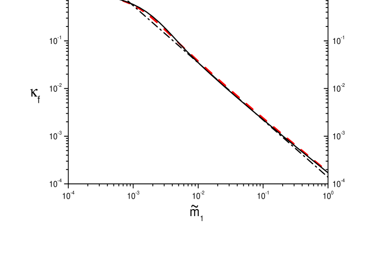
Figure 7: Efficiency factor: the analytic approximation (dashed line) given by the eq.’s (62) and (64) is compared with the numerical solution (solid line) of the kinetic equations when the wash-out from scatterings is neglected and an initial thermal $N_{1}$ abundance is assumed [7]. The dot-dashed line is the power-law fit eq. (65).

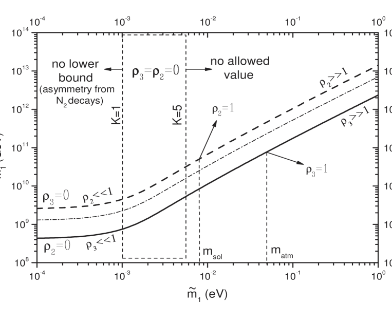
Figure 8: Lower bounds ($3\sigma$) on $M_{1}$ for different value of the effective phase in the case of normal hierarchy. The solid line corresponds to maximal phase in the case $\rho_{2}=0$ (cf. (61)). The dashed line corresponds to the case $\rho_{3}=0$ and is given by the Eq. (61) with $\sin\delta_{L}=\sigma\simeq 1/6$. The dot-dashed line is the intermediate case $\rho_{3}=\sigma^{2}\,\rho_{2}$ with an effective phase $\sin\delta_{L}=2\,\sigma\simeq 1/3$. The box indicates a transition range of $\widetilde{m}_{1}$ values in the scenario where the asymmetry is generated by the $N_{2}$’s decays for $\rho_{3}=\rho_{2}=0$: for $\widetilde{m}_{1}\lesssim m_{\star}\,(K\lesssim 1)$ there is no lower bound on $M_{1}$, while for $\widetilde{m}_{1}\gtrsim 5\,m_{\star}\,(K\gtrsim 5)$ there is no allowed value.

For $0.5\,m_{\rm sol}\lesssim\widetilde{m}_{1}\lesssim 2\,m_{\rm atm}$ the expression (62) can be approximated with the power law [32]

$$k_{\rm f}(\widetilde{m}_{1})\simeq{0.5\over K^{1.2}}\simeq 3.5\times 10^{-2}\,\left({10^{-2}\,{\rm eV}\over\widetilde{m}_{1}}\right)^{1.2}\,$$ (65)

and in the range $\widetilde{m}_{1}=[m_{\rm sol},m_{\rm atm}]$ one gets, from the Eq. (61), $M_{1}\gtrsim(10^{10}-10^{11})\,{\rm GeV}$. Notice that only for $K\gtrsim 5$ the lower bound on $M_{1}$ does not depend on the initial conditions and in particular on a specific description of $N_{1}$’s production. The lower bound at $K\simeq 5$, $M_{1}\gtrsim 5\times 10^{9}\,{\rm GeV}$, is thus particularly meaningful, since it can be regarded as the lowest allowed $M_{1}$ value without the need of additional assumptions beyond the given ones.

Within the minimal supersymmetric standard model (MSSM) the $C\!P$ asymmetry and its maximum value get double and this implies a relaxation of the lower bound Eq. (61) at low $\widetilde{m}_{1}$, such that [32]

$$M_{1}\gtrsim{2.25\times 10^{8}\,{\rm GeV}\over\kappa_{\rm f}(\widetilde{m}_{1})\,\sin\delta_{L}}\hskip 28.45274pt(M_{1}\ll 10^{14}\,{\rm GeV})\,.$$ (66)

The expression (62) for the efficiency factor is still valid but the stronger wash-out processes make the equilibrium neutrino mass a bit lower than in the SM case, $m_{\star}^{MSSM}\simeq 0.0008\,{\rm eV}$, such that $K\simeq 1270\,\widetilde{m}_{1}/{\rm eV}$. In this way the efficiency factor in the strong wash out regime gets also lower and the power law (65) becomes [32]

$$k_{\rm f}\simeq{0.5\over{K}^{1.2}}\simeq 2.4\times 10^{-2}\,\left({10^{-2}\,{\rm eV}\over\widetilde{m}_{1}}\right)^{1.2}\,,$$ (67)

while the $3\sigma$ lower bound on $M_{1}$ in the range $\widetilde{m}_{1}=[m_{\rm sol},m_{\rm atm}]$ becomes just slightly more relaxed. Within a thermal picture of leptogenesis, as we are assuming, the lower bound on $M_{1}$ is closely related to a lower bound on the reheating temperature of the early Universe $T_{\rm reh}$ that is approximately given by the expression [7]

$$T_{\rm reh}^{\rm min}\simeq{M_{1}^{\rm min}\over z_{B}-2\,e^{-\alpha/K}}\,,$$ (68)

plotted in Fig. 9 for $\alpha=0.5$ .

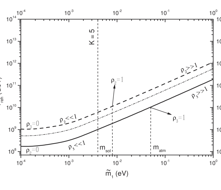
Figure 9: Lower bound ($3\,\sigma$) on $T_{\rm reh}$ in the MSSM case (cf. (68)). The lines correspond to the same cases of fig 7. For values $K\gtrsim 5$ (right of the dashed line) the lower bound does not depend on the initial conditions.

For $K\simeq 5$ one has the lowest $T_{\rm reh}$ value independent on the choice of initial conditions and conservatively we obtain $T_{\rm reh}\gtrsim 10^{9}\,{\rm GeV}$.

The existence of such a lower bound on $T_{\rm reh}$ represents a problem within the MSSM picture, since this has to be compared with the upper bound from the avoidance of the gravitino problem. Values of the gravitino mass $\ll 100\,{\rm TeV}$ require reheating temperature $T_{\rm reh}\ll 10^{10}\,{\rm GeV}$ [35]. From Fig. 9 one can see that there is compatibility only for values $\widetilde{m}_{1}\ll m_{\rm atm}$.

These results are valid under the conservative assumption of maximal phase. In general, if one modifies the picture such that the final predicted asymmetry $\eta_{B}\rightarrow\xi\,\eta_{B}$, then the lower bound on $M_{1}$ and on the reheating temperature change as $(M_{1}^{\rm min},T_{\rm reh}^{\rm min})\rightarrow(M_{1}^{\rm min},T_{\rm reh}^{\rm min})/\xi$ [9]. Therefore, if we consider models with some phase suppression, $\sin\delta_{L}<1$, the minimum allowed values of $M_{1}$ and $T_{\rm reh}$ increase compared to the case of maximal phase. On the other hand, if $M_{1}^{\rm min}$ becomes larger than about $10^{14}\,{\rm GeV}$, the assumption that $\kappa_{\rm f}$ depends only on $\widetilde{m}_{1}$ is not valid any more, since $\Delta L=2$ processes give an additional contribution to the wash-out depending also on $M_{1}$ [8]. In this case the efficiency factor is exponentially suppressed at large $M_{1}$ values such that

$$\kappa_{\rm f}(\widetilde{m}_{1})\rightarrow\kappa_{\rm f}(\widetilde{m}_{1})\,e^{-{\omega\over z_{B}}\,{M_{1}\over 10^{14}\,{\rm GeV}}}\,,\hskip 28.45274pt(\omega\simeq 5)$$ (69)

and $\eta_{B}^{\rm max}(M_{1},m_{1}=0,\widetilde{m}_{1})$ (cf. (34)) has a maximum at $M_{1}\simeq 2\,z_{B}\,10^{13}\,{\rm GeV}$ given by [31]

$$\eta_{B}^{\rm max}(m_{1}=0,\widetilde{m}_{1})\simeq 1.5\times 10^{-5}\,{10^{-3}\,{\rm eV}\over\widetilde{m}_{1}}\,\,\;\;\;\,\,\,\,\,(\widetilde{m}_{1}\gtrsim 10^{-3}\,{\rm eV})\,.$$ (70)

This implies that the lower bound on the phase (cf. (59)) cannot be arbitrarily evaded increasing $M_{1}$ and one can place an interesting lower bound, independent on the value of $M_{1}$, given by

$$\sin\delta_{L}\geq\,4\times 10^{-5}\,{\widetilde{m}_{1}\over 10^{-3}\,{\rm eV}}\,\hskip 28.45274pt\,(\widetilde{m}_{1}\gtrsim 10^{-3}\,{\rm eV})\,.$$ (71)

Let us study two special cases. For $\rho_{2}=0$ one has $\widetilde{m}_{1}=\rho_{3}\,m_{\rm atm}$ and from the Eq. (60)

$$\sin\delta_{L}=\sin\varphi_{3}\,.$$ (72)

One can set $\delta_{L}=\varphi_{3}$, fixing unambiguously $\delta_{L}$. Again one can see that the effective leptogenesis phase is maximal for $\rho_{2}=0$ (i.e. $\Omega_{21}=0$) and $X_{3}=0$, corresponding to $\varphi_{3}=\pi/2$. For random assignations of $\varphi_{3}$, the average value of the phase, $\langle|\sin\varphi_{3}|\rangle=2/\pi\simeq 0.6$, suggests that a value close to the maximal one is a reasonable possibility not requiring any particular tuning.

Within models with single or sequential RH neutrino dominance, characterized by $|X_{j}|\simeq 1\gg|X_{i\neq j}|$, there are two choices: either $X_{1}\simeq 1\gg|X_{3}|$ or conversely $X_{3}\simeq 1\gg|X_{1}|$. The first one corresponds to maximal phase $\sin\delta_{L}\simeq 1$, while $\widetilde{m}_{1}\simeq Y_{3}\,m_{\rm atm}$. If furthermore one has $Y_{3}\ll 1$, then one has the kind of models we previously discussed, with $\Omega$ obtained as a small complex perturbation of the matrix (25) and small values of $\widetilde{m}_{1}\ll m_{\rm atm}$, such that minimum values $M_{1},T_{\rm reh}\sim 10^{9}\,{\rm GeV}$ are possible. In the second case, i.e. $X_{3}\simeq 1\gg|X_{1}|$, such that $N_{1}$ contributes only to $m_{3}$, one has necessarily some phase suppression and moreover $\widetilde{m}_{1}\geq m_{\rm atm}$. The value of the phase can be expressed as a function of $\widetilde{m}_{1}$ and is given by $\sin\delta_{L}=\sqrt{1-{m_{\rm atm}^{2}/\widetilde{m}_{1}^{2}}}$. Since the efficiency factor is approximately inversely proportional to $\widetilde{m}_{1}$ (cf. (65)), then one easily finds that the final asymmetry $\eta_{B}(m_{1}=0,\widetilde{m}_{1})\propto\kappa_{\rm f}(\widetilde{m}_{1})\,\sin\delta_{L}(\widetilde{m}_{1})$ is maximized for $\widetilde{m}_{1}\simeq\sqrt{2}\,m_{\rm atm}$ corresponding to $\sin\delta_{L}\simeq 1/\sqrt{2}$. This implies a much more stringent lower bounds on $M_{1}$ and on $T_{\rm reh}$ that can be read from Fig.’s 8 and 9 obtaining $M_{1}\gtrsim 1.5\times 10^{11}\,{\rm GeV}$ and $T_{\rm reh}\gtrsim 2\times 10^{10}\,{\rm GeV}$. Moreover the lower bound on the phase (cf. (71)) becomes $\sin\phi_{3}\gtrsim 2\times 10^{-3}$.

Still another possibility is that $N_{1}$ contributes both to $m_{1}$ and to $m_{3}$ and in this case $|X_{1}|\sim|X_{3}|\gtrsim 1$, such that $\widetilde{m}_{1}\gtrsim m_{\rm atm}$, still implying $M_{1}\gtrsim 10^{11}\,{\rm GeV}$ and $T_{\rm reh}\gtrsim 10^{10}\,{\rm GeV}$.

The second special case is for $\rho_{3}=0$, such that $\widetilde{m}_{1}=m_{2}\,\rho_{2}$ and from the Eq. (60) one obtains

$$\sin\delta_{L}=\sigma\sin\varphi_{2}\,.$$ (73)

If one considers the case of normal hierarchy, then $\sigma=m_{\rm sol}/m_{\rm atm}\simeq 1/6$ and this unavoidably leads to a strong phase suppression, $\sin\delta_{L}\simeq\sin\varphi_{2}/6\ll 1$, that results in a more stringent bound on $M_{1}$ (see the dashed line in Fig. 8) and on $T_{\rm reh}$ (see the dashed line in Fig. 9). For models with $N_{1}$ contributing only to $m_{2}$, such that $X_{2}\simeq 1\gg|X_{1}|$, the phase suppression is $\sin\delta_{L}<1/6$, and similar lower bounds for $M_{1}$ and $T_{\rm reh}$, as in the case of $N_{1}$ contributing only to $m_{3}$, hold, even though the wash-out is much weaker because now $\widetilde{m}_{1}\simeq m_{\rm sol}\ll m_{\rm atm}$.

We have thus two extreme cases, $\rho_{2}=0$ or $\rho_{3}=0$, where the effective phase can be maximal or remarkably suppressed. Let us now analyze the general case, with both non-vanishing $\rho_{2}$ and $\rho_{3}$. Since we are interested in the lower bound on $M_{1}$, we can study the expression (60) for maximal phases, $\sin\varphi_{2}=\sin\varphi_{3}=1$, and thus

$$\sin\delta_{L}={\rho_{3}+\sigma^{2}\rho_{2}\over\rho_{3}+\sigma\rho_{2}}\,.$$ (74)

These are the most general models with $N_{1}$ contributing only to $m_{1}$, such that $|X_{2}|,|X_{3}|\ll X_{1}\simeq 1$. For $\rho_{3}\gg\sigma\rho_{2}$ one has $\sin\delta_{L}\simeq 1$ and $\widetilde{m}_{1}\simeq\rho_{3}\,m_{\rm atm}$, such that the limit $\rho_{2}=0$ is recovered, while conversely, for $\rho_{3}\ll\sigma^{2}\,\rho_{2}$, one has the phase suppression $\sin\delta_{L}=\sigma\simeq 1/6$ and $\widetilde{m}_{1}\simeq\rho_{2}\,m_{\rm sol}$ and one recovers the limit $\rho_{3}=0$.

In the intermediate case, $\sigma^{2}\rho_{2}\lesssim\rho_{3}\lesssim\sigma\rho_{2}$, one has $2\,\sigma\lesssim\sin\delta_{L}\lesssim 1/2$. For example for $\rho_{3}=\sigma\rho_{2}$ one has $\widetilde{m}_{1}=2\,m_{\rm sol}\simeq 0.016\,{\rm eV}$ and $\sin\delta_{L}=1/2$ corresponding to $M_{1}\gtrsim 4\times 10^{10}\,{\rm GeV}$ and $T_{\rm reh}\gtrsim 7\times 10^{9}\,{\rm GeV}$. For $\rho_{3}=\sigma^{2}\,\rho_{2}\ll 1$ one has $\sin\delta_{L}=2\,\sigma\simeq 1/3$ and $\widetilde{m}_{1}\simeq m_{\rm sol}\,\rho_{2}$. The corresponding lower bounds on $M_{1}$ and $T_{\rm reh}$ are shown in Fig. 8 and 9 (dot-dashed lines). If $\rho_{2}=1$ one gets $M_{1}\gtrsim 3\times 10^{10}\,{\rm GeV}$ and $T_{\rm reh}\gtrsim 5\times 10^{9}\,{\rm GeV}$. Therefore, this case represents the best compromise to get the lowest possible values for $T_{\rm reh}$ and $M_{1}$ without having $\rho_{2},\rho_{3}\ll 1$ and $\rho_{1}\simeq 1$.

We can conclude that the possibility to access the window $10^{9}\lesssim M_{1}\,(T_{\rm reh})/{\rm GeV}\lesssim(0.5)\,3\,\times\,10^{10}$ relies on a particular class of models, such that $\rho_{2},\rho_{3}\ll\rho_{1}\simeq 1$, the only ones allowing both maximal phase and $\widetilde{m}_{1}\ll m_{\rm atm}$. This conclusion does not change if one considers the case of inverted hierarchy: it is true that one does not have phase suppression but values of $\widetilde{m}_{1}\ll 10^{-2}\,{\rm eV}$ are obtained again only for $\rho_{2},\rho_{3}\ll 1\simeq\rho_{1}$.

More generally values $T_{\rm reh}\lesssim 10^{10}\,{\rm GeV}$ are obtained only within models where $N_{1}$ contributes only to $m_{1}$. Among sequential dominated models these correspond to models where $m_{1}$ is dominantly determined just by $N_{1}$. For models where $N_{1}$ contributes only to $m_{3}$, including sequential dominated models with $m_{3}$ dominated by $N_{1}$, we have seen that, if $\rho_{2}=0$, then necessarily the lower bounds are more restrictive, such that $M_{1}\gtrsim 1.5\times 10^{11}\,{\rm GeV}$ and $T_{\rm reh}\gtrsim 2\times 10^{10}\,{\rm GeV}$. Allowing a non zero $Y_{2}$ the bounds can only become more restrictive. On the other hand if one considers models where $N_{1}$ contributes dominantly only to $m_{2}$ ($X_{2}\simeq 1\gg X_{1},X_{3}$), including those where $m_{2}$ is dominated by $N_{1}$, the limits obtained for $\rho_{3}=0$ can be relaxed if one allows a non zero $Y_{3}$. The best optimization between high phase and low $\widetilde{m}_{1}$ is obtained for configurations with $Y_{2}=0$. In this case one has $\sin\delta_{L}=1-m_{\rm sol}/\widetilde{m}_{1}$ and it is simply to see that the asymmetry is maximized for $\widetilde{m}_{1}\simeq 2\,m_{\rm sol}$ corresponding to $\sin\delta_{L}\simeq 0.5$. One then obtains $M_{1}\gtrsim 4\times 10^{10}\,{\rm GeV}$ (within SM) and $T_{\rm reh}\gtrsim 7\times 10^{9}\,{\rm GeV}$ (within MSSM) .

5.2 Quasi-degenerate neutrinos

In this case one has $m_{1}\simeq m_{2}\simeq m_{3}$ and thus $m_{1}/\widetilde{m}_{1}\simeq{\ell}^{-1}$, where remember that ${\ell}\equiv\rho_{1}+\rho_{2}+\rho_{3}\geq 1$. The expression (46) can then be re-casted as $f\simeq\sqrt{{\ell}^{2}-1}/{\ell}$ and the Eq. (58) for the phase becomes

$$\sin\delta_{L}\simeq{2\over\sqrt{\ell^{2}-1}}\,[\rho_{3}\sin\varphi_{3}+\sigma^{2}\rho_{2}\sin\varphi_{2}]\,.$$ (76)

For $\rho_{2}=0$ and $X_{3}=1/2$ one has $Y_{3}=2/\sqrt{\ell^{2}-1}$ and the case of maximal phase is recovered. On the other hand if one considers models with $\rho_{3}=0$, then the maximum asymmetry is still realized for $X_{2}=1/2$ but this time one has $\sin\delta_{L}=\sigma^{2}$, meaning that if $\sigma=m_{\rm atm}/m_{\rm sol}\simeq 1/6$ (‘normal’ quasi-degenerate spectrum), then one has a strong phase suppression, $\sigma$ times stronger than in the case of fully hierarchical neutrinos.

We can also consider an intermediate case with both $\rho_{2}$ and $\rho_{3}\neq 0$, for example when $\varphi_{2}=\varphi_{3}$ and $X=1/2$ (dot-dashed arrows in Fig. 10).

Figure 10: quasi-degenerate neutrinos; three different cases with non maximal phase, as considered in the main text.

In this case the general expression (76) gets specialized into $\sin\delta_{L}=1-\zeta+\sigma^{2}\,\zeta$, where $\zeta=\rho_{2}/(\rho_{2}+\rho_{3})$, and describes the transition between the case with $\rho_{2}=0$ and the case with $\rho_{3}=0$.

Another example is given by a situation where $\rho_{2}=0$ but the condition $X_{3}=1/2$ is not realized. For example if one takes $X_{3}=0$ (see solid arrows in Fig. 10), then one gets $\sin\delta_{L}=\sqrt{1-1/{\ell}^{2}}$. For ${\ell}\gg 1$, corresponding to $\widetilde{m}_{1}\gg m_{1}$, one recovers maximal phase, while for finite values of $\widetilde{m}_{1}$ there is some phase suppression. An interesting example is to take $\widetilde{m}_{1}=\sqrt{2}\,m_{1}$, since this corresponds to the peak value that saturates the upper bound on neutrino masses [7]. In this particular case one finds $\sin\delta_{L}=\sqrt{1/2}\simeq 0.7$. An analogous result holds if one takes $X_{1}=0$ and $X_{3}=1$. Notice that these two cases correspond to a lightest neutrino mass dominated by the lightest RH neutrino (for $X_{3}=0$) or by the heaviest (for $X_{1}=0$).

We have also considered the case of configurations with $Y_{2}=0$ and $X_{3}=(1-X_{2})/2$, such that when $X_{2}=0$ one recovers the configuration with maximal phase (dashed arrows in Fig. 10). In this case one obtains easily

$$\sin\delta_{L}=\sqrt{1-{2\,X_{2}\over\ell+1}}\,$$ (77)

and for example, for $\rho_{2}={\ell}/3$, one gets $\sin\delta_{L}\simeq 0.7$. These examples show that typically a phase suppression is expected. This is relevant in connection with the neutrino mass upper bound, $m_{i}\leq 0.1\,{\rm eV}$, because it implies that the saturation of the bound actually occurs, not only for special values of $M_{1}$ and $\widetilde{m}_{1}$, but also for special $\Omega_{j1}$’s configurations.

6 A new scenario of thermal leptogenesis

So far we have assumed that the final asymmetry is not influenced by the two heavier RH neutrinos and this has considerably reduced the number of seesaw parameters on which the final asymmetry depends. This assumption holds if the asymmetry generated by the $N_{2}$’s and by the $N_{3}$’s is either negligible or is efficiently washed-out by the inverse decays of the $N_{1}$’s and also if the approximated expression (30) for the $C\!P$ asymmetry $\varepsilon_{1}$ can be used. As we will discuss in Section 7, these two conditions require some degree of hierarchy in the heavy neutrino spectrum. Here, even though we still assume a hierarchical heavy neutrino spectrum, we study a scenario where the final asymmetry is produced by the $N_{2}$’s decays. This is possible if the value of the effective neutrino mass lies in the weak wash-out regime. In this case the wash-out from $N_{1}$ inverse decays and scatterings is not sufficient to wash-out a previously generated asymmetry, in particular that one generated from the $N_{2}$’s decays. As we discussed in Section 2, the possibility that $\widetilde{m}_{1}\lesssim m_{\star}\simeq 10^{-3}\,{\rm eV}$, relies on models with an $\Omega$ matrix obtained as a small perturbation of a 23-rotation in the complex plane (cf.(25)). Naively one could think that, since we are still assuming a hierarchical spectrum of neutrinos such that $M_{2}\gg M_{1}$, and because of the lower bound on $M_{1}$, one has to require large values of the reheating temperature such that $T_{\rm reh}\gtrsim M_{2}\gg 10^{9}\,{\rm GeV}$. However, it is easy to understand that actually the lower bound on $M_{1}$ disappears and is simply replaced by an analogous lower bound on $M_{2}$. First of all let us notice that in a general case the final asymmetry is the sum of the contributions from all the three $N_{i}$’s and, assuming a sufficiently hierarchical heavy neutrino spectrum, it can be written as

$$\eta_{B}={a_{\rm sph}\over N_{\gamma}^{\rm rec}}\;\sum_{i}\,\varepsilon_{i}\;\kappa_{\rm f,i}\,,$$ (78)

that generalizes the expression (17) with $\kappa_{\rm f,1}\equiv\kappa_{\rm f}$. Let us focus on the asymmetry produced by the $N_{2}$ decays. These will be described by a quantity, $\widetilde{m}_{2}$, that plays an analogous role of $\widetilde{m}_{1}$ in the description of the $N_{1}$ decays and is defined as

$$\widetilde{m}_{2}\equiv{\left(m^{\dagger}_{D}\,m_{D}\right)_{22}\over M_{2}}=\sum_{i}\,m_{i}\,\rho_{i2}\,.$$ (79)

For our purposes the $\Omega$ matrix can be conveniently parameterized in the following way

$$\Omega=\left(\begin{array}[]{ccc}\sqrt{1-\Omega_{21}^{2}-\Omega_{31}^{2}}&\Omega_{12}&-\sqrt{\Omega_{21}^{2}+\Omega_{31}^{2}-\Omega^{2}_{12}}\\ \Omega_{21}&\Omega_{22}&-\sqrt{1-\Omega_{22}^{2}-\Omega_{21}^{2}}\\ \Omega_{31}&\sqrt{1-\Omega_{22}^{2}-\Omega_{12}^{2}}&\sqrt{\Omega_{22}^{2}+\Omega^{2}_{12}-\Omega_{31}^{2})}\end{array}\right)\,.$$ (80)

The orthogonality also implies that each product of different columns or rows has to vanish. Therefore, we can still express one of the four left complex elements as a function of the other three. For example, if $\Omega_{21}\neq 1$, one can write

$$\Omega_{12}={-\Omega_{21}\,\Omega_{22}\,\sqrt{1-\Omega_{21}^{2}-\Omega_{31}^{2}}\pm\Omega_{31}\sqrt{1-\Omega_{21}^{2}-\Omega_{22}^{2}}\,\over 1-\Omega_{21}^{2}}\,.$$ (83)

Since we are assuming $\rho_{1}\simeq 1$ and $\rho_{2},\rho_{3}\ll 1$, this expression simplifies into

$$\Omega_{12}\simeq-\Omega_{21}\,\Omega_{22}\pm\Omega_{31}\,\sqrt{1-\Omega_{22}^{2}}\,,$$ (84)

from which one can deduce that $\rho_{12}\leq(\rho_{21}+\rho_{31})\,(1+\rho_{22})$, implying that it is impossible to have $\rho_{12}\simeq 1$ and $\rho_{22}\ll 1$. Therefore, if $\widetilde{m}_{1}\ll m_{\star}$, from the orthogonality of $\Omega$ it follows that is impossible to have $\widetilde{m}_{2}\ll m_{\star}$ too. This means that if the asymmetry from the $N_{1}$’s is generated in the weak wash-out regime, then the asymmetry from the $N_{2}$’s has necessarily to be generated in the strong wash-out regime. This is an interesting result because, if the final asymmetry is generated by the $N_{2}$’s, then it will be independent on the initial conditions exactly like in the typical case when the final asymmetry is generated by the $N_{1}$’s and $\widetilde{m}_{1}$ lies in the strong wash-out regime .

Moreover notice that a possible asymmetry generated by the heaviest RH neutrinos, the $N_{3}$’s, is always washed-out and negligible within the assumption of a hierarchical RH neutrino spectrum.

We have now to calculate the final asymmetry generated by the $N_{2}$’s and see whether this can explain the observed baryon asymmetry. Therefore, we have to calculate the $C\!P$ asymmetry associated to the $N_{2}$ decays. The expression for $\varepsilon_{2}$ is simply given by an expression similar to the Eq. (26),

$$\varepsilon_{2}\simeq-{1\over 8\pi}\sum_{i=1,3}\,{{\rm Im}\,\left[(h^{\dagger}\,h)^{2}_{2i}\right]\over(h^{\dagger}\,h)_{22}}\,\times\,\left[f_{V}\left({M^{2}_{i}\over M^{2}_{2}}\right)+f_{S}\left({M^{2}_{i}\over M^{2}_{2}}\right)\right]\,.$$ (85)

This time however it cannot be written in the form (30), since now the two terms have to be evaluated in two different limits: the first one ($i=1$) for $M_{1}^{2}/M_{2}^{2}\ll 1$ such that

$$f_{V}\left({M_{1}^{2}\over M_{2}^{2}}\right)+f_{S}\left({M_{1}^{2}\over M_{2}^{2}}\right)\simeq-\,{M_{1}\over M_{2}}\,\left(\ln{M_{2}\over M_{1}}-2\right)$$ (86)

and the second one ($i=3$) in the limit $M_{3}^{2}/M_{2}^{2}\gg 1$ such that

$$f_{V}\left({M_{3}^{2}\over M_{2}^{2}}\right)+f_{S}\left({M_{3}^{2}\over M_{2}^{2}}\right)\simeq-{3\over 2}\,{M_{2}\over M_{3}}\,.$$ (87)

In these limits the Eq. (85) becomes

$$\varepsilon_{2}\simeq{1\over 8\pi\,(h^{\dagger}\,h)_{22}}\left[{3\,M_{2}\over 2\,M_{3}}\,{\rm Im}[(h^{\dagger}h)^{2}_{23}]+{M_{1}\over M_{2}}\,\left(\ln{M_{2}\over M_{1}}-2\right)\,{\rm Im}[(h^{\dagger}\,h)_{21}^{2}]\right]\,.$$ (88)

From the Eq. (5) one can easily derive the relation

$$(h^{\dagger}\,h)_{ij}={\sqrt{M_{i}\,M_{j}}\over v^{2}}\sum_{h}\,\,m_{h}\,\Omega_{hi}^{\star}\,\Omega_{hj}\,,$$ (89)

that can be used to recast the Eq. (88) in terms of the $\Omega$ matrix elements and of $\widetilde{m}_{2}$ as

$$\varepsilon_{2}\simeq{3\,M_{2}\over 16\,\pi\,\widetilde{m}_{2}\,v^{2}}\left\{{\rm Im}\left[\sum_{h}\,m_{h}\,\Omega_{h2}^{\star}\,\Omega_{h3}\right]^{2}+{2\over 3}\,{M_{1}^{2}\over M_{2}^{2}}\,\left(\ln{M_{2}\over M_{1}}-2\right)\,{\rm Im}\,\left[\sum_{h}\,m_{h}\,\Omega_{h2}^{\star}\,\Omega_{h1}\right]^{2}\right\}\,.$$ (90)

Let us now consider three different limit cases of models where $\rho_{1}\simeq 1$ and $\rho_{2},\rho_{3}\ll 1$. The first case is for $\rho_{2}=0$ and $\rho_{22}=1$, corresponding to a small complex angle 13-rotation

$$\Omega=\left(\begin{array}[]{ccc}\sqrt{1-\Omega^{2}_{31}}&0&-\Omega_{31}\\ 0&1&0\\ \Omega_{31}&0&\sqrt{1-\Omega^{2}_{31}}\end{array}\right)\,.$$ (91)

As we know, in this case the $C\!P$ asymmetry $\varepsilon_{1}$ is maximal. On the other hand it is simple to see from the Eq. (90) that $\varepsilon_{2}=0$ and thus the asymmetry from the $N_{2}$’s vanishes and the traditional picture still holds. The second case is for $\rho_{3}=0$ and $\rho_{22}\simeq 1$, corresponding to a small complex angle 12-rotation

$$\Omega=\left(\begin{array}[]{ccc}\sqrt{1-\Omega^{2}_{21}}&-\Omega_{21}&0\\ \Omega_{21}&\sqrt{1-\Omega^{2}_{21}}&0\\ 0&0&1\end{array}\right)\,.$$ (92)

From the Eq. (90) one can easily see that the first term vanishes and one has

$$\varepsilon_{2}\simeq{M_{1}\,m_{\rm atm}\over 8\,\pi\,v^{2}}\,\sigma\,{M_{1}\over M_{2}}\,\left(\ln{M_{2}\over M_{1}}-2\right)\,\sin\varphi_{2}={2\over 3}\,\varepsilon_{\rm max}(M_{1})\,\sigma\,{M_{1}\over M_{2}}\,\left(\ln{M_{2}\over M_{1}}-2\right)\,\sin\varphi_{2}\,.$$ (93)

This result has to be compared with $\varepsilon_{1}=\varepsilon_{\rm max}(M_{1})\,\sigma\,\sin\varphi_{2}$ (cf. (31), (32) and (60)) showing that $\varepsilon_{2}\ll\varepsilon_{1}$. Therefore, in this second case too, one has that the asymmetry generated from the $N_{2}$’s can be neglected and again the usual picture still holds.

The most interesting case is for $\rho_{2}=\rho_{3}=0$, corresponding to a complex 23-rotation

$$\Omega=\left(\begin{array}[]{ccc}1&0&0\\ 0&\Omega_{22}&\sqrt{1-\Omega^{2}_{22}}\\ 0&-\sqrt{1-\Omega^{2}_{22}}&\Omega_{22}\end{array}\right)\,.$$ (94)

The second term in the Eq. (90) vanishes while the first, after some algebraic manipulations , gives

$$\varepsilon_{2}\simeq{3\,M_{2}\over 16\,\pi}\,{m^{2}_{3}-m^{2}_{2}\over v^{2}}\,{{\rm Im}(\Omega_{22}^{2})\over\widetilde{m}_{2}}\,,$$ (95)

showing that now $\varepsilon_{2}$ can be large, while on the other hand, as we know, $\varepsilon_{1}=0$. Therefore we see that, when $\widetilde{m}_{1}\ll m_{\star}$, the two possibilities of having maximum $C\!P$ asymmetry for the $N_{1}$ decays or for the $N_{2}$ decays are complementary and when one is maximum the other vanishes and vice versa.

The maximum value of $|\varepsilon_{2}|$ in the Eq. (95) can be found analogously to when we maximized $\varepsilon_{1}$ for configurations with $\Omega_{21}=0$. Now the role of $\Omega^{2}_{31}$ and $\Omega^{2}_{11}$ is replaced by $\Omega^{2}_{22}$ and $\Omega^{2}_{32}$ and one has to find the maximum of $Y_{22}\equiv{\rm Im}(\Omega_{22}^{2})$. This can be calculated solving a set of two algebraic equations for $Y_{22}^{\rm m}$ and for the corresponding value $X_{22}\equiv{\rm Re}(\Omega_{22}^{2})$, exactly equal to the Eq.’s (49) and (50) but with the obvious replacements $m_{1}\rightarrow m_{2}$ and $\widetilde{m}_{1}\rightarrow\widetilde{m}_{2}$. We can also introduce again a function $f(m_{2},\widetilde{m}_{2})$ related to $Y_{22}^{\rm m}$ exactly as the function $f(m_{1},\widetilde{m}_{1})$ was related to $Y_{\rm m}$ (cf. 51), writing

$$f(m_{2},\widetilde{m}_{2})={m_{2}+m_{3}\over\widetilde{m}_{2}}\,Y_{22}^{\rm m}\leq 1\,$$ (96)

and in this way one can write for the maximum $C\!P$ asymmetry

$$\varepsilon_{2}^{\rm max}=\varepsilon_{\rm max}(M_{2})\,{m_{3}-m_{2}\over m_{\rm atm}}\,f(m_{2},\widetilde{m}_{2})\,.$$ (97)

Notice that this is just the bound (43) for $\varepsilon_{1}$, where now $m_{1}$ is replaced by $m_{2}$ that is fixed, except for the possibility to choose between normal and inverted hierarchy. Therefore, this time $\varepsilon_{2}^{\rm max}$ depends on whether one considers normal or inverted hierarchy. The maximum value is obtained for normal hierarchy because in this case $m_{2}\ll m_{3}$ and also because the function $f(m_{2},\widetilde{m}_{2})$ cuts off the asymmetry for $\widetilde{m}_{2}\leq m_{2}$, that means for $\widetilde{m}_{2}\leq m_{\rm sol}$ in the normal case and for $\widetilde{m}_{2}\lesssim m_{\rm atm}$ in the inverted case. One can understand this difference also considering that in the case of inverted hierarchy one has a degeneracy $m_{2}\simeq m_{3}$ and thus it is analogous to the case of a quasi-degenerate spectrum for $\varepsilon_{1}$.

The bound (97) on $\varepsilon_{2}$ will give rise to a lower bound on $M_{2}$ analogously as the bound on $\varepsilon_{1}$ determined a lower bound on $M_{1}$ (cf. (61)). The difference is that now the function $f(m_{2},\widetilde{m}_{2})$ is less than one, even though we are dealing with hierarchical neutrinos and thus one has for the SM (MSSM) case

$$M_{2}\gtrsim{4.2\,(2.25)\times 10^{8}\,{\rm GeV}\over f(m_{2},\widetilde{m}_{2})\,\kappa_{\rm f}(\widetilde{m}_{2})}\,\,.$$ (98)

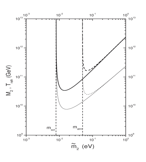
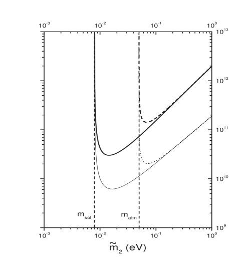
Figure 11: lower bounds ($3\,\sigma$) on $M_{2}$ (solid lines) and on $T_{\rm reh}$ (thin lines) obtained within models with $\widetilde{m}_{1}\ll m_{\star}$ and $\rho_{2}=\rho_{3}=0$. The solid lines refer to the case of normal hierarchy while the dashed lines refer to the case of inverted hierarchy. (left) SM case; (right) MSSM case.

This lower bound on $M_{2}$ is shown in Fig. 12 for both normal (thick solid line) and inverted (thick dashed line) hierarchy. Obviously, there will be again an associated lower bound on the reheating temperature given by the Eq. (68), where now $M_{1}^{\rm min}$ has to be replaced by $M_{2}^{\rm min}$. This lower bound on $T_{\rm reh}$ is also shown in Fig. 11 (thin lines). The lower bounds on $M_{2}$ and on $T_{\rm reh}$ can be calculated again both within the SM (Fig. 11 left) and the MSSM framework (Fig. 11 right).

Notice that within this scenario, with $\rho_{2}=\rho_{3}=0$, there is no lower bound on the value of $M_{1}$, that thus can be arbitrarily small. This occurs because we are assuming $\widetilde{m}_{1}\lesssim m_{\star}$, while if $\widetilde{m}_{1}\gtrsim 5\,m_{\star}$ the asymmetry from the $N_{2}$’s would be fully washed-out from the $N_{1}$ inverse decays and in this case there would not be any allowed value for $M_{1}$. Therefore, for $\rho_{2}=\rho_{3}=0$, there is a transition between a regime where the lower bound vanishes, for $\widetilde{m}_{1}/m_{\star}\ll 1$, and a regime where the lower bound goes to infinite, for $\widetilde{m}_{1}\gtrsim 5\,m_{\star}$. In the region $m_{\star}\lesssim\widetilde{m}_{1}\lesssim 5\,m_{\star}$ there is quite a sharp transition that can be determined by a detailed description of the wash-out of the asymmetry produced by the $N_{2}$’s from $N_{1}$ inverse decays. We have not calculated the lower bound in this transition region, that in Fig. 8 is schematically indicated with a box.

Since we are assuming $\rho_{3},\rho_{2}\ll\rho_{1}\simeq 1$, then approximately $m_{1}\simeq{v^{2}\,|\widetilde{h}_{11}|^{2}/M_{1}}$. Therefore, if $M_{1}$ becomes as low as the electroweak scale and because $m_{1}\ll 10^{-3}\,{\rm eV}$, then one has $|\widetilde{h}_{\rm 11}|\ll 10^{-7}$. This corresponds to a situation where the lightest right handed neutrino is decoupled and its interactions are switched-off, with no possibility to detect it in the accelerators .

Notice that one could also introduce an effective leptogenesis phase, $\sin\delta_{L}^{(2)}$, associated to the asymmetry generation from the $N_{2}$’s and study its suppression when one considers cases different from the maximal production. For example this happens if $Y_{22}\neq Y_{\rm m}$, but also if one considers a combination of the three limit cases that we have studied, described by an $\Omega$ matrix that is the product of the three complex rotations. In such a general situation one can have both a production from the $N_{1}$’s in the weak wash-out regime and a production from the $N_{2}$’s in the strong wash-out regime. However, not to have again problems with the dependence on the initial conditions, one should impose that the contribution from the $N_{2}$’s is the dominant one, even though not maximal.

To summarize, we have seen that the possibility of an asymmetry generated by the $N_{2}$’s is realized for quite a special form of the matrix $\Omega$ (cf. (94)). Nevertheless this scenario is interesting because it solves the problems associated with the generation of the asymmetry from the $N_{1}$’s with $\widetilde{m}_{1}$ in the weak wash-out regime. Indeed, we have already shown that, since $\widetilde{m}_{2}\geq m_{\rm sol}\gg m_{\star}$, there is no dependence on the initial conditions, similarly to the typical case of asymmetry generated by the $N_{1}$’s with $\widetilde{m}_{1}\gtrsim 5\,m_{\star}$ . Another interesting point is that now the value of $\widetilde{m}_{1}$ has not to be fine-tuned such that $m_{1}\ll\widetilde{m}_{1}\ll m_{\star}$ but one has simply $\widetilde{m}_{1}=m_{1}$. Note that the leptogenesis conspiracy [31] applies also to this scenario. This is the observation that the measured atmospheric and solar neutrino mass scales lie in the correct range of values, between $10^{-3}\,{\rm eV}$ and $1\,{\rm eV}$, for leptogenesis to work. Indeed if $m_{\rm sol}$ and $m_{\rm atm}$ were found much larger than $1\,{\rm eV}$, then $\widetilde{m}_{2}\geq m_{\rm sol}$ would have yielded a too strong wash-out. On the other hand if they were found much smaller than $10^{-3}\,{\rm eV}$, then the maximum $C\!P$ asymmetry would have been equally smaller and the lower bound on $T_{\rm reh}$ at least two orders of magnitude more restrictive. Moreover the asymmetry production would have occurred in the weak wash-out regime with the related problems of dependence on the initial conditions. In conclusion, even though this scenario sits in some special corner of the seesaw parameter space, it represents an interesting possibility to be taken into account.

7 On the hierarchy of the heavy neutrino spectrum

Our results have been obtained under the assumption that the spectrum of the heavy neutrinos is hierarchical and this justified some approximations in the calculation of the final asymmetry. We want now to discuss the conditions of validity of these approximations. A first aspect concerns the possibility to neglect the asymmetry and the wash-out from the decays and inverse decays of the two heavier neutrinos. This is possible if $M_{2}$ is large enough compared to $M_{1}$. A conservative assumption is to impose that the decays and inverse decays of the two lightest RH neutrinos do not interfere with each other such that the generation of the asymmetry from the $N_{1}$’s and that from the $N_{2}$’s proceed independently. This holds if the generation of the asymmetry and the wash-out from decays and inverse decays of the $N_{1}$’s start only after the end of the analogous processes from the $N_{2}$’s.

Under this assumption and if $\widetilde{m}_{1}$ lies in the strong wash-out regime, the rate of generation of the asymmetry from the $N_{1}$’s, $d\eta_{B}/dz$, is well approximated by a Gaussian centered around a peak value $z_{B}(K_{1})$ [5, 7], where $K_{1}\equiv\widetilde{m}_{1}/m_{\star}$. More explicitly the efficiency factor $\kappa_{\rm f,1}$ can be written as a Laplace integral given by

$$\kappa_{\rm f,1}=\int_{0}^{\infty}\,dz^{\prime}\,e^{-\psi_{1}(z^{\prime})}\simeq\int_{z_{B}(K_{1})-\Delta(K_{1})}^{z_{B}(K_{1})+\Delta(K_{1})}\,dz^{\prime}\,e^{-\psi(z^{\prime})}\,,$$ (99)

where $z_{B}(K_{1})$ is that value of $z^{\prime}$ where the function $\psi(z^{\prime})$, determined both by the decay rate and by the wash-out from inverse decays, has a minimum. A second order expansion around $z_{B}(K_{1})$ makes possible to approximate the exponential with a Gaussian centered at $z_{B}(K_{1})$. This procedure is valid only if the inverse decays from the $N_{2}$’s are inefficient for $z\gtrsim z_{B}(K_{1})-\Delta(K_{1})$, otherwise there would be an additional contribution to $\kappa_{\rm f,1}$ coming from the $N_{2}$ inverse decays wash-out. If $\widetilde{m}_{2}$ lies in the strong wash-out regime too and if one neglects the wash-out from $N_{1}$ inverse decays , then the generation of the asymmetry from the $N_{2}$’s will be also described by a Gaussian centered around a value $z\simeq z_{B}(K_{2})\,M_{1}/M_{2}$, with $K_{2}\equiv\widetilde{m}_{2}/m_{\star}$. This means that for values of $z\simeq[z_{B}(K_{2})+\Delta(K_{2})]\,M_{1}/M_{2}$ the generation of the asymmetry from the $N_{2}$ decays and the wash-out from the $N_{2}$ inverse decays can be neglected. Therefore, they will not influence the final value of the asymmetry, if the peaks of the two Gaussian are sufficiently separated, that means if $[z_{B}(K_{2})+\Delta(K_{2})]\,M_{1}/M_{2}\lesssim z_{B}(K_{1})-\Delta(K_{1})$.

Let us impose a separation of the two peaks of about $3\,\sigma$ that guarantees a precision much less than $10\%$ in the calculation of the asymmetry when $N_{2}$ decays and inverse decays are neglected. Using the expression (64) for $z_{B}(K)$ and considering that the width of the Gaussian is approximately constant with $K$ and given by $\sigma\simeq 1.5$ [7], this implies to have $\Delta(K_{1})\simeq\Delta(K_{2})\simeq 1.5\,\sigma\simeq 2$. Therefore, we arrive to the following very conservative condition

$${M_{2}\over M_{1}}\geq{z_{B}(K_{2})+2\over z_{B}(K_{1})-2}\,.$$ (100)

Taking the most conservative choice of values , $K_{1}\simeq 10$ and $K_{2}\simeq 10^{4}$, the RH side of this inequality is maximized and one finds that: if $M_{2}/M_{1}\gtrsim 5$, then the effect of $N_{2}$ decays and inverse decays on the final asymmetry can be safely neglected. If $\widetilde{m}_{1}$ is in the weak wash-out regime, then one can have a situation as described in Section 6, while if $\widetilde{m}_{2}$ is in the weak wash-out one can have a situation as described in footnote 14.

The second aspect to be considered is the $C\!P$ asymmetry and in particular the conditions of validity of the approximations that from Eq. (26) lead to Eq. (30). The first one can be written as

$$\varepsilon_{1}\simeq{3\over 16\,\pi}\sum_{i=2,3}\,{{\rm Im}\,\left[(h^{\dagger}\,h)^{2}_{1i}\right]\over(h^{\dagger}\,h)_{11}}\,{\xi(x_{i})\over\sqrt{x_{i}}}\,.$$ (101)

where $x_{i}\equiv M^{2}_{i}/M_{1}^{2}$ and the function $\xi(x)$, given by [9]

$$\xi(x)={2\over 3}\,x\,\left[(1+x)\,\ln\left({1+x\over x}\right)-{2-x\over 1-x}\right]\,,$$ (102)

approaches $1$ for $x\gg 1$. After some easy algebra, the Eq. (101) can be re-casted as

$$\varepsilon_{1}=\xi(x_{2})\,\varepsilon_{1}(M_{1},m_{1},\widetilde{m}_{1},\Omega_{j1}^{2})+[\xi(x_{3})-\xi(x_{2})]\,\Delta\varepsilon_{1}\,,$$ (103)

showing that in the limit $x_{2},x_{3}\rightarrow\infty$ one recovers the result $\varepsilon_{1}\simeq\varepsilon_{1}(M_{1},m_{1},\widetilde{m}_{1},\Omega_{j1}^{2})$ (cf. 30), while, for finite $x_{2},x_{3}$, there is both an enhancement $\xi(x_{2})$ of the usual term, plus an additional contribution $[\xi(x_{3})-\xi(x_{2})]\,\Delta\varepsilon_{1}$, where

$$\Delta\varepsilon_{1}\equiv{3\over 16\,\pi}\,{{\rm Im}[(h^{\dagger}\,h)^{2}_{13}]\over(h^{\dagger}h)_{11}}\,{1\over\sqrt{x_{3}}}=\varepsilon_{\rm max}(M_{1})\,{{\rm Im}[\sum_{h}\,m_{h}\,\Omega_{h1}^{\star}\Omega_{h3}]^{2}\over m_{\rm atm}\,\widetilde{m}_{1}}\,.$$ (104)

In the second expression we have used the relation that connects $h$ to $\Omega$ (cf. (89)) and the definition of $\varepsilon_{\rm max}$ (cf. (41)). In this way we can write

$$\xi_{\varepsilon}\equiv{\varepsilon_{1}\over\varepsilon_{\rm max}(M_{1})}=\xi(x_{2})\,\beta_{\rm max}(m_{1},\widetilde{m}_{1})\,\sin\delta_{L}+[\xi(x_{3})-\xi(x_{2})]\,{{\rm Im}[\sum_{h}\,m_{h}\,\Omega_{h1}^{\star}\Omega_{h3}]^{2}\over m_{\rm atm}\,\widetilde{m}_{1}}\,.$$ (105)

First of all let us notice that in this general case the asymmetry depends on 4 additional parameters, the masses $M_{2}$ and $M_{3}$ and the two $\Omega$ parameters that were disappearing within the assumption of heavy hierarchical spectrum. If we use the parametrization Eq. (80) for $\Omega$, then these two additional parameters can be identified with the real and the imaginary part of $\Omega_{22}$.

It is instructive to study $\xi_{\varepsilon}$ in two limit cases. For $x_{2}=x_{3}$ (i.e. $M_{2}=M_{3}$) one has $\Delta\varepsilon_{1}=0$ and the enhancement of the asymmetry, compared to the hierarchical case, is simply described in terms of $\xi(x_{2})$ [9]. Therefore we see that in this case the final asymmetry will depend just on one additional (seventh) parameter compared to the case when a full hierarchical heavy spectrum is assumed. Like for the effect of asymmetry and wash-out from the $N_{2}$’s, one has again that if $M_{2}\gtrsim 5\,M_{1}$, then the precision of the approximation of heavy hierarchical spectrum is much below $10\%$.

The second limit case is obtained for $x_{3}\rightarrow\infty$ such that the difference $\xi(x_{3})-\xi(x_{2})\simeq 1-\xi(x_{2})$ is maximum with respect to $x_{3}$. It is useful to calculate $\Delta\varepsilon_{1}$ in the case of maximal effective phase and full hierarchical neutrinos such that $\Omega_{21}=X_{3}=0$; the general expression (105) becomes simply

$$\xi_{\varepsilon}=\xi(x_{2})+[\xi(x_{2})-1]\,[X_{22}+Y_{3}\,Y_{22}]\,.$$ (106)

One can see that a crucial role is clearly played by the imaginary and by the real part of $\Omega_{22}$. If $X_{22}+Y_{3}\,Y_{22}=-1$, one has the curious result that $\varepsilon_{1}=\varepsilon_{\rm max}(M_{1})$, irrespective of the value of $x_{2}$. Thus we see that the enhancement of the $C\!P$ asymmetry, when $M_{2}\rightarrow M_{1}$, is not unavoidable, but a possibility. In general, if $X_{22}+Y_{3}\,Y_{22}\sim{\cal O}(1)$ and if $M_{2}\gtrsim 2\,M_{1}$, one has that the first term in the (101) dominates, while if $X_{22}+Y_{2}\,Y_{22}$ is much larger than one, then a dominance of the second term is possible. However, if one imposes $M_{2}\gtrsim 5\,M_{1}$, large values $\xi_{\varepsilon}\gtrsim 2$, necessary to evade significantly the lower bounds on $M_{1}$ and on $T_{\rm reh}$, rely on unnaturally huge value of $X_{22}+Y_{3}\,Y_{22}$, implying huge values of $\widetilde{m}_{1}$ or of $\widetilde{m}_{2}$ or both. Analogous results have been obtained also in [38].

Notice that in general one can say that the two particular cases we have studied, $x_{2}=x_{3}$ and $x_{3}=\infty$, can be regarded as limit cases of two different classes of RH neutrino spectrum: inverted heavy neutrino spectra, with $M_{3}^{2}-M_{2}^{2}<M_{2}^{2}-M_{1}^{2}$, and normal heavy neutrino spectra, with $M_{3}^{2}-M_{2}^{2}>M_{2}^{2}-M_{1}^{2}$. For small imaginary parts and small values of $\Delta\varepsilon_{1}$ the second term in the Eq. (105) is small and $\xi_{\varepsilon}$ is the same in both cases, while for large imaginary parts the case of normal heavy neutrino spectra gives rise to a larger enhancement arising from $\Delta\varepsilon_{1}$. However as far as $M_{2}\gtrsim 5\,M_{1}$ the enhancement can be relevant in changing considerably the lower bounds on $M_{1}$ and on $T_{\rm reh}$ only for large values of the imaginary parts.

Another issue concerns the effective leptogenesis phase. The second term in the Eq. (105) is not maximal for the same configurations that maximize the first one and thus the effective leptogenesis phase $\sin\delta_{L}$ is related only to the first term. In particular we have seen that the second term is sensitive also to the values of $X_{22}$ and $Y_{22}$. Here we are not interested in a systematic analysis of $\Delta\varepsilon_{1}$, but it is interesting to describe two particular cases. First of all notice that if $\widetilde{m}_{1}=m_{1}$, that is equivalent to assume an $\Omega$ matrix as in the Eq. (25), then not only the first term vanishes, because $f(m_{1},\widetilde{m}_{1})=0$, but one can check that $\Delta\varepsilon_{1}=0$ too. This is important because, otherwise the results that are usually presented in the limit $\widetilde{m}_{1}\rightarrow m_{1}$, would have been valid only under special conditions. On the other hand we can consider a simple case showing that when $\sin\delta_{L}=0$ the second term does not necessarily vanish. Let us take $X_{2}=Y_{2}=Y_{3}=0$, such that $\sin\delta_{L}=0$, and let us also assume for simplicity the case of full hierarchical neutrinos, such that $\widetilde{m}_{1}=m_{3}\,X_{3}$. In this case one can easily arrive to the expression

$$\xi_{\varepsilon}=[\xi(x_{3})-\xi(x_{2})]\,(1-X_{3})\,Y_{22}\,,$$ (107)

showing that the second term does not vanish in general when $\sin\delta_{L}=0$. However, once more, we can see that if $M_{2}\gtrsim 5\,M_{1}$, then one has to require $Y_{22}\gg 1$ to have $\xi_{\varepsilon}\gtrsim 1$.

Summarizing, we can say that if the condition $M_{2}\gtrsim 5\,M_{1}$ holds, then the usual approximations work very well with a great precision, except for some situations involving large imaginary parts of the $\Omega_{ij}$’s.

If one considers quasi-degenerate light neutrinos with $m_{1}\gtrsim m_{\rm atm}$, then, while the first term in the (105) gets suppressed as $\propto(m_{3}-m_{1})/m_{\rm atm}$, the second does not and therefore it can become dominant more easily, especially if one considers a ‘normal’ heavy neutrino spectrum with $x_{3}\gg 1$ and finite $x_{2}$ [19]. This is relevant in connection with the neutrino mass upper bound. One has to say however that the possibility of having $m_{1}\gtrsim m_{\rm atm}$ holds only for a restrictive choice of the parameters. In particular for reheating temperature $T_{\rm reh}\ll 10^{11}\,{\rm GeV}$ the bound falls in the hierarchical regime and thus one does not expect important corrections, but further investigation is needed on this point.

8 Summary and final discussion

Leptogenesis is not only an attractive way to explain the baryon asymmetry of the Universe but also a powerful cosmological tool to get a unique information on the seesaw parameters. It is intriguing that the $C\!P$ asymmetry underlying the origin of the matter-anti matter asymmetry of the Universe could be related to a sort of ‘dark side’ of the seesaw parameter space, the orthogonal matrix $\Omega$, that escapes Earth experiments but leaves a cosmological imprint.

Our investigation could cast light into this dark side thanks to a geometrical representation of the orthogonal seesaw matrix, resembling the use of unitarity triangles in the study of $C\!P$ violation in the weak interactions of quarks. Interesting features of leptogenesis and of its implications for neutrino mass models have emerged.

With the use of the seesaw geometry it has been possible to calculate the $C\!P$ asymmetry bound that gives rise to the leptogenesis constraints on the neutrino masses and on the reheating temperature, fully characterizing the models that saturate the bound. At the same time it has been possible to study the phase suppression in general models compared to the case of maximal asymmetry and in this way we could place an interesting lower bound (cf. (59)).

The results have specified which neutrino mass models can access different range of values of $M_{1}$ and $T_{\rm reh}$. In particular,

• the lowest allowed range for $M_{1},T_{\rm reh}\sim(10^{9}-10^{10})\,{\rm GeV}$ is actually accessible only to a particular class of neutrino mass models where the lightest neutrino mass is dominated by the contribution of the lightest RH neutrino, a class of models that cannot be easily motivated within models where neutrino masses resemble quark mass models [25] ;

• models with the lightest RH neutrino $N_{1}$ dominantly contributing to one of the two heavier (light) neutrino masses, $m_{2}$ and $m_{3}$, that are typically considered to explain large mixing angles resembling quark mass models, undergo both phase suppression and strong wash-out such that the lower bounds become more restrictive: $M_{1}\gtrsim 1.5\times 10^{11}\,{\rm GeV}$ (within SM), $T_{\rm reh}\gtrsim 2\times 10^{10}\,{\rm GeV}$ (within MSSM) if $N_{1}$ dominantly contributes to $m_{3}$ and $M_{1}\gtrsim 4\times 10^{10}\,{\rm GeV}$, $T_{\rm reh}\gtrsim 7\times 10^{9}\,{\rm GeV}$ (within MSSM) if $N_{1}$ dominantly contributes to $m_{2}$.

We have also studied whether these restrictions can be circumvented when the usual assumption of hierarchical heavy neutrino spectrum is dropped. A significant enhancement of the final asymmetry relies on the possibility either of a very fine tuned degeneracy such that $M_{2}\simeq M_{1}$, either on large values of the imaginary parts of the $\Omega$ parameters, we have seen the special role played in particular by $\Omega_{22}$, or on some combination of the two things. A better understanding of the relevance of these models is certainly needed, however at the moment it seems that their feasibility relies on some ad hoc model engineering.

In conclusion the results we have obtained can be regarded either as something that exacerbates the problems of thermal leptogenesis related to large values of $M_{1}$ and of $T_{\rm reh}$, the most popular being the gravitino overproduction within traditional supergravity models, either as a support of thermal leptogenesis to less typically considered possibilities for neutrino models or, a third possibility, as a support to inflationary models with quite large reheating temperatures.

Further investigations are needed to understand which one of these possible interpretations is the correct one. If it will prove possible to built realistic models with the lightest neutrino mass dominated by the lightest RH neutrino, then our analysis has revealed also another interesting possibility, namely that the final baryon asymmetry could be actually produced not from the decays of the lightest RH neutrinos, the $N_{1}$’s, as usually considered, but from those of the second lightest, the $N_{2}$’s. This is a particular scenario working for $\widetilde{m}_{1}\lesssim m_{\star}$ (cf. (94)), that however does not suffer of the problem of the dependence on the initial conditions.

In conclusion, our analysis confirms that thermal leptogenesis is a very predictive model of baryogenesis, implying tight and non trivial correlations between the final baryon asymmetry and neutrino mass models. It is impressive the amount of implications that is possible to derive by requiring the explanation of just one single observable, the baryon asymmetry, within an eighteen parameter model like the seesaw. A large variety of neutrino mass models can explain the baryon asymmetry within the seesaw mechanism but non trivial constraints apply and the value of the reheating temperature emerges as one of the most crucial parameters on which unfortunately we have little experimental information. Future investigations should be hopefully able to understand whether these constraints will somehow point to a particular neutrino mass model, able to explain all observations simultaneously, from neutrino experiments to the baryon asymmetry, or some severe conflict will arise whose solution will require one of the many possible extensions of the minimal leptogenesis model with the problem to discriminate in favor of one of them. At the moment it is quite remarkable how the oldest minimal leptogenesis model is still alive, having successfully passed important tests represented by the values of the neutrino mixing scales, that well allows to talk of a leptogenesis conspiracy [31] and with the future perspective that this conspiracy can become even tighter if the absolute neutrino mass scale upper bound, $m_{i}<0.1\,{\rm eV}$, will be confirmed by the experiments.

Acknowledgments
It is a pleasure to thank W. Buchmüller, M. Plümacher and G. Raffelt for useful comments and discussions. I wish to thank M. Plümacher also for a careful reading of the manuscript and K. Turzynski for comments and for having pointed out ref. [36].

Appendix

Let us show that starting from a generic configuration it is always possible to find, for a fixed value of $\widetilde{m}_{1}$, a configuration with higher value of $\beta$ and $Y_{2}=0$. There are two cases to be distinguished.

The first case occurs starting from a configuration with $Y_{2}<0$ (i.e. $Y<Y_{3}$). An example of such a configuration is shown in Fig. 3 with dotted arrows . It is then simple to construct a configuration with $Y_{2}=0$ ($Y=Y_{3}$), same value of $\widetilde{m}_{1}$ and higher value of $\beta$ (or equivalently of the $C\!P$ asymmetry). Let us fix $\Omega^{2}_{31}$, that means the values of $X_{3}$ and $Y_{3}$, and let us pass to a configuration with a smaller $\rho_{2}$. In this case one has that the sum $\rho_{2}+\rho_{1}=A_{3}/m_{1}-\rho_{2}\,(m_{2}/m_{1}-1)$, with constant $A_{3}$, where $A_{i}\equiv\widetilde{m}_{1}-\rho_{i}\,m_{i}$, increases. This implies that decreasing $\rho_{2}$ with a continuous transformation, one necessarily arrives to a configuration with $Y_{2}=0$.

The second case occurs starting from a configuration with $Y_{2}>0$. An example is shown in Fig. 3 with dashed line arrows . Let us fix this time $\Omega^{2}_{11}$, that means the values of $X$ and $Y$. In this case one can again pass to a configuration with smaller $\rho_{2}$, same value of $\widetilde{m}_{1}$ and higher value of $\beta$. However in this case one can end up either again with a configuration with $Y_{2}=0$, shown in Fig. 3 with the solid line arrows, or with a configuration such that $\Omega_{31}^{2}$ and $\Omega_{21}^{2}$ are aligned, corresponding to $\varphi_{3}=\varphi_{2}$ and shown in Fig. 4 with dotted arrows. This because if one decreases $\rho_{2}$ keeping $\widetilde{m}_{1}$ constant, then the sum $\rho_{2}+\rho_{3}=A_{1}/m_{3}+\rho_{2}\,(1-m_{2}/m_{3})$ necessarily decreases while, as we will show in a moment, $Y_{3}$ increases and this implies that $\beta$ increases too. Let us show that $Y_{3}$ increases for decreasing $\rho_{2}$. It is easy to find an expression of $Y_{3}$ as a function of $\rho_{2}$ using simple geometrical relations, obtaining

$$Y_{3}={Y(X^{2}+Y^{2}+\rho\,\Delta\rho)\pm X\,\sqrt{[\rho^{2}-(X^{2}+Y^{2})]\,[X^{2}+Y^{2}-\Delta\rho^{2}]}\over 2(X^{2}+Y^{2})}\,,$$ (108)

where we defined $\rho\equiv\rho_{2}+\rho_{3}$ and $\Delta\rho=\rho_{3}-\rho_{2}$. If $Y_{2}\leq 0$, as we are assuming, it is then easy to show that $\partial Y_{3}/\partial\rho_{2}\leq-2\,Y(\rho-\Delta\rho)\leq 0$, showing that $Y_{3}$ increases when $\rho_{2}$ decreases.

If the initial configuration is such that $A_{1}/m_{3}\geq X^{2}+Y^{2}$, then it is possible to decrease $Y_{2}$ until this vanishes, otherwise one ends up with a configuration such that $\varphi_{2}=\varphi_{3}$. In this second case one can however perform a different kind of transformation fixing this time the values of $X$ and $X_{3}$ (other than that of $\widetilde{m}_{1}$) and if one decreases $Y_{2}$ then $\beta$ increases. This can be shown easily taking the derivative of the Eq. (cf. (39)) with respect to $Y_{2}$ and finding an expression for $dY_{3}/dY_{2}$ given by

$${dY_{3}\over dY_{2}}=-{\displaystyle m_{2}\sin\varphi_{2}+m_{1}\sin\varphi_{1}\over\displaystyle m_{3}\sin\varphi_{3}+m_{1}\sin\varphi_{1}}\leq-{m_{2}\over m_{3}}\,.$$ (109)

From the expression (38) we can then easily find that

$$m_{\rm atm}\,\widetilde{m}_{1}\,{d\beta\over dY_{2}}=\Delta m^{2}_{21}-\Delta m^{2}_{31}\,{dY_{3}\over dY_{2}}<0\,.$$ (110)

Thus the $C\!P$ asymmetry increases when $Y_{2}$ decreases. One can try to decrease $Y_{2}$ until it vanishes. In this case one can again apply the previous result valid for configurations with $Y_{2}=0$. However this is not guaranteed to be possible, since the result (110) is valid only for an infinitesimal transformation starting from $\varphi_{2}=\varphi_{3}$ and it is not in general possible to decrease $Y_{2}$ of a finite arbitrary quantity, while the $C\!P$ asymmetry increases and $\widetilde{m}_{1}$ is kept constant. However in any case such a transformation brings again to a configuration with $\varphi_{3}>\varphi_{2}$. One can then again shorten $\rho_{2}$ through a transformation with fixed values of $Y$ and $X$ and again this can bring either to a configuration with $Y_{2}=0$ or to one with $\varphi_{3}=\varphi_{2}$. In the second case the procedure can be repeated recursively until a configuration with $Y_{2}=0$ is obtained anyway. In Fig. 4 we give a very schematic example of such a procedure. We have thus demonstrated that, starting from any generic configuration, there is always another configuration with the same value of $\widetilde{m}_{1}$, higher value of $\beta$ (or equivalently higher value of the $C\!P$ asymmetry) and $Y_{2}=0$.

References

- [1] P. Minkowski, Phys. Lett. B 67 (1977) 421; T. Yanagida, in Workshop on Unified Theories, KEK report 79-18 (1979) p. 95; M. Gell-Mann, P. Ramond, R. Slansky, in Supergravity (North Holland, Amsterdam, 1979) eds. P. van Nieuwenhuizen, D. Freedman, p. 315; S.L. Glashow, in 1979 Cargese Summer Institute on Quarks and Leptons (Plenum Press, New York, 1980) eds. M. Levy, J.-L. Basdevant, D. Speiser, J. Weyers, R. Gastmans and M. Jacobs, p. 687; R. Barbieri, D. V. Nanopoulos, G. Morchio and F. Strocchi, Phys. Lett. B 90 (1980) 91; R. N. Mohapatra and G. Senjanovic, Phys. Rev. Lett. 44 (1980) 912.
- [2] Y. Fukuda et al. [Super-Kamiokande Collaboration], Phys. Rev. Lett. 81 (1998) 1562.
- [3] H. Georgi and S. L. Glashow, Phys. Rev. Lett. 32 (1974) 438; J. C. Pati and A. Salam, Phys. Rev. D 10 (1974) 275. H. Fritzsch and P. Minkowski, Annals Phys. 93 (1975) 193.
- [4] M. Fukugita, T. Yanagida, Phys. Lett. B 174 (1986) 45.
- [5] E. W. Kolb and M. S. Turner, Ann. Rev. Nucl. Part. Sci. 33 (1983) 645.
- [6] G. t’Hooft, Phys. Rev. Lett. 37 (1976) 8; V. A. Kuzmin, V. A. Rubakov, M. E. Shaposhnikov, Phys. Lett. B 155 (1985) 36.
- [7] W. Buchmüller, P. Di Bari and M. Plümacher, Annals of Physics 315 (2005) 305.
- [8] W. Buchmüller, P. Di Bari and M. Plümacher, Nucl. Phys. B 643 (2002) 367.
- [9] W. Buchmüller, P. Di Bari and M. Plümacher, Phys. Lett. B 547 (2002) 128.
- [10] W. Buchmüller, P. Di Bari and M. Plümacher, Nucl. Phys. B 665 (2003) 445.
- [11] J. A. Casas and A. Ibarra, Nucl. Phys. B 618 (2001) 171.
- [12] For a more detailed discussion and references see: G. C. Branco, R. Gonzalez Felipe, F. R. Joaquim, I. Masina, M. N. Rebelo and C. A. Savoy, Phys. Rev. D 67 (2003) 073025.
-
[13]
M. H. Ahn et al. [K2K Collaboration] Phys. Rev. Lett. 90 (2003) 041801;
Y.Ashie et al. [SuperKamiokande collaboration] hep-ex/0404034; M. Maltoni, T. Schwetz, M. A. Tortola and J. W. F. Valle, New J. Phys. 6 (2004) 122. - [14] G. Gratta for the Kamland collaboration, talk at Neutrino 2004, http://neutrino2004.in2p3.fr/.
- [15] WMAP Collaboration, D. N. Spergel et al., Astrophys. J. Suppl. 148 (2003) 175;
- [16] M. Tegmark et al. [SDSS Collaboration], Phys. Rev. D 69 (2004) 103501.
- [17] S. Davidson, A. Ibarra, Phys. Lett. B 535 (2002) 25.
- [18] G. F. Giudice, E. W. Kolb and A. Riotto, Phys. Rev. D 64 (2001) 023508.
- [19] T. Hambye, Y. Lin, A. Notari, M. Papucci and A. Strumia, Nucl. Phys. B 695 (2004) 169.
- [20] W. Buchmüller and M. Plümacher, Phys. Lett. B 389 (1996) 73; M. Plümacher, Nucl. Phys. B 530 (1998) 207; F. Buccella, D. Falcone and F. Tramontano, Phys. Lett. B 524 (2002) 241; G. C. Branco, R. Gonzalez Felipe, F. R. Joaquim and M. N. Rebelo, Nucl. Phys. B 640 (2002) 202; J. C. Pati, Phys. Rev. D 68 (2003) 072002; S. Davidson, JHEP 0303 (2003) 037; A. Ibarra and G. G. Ross, Phys. Lett. B 575 (2003) 279; E. K. Akhmedov, M. Frigerio and A. Y. Smirnov, JHEP 0309 (2003) 021.
-
[21]
S. Yu. Khlebnikov, M. E. Shaposhnikov, Nucl. Phys. B 308 (1988) 885;
J. A. Harvey, M. S. Turner, Phys. Rev. D 42 (1990) 3344. - [22] M. Plümacher, Z. Phys. C 74 (1997) 549.
- [23] M. Fujii, K. Hamaguchi, T. Yanagida, Phys. Rev. D 65 (2002) 115012.
- [24] S. Lavignac, I. Masina and C. A. Savoy, Nucl. Phys. B 633 (2002) 139; I. Masina, arXiv:hep-ph/0210125.
- [25] S. F. King, Nucl. Phys. B 576 (2000) 85; S. F. King, Rept. Prog. Phys. 67 (2004) 107.
- [26] M. Flanz, E. A. Paschos, U. Sarkar, Phys. Lett. B 345 (1995) 248; Phys. Lett. B 384 (1996) 487 (E) L. Covi, E. Roulet, F. Vissani, Phys. Lett. B 384 (1996) 169; W. Buchmüller, M. Plümacher, Phys. Lett. B 431 (1998) 354.
- [27] W. Buchmüller and S. Fredenhagen, Phys. Lett. B 483 (2000) 217.
- [28] T. Asaka, K. Hamaguchi, M. Kawasaki and T. Yanagida, Phys. Lett. B 464 (1999) 12; K. Hamaguchi, H. Murayama and T. Yanagida, Phys. Rev. D 65 (2002) 043512.
- [29] R. Fleischer, arXiv:hep-ph/0405091.
- [30] M. Hirsch and S. F. King, Phys. Rev. D 64 (2001) 113005.
- [31] W. Buchmüller, P. Di Bari and M. Plümacher, New J. Phys. 6 (2004) 105.
- [32] P. Di Bari, arXiv:hep-ph/0406115.
- [33] G. F. Giudice, A. Notari, M. Raidal, A. Riotto and A. Strumia, Nucl. Phys. B 685 (2004) 89.
- [34] W. Buchmüller and M. Plümacher, Phys. Lett. B 511 (2001) 74.
- [35] M. Yu. Khlopov, A. D. Linde, Phys. Lett. B 138 (1984) 265; J. Ellis, J. E. Kim, D. V. Nanopoulos, Phys. Lett. B 145 (1984) 181; M. Kawasaki, K. Kohri, T. Moroi, Phys. Rev. D 63 (2001) 103502; M. Kawasaki, K. Kohri and T. Moroi, arXiv:astro-ph/0408426.
- [36] P. H. Chankowski and K. Turzynski, Phys. Lett. B 570 (2003) 198.
- [37] S. F. King and T. Yanagida, arXiv:hep-ph/0411030.
- [38] S. Davidson and R. Kitano, JHEP 0403 (2004) 020.
- [39] T. Asaka, W. Buchmüller and L. Covi, Phys. Lett. B 563 (2003) 209.