MSU-HEP-050205 CTEQ-050205

Stability of NLO Global Analysis and Implications for Hadron Collider Physics

J. Huston, J. Pumplin, D. Stump, W.K. Tung

Department of Physics and Astronomy

Michigan State University, E. Lansing, MI 48824

The phenomenology of Standard Model and New Physics at hadron colliders depends critically on results from global QCD analysis for parton distribution functions (PDFs). The accuracy of the standard next-to-leading-order (NLO) global analysis, nominally a few percent, is generally well matched to the expected experimental precision. However, serious questions have been raised recently about the stability of the NLO analysis with respect to certain inputs, including the choice of kinematic cuts on the data sets and the parametrization of the gluon distribution. In this paper, we investigate this stability issue systematically within the CTEQ framework. We find that both the PDFs and their physical predictions are stable, well within the few percent level. Further, we have applied the Lagrange Multiplier method to explore the stability of the predicted cross sections for $W$ production at the Tevatron and the LHC, since $W$ production is often proposed as a standard candle for those colliders. We find the NLO predictions on $\sigma_{W}$ to be stable well within their previously-estimated uncertainty ranges.

1 Introduction

A critical need for progress in high energy physics is the continued improvement of global QCD analysis to determine parton distribution functions (PDFs), which link measured hadronic cross sections to the underlying partonic processes of the fundamental theory. Precision tests of the Standard Model and searches for New Physics in the next generation of collider programs at the Tevatron and the LHC will depend on accurate PDFs and reliable estimates of their uncertainties.

The vast majority of work on the analysis of PDFs and their application to calculations of high-energy processes has been performed at the next-to-leading order (NLO) approximation of perturbation theory, i.e., 1-loop hard cross sections and 2-loop evolution kernels. For NLO calculations in QCD, the order of magnitude of the neglected remainder terms in the perturbative expansion is $\sim\!\alpha_{s}^{2}$ with respect to the leading terms. Thus, the theoretical uncertainty of the predicted cross sections at the energy scales of the colliders is expected to be on the order of a few percent. This level of accuracy is adequate for current phenomenology, since experimental errors are generally comparable in size (for deep inelastic scattering (DIS) measurements) or larger (for most other processes).

In recent years, some preliminary next-to-next-leading-order (NNLO) analyses have been carried out either for DIS alone [1], or in a global analysis context [2] (even if the necessary hard cross sections for some processes, such as inclusive jet production, are not yet available at this order). The differences with respect to the corresponding NLO analyses were indeed of the expected order of magnitude, including the expected somewhat larger differences with respect to power-counting in $\alpha_{s}$ that appear close to kinematic boundaries.

All other considerations being equal, a global analysis at NNLO must be expected to have a higher accuracy. However, NLO analyses can be adequate as long as their accuracy is sufficient for the task, and as long as their predictions are stable with respect to certain choices inherent in the analysis. Examples of those choices are the functional forms used to parametrize the initial nonperturbative parton distribution functions, and the selection of experimental data sets included in the fit—along with the kinematic cuts that are imposed on that data.

In global QCD analyses, kinematic cuts on the variables $x$, $Q$, $W$, $p_{t}$, etc., are made in order to suppress higher-order contributions, unaccounted edge-of-phase-space effects, power-law corrections, small-$x$ evolution effects, and other nonperturbative effects. In the absence of a complete understanding of these effects, the optimal choice for the kinematic cuts must be determined empirically. We do so by varying the cuts and finding regions of stability (i.e., internal consistency). Based on past studies of this kind, CTEQ global analyses have adopted the following “standard cuts” for DIS data: $Q>2\,\mathrm{GeV}$ and $W>3.5\,\mathrm{GeV}$. The standard MRST analyses use cuts of $Q>1.41\,\mathrm{GeV}$ and $W>3.54\,\mathrm{GeV}$.

The stability of NLO global analysis has, however, been seriously challenged by recent MRST analyses, particularly [4] which found a 20% variation in the cross section predicted for $W$ production at the LHC—a very important “standard candle” process for hadron colliders—when certain cuts on input data are varied. If this instability is verified, it would significantly impact the phenomenology of a wide range of physical processes for the Tevatron Run II and the LHC. We have therefore performed an independent study of this issue within the CTEQ global analysis framework. In addition, to explore the dependence of the results on assumptions about the parametrization of PDFs at our starting scale $Q_{0}\!=\!1.3\,\mathrm{GeV}$, we have also studied the effect of allowing a negative gluon distribution at small $x$—a possibility which is favored by the MRST NLO analysis, and which appears to be tied to the stability issue.

In Sec. 2 we discuss issues relevant to the stability problem. In Sec. 3 we summarize the theoretical and experimental inputs to the global analyses. In Sec. 4 we describe the detailed results of our study. The main finding is that both the NLO PDFs and their physical predictions at the Tevatron and the LHC are quite stable with respect to variations of the cuts and the parametrization. Since this conclusion is quite different from that of the MRST study, potential sources of the difference are analyzed. In Sec. 5, the prediction and uncertainty for $W$ production at the LHC are studied in more detail using the robust Lagrange Multiplier method, with particular attention to the stability issue. Three Appendices contain more detailed discussions of three issues that arise in the comparison of CTEQ and MRST analyses described in Sections 4 and 5: (A) the definition of $\alpha_{s}$; (B) the small-$x$ behavior of PDFs, including negative $g(x,Q)$; and (C) the large-$x$ behavior of $g(x,Q)$ and spectator counting rules.

In addition to the CTEQ and MRST analyses, there are some other PDF analysis efforts, which focus mainly on DIS data [1, 5, 6, 7]. However, these do not address the stability issue, because it is the interplay between DIS, Drell-Yan (DY) and Jet data sets that raises that issue. For this reason, our discussions will consider only results from the two global analysis groups that make use of all three types of hard processes.

2 Issues related to the stability of NLO global analysis

In this section we provide some background on the stability issue, before describing our independent study of it in later sections.

The main evidence for instability of the NLO global analysis observed in Ref. [4] is shown in Fig. 1. Figure 1(a) shows the variation of the predicted total cross section for $W$ production at the LHC, as a function of the kinematic cut on the Bjorken variable $x$ in DIS. For the largest $x$ cut ($0.01$) the NLO prediction is 20% lower than the standard prediction: the two predictions are clearly incompatible.

         

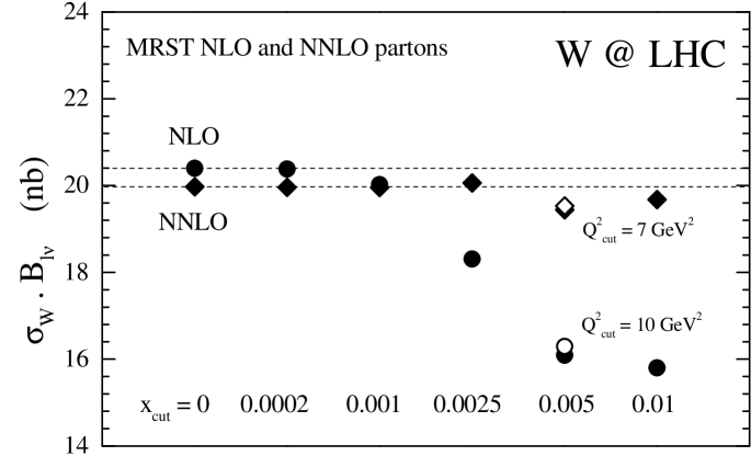
Figure 1: (a) Dependence of the MRST predictions for the total $W$ production cross section at the LHC on kinematic cuts on input data used in the global analysis; (b) the $W$ rapidity distribution according to the MRST default PDFs, and the “conservative” PDFs (based on relatively high $x$ and $Q$ cuts). Both figures are reproduced from [4].

Figure 1(b) shows the predicted rapidity distributions for the $W$ boson. The prediction from the “conservative fit” (the one with the largest $x$ cut) drops steeply compared to that of the standard fit outside the central rapidity region, thus creating the drop in $\sigma_{W}$ seen in Fig. 1(a). This effect was attributed in Ref. [4] to a “tension” between the Tevatron inclusive jet data and the DIS data at small $x$ (HERA) and medium $x$ (NMC). That tension is gradually relaxed as the $x$ cut is raised, i.e., as more small-$x$ data are excluded. Evidently, removing the HERA constraint, and thus effectively placing more emphasis on the inclusive jet data, significantly changes the PDFs and the resulting prediction for $\sigma_{W}$. In the MRST analysis, the combined data also pull the gluon distribution to negative values at small $x$ and small $Q$. It is likely that these two problems—the instability of the prediction on $\sigma_{W}$ and the negative gluon PDF—are interrelated.

The CTEQ and MRST analyses use largely the same data sets, theory input and methodology. Hence they usually yield results that are in general agreement. However, minor differences between the choices made for these inputs can, under some circumstances, give rise to significant differences in the resulting PDFs and their predictions. For example, in Fig. 2(a) the fractional uncertainty of the $u$ quark distribution at $Q^{2}=10\,\mathrm{GeV}^{2}$, normalized to CTEQ6.1M [8], is shown as the shaded band for $10^{-4}<x<0.9$. The comparison curves are CTEQ6M [9], MRST2002 [10], MRST2003c [4], and the reference CTEQ6.1M (horizontal line). We see that: (i) the uncertainty is small, $\sim\!5\%$ for much of the $x$ range; and (ii) with the exception of MRST2003c (“c” for conservative) at small $x$, the fits agree reasonably well. This reflects the tight constraints imposed mainly by the precise DIS and DY data.

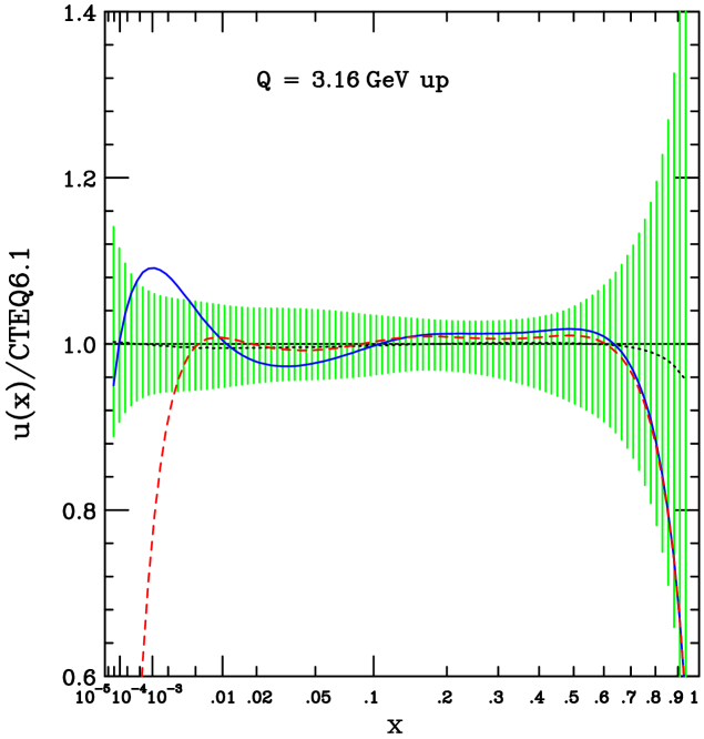
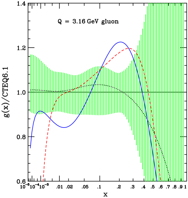
Figure 2: Comparison of CTEQ and MRST PDFs, for (a) the u-quark and (b) the gluon distributions at $Q^{2}=10\,\mathrm{GeV}^{2}$. The $x$ scale is chosen $\propto x^{1/3}$ to show details from both small- and large-$x$ regions clearly. The vertical axis is the ratio of the specified PDF set to CTEQ6.1M. The dotted curve is CTEQ6; solid curve is MRST2002; dashed curve is MRST2003c.

The corresponding comparison for the gluon distribution is shown in Fig. 2(b). We see that the fractional uncertainty is much larger in this case, especially for $x>0.25$. Even taking into account the size of the uncertainties, a difference in shape between the MRST and CTEQ gluon distributions over the full range of $x$ is evident. The differences between the MRST and CTEQ standard fits indicate how the small-to-medium-$x$ DIS data and the medium-to-large-$x$ Tevatron inclusive jet data are being fit differently in the two analyses (to be discussed below). Also noticeable is the change in shape of $g(x,Q)$ below $x\sim 0.1$ between the default and conservative MRST distributions. This difference shows the effect of cutting out DIS data at small $x$.

The gluon distribution is closely tied to the jet data. The stronger gluon at high $x$ in CTEQ6.1 leads to a larger predicted cross section at high jet $E_{T}$, in better agreement with the Tevatron data. Quantitatively, $\chi^{2}$ for the Tevatron Run 1 CDF and D0 jet data is 118 for 123 data points in the CTEQ6.1M fit. The corresponding numbers for MRST2002 are $\sim\!160$ for 115 data points [10, 4]. Figure 3 shows four $\eta$ bins of the D0 data, along with the theoretical curves obtained with CTEQ6.1M, MRST2002 and MRST2003c PDFs.

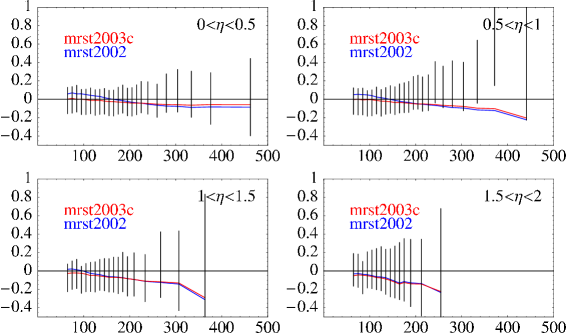
Figure 3: Comparison between the D0 jet data and cross sections calculated with CTEQ6.1 (horizontal line), MRST2002, and MSRT2003c PDFs. The vertical axis is the fractional difference (data-CTEQ6.1)/CTEQ6.1.

In the PDF parametrization adopted in the standard MRST fits, the rather high value of $\chi^{2}$ for the jet cross section results from a trade-off with the $\chi^{2}$ of DIS data at small-to-medium $x$ (hence the tension) [10, 4]. This tension is relaxed only when DIS data with $x<0.005$, and $Q^{2}<10\,\mathrm{GeV}^{2}$ are removed from the fit, resulting in the conservative fit MRST2003c, which reduces $\chi^{2}$ for the jet data sets significantly [4, 11]. The reduction in $\chi^{2}$ occurs mostly in the low transverse momentum range ($100-200\,\mathrm{GeV/c}$) for the lower rapidity bins: it results from an interaction between the change in the predicted jet cross section and the shapes of the experimental correlated systematic errors. These differences between the two fits are attributable mainly to differences in the gluon distribution. In contrast, in the CTEQ6.1 fits, the already good $\chi^{2}$ for the jet data does not improve noticeably when similar cuts are made (cf. Sec. 4).

The significant differences between the MRST standard and conservative fits, and their physical predictions (cf. Fig. 1), highlight the instability of these NLO QCD global analyses. The “conservative” fit, although free from apparent tension, is not to be considered a serious candidate for calculating safe physical predictions [4]. First, the removal of the high precision small-$x$ and low-$Q$ DIS data results in the loss of powerful constraints on the PDFs. Therefore the uncertainty is increased for physical predictions that depend on small-$x$ PDFs, which includes much of the physics at the LHC. Second, in the particular case of MRST2003c, the gluon distribution becomes strongly negative at small $x$ as seen in Fig. 10(a) of Appendix B. Therefore unphysical negative predictions result for some quantities, such as $F_{L}$ in DIS, and $d\sigma_{W}/dy$ at large $y$ for very high energies.

In the MRST analyses, NLO fits are unstable due to tension between the inclusive jet data and the DIS data. On the other hand, the CTEQ NLO global analyses do not show this tension. It is therefore important to investigate the stability issue in more detail within the CTEQ framework, to determine whether the NLO analysis is viable.

3 Inputs to the current analysis

The new global analyses in our stability study are extensions of the CTEQ6 analysis. We briefly summarize the theoretical and experimental inputs in this section. Some of these features are relevant for later discussions on the comparison of our results with those of Ref. [4]. For details, see the CTEQ6 paper [9].

We use the $\overline{\mathrm{MS}}$ scheme in the conventional PQCD framework, with three light quark flavors ($u,d,s$). The charm and bottom partons are turned on above momentum scales ($\mu_{f}=Q$) equal to the heavy quark masses $m_{c}=1.3\,\mathrm{GeV}$ and $m_{b}=4.5\,\mathrm{GeV}$. To be consistent with the most common applications of PDFs in collider phenomenology, each parton flavor is treated as massless above its mass threshold.

The input nonperturbative PDFs are defined at an initial scale $\mu_{f}=Q_{0}=1.3\,\mathrm{GeV}\ (=m_{c})$ using functional forms that meet certain criteria: (i) they must reflect qualitative physical behaviors expected at small $x$ (Regge behavior) and large $x$ (spectator counting rules); and (ii) they must be flexible enough to allow for unknown nonperturbative behavior (to be determined by fitting data); while (iii) they should not involve more free parameters than can be constrained by available data. In general, we use the functional form

$$xf(x,Q_{0})=A_{0}\,x^{A_{1}}\,(1-x)^{A_{2}}\,\mathrm{e}^{A_{3}\,x}\,(1+\mathrm{e}^{A_{4}}\,x)^{A_{5}}$$ (1)

for each flavor (see [9] for motivation and explanation). This generic form is modified as necessary to study specific issues—such as whether a negative gluon distribution at small $x$ is indicated by data.

The experimental data sets that are used in the new analyses are essentially the same as those of CTEQ6, with minor updates. As mentioned in the previous sections, kinematic cuts on the input data sets are systematically varied as a part of the stability study.

4 Results on the stability of NLO global analysis

The stability of our NLO global analysis is investigated by varying the inherent choices that must be made to perform the analysis. These choices include the selection of experimental data points based on kinematic cuts, the functional forms used to parametrize the initial nonperturbative parton distribution functions, and the treatment of $\alpha_{s}$. Sections 4.1–4.3 discuss the kinematic cuts and the form of the gluon distribution, which relate directly to the “tension” found in [4] that motivated this study. Section 4.4 discusses the role of different assumptions on $\alpha_{s}(Q)$.

The stability of the results is most conveniently measured by differences in the global $\chi^{2}$ for the relevant fits. To quantitatively define a change of $\chi^{2}$ that characterizes a significant change in the quality of the PDF fit is a difficult issue in global QCD analysis. In the context of the current analysis, we have argued that an increase by $\Delta\chi^{2}\sim 100$ (for $\sim$ ​ 2000 data points) represents roughly a 90% confidence level uncertainty on PDFs due to the uncertainties of the current input experimental data [13, 14, 15, 9]. In other words, PDFs with $\chi^{2}-\chi^{2}_{\mathrm{BestFit}}>100$ are regarded as not tolerated by current data. This tolerance will provide a useful yardstick for judging the significance of the fits in our stability study, because currently available experimental data cannot distinguish much finer differences.

4.1 Stability of global fits: Kinematic cuts on input data

The CTEQ6 and previous CTEQ global fits imposed “standard” cuts $Q>2\,\mathrm{GeV}$ and $W>3.5\,\mathrm{GeV}$ on the input data set, in order to suppress higher-order terms in the perturbative expansion and the effects of resummation and power-law (“higher twist”) corrections. We examine in this section the effect of stronger cuts on $Q$ to see if the fits are stable. We also examine the effect of imposing cuts on $x$, which should serve to suppress any errors due to deviations from DGLAP evolution, such as those predicted by BFKL. The idea is that any inconsistency in the global fit due to data points near the boundary of the accepted region will be revealed by an improvement in the fit to the data that remain after those near-boundary points have been removed. In other words, the decrease in $\chi^{2}$ for the subset of data that is retained, when the PDF shape parameters are refitted to that subset alone, measures the degree to which the fit to that subset was distorted in the original fit by compromises imposed by the data at low $x$ and/or low $Q$.

The main results of this study are presented in Table 1. Three fits are shown, from three choices of the exclusionary cuts on input data as specified in the table. They are labeled ‘standard’, ‘intermediate’ and ‘strong’. $N_{\rm pts}$ is the number of data points that pass the cuts in each case, and $\chi^{2}_{N_{\rm pts}}$ is the $\chi^{2}$ value for that subset of data. The fact that the changes in $\chi^{2}$ in each column are insignificant compared to the uncertainty tolerance is strong evidence that our NLO global fit results are very stable with respect to choices of kinematic cuts.

Cuts	$Q_{\mathrm{min}}$	$x_{\mathrm{min}}$	$N_{\mathrm{pts}}$	$\chi^{2}_{1926}$	$\chi^{2}_{1770}$	$\chi^{2}_{1588}$	$\sigma_{W}^{\mathrm{LHC}}\!\times\!B_{\ell\nu}\,[\mathrm{nb}]$
standard	$2\,\mathrm{GeV}$	$0$	$1926$	$2023$	$1850$	$1583$	$20.02$
intermediate	$2.5\,\mathrm{GeV}$	$0.001$	$1770$	–	$1849$	$1579$	$20.10$
strong	$3.162\,\mathrm{GeV}$	$0.005$	$1588$	–	–	$1573$	$20.34$

Table 1: Comparisons of three fits with different choices of the exclusionary cuts on input data at the $Q$ and $x$ values indicated. In these fits, a conventional positive-definite gluon parametrization was used.

As an example, note that the subset of 1588 data points that pass the strong cuts ($Q>3.162\,\mathrm{GeV}$ and $x>0.005$) are fit with $\chi^{2}\!=\!1573$ when fitted by themselves; whereas the compromises that are needed to fit the full standard data set force $\chi^{2}$ for this subset up to $1583$. This small increase—only $10$ in the total $\chi^{2}$ for this large subset—is an order of magnitude smaller than the increase that would represent a significant change in the quality of the fit according to our tolerance criterion for uncertainties.

4.2 Stability of global fits: negative gluon at small $x$?

We have extended the analysis to a series of fits in which the gluon distribution $g(x)$ is allowed to be negative at small $x$, at the scale $Q_{0}\!=\!1.3\,\mathrm{GeV}$ where we begin the DGLAP evolution. The purpose of this additional study is to determine whether the feature of a negative gluon PDF is a key element in the stability puzzle, as suggested by the findings of [4]. The results are presented in Table 2. Even in this extended case, we find no evidence of instability. For example, $\chi^{2}$ for the subset of 1588 points that pass the strong cuts increases only from 1570 to 1579 when the fit is extended to include the full standard data set.

Cuts	$Q_{\mathrm{min}}$	$x_{\mathrm{min}}$	$N_{\mathrm{pts}}$	$\chi^{2}_{1926}$	$\chi^{2}_{1770}$	$\chi^{2}_{1588}$	$\sigma_{W}^{\mathrm{LHC}}\!\times\!B_{\ell\nu}\,[\mathrm{nb}]$
standard	$2\,\mathrm{GeV}$	$0$	$1926$	$2011$	$1845$	$1579$	$19.94$
intermediate	$2.5\,\mathrm{GeV}$	$0.001$	$1770$	–	$1838$	$1574$	$19.80$
strong	$3.162\,\mathrm{GeV}$	$0.005$	$1588$	–	–	$1570$	$19.15$

Table 2: Same as Table 1 except that the gluon parametrization is extended to allow negative values.

Comparing the elements of Table 1 and Table 2 shows that our fits with $g(x)<0$ have slightly smaller values of $\chi^{2}$: e.g., $2011$ versus $2023$ for the standard cuts. However, the difference $\Delta\chi^{2}\!=\!12$ between these values is again not significant according to our tolerance criterion.

Negative parton distributions in a given renormalization and factorization scheme are not strictly forbidden by theory. However, a PDF set that leads to any negative cross sections—either of practical importance or as a matter of principle—must be regarded as unphysical. Therefore to establish the viability of a PDF set with negative PDFs is very difficult: the negative PDFs can be enhanced in a special kinematic region for a specific cross section, leading to a negative cross section.

Our results from a parametrization that allows $g(x)<0$ lead us to conclude that a negative gluon distribution may be permitted, but is certainly not mandated, by our analysis. Further discussion of this point, with specific examples from our fits and those of [4], is contained in Appendix B.

4.3 Stability of physical predictions

The last columns of Tables 1 and 2 show the predicted cross section for $W^{+}+W^{-}$ production at the LHC. This prediction is also very stable: it changes by only $1.6\%$ for the positive-definite gluon parametrization, which is substantially less than the overall PDF uncertainty of $\sigma_{W}$ estimated previously with the standard cuts. For the negative gluon parametrization, the change is $4\%$—larger, but still less than the overall PDF uncertainty. These results are explicitly displayed, and compared to the MRST results of Fig. 1, in Fig. 4.

Figure 4: Predicted total cross section of $W^{+}+W^{-}$ production at the LHC for the fits obtained in our stability study, compared to the NLO results of Ref. [4] (cf. Fig. 1). The $Q$-cut values associated with the CTEQ points are given in the two tables. The overall PDF uncertainty of the prediction is $\sim 5\%$.

We see that this physical prediction is indeed insensitive to the kinematic cuts used for the fits, and to the assumption on the positive definiteness of the gluon distribution. We have obtained similar results (not shown) for the individual $W^{+}$ and $W^{-}$ cross sections at the LHC and at the Tevatron. A more focused study on the uncertainty of the LHC prediction and its variation with the kinematic cuts, using the Lagrange Multiplier method, is given in Sec. 5.

This section has demonstrated stability of our NLO global fits with respect to cuts on $x$ and $Q$ and with respect to the parametrization of the gluon input. This result is consistent with the expected numerical accuracy of the PQCD expansion. However, it is in apparent disagreement with the findings of [4]. The two analyses have some other differences, including the treatment of $\alpha_{s}$ which we examine next.

4.4 Stability and $\alpha_{s}$

The CTEQ5/6/6.1 PDF sets were extracted assuming $\alpha_{s}(m_{Z})=0.118\,$. This value was chosen to approximate the world average, thereby to incorporate the rather strong constraints from measurements—especially from LEP—that are not otherwise included in our input data set. To examine the influence of $\alpha_{s}(m_{Z})$ on the quality and stability of the fit, we have made a series of fits with different choices for $\alpha_{s}(m_{Z})$. This exercise provides a further test of the reliability of our analysis.

The results for $\chi^{2}$ as a function of $\alpha_{s}(m_{Z})$ take the parabolic form shown as the solid curve in Fig. 5(a).

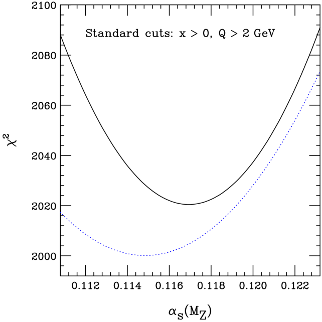
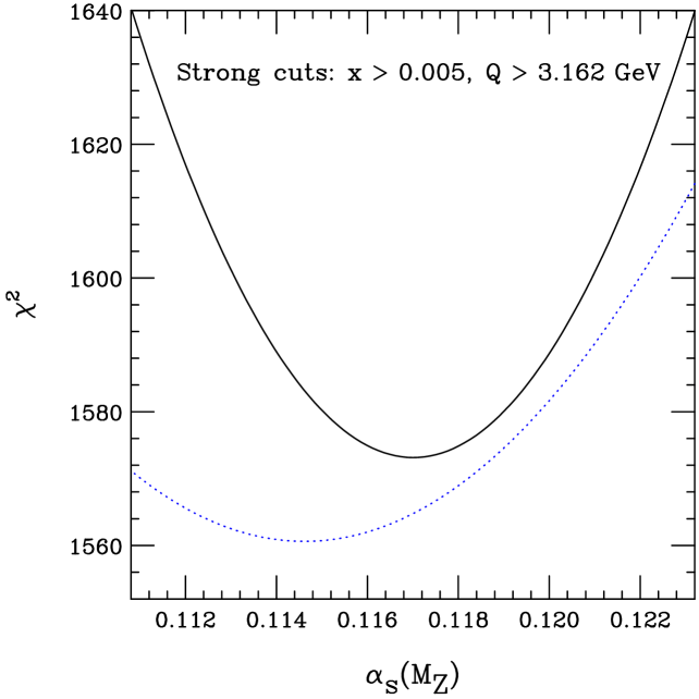
Figure 5: (a) The global fit $\chi^{2}$ as a function of $\alpha_{s}(m_{Z})$ using the standard data cuts. The solid curve assumes $g(x)>0$; the dotted curve allows $g(x)<0$. (b) Analogous curves using the strong data cuts.

Qualitatively, the value of $\alpha_{s}(m_{Z})$ preferred by the global fit is in reasonable agreement with the World Average, which lends support to the idea that NLO QCD is working successfully in the global fit. To obtain a quantitative result, we assume that $\Delta\chi^{2}=37$ defines a $1\,\sigma$ error (based on the estimated 90% C.L. range for $\Delta\chi^{2}=100$ mentioned previously). In this way we obtain

$$\alpha_{s}(m_{Z})=0.1169\pm 0.0045\;(0.1148\pm 0.0050)$$ (2)

from the PDF fit using the standard data cuts, assuming $g(x)\!>\!0$ ($g(x)\!<\!0$ allowed). These results are fully consistent with the current world average $0.1187\pm 0.0020$[16], or with the LEP QCD working group average $0.1201\pm 0.0003\pm 0.0048$. This consistency lends confidence to the standard analysis—including the “standard” data cuts used in it. The average $\chi^{2}$ per data point at the minimum, $\chi^{2}/N=2020/1926=1.049$ for the standard cut fit, is also comfortably close to $1$.

The solid curve in Fig. 5(b) shows the effect of imposing the “strong” data cuts ($Q>3.162\,\mathrm{GeV}$, $x>0.005$). The allowed range in $\chi^{2}$ should scale as the number of data points, so we estimate the $1\,\sigma$ uncertainty range in the case of the strong cuts as the range over which $\chi^{2}$ increases by $37\times(1588/1926)$ above its minimum value. This leads to

$$\alpha_{s}(m_{Z})=0.1168\pm 0.0044\;(0.1159\pm 0.0051)$$ (3)

from the PDF fit using the strong data cuts, assuming $g(x)\!>\!0$ ($g(x)\!<\!0$ allowed). The similarity between this result and Eq. (2) shows that the fit is very stable with respect to the cuts.

The dotted curves in Fig. 5 show the effect of allowing the gluon distribution $g(x,Q_{0})$ to be negative at small $x$. The resulting uncertainties in $\alpha_{s}$ are somewhat larger than for the positive gluon cases. In addition, the minimum $\chi^{2}$ values are somewhat lower than for positive-definite gluons. However, in view of the larger number of degrees of freedom in the fit and the reservations expressed previously concerning negative parton distributions, we do not consider these differences in minimum $\chi^{2}$ persuasive.

In addition to the possible range of values of $\alpha_{s}(m_{Z})$, there is an uncertainty caused by ambiguity in how to define $\alpha_{s}(Q)$ at NLO. We show in Appendix A that this ambiguity also has little effect on the results of the global fits or their stability.

4.5 Comments and Discussion

The results for $\chi^{2}_{1770}$ and $\chi^{2}_{1588}$ in Tables 1 and 2, and the results on $\sigma_{W}^{\mathrm{LHC}}$ given in those Tables and in Fig. 4 show a reassuring stability of the global fits. This confirms the general expectations for the PQCD expansion, and lends confidence to the extensive body of NLO phenomenological work that is being done in connection with current and future collider physics programs. However, it is important to ask why our results differ from those of [4]. Two separate issues are involved in the comparison between the two global analysis programs.

First, the instability of the NLO analysis observed in [4] appeared originally to result from a “tension” between the Tevatron inclusive jet data (mostly at medium and large $x$) and the DIS data at small and medium $x$. This tension has been a persistent feature of recent MRST analyses. However, CTEQ analyses, including the current study, have consistently not seen it. The difference appears to be due to the behavior of the gluon distribution at large $x$. The CTEQ input gluon distribution is consistently higher in the large $x$ region, which produces a much better fit to the CDF and D0 jet production cross section without affecting the fits to the DIS data. This point has been confirmed recently by a new MRST paper [11], which uses an input gluon distribution quite similar in shape to the CTEQ $g(x)$. The large-$x$ behavior of the relevant PDF sets in discussed in Appendix C.

The second issue concerns negative gluons at small $x$. Whereas we find only marginal differences in the quality of the global fits when the input gluon function is allowed to become negative, MRST has found a strong pull toward negative gluon in their analyses. Furthermore, their gluon distribution becomes increasingly negative as the $x$ cut is raised. The increasingly negative gluon distribution at small $x$, through its influence on the sea quark distributions via QCD evolution, is directly responsible for the rapid decrease of $d\sigma_{W}^{\mathrm{LHC}}/dy$ outside the central rapidity region, and the consequent decrease of the total $\sigma_{W}^{\mathrm{LHC}}$, as seen in Fig. 1. Further details on the small-$x$ behavior of the relevant PDFs are discussed in Appendix B.

The source of the different conclusions about a negative gluon PDF is tentatively identified in Appendix B as a difference in assumptions about the input gluon distribution. At any rate, because the improvement to the fit is small, and because of the reservations expressed earlier about negative PDFs, we do not believe that allowing negative gluons is necessary to the global analysis.

5 Stability and Uncertainty of $\sigma_{W}$ at the LHC

In this section, we study in detail the stability of the NLO prediction for the cross section $\sigma_{W}$ for $W^{+}+W^{-}$ production at the LHC, using the Lagrange Multiplier (LM) method of Refs. [13, 14, 15]. Specifically, we perform a series of fits to the global data set that are constrained to specific values of $\sigma_{W}$ close to the best-fit prediction. The resulting variation of $\chi^{2}$ versus $\sigma_{W}$ measures the uncertainty of the prediction. We repeat the constrained fits for each case of fitting choices (parametrization and kinematic cuts). In this way we gain an understanding of the stability of the uncertainty, in addition to the stability of the central prediction. The LM method is more robust than simply using the 40 eigenvector sets from CTEQ6.1, which were obtained using the Hessian method, because the LM technique probes the full parameter space instead of only the subspace of 20 free parameters that were varied in the Hessian method. We find that the uncertainty range obtained by the LM method is not much different from that obtained from the 40 sets, which demonstrates that the Hessian estimate of the uncertainty is not biased by choices made in the parametrizations at $Q_{0}$.

Figure 6 shows the results of the LM study for the three sets of kinematic cuts described in Table 1, all of which have a positive-definite gluon distribution.

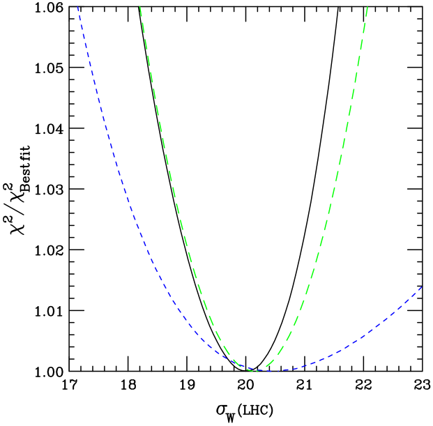
Figure 6: Lagrange multiplier results for the $W$ cross section (in $\mathrm{nb}$) at the LHC using a positive-definite gluon. The three curves, in order of decreasing steepness, correspond to the three sets of kinematic cuts labeled standard/intermediate/strong in Table 1.

The $\chi^{2}$ shown along the vertical axis is normalized to its value for the best fit in each series. In all three series, $\chi^{2}$ depends almost quadratically on $\sigma_{W}$. We observe several features:

• The location of the minimum of each curve represents the best-fit prediction for $\sigma_{W}^{\mathrm{LHC}}$ for the corresponding choice of exclusionary cuts. The fact that the three minima are close together displays the stability of the predicted cross section already seen in Table 1.

• Although more restrictive cuts make the global fit less sensitive to possible contributions from resummation, power-law and other nonperturbative effects, the loss of constraints caused by the removal of precision HERA data points at small $x$ and low $Q$ results directly in increased uncertainties on the PDF parameters and their physical predictions. This is shown in Fig. 6 by the increase of the width of the curves with stronger cuts. The uncertainty of the predicted $\sigma_{W}$ increases by more than a factor of 2 in going from the standard cuts to the strong cuts.

• The uncertainty range for $\sigma_{W}$ calculated from the 40 eigenvector uncertainty sets of CTEQ6.1 is $\pm 5.5\,\%$. The width of the $\chi^{2}$ parabola in Fig. 6 at $\Delta\chi^{2}=100$ for the standard cuts is similar, though it is slightly larger because the experimental normalizations, and all of the PDF shape parameters rather than just 20 of them, are treated as free in the LM fits. The LM method thus confirms that the estimate based on the eigenvector sets is reasonably good.

Figure 7(a) shows the results for the cases of standard/intermediate/strong cuts summarized in Table 2 when the gluon distribution is allowed to be negative at small $Q$ and $x$.

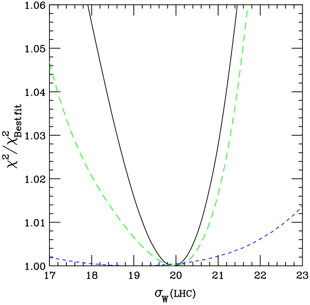
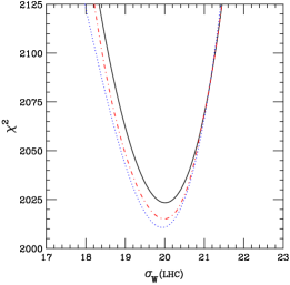
Figure 7: (a) LM results for the $W$ cross section at the LHC allowing negative gluon. The three curves, in order of decreasing steepness, correspond to the sets of kinematic cuts labeled standard/intermediate/strong in Table 2. (b) Comparison of the two cases of standard cuts: with (solid) or without (dotted) restricting the gluon to be positive definite. The negative gluon fit is slightly lower at the minimum, but the difference is not significant. The dot-dash curve is obtained by modifying the gluon parametrization in a manner that can suppress $g(x,Q_{0})$ at small $x$ without allowing it to become negative.

In this case, we observe:

• The stability of the best fits, represented by the minima of the curves, is again apparent.

• With strong cuts and allowing negative gluons, the uncertainty range of $\sigma_{W}$ expands considerably, especially toward low values of $\sigma_{W}$. The solutions at the extreme low end of the $\sigma_{W}$ range are most likely unphysical, since a strongly negative gluon distribution at small $x$ and $Q$ can drive the quark distributions negative at $x\sim 10^{-4}$ at moderate values of $Q$ by QCD evolution (cf. Appendix B).

Figure 7(b) compares the two LM series obtained using the standard cuts, with and without the positive definiteness requirement. We observe:

• Removing the positive definiteness condition necessarily lowers the value of $\chi^{2}$, because more possibilities are opened up in the $\chi^{2}$ minimization procedure. But the decrease is insignificant compared to other sources of uncertainty. Thus, a negative gluon PDF is allowed, but not required.

• The minima of the two curves occur at approximately the same $\sigma_{W}$. Allowing a negative gluon makes no significant change in the central prediction—merely a decrease of about $1\,\%$, which is small compared to the overall PDF uncertainty.

• For the standard set of cuts, allowing a negative gluon PDF would expand the uncertainty range only slightly.

• The dot-dash curve in Fig. 7(b) is obtained by modifying the gluon parametrization at $Q_{0}$ by including a factor $e^{-(a/x)^{b}}$, which can suppress $g(x,Q_{0})$ without allowing it to become negative. It demonstrates that most, if not all, of the reduction in $\chi^{2}$ obtainable by a low-$x$ suppression does not require $g(x)$ to be negative. We do not, however, find this small reduction in $\chi^{2}$ persuasive enough to give up the assumption of approximate Regge behavior at small $x$.

6 Conclusions

Motivated by its importance to all aspects of collider physics phenomenology at the Tevatron and the LHC, we have examined the stability of the NLO QCD global analysis with respect to certain variations in its input, in particular, the selection of input experimental data and the functional form of the nonperturbative gluon distribution.

As increasingly stringent kinematic cuts at higher $x$ and $Q$ are placed on the input data, in order to exclude potentially unsafe regions of phase space, we find no significant improvement in the quality of the fit, as measured by the $\chi^{2}$ of the retained data. In particular, we do not observe the “tension” discussed in recent MRST analyses. Simultaneous good fits to the HERA and Tevatron jet data are obtained for the full range of cuts explored. Predictions for the $W$ cross section at both the Tevatron and LHC were examined. As data at lower $x$ and $Q$ are removed from the analysis, the central value remains quite stable, while the uncertainty on the predicted $\sigma_{W}$ increases.

We have repeated this analysis with the gluon distribution allowed to assume negative values at small $x$. There is a slight reduction in the global $\chi^{2}$ (as is expected whenever the fitting parameter space is expanded), but the size of the reduction is too small to be of physical significance according to our analysis framework. As data at lower $x$ and $Q$ are removed, the central prediction for $\sigma_{W}$ again remains quite stable, while its uncertainty increases. In this case, when “strong” cuts in $x$ and $Q$ are made, similar to those of the MRST2003c “conservative” fit, the allowed range for $\sigma_{W}$ expands far enough to include the MRST2003c prediction. However it is not the central prediction, and we find no evidence of a tension between data sets that would support requiring such a strong cut; or support allowing a negative gluon distribution at small $x$. Thus we conclude that the predictions for $\sigma_{W}$ are sufficiently well defined that its use as luminosity monitor for QCD processes (“standard candle”) at the Tevatron and LHC is viable after all.

We have examined a number of aspects of our analysis that might account for the difference between our stability study and that of [4]. A likely candidate seems to be that in order to obtain stability, it is necessary to allow a rather free parametrization of the input gluon distribution. This suspicion is seconded by recent work by MRST [11], in which a different gluon parametrization appears to lead to a best-fit gluon distribution that is close to that of CTEQ6.

In summary, we have found that the NLO PDFs and their physical predictions at the Tevatron and LHC are quite stable with respect to variations of the kinematic cuts and the PDF parametrization after all. Thus, the NLO framework should provide sufficient accuracy for phenomenology at both Run II of the Tevatron and at the LHC. Further improvement will be possible with a NNLO global QCD analysis. A fully global analysis at NNLO, however, must wait for the completion of the NNLO QCD calculation of all of the relevant hard processes—in particular the inclusive jet cross section.

Acknowledgements:

We thank James Stirling and Robert Thorne for many informative and stimulating communications concerning the similarities and differences of the MRST and CTEQ analyses. This research is supported by the National Science Foundation.

Appendix A Definition of $\alpha_{s}(Q)$ at NLO

A subtle difference between various NLO global analyses arises from the choice of definition for the variation of $\alpha_{s}(Q)$ at NLO. The various choices differ only at NNLO, so a priori they are equally valid at NLO. Principal definitions in use are

1. Exact solution of the truncated renormalization group equation:

   $$\mu\,d\alpha/d\mu=c_{1}\alpha^{2}\,+\,c_{2}\alpha^{3}\;,$$ (4)

   where $c_{1}=-\beta_{0}/2\pi$ with $\beta_{0}=11-(2/3)\mathrm{n}_{f}$, and $c_{2}=-\beta_{1}/8\pi^{2}$ with $\beta_{1}=102-(38/3)\mathrm{n}_{f}$. This is the recipe used in the QCD evolution program QCDNUM [17], which is used by several groups, including ZEUS.

2. The original $\overline{\mathrm{MS}}$ definition at NLO [18]:

   $$\alpha(Q)=c_{3}\,[1-c_{4}\ln(L)/L]/L\;,$$ (5)

   where $L=\ln(Q^{2}/\Lambda^{2})$, $c_{3}=-2/c_{1}$, and $c_{4}=-2\,c_{2}/c_{1}^{2}\,$. This is the standard definition used in CTEQ global analyses.

3. The form chosen by MRST is less simple to state, since for $Q>m_{b}$ it contains a NNLO term that depends on $1/\alpha(m_{b})-1/\alpha(m_{c})$. However, it is numerically very similar to the QCDNUM choice.

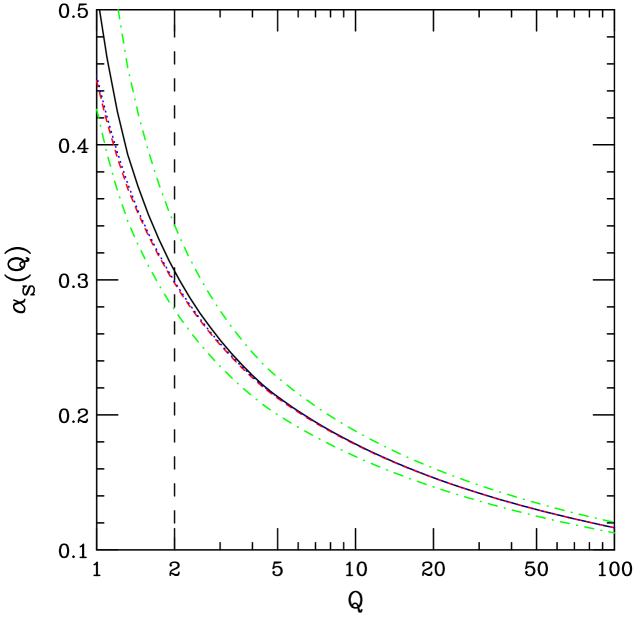
Figure 8: The dependence of $\alpha_{s}(Q)$ on $Q$. The solid curve is the CTEQ form; the dashed curve is the QCDNUM form; the dotted curve is the MRST form. These three curves all assume $\alpha_{s}(m_{Z})=0.118\,$. The dot-dash curves are the CTEQ form with $\alpha_{s}(M_{z})=0.114\,$, $0.122\,$.

Figure 8 shows that the MRST and QCDNUM forms are almost the same numerically; and that the difference between either of them and the CTEQ form is quite small in the region $Q>2\,\mathrm{GeV}$ where we fit data. In particular, that difference is much smaller than the difference caused by reasonable changes in $\alpha_{s}(M_{z})$.

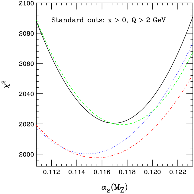
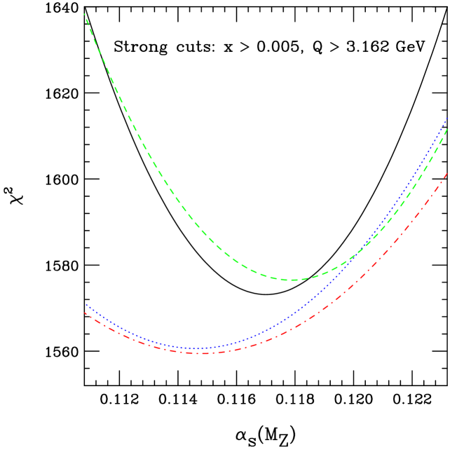
Figure 9: The global fit $\chi^{2}$ as a function of $\alpha_{s}(m_{Z})$ for (a) standard cuts, and (b) strong cuts. The solid curves use the CTEQ form for $\alpha_{s}(Q)$; the dashed curves use the QCDNUM form for it. These curves assume positive gluons; the corresponding curves with $g(x)<0$ allowed are dotted (CTEQ) and dot-dash (QCDNUM).

The dependence of $\chi^{2}$ for the global fit on $\alpha_{s}(m_{Z})$ is shown in Fig. 9 for standard and strong cuts. One sees that the choice of form for $\alpha_{s}(Q)$ has very little effect on the quality of the fit, which is a satisfying indication of the stability of the fit with respect to this arbitrary choice that must be made to carry it out. The similarity of the two figures shows that the fit is stable with respect to kinematic cuts as well.

In detail, the two choices produce somewhat different best-fit values for $\alpha_{s}(m_{Z})$. This can easily be understood using Fig. 8: for a given $\alpha_{s}(m_{Z})$, the QCDNUM choice gives a slightly smaller $\alpha_{s}(Q)$ in the region of $Q$—mostly much smaller than $m_{Z}$—that is important in the fit.

The uncertainties of $\alpha_{s}(Q)$ lead to an uncertainty in the prediction for $\sigma_{W}$ at the LHC. In particular, the four fits with standard cuts, which are shown in Fig. 9(a), span a range of $\pm 1.5\%$ ($\pm 2.9\%$) in $\sigma_{W}$ for $\alpha_{s}(m_{Z})=0.116$ – $0.120$ ($0.114$ – $0.122$). The four fits with strong cuts, shown in Fig. 9(b), span a much larger range: $\pm 8.2\%$ ($\pm 10.1\%$) in $\sigma_{W}$. Once again, we see the loss of predictive power when too much data is removed from the input.

Appendix B PDFs at small $x$: Do they go negative?

As mentioned in the text, the behavior of the gluon distribution (and through DGLAP evolution, the sea quark distributions) at small $x$ and low $Q$ appears to be an open issue at the present time. In particular, there is a question as to whether the data allow or suggest that these distributions become negative at small $x$. We discuss the situation in more detail in this appendix.

Figure 9 shows that allowing $g(x)<0$ (by inserting a factor $(1+ax^{b})$ into the standard CTEQ parametrization for $g(x)$ at $Q_{0}=1.3\,\mathrm{GeV}$, with $a$ and $b$ allowed to be negative) leads to a small improvement in the global fit: $\chi^{2}$ decreases by about $20$ (the difference between the minima of the solid and dotted curves in Fig. 9(a)). This decrease is well within the tolerance of our uncertainty range—especially in view of the fact that almost any additional freedom in the fitting functions is expected to permit at least a small decrease in $\chi^{2}$. The change in $\chi^{2}$ for the case of the strong data cuts (Fig. 9(b)) is about $13$—again not persuasive.

The MRST2003c NLO fit has a much more negative gluon than any of the fits described here, as shown in Fig. 10(a). Its negative region is so strong that it evolves to produce negative sea quark distributions for $x<2\times 10^{-5}$ at $Q=100\,\mathrm{GeV}$ (see Fig. 10(b)). The suppression of these sea quark distributions at small $x$ near where they pass through zero is responsible for the much smaller $\sigma_{W}$ ($16.12\,\mathrm{nb}$) predicted by the MRST2003c NLO PDFs, because $W$’s are produced at large rapidity by the annihilation of a quark at large $x$ with an antiquark at very small $x$. The small $x$ values are well below the $x$ cut on input data for the fit that created these PDFs, so the prediction is intrinsically unreliable. In fact, at a slightly higher energy, say $\sqrt{s}=40\,\mathrm{TeV}$, the same PDFs predict a negative cross section over a substantial region of large rapidity.

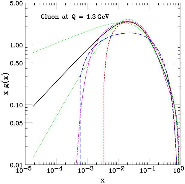
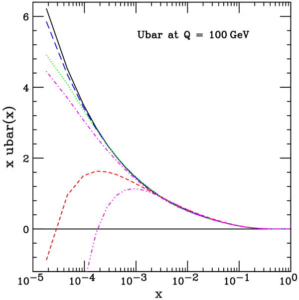
Figure 10: (a) Gluon distributions at $Q_{0}=1.3\,\mathrm{GeV}$ and (b) $\bar{u}(x)$ distributions at $Q=100\,\mathrm{GeV}$. The solid curves are CTEQ6.1; long dash curves are MRST2002; short dash curves are MRST2003c. In (a), the dotted curves are the two extremes from among the 40 eigenvector sets of CTEQ6.1; the dot-dash curve is discussed in footnote 12. In (b), the dotted curve has $g(x)<0$; dot-dash curve has $g(x)<0$ with $\sigma_{W}$ pushed small by LM with standard cuts; dot-dot-dash has $g(x)<0$ with $\sigma_{W}$ pushed small with strong cuts.

We are able to reproduce a similar suppression of the predicted $\sigma_{W}$ in our fits that allow a negative $g(x)$ at $Q_{0}$ only by simultaneously (1) imposing the strong data cuts on $x$ and $Q$; and (2) increasing the fit $\chi^{2}$ by $\sim\!20$ units by employing the Lagrange Multiplier method to force $\sigma_{W}$ downward. This modest increase in $\chi^{2}$ is acceptable according to our tolerance criterion. However, the stability of our fits with respect to the cuts makes it unnatural to impose the strong cuts. And, as mentioned above, these PDFs should not be trusted in the first place, in the small-$x$ region that lies below the $x$ cut on the data input to the fit.

Figure 10(b) shows the $\bar{u}(x)$ distribution at $Q=100\,\mathrm{GeV}$. (The $u(x)$, $d(x)$, $\bar{u}(x)$, $\bar{d}(x)$ are nearly identical at small $x$.) The CTEQ6.1 and MRST2002 curves are very similar, while MRST2003c turns negative at small $x$. Our best fit with $g(x)<0$ is quite similar to CTEQ6.1. Even when $\sigma_{W}$ is forced smaller by a Lagrange multiplier that raises $\chi^{2}$ by $70$, the distribution is not greatly different. Substantially different behavior is obtained only when we impose the strong data cuts and force $\sigma_{W}$ small by a Lagrange multiplier (dot-dot-dash curve).

Appendix C Gluon distribution at large $x$: Do counting rules count?

The behavior of the gluon distribution at large $x$ strongly affects the fit to inclusive jet production data. It therefore has a direct bearing on whether the jet data can be described simultaneously with the precision DIS data.

Figure 11(a) shows the gluon distribution at $Q=100\,\mathrm{GeV}$ from various PDF fits. The solutions that fit the jet data best are those with a rather strong gluon at large $x$, such as CTEQ6.1 (the solid curve). The two dotted curves are eigenvector sets 29 and 30, which are the members of the 40 eigenvector uncertainty PDF sets that have the most extreme gluon distributions [8]. MRST2002 lies just at the edge of this range of uncertainty, which presumably accounts for the “tension” MRST find between DIS and jets with this solution. MRST2003c is slightly closer to the CTEQ result, while the most recent MRST2004 is much closer to it.

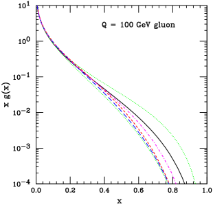
Figure 11: (a) Gluon at $Q=100\,\mathrm{GeV}$; and (b) gluon at $Q=1.3\,\mathrm{GeV}$. The solid curve is CTEQ6.1; the long dash curve is MRST2002; the short dash curve is MRST2003c; the dot-dash curve is MRST2004. The dotted curves are the extreme gluon distributions (sets 29 and 30) from among the 40 uncertainty eigenvector sets.

In all PDF analyses, the gluon distribution at $Q_{0}$ has been parametrized in a form that varies as $(1-x)^{a}$ as $x\to 1$. We have treated $a$ as a free parameter in the fitting, just like all of the other parton shape parameters at $Q_{0}=1.3\,\mathrm{GeV}$. Fig. 11(b) shows the gluon distributions as a function of $1-x$ on a log-log plot. The approximately straight-line behavior at small $1-x$ shows that an effective $(1-x)^{a}$ dependence survives the effects of the other parameters. From the slopes of the straight lines, we find that the effective power $a$ is about $1.7$ for CTEQ6.1, and varies from $0.8$ to $3.6$ over the 40 eigenvector sets. This parameter is therefore not strongly constrained by the global fit; though it tends to be smaller than one would have expected on the basis of the “spectator counting rules,” [19] which predict a faster fall-off for gluons than for valence quarks at $x\to 1$.

The MRST2003c gluon has $a\approx 3.5$, similar to the steepest fall-off of the 40 uncertainty sets of CTEQ6.1. MRST2002 is even steeper, with $a\approx 4.1$. This difference between the MRST and CTEQ fits does not result directly from an attempt to satisfy the counting rules, since the parameter $a$ is treated as free in both fits. But the form of parametrization used in MRST2003c may tie the $x\to 1$ behavior more closely to the behavior at intermediate $x$, and in that way not allow $a$ to come out small.

Theoretical constraints for the parametrization of nonperturbative input parton distributions at small $x$ (Regge behavior) and large $x$ (spectator counting rules) are, at best, only qualitative guides, since there is no reason to impose the suggested behavior at any particular scale $Q_{0}$, nor for PDFs in any particular factorization scheme. Constraints imposed with one choice of scale and scheme can become rather different at another scale and scheme. In particular, the power $a$ of the $(1-x)^{a}$ factor for the input gluon distribution is well-known to be quite sensitive to the choice of factorization scheme.A recent paper by MRST [11] takes advantage of this feature, and obtains a much better fit to the inclusive jet data with a gluon parametrization in the DIS scheme that is close to the counting rule value (and similar to what they had used before in the $\overline{\mathrm{MS}}$ scheme). The resulting $g(x,Q_{0})$ in the $\overline{\mathrm{MS}}$ scheme, as shown in Fig. 11, turns out to be essentially similar to that of the CTEQ analyses, which was arrived at in the global fit by an unconstrained parametrization. The fact that the mrst2002 fit, which used a supposedly unconstrained model for the input $g(x)$, was improved by imposing an additional condition on the large-$x$ behavior of $g(x)$ suggests that the original parametrization was not sufficiently flexible.

By contrast, it is interesting to note that the large-$x$ valence quark behavior is expected to be relatively insensitive to the choice of scheme (cf. footnote 13). Phenomenologically, the powers $a$ for both the $u_{\mathrm{val}}$ and $d_{\mathrm{val}}$ distributions are found to be quite stable, and their values, although slightly dependent on the choice of $Q_{0}$, are generally consistent with expectations from the counting rules. These results provide additional evidence that the underlying theoretical framework of global QCD analysis is physically sound.

References

- [1] S. Alekhin, [arXiv:hep-ph/0311184]; Phys. Rev. D 68, 014002 (2003) [arXiv:hep-ph/0211096].
- [2] A. D. Martin, R. G. Roberts, W. J. Stirling and R. S. Thorne, Phys. Lett. B 531, 216 (2002) [arXiv:hep-ph/0201127].
- [3] S. Moch, J. A. M. Vermaseren and A. Vogt, A. Vogt, S. Moch, and J. A. M. Vermaseren, Nucl. Phys. B 691, 129 (2004) [arXiv:hep-ph/0404111].
- [4] A. D. Martin, R. G. Roberts, W. J. Stirling and R. S. Thorne, Eur. Phys. J. C 35, 325 (2004) [arXiv:hep-ph/0308087].
- [5] S. Chekanov et al. [ZEUS Collaboration], Phys. Rev. D 67, 012007 (2003) [arXiv:hep-ex/0208023].
- [6] C. Adloff et al. [H1 Collaboration], Eur. Phys. J. C 30, 1 (2003) [arXiv:hep-ex/0304003].
- [7] W. T. Giele, S. A. Keller and D. A. Kosower, [arXiv:hep-ph/0104052], unpublished.
- [8] D. Stump, J. Huston, J. Pumplin, W. K. Tung, H. L. Lai, S. Kuhlmann and J. F. Owens, JHEP 0310, 046 (2003) [arXiv:hep-ph/0303013].
- [9] J. Pumplin, D. R. Stump, J. Huston, H. L. Lai, P. Nadolsky and W. K. Tung, JHEP 0207, 012 (2002) [arXiv:hep-ph/0201195].
- [10] A. D. Martin, R. G. Roberts, W. J. Stirling and R. S. Thorne, Eur. Phys. J. C 28, 455 (2003) [arXiv:hep-ph/0211080].
- [11] A. D. Martin, R. G. Roberts, W. J. Stirling and R. S. Thorne, Phys. Lett. B 604, 61 (2004) [arXiv:hep-ph/0410230].
- [12] C. Adloff et al. [H1 Collaboration], Eur. Phys. J. C 13, 609 (2000) [arXiv:hep-ex/9908059].
- [13] J. Pumplin, D. R. Stump and W. K. Tung, Phys. Rev. D 65, 014011 (2002) [arXiv:hep-ph/0008191].
- [14] D. Stump et al., Phys. Rev. D 65, 014012 (2002) [arXiv:hep-ph/0101051].
- [15] J. Pumplin et al., Phys. Rev. D 65, 014013 (2002) [arXiv:hep-ph/0101032].
- [16] S. Eidelman et al. [Particle Data Group], Phys. Lett. B 592, 1 (2004).
- [17] M. Botje, Eur. Phys. J. C 14, 285 (2000) [arXiv:hep-ph/9912439].
- [18] W. A. Bardeen, A. J. Buras, D. W. Duke and T. Muta, Phys. Rev. D 18, 3998 (1978).
- [19] S. J. Brodsky and I. A. Schmidt, Phys. Lett. B 234, 144 (1990); P. Hoyer, Acta Phys. Polon. B 23, 1145 (1992) [arXiv:hep-ph/9210267]; and references therein.
- [20] J. F. Owens and W. K. Tung, Ann. Rev. Nucl. Part. Sci. 42, 291 (1992).