Leptoquark Single and Pair production at LHC with CalcHEP/CompHEP in the complete model

Abstract:

We study combined leptoquark (${L\!\!Q}$) single and pair production at LHC at the level of detector simulation. A set of kinematical cuts to maximize significance for combined signal events has been worked out.

It was shown that combination of signatures from ${L\!\!Q}$ single and pair production not only significantly increases the LHC reach, but also allows us to give the correct signal interpretation. In particular, it was found that the LHC has potential to discover ${L\!\!Q}$ with a mass up to $1.2$ TeV and $1.5$ TeV for the case of scalar and vector ${L\!\!Q}$, respectively, and ${L\!\!Q}$ single production contributes about 30-50% to the total signal rate for ${L\!\!Q}-l-q$ coupling, taken equal to the electromagnetic coupling.

This work is based on an implementation of the most general form of scalar and vector ${L\!\!Q}$ interactions with quarks and gluons into CalcHEP/CompHEP packages. This implementation, which authors made publicly available, was one the most important aspects of the study.

1 Introduction

Boson fields mediating lepton-quark interactions naturally appear in various extensions of the Standard Model which is known to be theoretically incomplete. Leptoquarks appear in the framework of Grand Unified theories (GUT) where quarks and leptons are unified in one matter multiplet [1], in the SUSY models with R-parity violation (in this case the mediator of the lepton-quark interaction is a squark or a slepton), as well as in composite models of leptons and quarks [2].

In general, boson fields give rise to violation of the baryon and lepton numbers (leading to fast proton decay) and flavor changing neutral current(FCNC) processes which are strongly constrained by experiment. In principle, those bosons should be heavy ($\sim M_{Planck}\sim 10^{19}$ GeV) to suppress these unwelcome processes. On the other hand, fast proton decay and FCNC problems can be avoided if the boson mass even is of the order of the electroweak (EW) scale. In the case of leptoquarks (${L\!\!Q}$), which exclusively induce lepton-quark interactions, the problems above are solved: 1) the fast proton decay problem is absent, since leptoquarks conserve the baryon and lepton numbers (in the case of squarks mediating lepton-quarks interactions, in R-parity violating SUSY models, the proton decay is preserved when only one, lepton or baryon number is conserved); 2) the FCNC problem is also absent under the assumption of flavor diagonal form of leptoquark-lepton-quark (${L\!\!Q}-l-q$) interactions.

Numerous experimental ${L\!\!Q}$ searches at HERA (e.g. [3]) and at the Tevatron (for recent results see, e.g. [4] and references therein) gave no positive results so far and provided only limits on ${L\!\!Q}$ masses and ${L\!\!Q}$ couplings to leptons and quarks. Eventually, the CERN Large Hadron Collider (LHC) will be able to extend significantly the reach for ${L\!\!Q}$ masses and couplings (see, e.g. [5, 6, 7, 8, 9]). In [10, 11] it was shown that Next-to-Leading-Order (NLO) corrections to ${L\!\!Q}$ pair production are positive and non-negligible ( up to 20% at the Tevatron and up to 90% at the LHC) and lead to further extension of the collider reach in ${L\!\!Q}$ searches. Leptoquarks can be produced not only in pairs (from gluon splitting) but also as a single particle in association with lepton [12, 13, 14]. In [15] authors noticed the importance of the combination of ${L\!\!Q}$ single and pair production analysis for the Tevatron collider, which partially motivated the present study.

In this article, we perform a new detailed study of ${L\!\!Q}$ production and decay at LHC. There are several motivations for this work. Firstly, we stress the importance of the study of combined ${L\!\!Q}$ single and pair production, since both contribute to the same signature at the detector simulation level. Therefore, combination of signatures from ${L\!\!Q}$ single and pair production not only significantly increases the LHC reach, but also allows us to give the correct signal interpretation. Secondly, we study the complete set of ${L\!\!Q}$ interactions including scalar and vector ${L\!\!Q}$ production and decay. Finally, one should stress that this study is based on the implementation of the complete ${L\!\!Q}$ model including the most general form of scalar and vector ${L\!\!Q}$ interactions with quarks and gauge bosons (including gluons) into CalcHEP/CompHEP packages [21, 20]. This is one of the most important aspects of this work. Such an implementation allowed us to study the effect of vector ${L\!\!Q}$ interactions with gluons via anomalous couplings of the most general form.

This paper is organized as follows. In section 2, we describe the general effective Lagrangian used in our study, as well as the implementation of this Lagrangian into the CalcHEP/CompHEP software package. In section 3, we present signal rates for ${L\!\!Q}$ single and pair production at the LHC for the case of scalar and vector ${L\!\!Q}$. In section 4, we perform an analysis of signal versus background at the detector level. Finally, in section 5, we draw conclusions on LHC potential for leptoquarks search.

2 ${L\!\!Q}$ model and its implementation into CalcHEP/CompHEP packages

2.1 The model

Following [16, 17], we use an effective Lagrangian with the most general dimensionless, $SU(3)\times SU(2)\times U(1)$ invariant couplings of scalar and vector leptoquarks to leptons and quarks with lepton and baryon number conservation:

$${\cal L}={\cal L}^{f}_{|F|=0}+{\cal L}^{f}_{|F|=2}+{\cal L}^{V}$$ (1)

Lagrangian ${\cal L}^{f}_{|F|=0,2}$ describes Yukawa type interactions of ${L\!\!Q}$ with leptons and quarks (${L\!\!Q}-l-q$), changing the fermion number $F$ by 0 or 2, respectively, where $F=3B+L$,  $B$ is the baryon number and $L$ is the lepton number. ${\cal L}^{f}_{|F|=0,2}$ conserves the baryon and lepton numbers and has a flavor diagonal form:

$${\cal L}^{f}_{|F|=0} = (h_{2L}\bar{u}_{R}\ell_{L}+h_{2R}\bar{q}_{L}i\tau_{2}e_{R})R_{2}+\tilde{h}_{2L}\bar{d}_{R}\ell_{L}\tilde{R}_{2}$$ (2)

$$+ (h_{1L}\bar{q}_{L}\ell_{L}+h_{1R}\bar{d}_{R}\gamma^{\mu}e_{R})U_{1\mu}$$

$$+ \tilde{h}_{1R}\bar{u}_{R}\gamma^{\mu}e_{R}\tilde{U}_{1\mu}+h_{3L}\bar{q}_{L}\vec{\bf\tau}\gamma^{\mu}\ell_{L}\vec{U}_{3\mu}+h.c.,$$

$${\cal L}^{f}_{|F|=2} = (g_{1L}\bar{q}_{L}^{c}i\tau_{2}\ell_{L}+g_{1R}\bar{u}_{R}^{c}e_{R})S_{1}$$ (3)

$$+ \tilde{g}_{1R}\bar{d}_{R}^{c}e_{R}\tilde{S}_{1}+g_{3L}\bar{q}_{L}^{c}i\tau_{2}\vec{\tau}\ell_{L}\vec{S}_{3}$$

$$+ (g_{2L}\bar{d}_{R}^{c}\gamma^{\mu}\ell_{L}+g_{2R}\bar{q}_{L}^{c}\gamma^{\mu}e_{R})V_{2\mu}$$

$$+ \tilde{g}_{2}\bar{u}_{R}^{c}\gamma^{\mu}\ell_{L}\tilde{V}_{2\mu}+h.c.$$

where $\tau_{i}$ are the Pauli matrices, $q_{L}$ and $\ell_{L}$ are $SU(2)_{L}$ quark and lepton doublets, respectively and $u_{R}$, $d_{R}$, and $e_{R}$ are corresponding singlet fields; charged conjugated fields are denoted by $f^{c}=C\bar{f}^{T}$. We follow the ${L\!\!Q}$ classification from [17]. Table 1 summarizes the complete set of scalar and vector ${L\!\!Q}$ fields appearing in Eq. (2)-(3): $S_{1}$, $\tilde{S}_{1}$, $\vec{S}_{3}$, $R_{2}$, $\tilde{R}_{2}$, and $V_{2}^{\mu}$, $\tilde{V}_{2}^{\mu}$, $U_{1}^{\mu}$, $\tilde{U}_{1}^{\mu}$, $\vec{U}_{3}$, respectively. Scalar ($S_{1},\tilde{S}_{1},\vec{S}_{3},R_{2},\tilde{R}_{2}$) and vector ($V_{2}^{\mu},\tilde{V}_{2}^{\mu},U_{1}^{\mu},\tilde{U}_{1}^{\mu},\vec{U}_{3}$) ${L\!\!Q}$s have Yukawa-type couplings to quarks and leptons denoted by ($g_{1(L,R)},\tilde{g}_{1R},g_{3L},h_{2(L,R)},\tilde{h}_{2L}$) and ($g_{2(L,R)},\tilde{g}_{2R},h_{1(L,R)},\tilde{h}_{1R},h_{3L}$) respectively, in Eq. (2)-(3). Couplings appearing in the Feynman rules of ${L\!\!Q}-q-l$ (${L\!\!Q}-q-\nu$) interactions (which we denote by $\lambda_{L}(lq)$, $\lambda_{R}(lq)$ and $\lambda_{L}(\nu q)$) are trivial linear combinations of $g,h,\tilde{g},\tilde{h}$ couplings presented in Table 1. The table also presents a notation for ${L\!\!Q}$ names in the model realized in CalcHEP/CompHEP packages which we describe below.

									CalcHEP/
${L\!\!Q}$($\Phi$)	Spin	F	Color	$T_{3}$	$Q_{em}$	$\lambda_{L}(lq)$	$\lambda_{R}(lq)$	$\lambda_{L}(\nu q)$	CompHEP
									notation($\Phi/\overline{\Phi}$)
$S_{1}$	0	-2	$\bar{3}$	$0$	$+1/3$	$g_{1L}$	$g_{1R}$	$-g_{1L}$	S1	/	s1
$\tilde{S}_{1}$	0	-2	$\bar{3}$	$0$	$+4/3$	$0$	$\tilde{g}_{1R}$	$0$	ST	/	st
				$+1$	$+4/3$	$-\sqrt{2}g_{3L}$	$0$	$0$	SP	/	sp
$\vec{S}_{3}$	0	-2	$\bar{3}$	$0$	$+1/3$	$-g_{3L}$	$0$	$-g_{3L}$	S0	/	s0
				$-1$	$-2/3$	$0$	$0$	$\sqrt{2}g_{3L}$	SM	/	sm
				$1/2$	$+5/3$	$h_{2L}$	$h_{2R}$	$0$	rp	/	RP
${R}_{2}$	0	0	${3}$
				$-1/2$	$+2/3$	$0$	$-h_{2R}$	$h_{2L}$	rm	/	RM
				$+1/2$	$+2/3$	$\tilde{h}_{2L}$	$0$	$0$	tp	/	TP
$\tilde{R}_{2}$	0	0	${3}$
				$-1/2$	$-1/3$	$0$	$0$	$\tilde{h}_{2L}$	tm	/	TM
				$+1/2$	$+4/3$	${g}_{2L}$	$g_{2R}$	$0$	VP	/	vp
${V}_{2\mu}$	1	-2	$\bar{3}$
				$-1/2$	$+1/3$	$0$	$g_{2R}$	$g_{2L}$	VM	/	vm
				$+1/2$	$+1/3$	$\tilde{g}_{2L}$	$0$	$0$	WP	/	wp
$\tilde{V}_{2\mu}$	1	-2	$\bar{3}$
				$-1/2$	$-2/3$	$0$	$0$	$\tilde{g}_{2L}$	WM	/	wm
${U}_{1\mu}$	1	0	${3}$	$0$	$+2/3$	$h_{1L}$	$h_{1R}$	$h_{1L}$	u1	/	U1
$\tilde{U}_{1\mu}$	1	0	${3}$	$0$	$+5/3$	$0$	$\tilde{h}_{1R}$	$0$	ut	/	UT
				$+1$	$+5/3$	$\sqrt{2}h_{3L}$	$0$	$0$	up	/	UP
$\vec{U}_{3\mu}$	1	0	${3}$	$0$	$+2/3$	$-h_{3L}$	$0$	$h_{3L}$	u0	/	U0
				$-1$	$-1/3$	$0$	$0$	$\sqrt{2}h_{3L}$	um	/	UM

Table 1: Quantum numbers for the complete set of scalar and vector ${L\!\!Q}$ fields appearing in Eq. 2,3:    $S_{1}$, $\tilde{S}_{1}$, $\vec{S}_{3}$, $R_{2}$, $\tilde{R}_{2}$, and $V_{2}^{\mu}$, $\tilde{V}_{2}^{\mu}$, $U_{1}^{\mu}$, $\tilde{U}_{1}^{\mu}$, $\vec{U}_{3}$, respectively [17]. Also, ${L\!\!Q}$-lepton-quark couplings [$\lambda_{L}(lq)$, $\lambda_{R}(lq)$ and $\lambda_{L}(\nu q)$] and notation for ${L\!\!Q}$ names for the model realized in CalcHEP/CompHEP are presented. The particle-antiparticle convention is defined as: $\overline{\Phi}_{F=2}\rightarrow lq$ and $\overline{\Phi}_{F=0}\rightarrow l\bar{q}$.

The ${L\!\!Q}$ interactions with gauge bosons are described by ${\cal L}^{V}$, obey the $SU(3)_{c}\times SU(2)\times U(1)_{Y}$ Standard Model symmetry.

The ${L\!\!Q}-gluon$ interactions are described by the Lagrangian of the most general form [18] for the scalar and vector ${L\!\!Q}$ interactions, ${\cal L}_{S}^{g}$ and ${\cal L}_{V}^{g}$, respectively:

$${\cal L}_{S}^{g} = \sum_{scalars}\left[\left(D^{\mu}_{ij}\Phi^{j}\right)^{\dagger}\left(D_{\mu}^{ik}\Phi_{k}\right)-M_{S}^{2}\Phi^{i\dagger}\Phi_{i}\right],$$ (4)

$${\cal L}_{V}^{g} = \sum_{vectors}\left\{-\frac{1}{2}V^{i\dagger}_{\mu\nu}V^{\mu\nu}_{i}+M_{V}^{2}\Phi_{\mu}^{i\dagger}\Phi^{\mu}_{i}-ig_{s}\left[(1-\kappa_{G})\Phi_{\mu}^{i\dagger}t^{a}_{ij}\Phi_{\nu}^{j}{\cal G}^{\mu\nu}_{a}+\frac{\lambda_{G}}{M_{V}^{2}}V^{i\dagger}_{\sigma\mu}t^{a}_{ij}V_{\nu}^{j\mu}{\cal G}^{\nu\sigma}_{a}\right]\right\}.$$

Here, $g_{s}$ denotes the strong coupling constant, $t_{a}$ are the generators of $SU(3)_{c}$, $M_{S}$($M_{V}$) are the scalar(vector) leptoquark masses, while $\kappa_{G}$ and $\lambda_{G}$ are the anomalous couplings related to the anomalous magnetic and quadrupole moments of vector ${L\!\!Q}$ [18]. Fields $\Phi$ and $\Phi^{\mu}$ represent scalar and vector leptoquarks, respectively. The field strength tensors of the gluon and vector leptoquark fields are:

$${\cal G}_{\mu\nu}^{a} = \partial_{\mu}G_{\nu}^{a}-\partial_{\nu}G_{\mu}^{a}+g_{s}f^{abc}G_{\mu b}G_{\nu c},$$

$$V_{\mu\nu}^{i} = D_{\mu}^{ik}\Phi_{\nu k}-D_{\nu}^{ik}\Phi_{\mu k},$$ (6)

with the covariant derivative given by

$$D_{\mu}^{ij}=\partial_{\mu}\delta^{ij}-ig_{s}t_{a}^{ij}G^{a}_{\mu}.$$ (7)

We omit here the analogous $U(1)_{Y}\times SU(2)$ piece of gauge interactions since it is not relevant for our study of ${L\!\!Q}$ production at LHC, where (gauge boson – ${L\!\!Q}$) interactions are eventually gluon dominant.

2.2 ${L\!\!Q}$ color factorization and model implementation into CalcHEP/CompHEP

The appearance of vertex with 4 color particles can not be straightforwardly implemented into CalcHEP/CompHEP packages. The idea is to split 4-color interactions into 3-color vertices via the introduction of auxiliary ghosts fields.

It is well known that for $G\bar{q}q$ and $GGG$ QCD vertices their color structure is factorisable. For calculation of Feynman diagrams with such vertices, where color indexes can be convolved separately, an elegant technique is presented in [19]. However, for $4G$ vertex such a factorization is absent. To have color factorization in the case of $4G$ vertex one can split this vertex into $3G$ vertex by means of the auxiliary tensor field ${G_{t}}_{\mu\nu}$[20]. This field should have the point-like propagator

$$<0|T[{G_{t}}^{\mu_{1}\nu_{1}}_{\alpha_{1}}(p_{1}),\;{G_{t}}^{\mu_{2}\nu_{2}}_{\alpha_{2}}(p_{2})]|0>=\frac{1}{(2\pi)^{4}i}\;\delta(p_{1}+p_{2})\,\delta_{\alpha_{1}\alpha_{2}}g^{\mu_{1}\mu_{2}}\,g^{\nu_{1}\nu_{2}}\;.$$ (8)

and interact with gluons according to

$$S_{G_{t}GG}=\frac{i\,g}{\sqrt{2}}\int f^{\alpha}_{\beta\gamma}{{G_{t}}_{\alpha}}^{\mu\nu}(x)G^{\beta}_{\mu}(x)G^{\gamma}_{\nu}(x)d^{4}x$$ (9)

Graphically, it can be represented as

Figure 1: Splitting of a four-gluon vertex into three-gluon vertex.

This trick was successfully implemented in CompHEP/CalcHEP packages for QCD Lagrangian. However in the case of the interaction of vector leptoquarks with gluon [18] one needs to develop this technique further and find a general prescription for splitting of the arbitrary color structure. Such a prescription is described below. We consider separately cases of real (e.g. gluon) and complex (e.g. leptoquark) vector fields.

In the case of a real vector field $\Phi_{\mu}$ interacting with a gluon field $G_{\mu}$, the Lagrangian can be presented as

$$L=-\frac{1}{4}|\partial_{\mu}\Phi_{\nu}-\partial_{\nu}\Phi_{\mu}+\Upsilon_{\mu\nu}|^{2}+Int(\Upsilon(\Phi,G),\Phi,...)$$ (10)

where $\Upsilon_{\mu\nu}=g[\Phi_{\mu},G_{\nu}]$, $Int$ represents terms of gluon interaction with color matter realized via general derivative or the strength tensor $F_{\mu\nu}$. The color index of the gluon fields is omitted to simplify the expressions.

Now, we replace $\Upsilon_{\mu\nu}$ by an auxiliary field $T_{\mu\nu}$ and confine of $\Upsilon=T$ by means of a Lagrange multiplier $t^{\mu\nu}$. We apply this procedure for the $Int$ and $\Upsilon(\Phi,G)^{2}$ terms, keeping the linear $\Upsilon$ term as it is:

$$L = -\frac{1}{4}|\partial_{\mu}\Phi_{\nu}-\partial_{\nu}\Phi_{\mu}|^{2}-\frac{1}{2}(\partial_{\mu}\Phi_{\nu}-\partial_{\nu}\Phi_{\mu})\Upsilon(\Phi,G)^{\mu\nu}$$ (11)

$$-\frac{1}{4}T_{\mu\nu}T^{\mu\nu}+\frac{1}{2}t_{\mu\nu}(T^{\mu\nu}-\Upsilon(\Phi,G)^{\mu\nu})$$

$$+Int(\Upsilon\rightarrow X,\Phi,...)$$

Then, we perform the following substitution of variables

$${\Phi_{T}}_{\mu\nu}=(T_{\mu\nu}-t_{\mu\nu})/\sqrt{2}\ \ \ \mbox{and}\ \ \ {\Phi_{t}}_{\mu\nu}=i\cdot t_{\mu\nu}/\sqrt{2}$$ (12)

in order to obtain standard normalized quadratic forms for the auxiliary fields:

$$L = -\frac{1}{4}|\partial_{\mu}\Phi_{\nu}-\partial_{\nu}\Phi_{\mu}|^{2}-\frac{1}{2}(\partial_{\mu}\Phi_{\nu}-\partial_{\nu}G_{\mu})\Upsilon(\Phi,G)^{\mu\nu}$$ (13)

$$-\frac{1}{2}{\Phi_{T}}_{\mu\nu}{\Phi_{T}}^{\mu\nu}-\frac{1}{2}{\Phi_{t}}_{\mu\nu}{\Phi_{t}}^{\mu\nu}+{i\over\sqrt{2}}{\Phi_{t}}\Upsilon(\Phi,G)^{\mu\nu}$$

$$+Int(\Upsilon\rightarrow\sqrt{2}(\Phi_{T}-i\cdot\Phi_{t}),G,...)$$

In the case of QCD interaction with scalar and fermion fields, the $Int()$ term does not contain $\Upsilon$. Thus, the auxiliary field $T$ is free and can be omitted. Other terms produce the $3-gluon$ interaction, the point-like propagator (8), and the interaction of just one auxiliary tensor field $t$ with gluons  (9).

Lagrangian with a complex vector field $\Phi$ also can be represented in a color-factored form using the same trick. In a general case, it is given as:

$$L=-\frac{1}{2}|\partial_{\mu}\Phi_{\nu}-\partial_{\nu}\Phi_{\mu}+\Upsilon(\Phi,G)_{\mu\nu}|^{2}+Int(\Upsilon(\Phi,G),\Upsilon(\Phi,G)^{*},\Phi,\Phi^{*},...)$$ (14)

Following the procedure adopted with real vector field, we introduce two auxiliary fields $T_{\mu\nu}$ and $t_{\mu\nu}$ which are now complex. In terms of these fields, the Lagrangian becomes:

$$L = -\frac{1}{2}|\partial_{\mu}\Phi_{\nu}-\partial_{\nu}\Phi_{\mu}|^{2}-\frac{1}{2}(\partial_{\mu}\Phi_{\nu}^{*}-\partial_{\nu}\Phi_{\mu}^{*})\Upsilon(\Phi,G)^{\mu\nu}-\frac{1}{2}\Upsilon(\Phi,G)^{*}_{\mu\nu}(\partial^{\mu}V^{\nu}-\partial^{\nu}V^{\mu})$$ (15)

$$-\frac{1}{2}T_{\mu\nu}^{*}T^{\mu\nu}+\frac{1}{2}t_{\mu\nu}^{*}(T^{\mu\nu}-\Upsilon(\Phi,G)^{\mu\nu})+\frac{1}{2}(T_{\mu\nu}^{*}-\Upsilon(\Phi,G)_{\mu\nu}^{*})t^{\mu\nu}$$

$$+Int(\Upsilon\rightarrow T,\Upsilon(\Phi,G)^{*}\rightarrow T^{*}...)$$

To obtain a standard normalized quadratic form of auxiliary fields, one should perform the following variable substitutions:

$${\Phi_{T}}_{\mu\nu}=(T_{\mu\nu}-t_{\mu\nu})/\sqrt{2}\;,\;\;{\Phi_{T}}_{\mu\nu}^{*}=(T_{\mu\nu}^{*}-t_{\mu\nu}^{*})/\sqrt{2}$$

$${\Phi_{t}}_{\mu\nu}=i\cdot t_{\mu\nu}/\sqrt{2}\;,\;\;but!\;\;{\Phi_{t}}^{*}=i\cdot t_{\mu\nu}^{*}/\sqrt{2}\;;$$ (16)

Note that this transformation is realized through a non-analytic manner which is legal for functional integrals. Now, the Lagrangian in color-factorized form can be given as

$$L = -\frac{1}{2}|\partial_{\mu}\Phi_{\nu}-\partial_{\nu}\Phi_{\mu}|^{2}-\frac{1}{2}(\partial_{\mu}\Phi_{\nu}^{*}-\partial_{\nu}\Phi_{\mu}^{*})\Upsilon(\Phi,G)^{\mu\nu}-\frac{1}{2}\Upsilon(\Phi,G)^{*}_{\mu\nu}(\partial^{\mu}\Phi^{\nu}-\partial^{\nu}\Phi^{\mu})$$ (17)

$$-|\Phi_{T}|^{2}-|\Phi_{t}|^{2}+{i\over\sqrt{2}}{\Phi_{t}}_{\mu\nu}^{*}\Upsilon(\Phi,G)^{\mu\nu}+{i\over\sqrt{2}}\Upsilon(\Phi,G)_{\mu\nu}^{*}{\Phi_{t}}^{\mu\nu}$$

$$+Int(\Upsilon\rightarrow\sqrt{2}(\Phi_{T}-i\cdot\Phi_{t}),\Upsilon(\Phi,G)^{*}\rightarrow\sqrt{2}(\Phi_{T}^{*}-i\cdot\Phi_{t}^{*})...)$$

In particular, for the case of Lagrangian (2.1) one has

$$\Upsilon(\Phi,G)_{\mu\nu}=-ig(G_{\mu}\Phi_{\nu}-G_{\nu}\Phi_{\mu})$$ (18)

$$\Upsilon(\Phi,G)_{\mu\nu}^{*}=ig(G_{\mu}\Phi_{\nu}^{\dagger}-G_{\nu}\Phi_{\mu}^{\dagger})$$ (19)

$$Int(\Upsilon\rightarrow\sqrt{2}(\Phi_{T}-i\cdot\Phi_{t}),\Upsilon(\Phi,G)^{*}\rightarrow\sqrt{2}(\Phi_{T}^{*}-i\cdot\Phi_{t}^{*})...)=$$

$$-ig(1-\kappa_{G})\Phi_{\mu}t^{a}\Phi_{\nu}[\partial_{\mu}G_{\nu}^{a}-\partial_{\nu}G_{\mu}^{a}+\sqrt{2}({\Phi_{t}}_{\mu\nu}^{a}-i{\Phi_{T}}_{\mu\nu}^{a})]$$

$$-ig{\lambda_{G}\over M_{\Phi}^{2}}[{\partial_{\sigma}}{\Phi^{\dagger}}_{\mu}-{\partial_{\mu}}{\Phi^{\dagger}}_{\sigma}+\sqrt{2}({\Phi_{T}}_{\sigma\mu}^{*}-i{\Phi_{t}}_{\sigma\mu}^{*})]\times$$

$$[{\partial_{\nu}}{\Phi}^{\mu}-{\partial^{\mu}}{\Phi}_{\nu}+\sqrt{2}({\Phi_{T}}_{\nu}^{\mu}-i{\Phi_{t}}_{\nu}^{\mu})]\times[({\partial^{\nu}}G^{\sigma}-{\partial^{\sigma}}G^{\nu}+\sqrt{2}({G_{T}}^{\nu\sigma}-i{G_{t}}^{\nu\sigma})]$$ (20)

In the case of a complex scalar field one should introduce two auxiliary vector fields – $V_{\mu}$ and $v_{\mu}$ (analogous to $T_{\mu\nu}$ and $t_{\mu\nu}$ tensors). The Lagrangian with the complex scalar field $\Phi$ can be represented as:

$$L=|\partial_{\mu}\Phi+\Upsilon(\Phi,G)_{\mu}|^{2}+Int(\Upsilon(\Phi,G),\Upsilon(\Phi,G)^{*},\Phi,\Phi^{*},...)$$ (21)

In terms of these fields, in exact analogy with the vector leptoquark field, we have

$$L = |\partial_{\mu}\Phi|^{2}+\partial_{\mu}\Phi^{*}\Upsilon(\Phi,G)^{\mu}+\Upsilon(\Phi,G)^{*}_{\mu}\partial^{\mu}\Phi$$ (22)

$$+V_{\mu}^{*}V^{\mu}-v_{\mu}^{*}[V^{\mu}-\Upsilon(\Phi,G)^{\mu}]-[V_{\mu}^{*}-\Upsilon(\Phi,G)_{\mu}^{*}]v^{\mu}$$

$$+Int(\Upsilon\rightarrow V,\Upsilon(\Phi,G)^{*}\rightarrow V^{*}...)$$

with the same variable substitutions:

$${\Phi_{V}}_{\mu}=(V_{\mu}-v_{\mu})/\sqrt{2} {\Phi_{V}}_{\mu}^{*}=(V_{\mu}^{*}-v_{\mu}^{*})/\sqrt{2}$$

$${\Phi_{v}}_{\mu}=i\cdot v_{\mu}/\sqrt{2} \ \ but!\ \ {\Phi_{v}}^{*}=i\cdot v_{\mu\nu}^{*}/\sqrt{2}$$ (23)

For Lagrangian (4) one has:

$$\Upsilon(\Phi,G)_{\mu}=-igG_{\mu}\Phi$$ (24)

$$\Upsilon(\Phi,G)_{\mu}^{*}=igG_{\mu}\Phi$$ (25)

$$Int(\Upsilon\rightarrow\sqrt{2}(\Phi_{V}-i\cdot\Phi_{v}),\Upsilon(\Phi,G)^{*}\rightarrow\sqrt{2}(\Phi_{V}^{*}-i\cdot\Phi_{v}^{*})...)=0.$$ (26)

P1   |P2   |P3   |  Factor              | Lorentz Part
---------------------------------------------------------------------------------------------
vm   |VM   |G    |  GG/MVM^2            |MVM^2*((1-KG)*(m2.p3*m1.m3-m1.p3*m2.m3)
                                        |     +(p2.m1*m2.m3-p1.m2*m1.m3+(p1-p2).m3*m1.m2))
                                        |      +LG*( p3.m1*(p1.m2*p2.m3-p1.p2*m2.m3)
                                        |           -p3.m2*(p1.m3*p2.m1-p1.p2*m1.m3)
                                        |           +p2.p3*(p1.m3*m1.m2-p1.m2*m1.m3)
                                        |          -p1.p3*(p2.m3*m1.m2-p2.m1*m2.m3))
vm   |VM.t |G    |  GG/MVM^2/Sqrt2      |MVM^2*( m1.m2*m3.M2-m1.M2*m3.m2)
                                        |+2*LG*( p3.m2*(p1.m3*m1.M2-p1.M2*m1.m3)
                                        |       +m3.m2*(p1.M2*p3.m1-p1.p3*m1.M2))
VM   |vm.t |G    | -GG/MVM^2/Sqrt2      |MVM^2*(m1.m2*m3.M2-m1.M2*m3.m2)
                                        |+2*LG*( p3.m2*(p1.m3*m1.M2-p1.M2*m1.m3)
                                        |        +m3.m2*(p1.M2*p3.m1-p1.p3*m1.M2))
vm   |VM.T |G    | i*GG/MVM^2*Sqrt2     |LG*( p3.m2*(p1.m3*m1.M2-p1.M2*m1.m3)
                                        |    +m3.m2*(p1.M2*p3.m1-p1.p3*m1.M2))
VM   |vm.T |G    |-i*GG/MVM^2*Sqrt2     |LG*( p3.m2*(p1.m3*m1.M2-p1.M2*m1.m3)
                                        |     +m3.m2*(p1.M2*p3.m1-p1.p3*m1.M2))
vm   |VM   |G.t  |  -GG*Sqrt2/MVM^2     |MVM^2*(1-KG)*m1.m3*m2.M3
                                        |-LG*( p1.M3*m1.m2*p2.m3-p1.m2*p2.m3*m1.M3
                                        |     -p1.M3*m2.m3*p2.m1+p1.p2*m1.M3*m2.m3)
vm   |VM   |G.T  |-i*GG*Sqrt2/MVM^2     |MVM^2*(1-KG)*m1.m3*m2.M3
                                        |-LG*( p1.M3*m1.m2*p2.m3-p1.m2*p2.m3*m1.M3
                                        |     -p1.M3*m2.m3*p2.m1+p1.p2*m1.M3*m2.m3)
vm   |VM.t |G.t  |   2*GG*LG/MVM^2      |m2.m3*(p1.M3*m1.M2-p1.M2*m1.M3)
vm   |VM.t |G.T  | 2*i*GG*LG/MVM^2      |m2.m3*(p1.M3*m1.M2-p1.M2*m1.M3)
vm   |VM.T |G.t  | 2*i*GG*LG/MVM^2      |m2.m3*(p1.M3*m1.M2-p1.M2*m1.M3)
vm   |VM.T |G.T  |  -2*GG*LG/MVM^2      |m2.m3*(p1.M3*m1.M2-p1.M2*m1.M3)
VM   |vm.t |G.t  |   2*GG*LG/MVM^2      |m2.M3*(p1.m3*m1.M2-p1.M2*m1.m3)
VM   |vm.t |G.T  | 2*i*GG*LG/MVM^2      |m2.M3*(p1.m3*m1.M2-p1.M2*m1.m3)
VM   |vm.T |G.t  | 2*i*GG*LG/MVM^2      |m2.M3*(p1.m3*m1.M2-p1.M2*m1.m3)
VM   |vm.T |G.T  |  -2*GG*LG/MVM^2      |m2.M3*(p1.m3*m1.M2-p1.M2*m1.m3)
vm.T |VM.T |G.T  |-i*GG*LG/MVM^2*2*Sqrt2| m1.M3*M1.M2*m2.m3
vm.t |VM.T |G.T  |  -GG*LG/MVM^2*2*Sqrt2| m1.M3*M1.M2*m2.m3
vm.T | VM.t|G.T  |  -GG*LG/MVM^2*2*Sqrt2| m1.M3*M1.M2*m2.m3
vm.t | VM.t|G.T  | i*GG*LG/MVM^2*2*Sqrt2| m1.M3*M1.M2*m2.m3
vm.T |VM.T |G.t  |  -GG*LG/MVM^2*2*Sqrt2| m1.M3*M1.M2*m2.m3
vm.t |VM.T |G.t  | i*GG*LG/MVM^2*2*Sqrt2| m1.M3*M1.M2*m2.m3
vm.T | VM.t|G.t  | i*GG*LG/MVM^2*2*Sqrt2| m1.M3*M1.M2*m2.m3
vm.t | VM.t|G.t  |   GG*LG/MVM^2*2*Sqrt2| m1.M3*M1.M2*m2.m3
vm.t | VM.t|G    | 2*GG*LG/MVM^2        | M1.M2*(p3.m2*m1.m3-p3.m1*m2.m3)
vm.T | VM.t|G    |2*i*GG*LG/MVM^2       | M1.M2*(p3.m2*m1.m3-p3.m1*m2.m3)
vm.t |VM.T |G    |2*i*GG*LG/MVM^2       | M1.M2*(p3.m2*m1.m3-p3.m1*m2.m3)
vm.T |VM.T |G    | -2*GG*LG/MVM^2       | M1.M2*(p3.m2*m1.m3-p3.m1*m2.m3)

Table 2: An example of the implementation of ${L\!\!Q}$ interactions with gluons in the CalcHEP/CompHEP packages for the case of $V_{2\mu}$ vector ${L\!\!Q}$ ($V\!M$) with $F=-2,T_{3}=-1/2,Q=+1/3$. See text for details.

One can see that the leptoquark Lagrangians given by Eq.(4)–(2.1) can be rewritten in terms of products of only three fields. The approach described above allows us to represent the strength tensor as a sum of vector fields and auxiliary tensor fields. Thus, interactions can be presented as a trilinear fields interaction only and, therefore, have simple unambiguously defined color factor that can be factorized.

As it was demonstrated above, the implementation of the complete ${L\!\!Q}$ model requires two auxiliary tensor fields $\Phi.t$ and $\Phi.T$ for each ${L\!\!Q}$ type. In CompHEP [20], only one tensor field ($\Phi.t$) is automatically generated, while CalcHEP [21] generates both of them. To implement the complete ${L\!\!Q}$ model into CompHEP one can introduce the second tensor field by doubling the vector ${L\!\!Q}$ fields (by introducing, say, $\tilde{\Phi}$ ${L\!\!Q}$ fields), and use the tensor field of those particles ($\tilde{\Phi}.t$) as a $\Phi.T$ field. The complete ${L\!\!Q}$ model given by Eq. (2)-(2.1) has been implemented and tested for both CompHEP and CalcHEP packages. The complete models of ${L\!\!Q}$ interactions relevant to LHC or Tevatron physics (i.e. models with ${L\!\!Q}-l-q$ and ${L\!\!Q}-gluon$ interactions) can be found at
http://hep.pa.msu.edu/belyaev/public/projects/lq/models/lq_calc.zip
and at
http://hep.pa.msu.edu/belyaev/public/projects/lq/models/lq_comp.zip
for CalcHEP and CompHEP, respectively. Results for ${L\!\!Q}$ pair production has been compared with those of paper [18]. We agree with the results of [18] except with the sign in front of $\lambda_{G}$ in the expression for vector ${L\!\!Q}$ pair production (for the sign convention defined by Eq. 2.1), which we found to be opposite in our calculations.

In Table 2, we present an explicit example of the implementation of ${L\!\!Q}$ interactions with gluons in the CalcHEP package for the case of $V_{2\mu}$ vector ${L\!\!Q}$ ($V\!M$) with $F=-2,T_{3}=-1/2,Q=+1/3$ (see Table 1). Table 2 is a piece of the CalcHEP model of particle interactions. The first three fields ‘$P1$’, ‘$P2$’ and ‘$P3$’ include the names of the interacting particles. The last two fields ‘Factor’ and ‘Lorentz Part’ define a vertex itself. Each line of the table represents a particles interaction vertex. Symbols ’up’, ’up.t’,’up.T’ correspond to a vector ${L\!\!Q}$, first tensor ${L\!\!Q}$ and second tensor ${L\!\!Q}$ fields, respectively. Names with capital letters: ‘UP’, ‘UP.t’,‘UP.T’ correspond to the hermitian conjugated fields. Gluon fields and its two tensor fields are denoted by ‘G’,‘G.t’,‘G.T’, respectively. The ‘Factor’ field contains ‘GG’, ‘MUP’, ‘LG’ and ‘Sqrt2’ which denote $g_{s}$, $M_{UP}$ (${L\!\!Q}$ mass), $\lambda_{G}$ and $\sqrt{2}$, respectively. Symbols ‘$mi.mj$’, ‘$Mi.mj$’, ‘$mi.Mj$’ or ‘$Mi.Mj$’ $(i,j=1,...3)$ in ‘Lorentz Part’ stand for $g^{m_{i}m_{j}}$, $g^{M_{i}m_{j}}$, $g^{m_{i}M_{j}}$ or $g^{M_{i}M_{j}}$ metric tensors, respectively, with the indices folded with the respective index of vector or tensor particle in the column ’i’ and ’j’. The first index of the tensor particle is denoted by a lower case letter, e.g., ‘$m1$’, while the second index – by a capital letter, e.g. ‘$M1$’. The index of the vector particle is always a lower case letter, e.g. ‘$m1$’. The symbols ‘$pi.mj$’ or ‘$pi.Mj$’ denote ‘$p_{i}^{m_{j}}$’ and ‘$p_{i}^{M_{j}}$’ i.e. the momenta of the interacting particles with the respective Lorentz indices. The symbols ‘$pi.pj$’ denote the momenta product, $p_{i}.p_{j}$, of two particles. The symbol ‘KG’ in the ‘Lorentz Part’ denotes the anomalous coupling $\kappa_{G}$. A detailed explanation on the implementation of models of particle interactions can be found in the CompHEP manual [20].

3 Signal rates

1.5 0.7       
 

Figure 2: Diagrams for ${L\!\!Q}$ pair production in quark-quark and gluon-gluon fusion.

1.5 0.7     

Figure 3: Diagrams for ${L\!\!Q}$ single production in quark-gluon fusion

Leptoquarks can be produced in quark-quark, quark-gluon and gluon-gluon interactions. Their production at the LHC is dominated by the strong interaction of ${L\!\!Q}$ with gluons, and one can safely neglect ${L\!\!Q}$ interactions with photons, Z and $W^{\pm}$ bosons. In the case of quark-quark and gluon-gluon fusion, ${L\!\!Q}$ produced in pairs are shown by Feynman diagrams in Fig. 2. The ${L\!\!Q}$ pair production cross section is defined by ${L\!\!Q}$ mass and coupling of the strong interactions – $\alpha_{s}$. In the case of vector ${L\!\!Q}$ pair production the total cross section also depends on the anomalous $\kappa_{G}$ and $\lambda_{G}$ couplings.

In the case of quark-gluon fusion, ${L\!\!Q}$ are produced singly in association with leptons. In comparison to ${L\!\!Q}$ pair production, the production rate of ${L\!\!Q}$ single rate depends also on ${L\!\!Q}-quark-lepton$ Yukawa type coupling appearing in Eq. (2)-(3). The corresponding diagrams are shown in Fig. 3.

Both processes — ${L\!\!Q}$ single and pair production — give the same striking signatures:
1. $2l+jets$ when ${L\!\!Q}$s decay into a lepton and a quark;
2. $l+jets+\not\hskip-5.35004ptE_{T}$ for both processes when singly produced ${L\!\!Q}$ decays into a neutrino and a quark and one of the ${L\!\!Q}$ produced in pair production, decays into a lepton and a quark while the other decays into a neutrino and a quark. The same signature will take place for ${L\!\!Q}$ single production if ${L\!\!Q}$ is produced in association with a neutrino but decays into a lepton and a quark.
3. $jets+\not\hskip-5.35004ptE_{T}$ signature when ${L\!\!Q}$s decay into a neutrino and a quark and single ${L\!\!Q}$ is produced in association with a neutrino.

One of the important message which we would like to convey in this article is that ${L\!\!Q}$ single and pair productions must be considered together. Because of similarity in their signatures, it is impossible to separate signals from ${L\!\!Q}$ single and pair production completely.

In our study, for numerical calculations we have used the CTEQ6L set for parton distribution function (PDF)[24] and chosen the QCD scale equal to the ${L\!\!Q}$ mass. There are many scalar and vector ${L\!\!Q}$ species with different isospin, charge and ${L\!\!Q}-quark-lepton$ couplings (as given in Table 1), however, the total ${L\!\!Q}$ decay width depends on one parameter (given that ${L\!\!Q}$ mass and $\alpha_{S}$ are fixed), the sum of ${L\!\!Q}-quark-lepton$ couplings squared, $\lambda_{eff}^{2}=\lambda_{L}^{2}({lq})+\lambda_{R}^{2}({lq})+\lambda_{L}^{2}({\nu q^{\prime}})$ (see Table 1 and Eq. (2), (3). Without loosing generality, for our analysis, we have chosen scalar($S0$) and vector($V\!M$) ${L\!\!Q}$ (see Table 1), which couples to both – the charged lepton and a quark as well as to a neutrino and a quark. For the reference point, we have chosen $\lambda_{eff}$ to be equal to the electromagnetic coupling, $e=\sqrt{4\pi\alpha}\simeq 0.312$ for $\alpha=1/128$. Choosing $\lambda_{eff}$ completely defines ${L\!\!Q}$ decay width:

$$\mbox{\ \ \ \ \ \ \ \ \ $S0$ with}\ \ F=-2,T_{3}=\ \ \ \ 0,\ \ Q=+1/3\mbox{\ has }\ \Gamma=M_{L\!\!Q}{(\lambda_{L}^{2}(lq)+\lambda_{L}^{2}(\nu q^{\prime}))\over 16\pi},$$ (27)

$$\mbox{while $V\!M$ with}\ \ F=-2,T_{3}=-1/2,\ \ Q=+1/3\mbox{\ has }\ \Gamma=M_{L\!\!Q}{(\lambda_{R}^{2}(lq)+\lambda_{L}^{2}(\nu q^{\prime})\over 24\pi}.$$ (28)

Both, $S0$ and $V\!M$, decay into $\bar{u}e^{+}$ and $\bar{d}\bar{\nu}$ with 50% branching fraction for each decay channel for our choice of parameters. For $M_{{L\!\!Q}}=1$ TeV, $\sqrt{g_{3L}^{2}+g_{3L}^{2}}=\sqrt{g_{2R}^{2}+g_{2L}^{2}}=\lambda_{eff}=e$, the total width for $S0$ is $\Gamma(S0)=1.95$ GeV while $\Gamma(VM)=1.30$ GeV.

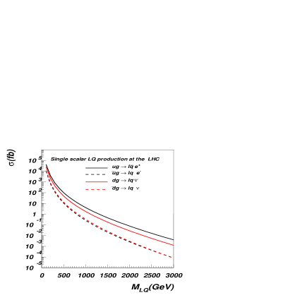
Figure 4: Total cross section of scalar ${L\!\!Q}$ ($S_{0}$) production as a function of the ${L\!\!Q}$ mass for ${L\!\!Q}$ pair (left) and single (right) production at the LHC. The cross section of single ${L\!\!Q}$ production depends on the value ${L\!\!Q}-\ell-q$ coupling chosen to be $\sqrt{g_{3L}^{2}+g_{3L}^{2}}=\lambda_{eff}=e$. The single ${L\!\!Q}$ production in association with charged lepton is represented by black curves while its production in association with neutrino is shown by red curves.

In Fig. 4 we present the total cross section of scalar ${L\!\!Q}$ production as a function of ${L\!\!Q}$ mass for ${L\!\!Q}$ pair (left) and single (right) production. One should note, that single ${L\!\!Q}$ and single $\overline{L\!\!Q}$ production rates at the LHC are drastically different since the first of them is initiated by valence quarks while the other one – by sea quarks. Below, we quote the sum of the cross sections for ${L\!\!Q}$ and $\overline{L\!\!Q}$ single production. ${L\!\!Q}$ single production rates also depend on to which quark(s) it couples. In Fig. 4 one can see the difference in rates for single ${L\!\!Q}$ production when it is produced in association with charged lepton (higher rates) and when it is produced in association with a neutrino (lower rates). The apparent origin of this difference lays in the difference between $up-$ and $down-$ quark parton densities, respectively. We do not lose generality when studying just one type of scalar ${L\!\!Q}$, $S0$ here, since the generic cross section of the scalar ${L\!\!Q}$ single production could be expressed as a superposition of two cross sections represented by the red and black curves in Fig. 4 which scales quadratically with the ${L\!\!Q}-l-q$ coupling. The same is also true for the case of vector ${L\!\!Q}$ production which we describe below.

For low ${L\!\!Q}$ masses ($\sim 100$ GeV) ${L\!\!Q}$ pair production process dominates over the ${L\!\!Q}$ single production process by about one order of magnitude: $\sim 1000$ pb compared with $\sim 100$ pb. But for larger ${L\!\!Q}$ masses ($\sim 1000$ GeV), targeted by LHC (unless Tevatron will discover light ${L\!\!Q}$ states earlier) the cross sections of ${L\!\!Q}$ single and pair production become comparable. This happens because of a stronger phase space suppression of ${L\!\!Q}$ pair production and a related faster drop of the parton (especially gluon) density functions. For $M_{{L\!\!Q}}\sim 1000$ GeV, the cross section for both, single and ${L\!\!Q}$ pair production, is roughly of the order of $10$ fb. For even higher scalar ${L\!\!Q}$ masses, single production starts to dominate over ${L\!\!Q}$ pair production – for $M_{{L\!\!Q}}\sim 2000$ GeV, the ${L\!\!Q}$ single production cross section ($\sim 0.1$ fb) is already one order of magnitude larger than the cross section of pair ${L\!\!Q}$ production ($\sim 0.01$ fb)! Of course, the cross section of ${L\!\!Q}$ single production is proportional to the square of the ${L\!\!Q}-e-q$ unknown coupling (chosen to be equal to the electromagnetic coupling) and can be rescaled accordingly. One can see that if this coupling is of the order of the electromagnetic coupling (like in the case of recent experimental limits obtained at HERA [3]), then the scalar ${L\!\!Q}$ single production should be definitely taken into account and combined with the studies of the ${L\!\!Q}$ pair production.

Figure 5: Total cross section for pair vector ${L\!\!Q}$ production as a function of the ${L\!\!Q}$ mass. Four choices of ($\kappa,\lambda$) are presented: 1) $\kappa_{G}=\lambda_{G}=0$ – Yang-Mills type coupling (YM); 2) $\kappa_{G}=1$, $\lambda_{G}=0$ – Minimal coupling (MC); 3) $\kappa_{G}=-1$, $\lambda_{G}=-1$ – (MM) and 4) the case of absolute minimal cross section (AM) in which the cross-section is minimized with respect to $\kappa_{G},\lambda_{G}$ parameters for each value of $M_{L\!\!Q}$.

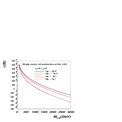
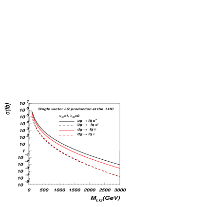
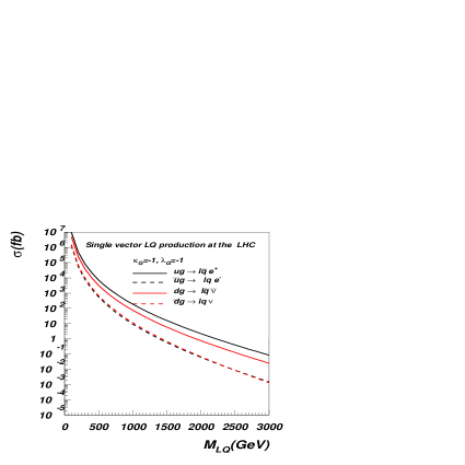
Figure 6: Total cross section of single vector ${L\!\!Q}$($V\!M$) production as a function of the ${L\!\!Q}$ mass. The cross section of ${L\!\!Q}$ single production depends on its quark content and the value ${L\!\!Q}-\ell-q$ coupling chosen to be $\sqrt{g_{2R}^{2}+g_{2L}^{2}}=\lambda_{eff}=e$. single ${L\!\!Q}$ production in association with the charged lepton is denoted by black curves, while its production in association with neutrino is denoted by red curves. Four choices of ($\kappa,\lambda$) are presented: 1) $\kappa_{G}=\lambda_{G}=0$ – Yang-Mills type coupling (YM); 2) $\kappa_{G}=1$, $\lambda_{G}=0$ – Minimal coupling (MC); 3) $\kappa_{G}=-1$, $\lambda_{G}=-1$ – (MM) case and 4) the case of absolute minimal cross section (AM) in which the cross section is minimized with respect to $\kappa_{G},\lambda_{G}$ parameters for each value of $M_{L\!\!Q}$.

Vector ${L\!\!Q}$ cross sections are presented in Fig. 5 and Fig. 6 for the cases of ${L\!\!Q}$ single and pair production, respectively. We present results for four ‘traditional’ choices of $\kappa_{G}$ and $\lambda_{G}$:
1. $\kappa_{G}=\lambda_{G}=0$, Yang-Mills type coupling (YM) case
2. $\kappa_{G}=1$, $\lambda_{G}=0$, Minimal coupling (MC) case
3. $\kappa_{G}=-1$, $\lambda_{G}=-1$, MM case
4. the case of absolute minimal cross section (AM) in which the cross section is minimized with respect to $\kappa_{G},\lambda_{G}$ parameters for each value of $M_{L\!\!Q}$.
For AM case, one can establish the absolute conservative limit on the cross section of vector ${L\!\!Q}$ since for each value of $M_{L\!\!Q}$ the minimal cross section is defined. One can see again, that the cross section for ${L\!\!Q}$ single production catches up the cross section of pair production at $M_{L\!\!Q}\simeq 1$ TeV and starts to dominate at larger ${L\!\!Q}$ masses for the same reason as in scalar ${L\!\!Q}$ production case. One can also notice that the cross section for MC and AM cases are quite close to each other for ${L\!\!Q}$ masses $\leq$ 1 TeV, e.g.at $M_{L\!\!Q}=1.0$ TeV they are 37.6 fb (MC) and 24.8f b (AM) for pair vector ${L\!\!Q}$ production and 31.4 fb (MC) and 30.2 fb (AM) for vector ${L\!\!Q}$ single production. Here, we present the sum of the cross sections, $pp\rightarrow{L\!\!Q}\ell$ and $pp\rightarrow{L\!\!Q}\nu$, of ${L\!\!Q}$ single production processes. However, at higher ${L\!\!Q}$ masses (1.5-2 TeV) the cross section for ${L\!\!Q}$ pair production in the AM case could be a factor of 2-3 smaller than for MC case. This happens because the contribution from $gg\rightarrow{L\!\!Q}\overline{{L\!\!Q}}$ to the total production cross section (which is similar for MC and AM cases) vanishes for heavy ${L\!\!Q}$ production, while the contribution from $q\bar{q}\rightarrow{L\!\!Q}\overline{{L\!\!Q}}$ starts to dominate (it is several times larger for MC, as compared to AM case) in this mass region.

	${L\!\!Q}$ pair production
$M_{L\!\!Q}$	Scalar	Vector ($\kappa,\lambda)$
(TeV)		MM	YM	MC	AM	($\kappa,\lambda$)
		$(-1,-1)$	$(0,0)$	$(1,0)$
0.1	1.04E+06	5.05E+11	8.55E+07	3.34E+07	2.31E+07	(0.549, 0.00363)
0.5	3.45E+02	5.23E+05	2.02E+04	4.12E+03	3.31E+03	(1.01, 0.0496)
1.0	4.20E+00	1.76E+03	2.08E+02	3.76E+01	2.48E+01	(1.16, 0.130)
1.5	1.79E-01	4.89E+01	7.84E+00	1.44E+00	7.12E-01	(1.25, 0.198)
2.0	1.19E-02	2.57E+00	4.70E-01	8.96E-02	3.32E-02	(1.30, 0.239)
	${L\!\!Q}$ single production: $pp(ug)\rightarrow{L\!\!Q}\ell$
$M_{L\!\!Q}$	Scalar	Vector ($\kappa,\lambda)$
(TeV)		MM	YM	MC	AM	($\kappa,\lambda$)
		$(-1,-1)$	$(0,0)$	$(1,0)$
0.1	5.35E+04	1.12E+07	1.87E+06	8.25E+05	8.15E+05	(0.991, 0.0381)
0.5	1.12E+02	7.80E+03	2.22E+03	8.35E+02	8.20E+02	(1.06, 0.0792)
1.0	4.37E+00	1.97E+02	6.05E+01	2.21E+01	2.10E+01	(1.06, 0.0656)
1.5	4.79E-01	1.66E+01	5.15E+00	1.75E+00	1.74E+00	(1.05, 0.0215)
2.0	1.60E-01	2.29E+00	7.10E-01	2.38E-01	2.37E-01	(1.04, -0.0437)
	${L\!\!Q}$ single production: $pp(dg)\rightarrow{L\!\!Q}\nu$
$M_{L\!\!Q}$	Scalar	Vector ($\kappa,\lambda)$
(TeV)		MM	YM	MC	AM	($\kappa,\lambda$)
		$(-1,-1)$	$(0,0)$	$(1,0)$
0.1	3.71E+04	6.55E+06	1.21E+06	5.20E+05	5.15E+05	(1.01, 0.0431)
0.5	6.30E+01	3.93E+03	1.14E+03	4.23E+02	4.15E+02	(1.06, 0.0790)
1.0	2.11E+00	8.70E+01	2.68E+01	9.30E+00	9.20E+00	(1.06, 0.0554)
1.5	2.06E-01	6.60E+00	2.05E+00	6.90E-01	6.90E-01	(1.05, 0.0429)
2.0	3.13E-02	8.25E-01	2.56E-01	8.60E-02	8.55E-02	(1.04, -0.0828)

Table 3: Cross sections (in fb) for ${L\!\!Q}$ single and pair production for vector ($V\!M$) and scalar ($S0$) leptoquarks at the LHC. The cross section of ${L\!\!Q}$ single production depends on its quark content and the value of ${L\!\!Q}-\ell-q$ coupling chosen to be $\sqrt{g_{2R}^{2}+g_{2L}^{2}}=\lambda_{eff}=e$. single ${L\!\!Q}$ production in association with a neutrino is presented separately from ${L\!\!Q}$ production in association with a charged lepton. Four choices for ($\kappa,\lambda$) are presented for vector ${L\!\!Q}$ production: 1) $\kappa_{G}=\lambda_{G}=0$ – Yang-Mills type coupling (YM); 2) $\kappa_{G}=1$, $\lambda_{G}=0$ – Minimal coupling (MC); 3) $\kappa_{G}=-1$, $\lambda_{G}=-1$ – (MM) case and 4) the case of absolute minimal cross section (AM) in which the cross section is minimized with respect to $\kappa_{G},\lambda_{G}$ parameters for each value of $M_{L\!\!Q}$.

The cross section for YM case is typically a factor of 3-5 higher than the one for MC case. For example, for $M_{L\!\!Q}=1.0$ TeV one has 208 fb and 87.3 fb for ${L\!\!Q}$ single and pair production cross section for YM case. For MM case, the cross section for pair ${L\!\!Q}$s is 1-3 orders of magnitude higher than the one for MC case: $\sigma_{L\!\!Q}^{pair}(MM)=1760$ fb for $M_{L\!\!Q}=1.0$ TeV. The MM cross section for ${L\!\!Q}$ single production is about one order of magnitude higher, as compared to MC case: : $\sigma_{L\!\!Q}^{single}(MM)=284$ fb for $M_{L\!\!Q}=1.0$ TeV.

In Table 3, we summarize cross sections for ${L\!\!Q}$ single and pair production for both, vector ($V\!M$) and scalar ($S0$) leptoquarks at the LHC. As we mentioned above, the total cross section for any ${L\!\!Q}$ type can be obtained from Table 3 by superimposing respective numbers and rescaling them for a chosen value of ${L\!\!Q}-\ell-q$ coupling.

In our study we use the MC set of cross sections (which is not very different from AM case) to establish a conservative limit on the $M_{L\!\!Q}$ and $\lambda_{eff}$ parameters of the model.

4 Simulations and signal versus background analysis

The simulations of leptoquark signal events were performed with CompHEP [20], the CompHEP-PYTHIA interface [22] and PYTHIA6.2 [23] program chain. The cross section values presented in this article were calculated using CTEQ6L parton distribution function (PDF)[24]. PYTHIA was used to account for initial and final state radiation and to perform hadronization and decay of resonances, when it was relevant.

Figure 7: Distributions of the cosine of the open angle between electron and jet in events with a scalar (solid line) and vector (dashed line) ${L\!\!Q}$ single production.

Besides the difference in cross section for vector and scalar ${L\!\!Q}$ production one could expect a difference in angular correlations of vector ${L\!\!Q}$ decay products compared to scalar ${L\!\!Q}$ if the vector ${L\!\!Q}$ is being produced with some polarization. We have found that, indeed, vector ${L\!\!Q}$ is produced with non-trivial polarization at the LHC which is reflected, for instance, in a difference in the angular distribution between the leading $p_{T}$ electron and jet shown as an example in Fig. 7 for ${L\!\!Q}$ single production case. The study of such angular correlation effects is, however, beyond the scope of the present article. The distributions of kinematical characteristics we have chosen in this study are similar for scalar and vector ${L\!\!Q}$ production.

The ATLFAST[25] code has been used to take into account the experimental conditions prevailing at LHC for the ATLAS detector. The detector concept and its physics potential have been presented in the Technical Proposal[26] and the Technical Design Report[27]. The ATLFAST code for fast detector simulations accounts for most of the detector features: jet reconstruction in the calorimeters, momentum/energy smearing for leptons and photons, magnetic field effects and missing transverse energy. It provides a list of reconstructed jets, isolated leptons and photons. In most cases, the detector–dependent parameters were tuned to values expected for the performance of the ATLAS detector from full simulation.

The electromagnetic calorimeters were used to reconstruct the energy of leptons in cells of dimensions $\Delta\eta\times\Delta\phi=0.025\times 0.025$ within the pseudorapidity ($\eta$) range $-2.5<\eta<2.5$; $\phi$ is the azimuthal angle. The electromagnetic energy resolution is given by $0.1/\sqrt{E}(GeV)\bigoplus 0.007$ over this pseudorapidity region. The electromagnetic showers are identified as leptons when they lie within a cone of radius $\Delta R=\sqrt{(\Delta\eta)^{2}\times(\Delta\phi)^{2}}=0.2$ and possess a transverse energy $E_{T}>5$ GeV. Lepton isolation criteria were applied, requiring a distance $\Delta R>0.4$ from other clusters and maximum transverse energy deposition, $E_{T}<10$ GeV, in cells in a cone of radius $\Delta R=0.2$ around the direction of electron emission.

Jet energies were reconstructed by clustering hadronic calorimeters cells of dimensions $\Delta\eta\times\Delta\phi=0.1\times 0.1$ within the pseudorapidity range $-2.5<\eta<2.5$. The hadronic energy resolution of the ATLAS detector is parametrized as $0.5/\sqrt{E(GeV)}{\oplus}0.03$ over this $\eta$ region. Hadronic showers are regarded as jets if the deposited transverse energy $E_{T}$ is greater than 15 GeV within a cone of radius $\Delta R=0.4$.

It must be mentioned that standard parametrization in ATLFAST has been used for the electron resolution but detailed studies are needed, using test beam data and GEANT full simulation to validate the extrapolation of the resolution function to electron energies in the TeV range.

In this paper, two types of signal event have been studied.

1. Type 1($2l+jets$) signature, for which ${L\!\!Q}$ produced singly in association with an electron, decays to an electron and a quark, while each ${L\!\!Q}$ produced in pair is required to decay to an electron and a quark.

2. Type 2($l+jets+E_{T}^{miss}$) signature, for which ${L\!\!Q}$ produced singly in association with a neutrino, decays to an electron and a quark.  For ${L\!\!Q}$ pair production, one ${L\!\!Q}$ is required to decay into electron and quark, while the other one – to a neutrino and a quark.

Backgrounds of Type 1 signal signature are $Z+jets$ events, where $Z$ decays into two electrons, and $t\overline{t}$ events where both $W$ from the top quark decay into an electron (positron) and a neutrino. For the signal events of Type 2, backgrounds are $W+jets$ events, where $W$ decays into an electron and a neutrino, and $t\overline{t}$ events where one $W$ decays into an electron and neutrino, and the second $W$ decays into jets.

Table 4: Cross section $\sigma$(pb) from PYTHIA for the backgrounds after pre-selection cuts.

Process	$t\overline{t}$(Type 1)	$t\overline{t}$ (Type 2)	$Z+jet$	$W+jets$
$\sigma$ (pb)	6.6	11	665	17.

In order to enrich the event statistics in the region of high invariant masses, simulated background events were pre-selected in PYTHIA for hard $2\rightarrow 2$ process with transverse momentum, $\hat{p}_{T}>200$ GeV (100 GeV for $Z+jet$ events), defined in the rest frame of the hard interaction, followed by the standard initial and final state radiation technique. Top quark pair production and $W+jets$ background events for Type 2 signal events were additionally pre-selected with at least one electron and $\not\!\!{E_{T}}>100$ GeV. Corresponding cross sections for the backgrounds, used for this article, are shown in Table  4 for the events, passing pre-selection cuts. Since the signal events would consist of events originated from the single or pair production of leptoquarks, we tried to define a unique set of cuts effective for the background suppression against combined ${L\!\!Q}$ pair+single signal.

4.1 Type 1 ${L\!\!Q}$ signal events

Here, we present the analysis of ${L\!\!Q}$ events of Type 1. The signal signatures consist of at least one jet and two electrons.

Due to their large mass, leptoquarks would produce events with large transverse energy. The scalar sum of transverse momenta of all charged particles in the event, $H_{T}$, is presented for single, Fig. 8(left), and pair, Fig. 8(right), scalar ${L\!\!Q}$ production. As can be seen, an appropriate choice of a $H_{T}$ value should suppress the bulk of background events.

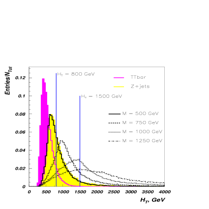
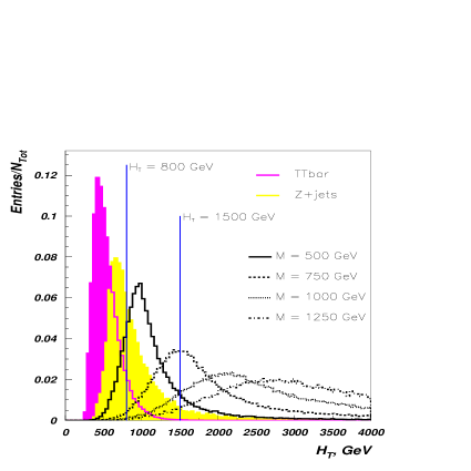
Figure 8: Distribution of the $H_{T}$ variable (see text) for events of single (left) and pair (right) production of scalar leptoquarks and corresponding backgrounds. All distributions are normalized to unity.

The following cuts were used to separate signal from background:

• The transverse momentum of two electrons were required to be at least 90 GeV (100 GeV in the case of $M_{L\!\!Q}>750$ GeV).

• At least one jet was required with minimum transverse momenta of 70 GeV (90 GeV in the case of $M_{L\!\!Q}=750$ GeV and $>100$ GeV/c for higher ${L\!\!Q}$ masses).

• The invariant mass of two electrons was required to be larger than 150 GeV in order to veto the dominant $Z+jets$ background.

• Events with at least one b-jet were vetoed to suppress $t\overline{t}$ background.

• The scalar transverse momentum sum of all selected particles in the event, $H_{T}$, was required to be at least 800 GeV.

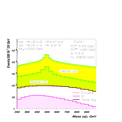
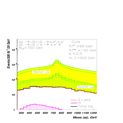
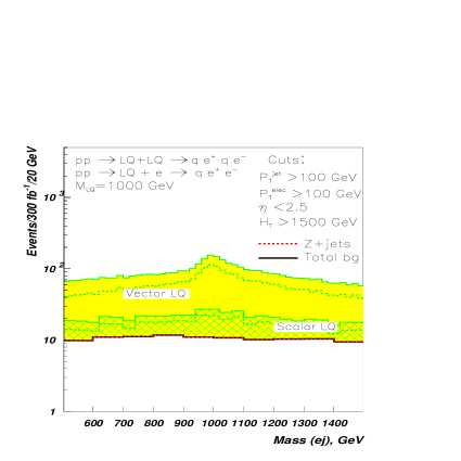
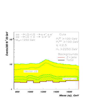
Figure 9: Invariant mass distribution of electron and jet for events of single and pair production of scalar and vector leptoquarks mass $500,750,1000$ and $1250$ GeV for Type 1 signal events.

The resulting invariant mass distributions for the electron-jet system are presented in Figs. 9 for combined single and pair production of leptoquarks of various masses. Signal distributions are presented for scalar (hatched area) and vector leptoquarks. The dashed line shows the pair production contribution to the total signal spectrum. The contribution of the single production to the total spectrum gradually increases with the ${L\!\!Q}$ mass. The cross section for vector leptoquarks corresponds to MC case ($\kappa_{G}=1,\lambda_{G}=0$).

All possible mass combinations between two leading $p_{T}$ jets and electrons are allowed, which leads to some broadening of the signal distributions for the single production case.

As can be seen from these figures, the $Z+jets$ background is essentially dominant. The pair production of top quarks gives a rather small contribution and can be seen only for the lowest leptoquark mass case studied.

The signal statistical significances are given in Table  5. The data are presented for combined (single+${L\!\!Q}$ pair production) signal efficiencies, with the number of events shown for the total background and for ${L\!\!Q}$ single and pair production for different masses of scalar and vector leptoquarks. The data are presented for an integrated luminosity of $L=300fb^{-1}$.

${L\!\!Q}$ Mass	Background	Scalar ${L\!\!Q}$			Vector ${L\!\!Q}$
(GeV)		${L\!\!Q}$-Single	${L\!\!Q}$-Pair	$S_{tot}/\sqrt{B}$	${L\!\!Q}$-Single	${L\!\!Q}$-Pair	$S_{tot}/\sqrt{B}$
500	614	1835	14529	660	25907	155374	7316
750	264	335	1033	84	2902	8571	706
1000	132	54	112	14	392	894	112
1250	40	12	17	5	70	140	33
1500	28	4	3	1	16	20	7

Table 5: Number of signal events for ${L\!\!Q}$ single and pair production versus total background and respective significance $S_{tot}/\sqrt{B}$ for combined signal (${L\!\!Q}$ pair + single production). Results are for an integrated luminosity of $L=300fb^{-1}$ and Type 1 signal signature.

4.2 Type 2 ${L\!\!Q}$ signal events

In this section we present the analysis of signal events with an electron, jets and a neutrino. The signal signature is at least one jet, electron and missing transverse momenta. The scalar sum of transverse momenta of all charged particles in the event, $H_{T}$, is presented for single, Fig. 10 (left), and pair production, Fig. 10 (right) of scalar ${L\!\!Q}$. As can be seen, an appropriate choice of a $H_{T}$ value again should suppress the bulk of background events. The presence of a neutrino in the ${L\!\!Q}$ signal events of this type, provides a possibility to suppress relevant backgrounds using a missing transverse momentum variable. In Fig. 11 (right), we plot the orbital ($\phi$)-angle difference, $\Delta\phi$, between electron and the missing transverse momentum vector. Distributions are shown for scalar and vector leptoquark decays and corresponding backgrounds. The background spectra reveal the emission of an electron and a neutrino along the same direction, which is reasonable, since in background events those particles are produced in $W$ decays. The signal distributions bear mostly the back-to-back emission feature.

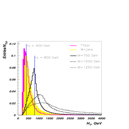
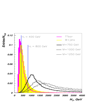
Figure 10: Distribution of $H_{T}$ variable (see text) for events of single (left) and pair (right) production of leptoquarks and corresponding backgrounds. Decays of ${L\!\!Q}$ include electrons and neutrino. All distributions are normalized to unity.

The following set of cuts was worked out to effectively separate the signal from background:

• The transverse momentum of the electron was required to be at least 100 GeV.

• At least one jet was required with a minimum transverse momentum of at least 100 GeV.

• The transverse mass of an electron and the missing transverse momentum vector ($P_{T}^{miss}$, see Fig. 12) was required to be larger than 200 GeV in order to veto the dominant $W+jets$ background.

• Events with at least one b-jet were vetoed to suppress $t\overline{t}$ background.

• The scalar sum of transverse momenta of all selected particles in the event, $H_{T}$, was required to be at least 400,(600, 800, 1000, 1200) GeV for ${L\!\!Q}$ masses of 500, (750, 1000, 1250, 1500) GeV, respectively.

• The orbital angle difference between an electron and the transverse missing momentum vector was required to be greater than 0.8 radians.

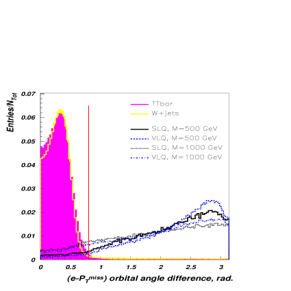
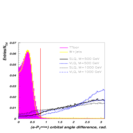
Figure 11: The distribution of the orbital $\phi$-angle difference between an electron and the missing transverse momentum vector, $\Delta\phi$, in radians, for signal (scalar and vector ${L\!\!Q}$) and background $W+jets$ and $t\overline{t}$ events. single (left) and pair (right) ${L\!\!Q}$ production are presented.

While the angular spectra of scalar and vector ${L\!\!Q}$ of $500$ GeV mass are quite close to the background spectra in the forward hemisphere, the signal distributions for larger masses allow the separation of the signal from the background. The resulting invariant mass distributions for the electron-jet system of the signal events of Type 2 are presented in Fig. 13 for the ${L\!\!Q}$ mass of 500 GeV (left side) and 750 GeV (right side). Signal distributions are presented for scalar leptoquarks (hatched area) and vector leptoquarks for the minimal coupling set. The dashed line shows the pair production contribution to the total signal spectrum. Similarly to the Type 1 signal events, the contribution of the single production to the total spectrum gradually increases with the ${L\!\!Q}$ mass. The signal statistical significances are reported in Table  6 combined for ${L\!\!Q}$ single and pair production for different ${L\!\!Q}$ masses. Table  6 also presents number of events, separately for for ${L\!\!Q}$ single and pair production as well as for background events. The data correspond to an integrated luminosity of $L=300fb^{-1}$.

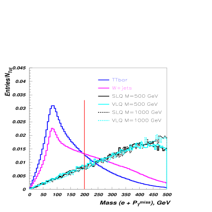
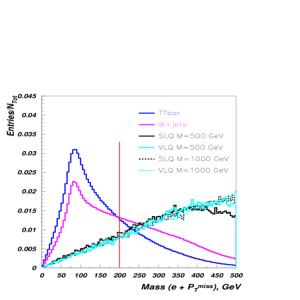
Figure 12: The distribution of the transverse mass of an electron and the $P_{T}^{miss}$ vector for signal (scalar and vector ${L\!\!Q}$) and $W+jets$ and $t\overline{t}$ backgrounds. single (left) and pair (right) ${L\!\!Q}$ production are presented.

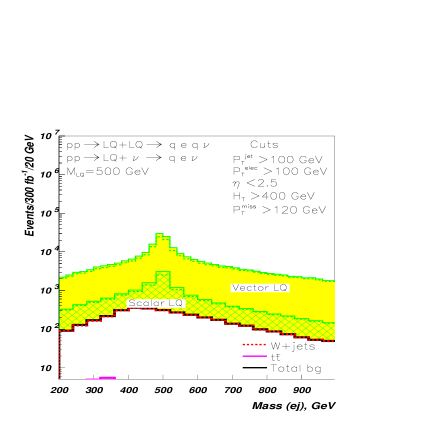
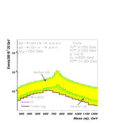
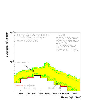
Figure 13: Invariant mass distribution of electron and jet for events of single and pair production of scalar and vector leptoquarks for $m=500$ GeV (upper left) and $m=750$ GeV (upper right) and $m=1000$ GeV (below) for Type 2 signature.

Mass	Background	Scalar ${L\!\!Q}$			Vector ${L\!\!Q}$
(GeV)		${L\!\!Q}$-Single	${L\!\!Q}$-Pair	$S_{tot}/\sqrt{B}$	${L\!\!Q}$-Single	${L\!\!Q}$-Pair	$S_{tot}/\sqrt{B}$
500	1850	2093	8383	244	17889	88438	2425
750	674	251	545	31	1229	4953	238
1000	303	33	52	5	135	460	34
1250	149	5	7	1	17	64	7

Table 6: Number of signal events for single and ${L\!\!Q}$ pair production versus total background and respective significance $S_{tot}/\sqrt{B}$ for combined signal (pair + ${L\!\!Q}$ single production). Results are for an integrated luminosity of $L=300fb^{-1}$ and Type 2 signature.

4.3 ${L\!\!Q}$ mass reach of LHC

The ${L\!\!Q}$ mass reach of LHC is shown in Fig. 14 for combined single and ${L\!\!Q}$ pair production processes and two types of signal signatures. The results for scalar and vector ${L\!\!Q}$ are presented separately. The data are presented for an integrated luminosity of $L=300fb^{-1}$. One can see that scalar leptoquarks can be accessible at LHC up to masses $\lesssim 1.2$ TeV while vector ${L\!\!Q}$ for MC case can be discovered for masses $\lesssim 1.5$ TeV. LHC can exclude ${L\!\!Q}$ at $95\%$ CL with masses about 200 GeV above $5\sigma$ discovery ${L\!\!Q}$ limit, i.e. with masses $\lesssim 1.4$ TeV and $\lesssim 1.7$ TeV for scalar and vector (MC) ${L\!\!Q}$, respectively.

Let us remind, that we have chosen ${L\!\!Q}-l-q$ coupling $\lambda_{eff}=e$ and contribution from ${L\!\!Q}$ single production rescales quadratically with this coupling. For other values of $\lambda_{eff}$, the new LHC reach can be easily found by using LHC reach Tables 5 and 6. One can see that Type 1 signature ($2\ell+jets$) looks more promising compared to Type 2 events ($2\ell+jets+\not\!\!{E_{T}}$).

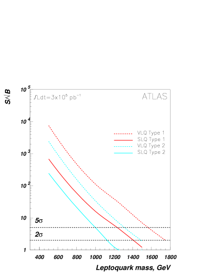
Figure 14: Leptoquark mass reach of the LHC at $5\sigma$ level for Type 1 and Type 2 signal signatures for scalar (solid line) and vector (dashed line) ${L\!\!Q}$ for an integrated luminosity of $L=300fb^{-1}$. For vector ${L\!\!Q}$, the MC choice has been selected. The contributions of single and pair ${L\!\!Q}$ signal are combined.

One should notice that, for the chosen $\lambda_{eff}$, the contribution from ${L\!\!Q}$ single production is 30-50% to the total number of signal events for the ${L\!\!Q}$ mass at the discovery limit. Therefore, ${L\!\!Q}$ single and pair production should be studied together at the LHC . The complementarity of single and pair ${L\!\!Q}$ channels is clearly illustrated in our final Fig. 14, where we present scalar and vector leptoquark mass reach of the LHC in the ($M_{L\!\!Q}-\lambda_{eff}$) plane. For example, for $\lambda_{eff}=1$, ${L\!\!Q}$ single production allows the extension of LHC reach for $M_{L\!\!Q}$ by about 400 GeV!

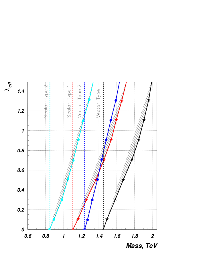
Figure 15: Scalar and vector leptoquark mass reach of the LHC for ($M_{L\!\!Q}--\lambda$) plane for ${L\!\!Q}$ pair production (dashed line) and for combined ${L\!\!Q}$ single and pair production (solid line). Type 1 signal reach contour is denoted by stars while Type 2 signal reach contour is marked by solid dots.

5 Conclusions

In this paper, we present a new detailed study of ${L\!\!Q}$ production and decay at LHC at the level of detector simulation.

We treated ${L\!\!Q}$ single and pair production together and have worked out a set of kinematical cuts to maximize significance for combined single and pair production events.

It was shown, that combination of signatures from ${L\!\!Q}$ single and pair production not only significantly increases the LHC reach, but also allows us to give the correct signal interpretation. Our results are summarized in Tables 5 and 6 and Figs. 14 and 15. In particular, the LHC can discover ${L\!\!Q}$ with a mass up to $1.2$ TeV and $1.5$ TeV for the case of scalar and vector ${L\!\!Q}$, respectively (for $\lambda_{eff}=e$), and ${L\!\!Q}$ single production contributes 30-50% to the total signal rate.

In this work, the most general form of scalar and vector ${L\!\!Q}$ interactions with quarks and gluons has been implemented into CalcHEP/CompHEP packages, which was one of the primary aspects of this study.

References

- [1] For reviews and references see e.g. S. Dimopoulos, S. A. Raby and F. Wilczek, Phys. Today 44N10, 25 (1991); S. Raby in K. Hagiwara et al. [Particle Data Group Collaboration], Phys. Rev. D 66, 010001 (2002).
- [2] B. Schrempp and F. Schrempp, Phys. Lett. B 153, 101 (1985).
- [3] S. Chekanov et al. [ZEUS Collaboration], Phys. Rev. D 68, 052004 (2003) [arXiv:hep-ex/0304008]; C. Adloff et al. [H1 Collaboration], Phys. Lett. B 523, 234 (2001) [arXiv:hep-ex/0107038]; C. Adloff et al. [H1 Collaboration], Phys. Lett. B 479, 358 (2000) [arXiv:hep-ex/0003002]; U. F. Katz [H1 Collaboration], arXiv:hep-ex/9910012; C. Adloff et al. [H1 Collaboration], Eur. Phys. J. C 11, 447 (1999) [Erratum-ibid. C 14, 553 (2000)] [arXiv:hep-ex/9907002].
- [4] V. M. Abazov et al. [D0 Collaboration], Phys. Rev. Lett. 88, 191801 (2002) [arXiv:hep-ex/0111047]; V. M. Abazov et al. [D0 Collaboration], Phys. Rev. D 64, 092004 (2001) [arXiv:hep-ex/0105072]; R. Haas [CDF Collaboration], Int. J. Mod. Phys. A 16S1B, 876 (2001) [arXiv:hep-ex/0010064]; F. Abe et al. [CDF Collaboration], Phys. Rev. Lett. 82, 3206 (1999); F. Abe et al. [CDF Collaboration], Phys. Rev. Lett. 79, 4327 (1997) [arXiv:hep-ex/9708017].
- [5] B. Dion, L. Marleau, G. Simon and M. de Montigny, Eur. Phys. J. C 2, 497 (1998) [arXiv:hep-ph/9701285].
- [6] O. J. P. Eboli, R. Zukanovich Funchal and T. L. Lungov, Phys. Rev. D 57, 1715 (1998) [arXiv:hep-ph/9709319].
- [7] J. E. Cieza Montalvo, O. J. P. Eboli, M. B. Magro and P. G. Mercadante, Phys. Rev. D 58, 095001 (1998) [arXiv:hep-ph/9805472].
- [8] A. Belyaev, O. J. P. Eboli, R. Zukanovich Funchal and T. L. Lungov, Phys. Rev. D 59, 075007 (1999) [arXiv:hep-ph/9811254].
- [9] S. Abdullin and F. Charles, Phys. Lett. B 464, 223 (1999) [arXiv:hep-ph/9905396].
- [10] M. Kramer, T. Plehn, M. Spira and P. M. Zerwas, Phys. Rev. Lett. 79, 341 (1997) [arXiv:hep-ph/9704322].
- [11] M. Kramer, T. Plehn, M. Spira and P. M. Zerwas, arXiv:hep-ph/0411038.
- [12] J. L. Hewett and S. Pakvasa, Phys. Rev. D 37, 3165 (1988).
- [13] O. J. P. Eboli and A. V. Olinto, Phys. Rev. D 38, 3461 (1988).
- [14] B. Dion, L. Marleau and G. Simon, Phys. Rev. D 56, 479 (1997) [arXiv:hep-ph/9610397].
- [15] O. J. P. Eboli and T. L. Lungov, Phys. Rev. D 61, 075015 (2000) [arXiv:hep-ph/9911292].
- [16] W. Buchmuller, R. Ruckl and D. Wyler, Phys. Lett. B 191, 442 (1987) [Erratum-ibid. B 448, 320 (1999)].
- [17] J. Blumlein and R. Ruckl, Phys. Lett. B 304, 337 (1993).
- [18] J. Blumlein, E. Boos and A. Kryukov, Z. Phys. C 76, 137 (1997) [arXiv:hep-ph/9610408].
- [19] P. Cvitanovic, Phys. Rev. D 14, 1536 (1976).
-
[20]
A. Pukhov et al.,
arXiv:hep-ph/9908288;
E. Boos et al. [CompHEP Collaboration], Nucl. Instrum. Meth. A 534, 250 (2004) [arXiv:hep-ph/0403113] - [21] A. Pukhov, arXiv:hep-ph/0412191.
- [22] A. S. Belyaev et al., arXiv:hep-ph/0101232.
- [23] T. Sjostrand, L. Lonnblad and S. Mrenna, arXiv:hep-ph/0108264; T. Sjostrand: Computer Phys. Communications 82 (1994) 74
- [24] J. Pumplin, D. R. Stump, J. Huston, H. L. Lai, P. Nadolsky and W. K. Tung, JHEP 0207, 012 (2002) [arXiv:hep-ph/0201195].
- [25] E. Richter-Was, D. Froidevaux and L. Poggioli: ATLAS Note PHYS-98-131 (1998)
- [26] ATLAS Collaboration, Technical Proposal: Report No. CERN/LHCC/94-43 (1994)
- [27] ATLAS Detector and Physics Performance Technical Design Report. CERN/LHCC/99-14/15, (1999)