Implications for New Physics from Fine-Tuning Arguments: II. Little Higgs Models

Abstract:

We examine the fine-tuning associated to electroweak breaking in Little Higgs scenarios and find it to be always substantial and, generically, much higher than suggested by the rough estimates usually made. This is due to implicit tunings between parameters that can be overlooked at first glance but show up in a more systematic analysis. Focusing on four popular and representative Little Higgs scenarios, we find that the fine-tuning is essentially comparable to that of the Little Hierarchy problem of the Standard Model (that these scenarios attempt to solve) and higher than in supersymmetric models. This does not demonstrate that all Little Higgs models are fine-tuned, but stresses the need of a careful analysis of this issue in model-building before claiming that a particular model is not fine-tuned. In this respect we identify the main sources of potential fine-tuning that should be watched out for, in order to construct a successful Little Higgs model, which seems to be a non-trivial goal.

1 Introduction

In this paper we continue the exam of the implications for new physics from fine-tuning arguments. In a previous paper [1] we revisited the use of the Big Hierarchy problem of the Standard Model (SM) to estimate the scale of new physics, $\Lambda_{\rm SM}$, illustrating our results with two physically relevant examples: right handed (see-saw) neutrinos and supersymmetry (SUSY). Here we study Little Higgs (LH) scenarios as the new physics beyond the SM.

LH models were introduced as an alternative to SUSY in order to solve the Little Hierarchy problem. Very briefly, the latter consists in the following: in the SM (treated as an effective theory valid below $\Lambda_{\rm SM}$) the mass parameter $m^{2}$ in the Higgs potential

$$V={1\over 2}m^{2}h^{2}+{1\over 4}\lambda h^{4}\ ,$$ (1)

receives important quadratically-divergent contributions [2]. At one-loop,

$$\delta_{q}m^{2}={3\over 64\pi^{2}}(3g^{2}+g^{\prime 2}+8\lambda-8\lambda_{t}^{2})\Lambda_{\rm SM}^{2}\ ,$$ (2)

where $g,g^{\prime},\lambda$ and $\lambda_{t}$ are the $SU(2)\times U(1)_{Y}$ gauge couplings, the quartic Higgs coupling and the top Yukawa coupling, respectively. The requirement of no fine-tuning between the above contribution and the tree-level value of $m^{2}$ sets an upper bound on $\Lambda_{\rm SM}$. E.g. for a Higgs mass $m_{h}=115-200$ GeV,

$$\left|{\delta_{q}m^{2}\over m^{2}}\right|\leq 10\ \Rightarrow\ \Lambda_{\rm SM}\stackrel{{\scriptstyle<}}{{{}_{\sim}}}2-3\ {\rm TeV}\ .$$ (3)

This upper bound on $\Lambda_{\rm SM}$ is in a certain tension with the experimental lower bounds on the suppression scale $\Lambda$ of higher order operators, derived from fits to precision electroweak data [3], which typically require $\Lambda\stackrel{{\scriptstyle>}}{{{}_{\sim}}}$ 10 TeV; and this is known as the Little Hierarchy problem.

Let us briefly outline the general structure of LH models. Their two basic ingredients are, first, that the SM Higgs is a Goldstone boson of a spontaneously broken global symmetry; and second, the explicit breaking of this symmetry by gauge and Yukawa couplings in a collective way (a coupling alone is not able to produce enough breaking to give a mass to the SM Higgs). In consequence, the SM Higgs is a pseudo-Goldstone boson, with mass protected at 1-loop from quadratically divergent contributions. In principle, this is enough to avoid the Little Hierarchy problem: if the quadratic corrections to $m^{2}$ appear at the 2-loop level, the extra $(4\pi)^{-2}$ suppression factor in $\delta_{q}m^{2}$ allows for a 10 TeV cut-off with no fine-tuning price.

It should be noticed that the above argument does not imply that in LH models there are no extra states at all below 10 TeV. As discussed in the previous paper [1], even if the quadratic divergences cancel exactly, the new physics states do contribute with logarithmic and finite corrections to $m^{2}$, so their masses should still not be larger than 2–3 TeV (as happens in the supersymmetric case). This is also the case for LH models: the lightest extra states have masses in the TeV range (the scale at which the global symmetry is spontaneously broken), but their contributions to the electroweak observables are calculable and (hopefully) under control. Besides, this effective description is valid up to a cut-off scale, $\Lambda\simeq 10$ TeV, beyond which some unspecified UV completion takes over [4, 5].

Despite the good prospects, the absence of fine-tuning in particular LH scenarios should be checked in practice. More precisely, the fine-tuning must be computed for the different LH models with the same level of rigor employed for the supersymmetric models in the past. A systematic attempt of this kind has not been done up to now, and it is the main goal of this paper. We will focus only on the naturalness of the electroweak breaking, although LH models may have other (model-dependent) problems.

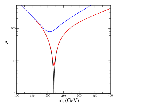
Figure 1: Fine-tuning contours as a function of the Higgs mass in the SM with a cut-off $\Lambda=10$ TeV. This can be considered as the fine-tuning of the Little Hierarchy problem in the SM. Different curves correspond to progressively more sophisticated definitions of $\Delta$ (from black [bottom line] to red to blue [top line], see text for details).

To quantify the fine tuning we follow Barbieri and Giudice [6, 7]: we write the Higgs VEV as $v^{2}=v^{2}(p_{1},p_{2},\cdots)$, where $p_{i}$ are input parameters of the model under study, and define $\Delta_{p_{i}}$, the amount of fine tuning associated to $p_{i}$, by

$${\delta M_{Z}^{2}\over M_{Z}^{2}}={\delta v^{2}\over v^{2}}=\Delta_{p_{i}}{\delta p_{i}\over p_{i}}\ ,$$ (4)

where $\delta M_{Z}^{2}$ (or $\delta v^{2}$) is the change induced in $M_{Z}^{2}$ (or $v^{2}$) by a change $\delta p_{i}$ in $p_{i}$. Roughly speaking, $|\Delta^{-1}_{p_{i}}|$ measures the probability of a cancellation among terms of a given size to obtain a result which is $|\Delta_{p_{i}}|$ times smaller. Due to the statistical meaning of $\Delta_{p_{i}}$, we define the total fine-tuning as

$$\Delta\equiv\left[\sum_{i}\Delta_{p_{i}}^{2}\right]^{1/2}\ .$$ (5)

It is important to recall that the Little Hierarchy problem of the SM, which the LH models attempt to solve, is itself a fine-tuning problem: one could simply assume $\Lambda_{\rm SM}\stackrel{{\scriptstyle>}}{{{}_{\sim}}}10$ TeV with the ’only’ price of tuning $\delta_{q}m^{2}$, as given by eq. (2), at the 0.4–1 % level (or, equivalently, $\Delta=100-250$). Therefore, to be of interest, the LH models should at least improve this degree of fine-tuning. In order to perform a fair comparison, this estimate can be refined following the lines explained in refs. [1, 8, 9]. First of all, eq. (2) should be renormalization-group improved. Then, the value of $\Delta$ $(=\Delta_{\Lambda})$ vs. $m_{h}$ is given by the (bottom) black line of fig. 1. The deep throat at $m_{h}\sim 220$ GeV results from an accidental cancellation between the various terms in eq. (2). This throat is cut when the fine-tuning parameter associated to the top mass ($\Delta_{\lambda_{t}}$) is added in quadrature as explained above (for details see ref. [1]), giving the (middle) red line. Finally, once the fine-tuning parameter associated to the Higgs mass itself ($\Delta_{\lambda}$) is included as well, the value of $\Delta$ is given by the (top) blue line, which thus represents the fine-tuning associated to the Little Hierarchy problem. This has to be compared with the tuning of LH models. On the other hand, for the minimal supersymmetric standard model (MSSM) the degree of fine-tuning is presently at the few percent level ($\Delta\simeq 20-40$ for $m_{h}\stackrel{{\scriptstyle<}}{{{}_{\sim}}}125$ GeV), while for other supersymmetric models the situation is much better [10, 11]. Hence, in order to be competitive with supersymmetry, LH models should not worsen the MSSM performance. We will use these criteria in order to analyze the success of several representative LH models.

Due to the great variety of LH models we do not attempt to perform here an exhaustive analysis of them. Rather, we have focused on four LH scenarios [12, 13, 14, 15] which are probably the most popular ones, and tried to extract general lessons for other models. The prototype LH scenario is the so-called Littlest Higgs model [12]. This model is a very good example to start with, due to its simplicity and because it shares many features with more elaborate LH constructions. Actually, many of those models are simply modifications of the Littlest Higgs model. The Littlest Higgs has some phenomenological problems with the constraints from precision electroweak observables. (Incidentally, this illustrates the fact that the impact of the TeV–mass states of LH models on electroweak observables is not always under control [16].) Since our focus is the naturalness of electroweak breaking, we will ignore those constraints, although the strongest results would come from combining both analyses. On the other hand, there exist modifications of the Littlest Higgs (also studied in this paper) able to overcome those difficulties.

The paper is organized as follows. In sect. 2 we analyze the structure, and evaluate the fine-tuning, of the Littlest Higgs model. Sections 3 and 4 are devoted respectively to the computation of the fine-tuning in two popular modifications of the Littlest Higgs proposed in refs. [13] and [14]. The latter corresponds to the so-called Littlest Higgs model with $T$-parity. In sect. 5 we study a recent proposal (the so-called “Simplest Little Higgs” [15]), whose structure differs substantially from the Littlest Higgs. In all these cases the fine-tuning turns out to be essentially comparable with that of the Little Hierarchy problem of the SM (that LH models attempt to solve) and higher than in supersymmetric models, and we discuss the reasons for this fact. Finally, in sect. 6 we summarize our results and present some conclusions. In addition we present in Appendix A a simple recipe to evaluate the fine-tuning when the various parameters of a model are subject to constraints. Appendix B contains details on the structure of the different Little Higgs models studied.

2 The Littlest Higgs [12]

2.1 Structure of the model

The Littlest Higgs model is a non-linear sigma model based on a global $SU(5)$ symmetry, spontaneously broken to $SO(5)$ at a scale $f\sim 1$ TeV, and explicitly broken by the gauging of an $[SU(2)\times U(1)]^{2}$ subgroup. After the spontaneous breaking, the latter gets broken to its diagonal subgroup, identified with the SM electroweak gauge group, $SU(2)_{L}\times U(1)_{Y}$. From the 14 (pseudo)-Goldstone bosons of the $SU(5)\rightarrow SO(5)$ breaking, 4 degrees of freedom (d.o.f.) are true Goldstones [eaten by the gauge bosons of the spontaneously broken (“axial”) $SU(2)\times U(1)$, which thus acquire masses $\sim f\sim 1$ TeV through the Higgs mechanism] and the remaining 10 d.o.f. correspond to the SM Higgs doublet, $H=(h^{0},h^{+})$, (4 d.o.f.) and a complex $SU(2)_{L}$ scalar triplet, $\phi$ (6 d.o.f.) with $Y=1$; in vectorial notation, $\phi=(\phi^{++},\phi^{+},\phi^{0})$. All these fields can be treated simultaneously in a nonlinear matrix field $\Sigma$ (see Appendix B for details).

The $[SU(2)\times U(1)]^{2}$ gauge interactions give a radiative mass to the SM Higgs, but only when the couplings of both groups are simultaneously present, as explained in more detail below. Hence, the quadratically divergent contributions only appear at two-loop order, and the high-energy cut-off can be pushed up to a scale $\Lambda\sim 4\pi f\sim 10$ TeV, as explained in the introduction. For the potentially dangerous top-Yukawa interactions things work in a similar way: the spectrum is enlarged with two extra fermions of opposite chiralities, and the conventional top-Yukawa coupling, $\lambda_{t}$, is not an input parameter but results from two independent couplings $\lambda_{1},\lambda_{2}$. Both must be present in order to generate a radiative correction to the Higgs mass, and this again forbids quadratically divergent corrections to $m_{h}^{2}$ at one–loop.

For our purposes, the relevant states besides those of the SM are: the pseudo-Goldstone bosons $H,\phi$; the heavy gauge bosons, $W^{\prime},B^{\prime}$, of the axial $SU(2)\times U(1)$; and the two extra (left and right) fermionic d.o.f. that combine in a vector-like “heavy Top”, $T$. The relevant part of the Lagrangian can be found in Appendix B, eqs. (B.8) and (B.10). It consists of two pieces

$${\cal L}={\cal L}_{kin}(g_{1},g_{2},g_{1}^{\prime},g_{2}^{\prime})\ +\ {\cal L}_{f}(\lambda_{1},\lambda_{2})\ ,$$ (6)

where $g_{1},g^{\prime}_{1}$ ($g_{2},g^{\prime}_{2}$) are the gauge couplings of the first (second) $SU(2)\times U(1)$ factor, and $\lambda_{1},\lambda_{2}$ are the two independent fermionic couplings. These couplings are constrained by the relations with the SM couplings,

$${1\over g^{2}}={1\over g_{1}^{2}}+{1\over g_{2}^{2}}\ ,\;\;\;\;\;\ {1\over g^{\prime 2}}={1\over g_{1}^{\prime 2}}+{1\over g_{2}^{\prime 2}}\ ,\;\;\;\;\;{2\over\lambda_{t}^{2}}={1\over\lambda_{1}^{2}}+{1\over\lambda_{2}^{2}}\ ,$$ (7)

where $g$ and $g^{\prime}$ are the $SU(2)$ and $U(1)_{Y}$ gauge couplings, respectively, and $\lambda_{t}$ is the top Yukawa coupling. The Lagrangian (6) gives ${\cal O}(f)$ masses to $W^{\prime},B^{\prime}$ and $T$. These heavy masses have a non-trivial dependence on the full non-linear field $\Sigma$, which contains the $H$ and $\phi$ fields. In particular, retaining only the dependence on $h\simeq{\rm Re}(h^{0})\sqrt{2}$ we get

$$m_{W^{\prime}}^{2}(h) = M_{W^{\prime}}^{2}+{\cal O}(h^{2})={1\over 4}(g_{1}^{2}+g_{2}^{2})f^{2}-{1\over 4}g^{2}h^{2}+{\cal O}(h^{4}/f^{2})\ ,$$

$$m_{B^{\prime}}^{2}(h) = M_{B^{\prime}}^{2}+{\cal O}(h^{2})={1\over 20}(g_{1}^{\prime 2}+g_{2}^{\prime 2})f^{2}-{1\over 4}g^{\prime 2}h^{2}+{\cal O}(h^{4}/f^{2})\ ,$$

$$m_{T}^{2}(h) = M_{T}^{2}+{\cal O}(h^{2})=(\lambda_{1}^{2}+\lambda_{2}^{2})f^{2}-{1\over 2}\lambda_{t}^{2}h^{2}+{\cal O}(h^{4}/f^{2})\ .$$ (8)

At this level, $H$ and $\phi$ are massless, but they get massive radiatively. The simplest way to see this is by using the effective potential. Let us consider first the quadratically divergent contribution to the one-loop scalar potential, given by

$$V_{1}^{\rm quad}={1\over 32\pi^{2}}\Lambda^{2}\ {\rm Str}{\cal M}^{2}\ ,$$ (9)

where the supertrace ${\rm Str}$ counts degrees of freedom with a minus sign for fermions, and ${\cal M}^{2}$ is the (tree-level, field-dependent) mass-squared matrix. In our case, the previous formula gives

$$V_{1}^{\rm quad}={1\over 32\pi^{2}}\Lambda^{2}\ \left[6m_{W}^{2}+9m_{W^{\prime}}^{2}+3m_{Z}^{2}+3m_{B^{\prime}}^{2}-12(m_{t}^{2}+m_{T}^{2})\right]\ .$$ (10)

By looking at the $h$-dependence of the masses above it is easy to check that $V_{1}^{\rm quad}$ does not contain a mass term for $h$ (this will be generated by the logarithmic and finite contributions to the potential, to be discussed shortly). The reason for this result is the following. If $\lambda_{1}=g_{2}=g_{2}^{\prime}=0$, the Lagrangian (6) recovers a global $SU(3)$ [$SU(3)_{1}$, living in the upper corner of $SU(5)$] that protects the mass of the Higgs (which transforms by a shift under that symmetry). On the other hand, if $\lambda_{2}=g_{1}=g_{1}^{\prime}=0$, then a different $SU(3)$ symmetry [$SU(3)_{2}$, living in the lower corner of $SU(5)$] is recovered that also protects the Higgs mass. A non-zero value for the Higgs mass can only be generated by breaking both $SU(3)$’s and therefore both type-1 and type-2 couplings should be present. Quadratically divergent diagrams involve only one type of coupling and therefore cannot contribute to the Higgs mass. This is the so-called collective breaking of the original $SU(5)$ symmetry and is one of the main ingredients of Little Higgs models.

These symmetries do not protect the mass of the triplet. In fact, if we include the full dependence of the bosonic ($W^{\prime},B^{\prime}$) and fermionic ($T$) masses on the $\Sigma$ field, $V_{1}^{\rm quad}$ contains operators, ${\cal O}_{V}(\Sigma)$ and ${\cal O}_{F}(\Sigma)$ respectively, that produce a mass term for the triplet $\phi$ of order $\Lambda^{2}/(16\pi^{2})\sim f^{2}$. Explicit expressions for these operators are given in Appendix B. Then, following [12], it is reasonable to assume that ${\cal O}_{V}(\Sigma)$ and ${\cal O}_{F}(\Sigma)$ are already present at tree-level, as a remnant of the heavy physics integrated out at $\Lambda$ (a threshold effect). These effects can be accounted for by adding an extra piece to the Lagrangian,

$$-\Delta{\cal L}=c\ {\cal O}_{V}(\Sigma)\ +\ c^{\prime}\ {\cal O}_{F}(\Sigma)\ ,$$ (11)

were $c$ and $c^{\prime}$ are unknown coefficients [see eq. (B.11) in Appendix B for an explicit expression of $\Delta{\cal L}$]. For future use, it is convenient to discuss here what is the natural size of $c$ and $c^{\prime}$. Naive dimensional analysis [17] has been used to estimate $c,c^{\prime}\sim{\cal O}(1)$. We can make a more precise evaluation by computing the one-loop contributions to $c$ and $c^{\prime}$ coming from (10), keeping the full dependence of the masses on $\Sigma$. Then we get

$$c = c_{0}\ +\ c_{1}=c_{0}\ +3/4\ ,$$

$$c^{\prime} = c_{0}^{\prime}\ +\ c_{1}^{\prime}=c_{0}^{\prime}\ -{24}\ .$$ (12)

where the subindex 0 labels the unknown threshold contributions from physics beyond $\Lambda$.

Besides giving a mass to $\phi$, the operators in eq. (11) produce a coupling $\sim h^{2}\phi$ and a quartic coupling for $h$. This quartic coupling is modified by the presence of the $h^{2}\phi$ term once the heavy triplet is integrated out. After that is done, the Higgs quartic coupling $\lambda$ can be written in the simplest manner as

$${1\over\lambda}={1\over\lambda_{a}}+{1\over\lambda_{b}}\ ,$$ (13)

with

$$\lambda_{a}\equiv c(g_{2}^{2}+g_{2}^{\prime 2})-c^{\prime}\lambda_{1}^{2}\ ,\;\;\;\;\;\lambda_{b}\equiv c(g_{1}^{2}+g_{1}^{\prime 2})\ .$$ (14)

We see that the structure of (13) is similar to that of (7) for the fermion and gauge boson couplings, with $\lambda_{a}$ ($\lambda_{b}$) being a type-1 (type-2) coupling.

In order to write the one-loop Higgs potential, we need explicit expressions for the $h$-dependent masses of the spectrum. In the scalar sector, we decompose $h^{0}\equiv(h^{0r}+ih^{0i})/\sqrt{2}$ and $\phi^{0}\equiv i(\phi^{0r}+i\phi^{0i})/\sqrt{2}$. In the $CP$-even sector we write the relevant part of the mass matrix in the basis $\{h^{0r},\phi^{0r}\}$; in the $CP$-odd sector we use the basis $\{h^{0i},\phi^{0i}\}$ and finally, in the charged sector the basis $\{h^{+},\phi^{+}\}$. The three mass matrices are very similar in structure and can be written simultaneously as

$$M^{2}_{\kappa}(h)=\left[\begin{array}[]{cc}{1\over 4}a_{\kappa}\lambda_{+}h^{2}+{1\over\sqrt{2}}s_{\kappa}\lambda_{-}ft+{\cal O}(h^{4}/f^{2})&b_{\kappa}\lambda_{-}fh+{\cal O}(h^{2})\\ &\\ b^{*}_{\kappa}\lambda_{-}fh+{\cal O}(h^{2})&\lambda_{+}(f^{2}-c_{\kappa}h^{2})+{\cal O}(h^{4}/f^{2})\end{array}\right]\ ,$$ (15)

where the index $\kappa=\{0r,0i,+\}$ labels the different sectors, $a_{\kappa}=\{3,1,1\}$, $s_{\kappa}=\{1,-1,0\}$, $b_{\kappa}=\{1/\sqrt{2},1/\sqrt{2},i/2\}$, $c_{\kappa}=|b_{\kappa}|^{2}$, and we have defined $\lambda_{+}\equiv\lambda_{a}+\lambda_{b}$, $\lambda_{-}\equiv\lambda_{a}-\lambda_{b}$. We have also included in these mass matrices the contribution of the triplet VEV, $t\equiv\langle\phi^{0r}\rangle$, with

$$t\simeq-{1\over 2\sqrt{2}}{\lambda_{-}h^{2}\over\lambda_{+}f}\ .$$ (16)

The off-diagonal entries in (15) are due to the $h^{2}\phi$ coupling and they cause mixing between $h$ and $\phi$. Concerning the masses, the effect of this mixing is negligible for the triplet [at order $h^{2}$, the masses of $\phi^{0r}$ and $\phi^{0i}$ are the same, and these fields can still be combined in a complex field $\phi^{0}$]. Explicitly, these masses are

$$\left[\begin{array}[]{c}m_{\phi^{0}}^{2}(h)\\ m_{\phi^{+}}^{2}(h)\\ m_{\phi^{++}}^{2}(h)\end{array}\right]=M_{\phi}^{2}+{\cal O}(h^{2})=(\lambda_{a}+\lambda_{b})f^{2}-\left[\begin{array}[]{c}2\\ 1\\ 0\end{array}\right]\lambda h^{2}+{\cal O}(h^{4}/f^{2})\ .$$ (17)

We will call ${h^{\prime}}^{0r}$, ${h^{\prime}}^{0i}$ and ${h^{\prime}}^{+}$ the light mass eigenstates of (15) in the different sectors, for which we get

$$\left[\begin{array}[]{c}m^{2}_{{h^{\prime}}^{0r}}(h)\\ m^{2}_{{h^{\prime}}^{0i}}(h)\\ m^{2}_{{h^{\prime}}^{+}}(h)\end{array}\right]=\left[\begin{array}[]{c}3\\ 1\\ 1\end{array}\right]\lambda h^{2}+{\cal O}(h^{4}/f^{2})\ .$$ (18)

From the previous expressions it is straightforward to check that, in the contribution of scalars to $V_{1}^{\rm quad}$,

$${\Lambda^{2}\over 32\pi^{2}}\left(m_{{h^{\prime}}^{0r}}^{2}+m_{{h^{\prime}}^{0i}}^{2}+2m_{{h^{\prime}}^{+}}^{2}+2m_{\phi^{0}}^{2}+2m_{\phi^{+}}^{2}+2m_{\phi^{++}}^{2}\right)\ ,$$ (19)

there is also a cancellation of $h^{2}$ terms. This is due to the fact that the operators of (11) still respect the same $SU(3)_{i}$ symmetries of the original Lagrangian as they originate from quadratically divergent one–loop corrections.

Finally, a non-vanishing mass parameter for $h$ arises from the logarithmic and finite contributions to the effective potential. In the $\overline{\rm MS}$ scheme, in Landau gauge, and setting the renormalization scale $Q=\Lambda$,

$$m^{2} = {3\over 64\pi^{2}}\left\{3g^{2}M_{W^{\prime}}^{2}\left[\log{\Lambda^{2}\over M_{W^{\prime}}^{2}}+{1\over 3}\right]+g^{\prime 2}M_{B^{\prime}}^{2}\left[\log{\Lambda^{2}\over M_{B^{\prime}}^{2}}+{1\over 3}\right]\right\}$$ (20)

$$+ {3\lambda\over 8\pi^{2}}M_{\phi}^{2}\left[\log{\Lambda^{2}\over M_{\phi}^{2}}+1\right]-{3\lambda_{t}^{2}\over 8\pi^{2}}M_{T}^{2}\left[\log{\Lambda^{2}\over M_{T}^{2}}+1\right]\ ,$$

where we have included the contribution from the $\phi$ masses.

In summary, the effective potential of the Higgs field can be written in the SM-like form

$$V={1\over 2}m^{2}h^{2}+{1\over 4}\lambda h^{4}\ ,$$ (21)

where $\lambda$ and $m^{2}$ are given by eqs. (13) and (20). The Higgs VEV is simply

$$v^{2}=-{m^{2}\over\lambda}\ .$$ (22)

2.2 Fine-tuning analysis

A rough estimate of the fine-tuning associated to electroweak breaking in the Littlest Higgs model can be obtained from eq. (20). The contribution of the heavy Top, $T$, to the Higgs mass parameter is

$$\delta_{T}m^{2}=-{3\lambda_{t}^{2}\over 8\pi^{2}}M_{T}^{2}\left[\log{\Lambda^{2}\over M_{T}^{2}}+1\right]\ .$$ (23)

Using eqs. (7) and (2.1), it follows that $M_{T}^{2}\geq 2\lambda_{t}^{2}f^{2}$, and thus $\delta_{T}m^{2}\geq 0.37f^{2}$ (the minimum corresponds to $\lambda_{1}=\lambda_{2}=\lambda_{t}$). Thus the ratio $\delta_{T}m^{2}/m^{2}$, tends to be quite large: e.g. for $f=1$ TeV and $m_{h}=115,150,250$ GeV, one gets $|\delta_{T}m^{2}/m^{2}|\geq 56,\ 33,\ 12$ respectively. Since there are other potential sources of fine-tuning, this should be considered as a lower bound on the total fine-tuning. Actually, the overall fine tuning is usually much larger than this estimate, as we show below. (Eventually we will go back to this rough argument to improve it in a simple way.)

In order to perform a complete fine-tuning analysis we determine first the input parameters, $p_{i}$, and then calculate the associated fine-tunings, $\Delta_{p_{i}}$, according to eq. (4), i.e. $\Delta_{p_{i}}=(p_{i}/v^{2})(\partial v^{2}/\partial p_{i})$. For the Littlest Higgs model the input parameters of the Lagrangian [eqs. (6) and (11)] are

$$p_{i}\ =\ \{g_{1},\ g_{2},\ g_{1}^{\prime},\ g_{2}^{\prime},\ \lambda_{1},\ \lambda_{2},\ c,\ c^{\prime},\ f\}\ .$$ (24)

We have not included $\Lambda$ among these parameters since we are assuming $\Lambda\simeq 4\pi f$. On the other hand, the parameter $f$ basically appears as a multiplicative factor in the mass parameter, $m^{2}$, so $\Delta_{f}$ is always ${\cal O}(1)$, and can be ignored. Finally, the above parameters are constrained by the measured values of the top mass and the gauge couplings $g,g^{\prime}$, according to eq. (7). The procedure to estimate the fine-tuning in the presence of constraints is discussed in Appendix A. The net effect is a reduction of the “unconstrained” total fine-tuning, $\Delta=(\sum_{i}\Delta_{p_{i}}^{2})^{1/2}$, according to eq. (A.6). In this particular case, that equation gives

$$\Delta=\left[\sum_{i}\Delta_{p_{i}}^{2}-\sum_{\alpha=1}^{3}{1\over N_{\alpha}^{2}}\left(\sum_{i}p_{i}{\partial G^{(0)}_{\alpha}\over\partial p_{i}}\Delta_{p_{i}}\right)^{2}\right]^{1/2}\ ,$$ (25)

where $G^{(0)}_{\alpha}=\{g^{2},g^{\prime 2},\lambda_{t}^{2}\}$ are functions of the $p_{i}$ as given in eq. (7), and

$$N_{\alpha}^{2}\equiv\sum_{i}p_{i}^{2}\left({\partial G^{(0)}_{\alpha}\over\partial p_{i}}\right)^{2}\ ,$$ (26)

are normalization constants.

As announced before, $\Delta$ is in general much larger than the initial rough estimate, although the precise magnitude depends strongly on the region of parameter space considered and decreases significantly as $m_{h}$ increases. Let us discuss how this comes about. The negative contribution from $M_{T}^{2}$ to $m^{2}$ in eq. (20) must be compensated by other positive contributions. Typically, this requires a large value of the triplet mass, $M_{\phi}^{2}=(\lambda_{a}+\lambda_{b})f^{2}$, which requires a large value of $(\lambda_{a}+\lambda_{b})$, but keeping $1/\lambda=1/\lambda_{a}+1/\lambda_{b}$ fixed for a given $m_{h}$. There are two ways of achieving this:

$${\rm a)} \;\;\lambda\simeq\lambda_{b}\ll\lambda_{a}\simeq M_{\phi}^{2}/f^{2}\ ,$$

$${\rm b)} \;\;\lambda\simeq\lambda_{a}\ll\lambda_{b}\simeq M_{\phi}^{2}/f^{2}\ .$$ (27)

Notice that the one-loop $m^{2}$ is a symmetric function of $\lambda_{a}$ and $\lambda_{b}$, so cases ${\rm a)}$ and ${\rm b)}$ are simply related by $\lambda_{a}\leftrightarrow\lambda_{b}$. This means that the triplet and Higgs masses are exactly the same in both cases although the fine-tuning may be different (since the dependence of $\lambda_{a,b}$ on $p_{i}$ is not the same), and indeed it is, as we discuss next.

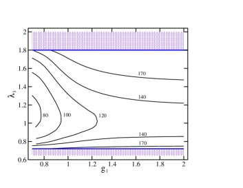
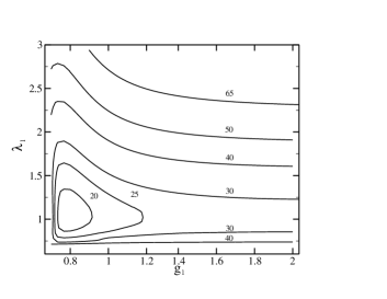
Figure 2: Preliminary fine-tuning contours for the Littlest Higgs model, case a) of eq. (2.2), for two different values of the Higgs mass: $m_{h}=115$ GeV (left) and $m_{h}=250$ GeV (right).

For case a), the value of $\Delta$ is shown by the contour plots of fig. 2 which correspond to two different values of the Higgs mass. We present our results in the plane $\{g_{1},\lambda_{1}\}$. In each point of this plane, $g_{2}$ and $\lambda_{2}$ are then fixed by eq. (7); the values of $c$ and $c^{\prime}$ are fixed by the minimization condition for electroweak breaking and the choice of Higgs mass. The value of $g_{1}^{\prime}$ has been taken at $g_{1}^{\prime 2}=g_{2}^{\prime 2}=g^{\prime 2}/2$, which nearly minimizes the fine-tuning. (Note also that $g_{1}\geq g$ and thus smaller values of $\Delta$ cannot be reached by lowering $g_{1}$ in fig. 2.) The shaded areas correspond to regions that do not give a correct electroweak symmetry breaking (in these regions, $M_{\phi}\geq\Lambda$, which besides being beyond the range of validity of the effective theory, makes negative the triplet contribution to $m^{2}$). These plots illustrate the large size of $\Delta$, which is significantly larger than the previous rough estimate. This is not surprising since, as stated before, besides the heavy top contribution to $m^{2}$ (on which the estimate was based), there are other contributions that depend in various ways on the different input parameters. This gives additional contributions to the total fine-tuning, increasing its value. The plots also show how $\Delta$ decreases for increasing $m_{h}$. This is due to the fact that the larger $m_{h}$, and thus $\lambda$, the larger the required value of $m^{2}$ in (22), which reduces the level of cancellation needed between the various contributions to $m^{2}$ in (20) [1]. Although the fine-tuning is substantial, it could be considered as tolerable [i.e. ${\cal O}(10)$], for some (small) regions of parameter space, at least for large $m_{h}$. However, on closer examination the fine-tuning turns out to be larger than shown by fig. 2. From the condition a) in (2.2)

$$\lambda\simeq c(g_{1}^{2}+g_{1}^{\prime 2})=\lambda_{b}\ll\lambda_{a}=c(g_{2}^{2}+g_{2}^{\prime 2})-c^{\prime}\lambda_{1}^{2}\ ,$$ (28)

it is clear that in this case $c^{\prime}$ is large (and negative), while $c$ is small. But then, eq. (2.1) shows that there is an implicit tuning between $c_{0}$ and $c_{1}$ to get the small value of $c$. In fact, it makes more sense to include $c_{0}$ and $c_{0}^{\prime}$, rather than $c$ and $c^{\prime}$, among the unknown input parameters appearing in (24). Then, since $\Delta_{c_{0}}=|(c_{0}/c)\Delta_{c}|$ (and similarly for $\Delta_{c_{0}^{\prime}}$), the global fine-tuning becomes much larger. This is illustrated in fig. 3 (upper plots), where $\Delta$ is systematically above ${\cal O}(10)$, even for large $m_{h}$.

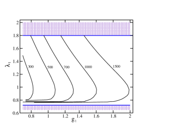
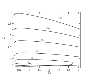
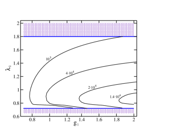
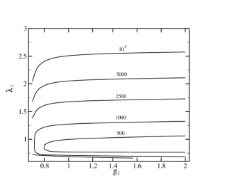
Figure 3: Final fine-tuning contours for the Littlest Higgs model, using $c_{0}$ and $c^{\prime}_{0}$ of eq. (2.1) as unknown parameters to improve the analysis. TOP: Case a) of eq. (2.2) for $m_{h}=115$ GeV (left) and $m_{h}=250$ GeV (right). BOTTOM: The same but for case b) of eq. (2.2).

There is a simple way of understanding the order of magnitude of $\Delta$. We can repeat the rough argument at the beginning of this subsection, but considering now the contribution of the triplet to the Higgs mass parameter in (20). More precisely, since $M_{\phi}^{2}=(\lambda_{a}+\lambda_{b})f^{2}=[c(g_{1}^{2}+g_{1}^{\prime 2}+g_{2}^{2}+g_{2}^{\prime 2})-c^{\prime}\lambda_{1}^{2}]f^{2}$, we can focus on the contribution proportional to $c^{\prime}$:

$$\delta_{c^{\prime}}m^{2}=-{3\lambda\over 8\pi^{2}}c^{\prime}\lambda_{1}^{2}\left[\log{\Lambda^{2}\over M_{\phi}^{2}}+1\right]\ .$$ (29)

Now, $c^{\prime}$ itself contains a radiative piece $c^{\prime}_{1}=-24$ [see eq. (2.1)], whose relative contribution to $m^{2}$ is then given by

$$\left|{\delta_{c^{\prime}_{1}}m^{2}\over m^{2}}\right|\geq{9\over 2\pi^{2}}\lambda_{t}^{2}{f^{2}\over v^{2}}\left[\log{\Lambda^{2}\over M_{\phi}^{2}}+1\right]\ \simeq 45\ ,$$ (30)

where we have first used $\lambda_{1}^{2}\geq\lambda_{t}^{2}/2$ and then $M_{\phi}\sim f$. Hence we easily expect ${\cal O}(100)$ contributions to $\Delta$, as reflected in fig. 3.

It is interesting to note that this rough argument holds even if there are additional contributions to $m^{2}$, since it is based on the size of contributions that are present anyway. In particular, two-loop corrections or ‘tree-level’ (i.e. threshold) corrections to $m^{2}$ are not likely to help in improving the fine-tuning. Of course, it might happen that they have just the right size to cancel the known large contributions, such as those of eqs. (23) and (30). However, in the absence of a theoretical argument for that cancellation, this possibility can only be understood a priori as a fortunate accident. The chances for the latter are precisely what the fine-tuning analysis evaluates.

For case b) in eq. (2.2) things are much worse, as illustrated in fig. 3 (lower plots), which shows huge values of $\Delta$. The reason is the following. In case ${\rm b)}$, both $c$ and $c^{\prime}$ are sizeable, so there is no implicit tuning between $c_{0}$ ($c_{0}^{\prime}$) and $c_{1}$ ($c_{1}^{\prime}$), but this implies a cancellation to get $\lambda_{a}=c(g_{2}^{2}+g_{2}^{\prime 2})-c^{\prime}\lambda_{1}^{2}\simeq\lambda$, which requires a delicate tuning. This “hidden fine-tuning” is responsible for the unexpectedly large values of $\Delta$. In other words, small changes in the input parameters of the model produce large changes in the value of $\lambda$, and thus in the value of $v^{2}$.

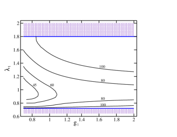
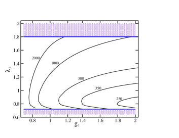
Figure 4: LEFT: The same as the bottom-left plot of fig. 3, but keeping $\lambda$ fixed. RIGHT: Fine-tuning associated to $\lambda$ itself in the same case.

Now, imagine some future time after the Higgs mass has already been measured so that the parameter $\lambda$ takes a particular value and the other parameters of the model can only be varied in such a way that $\lambda$ remains constant. Then, according to the above discussion, the fine-tuning for case b) should be dramatically reduced and, apparently, this is exactly what happens. The condition of constant $\lambda$ can be incorporated in the computation of $\Delta$ using eq. (A.6) with an additional constraint $G_{4}^{(0)}=\lambda$. The new “constrained” fine tuning in case b) (for $m_{h}=115$ GeV), is shown in the left plot of fig. 4, to be compared with the bottom-left plot of fig. 3. Although still sizeable, the fine-tuning is now much smaller.

However, this behaviour does not alleviate the fine-tuning problems. If the Higgs mass is measured, one can also consider what is the fine-tuning between the input parameters of the model to produce such value of $m_{h}$, in the same way that one examines the fine-tuning to produce the measured value of $v^{2}$. Let us denote the fine-tuning in $m_{h}^{2}$ (or equivalently in $\lambda$) associated to a parameter $p_{i}$ by $\Delta_{p_{i}}^{(\lambda)}$. It is given by

$${\delta\lambda\over\lambda}=\Delta_{p_{i}}^{(\lambda)}{\delta p_{i}\over p_{i}}\ .$$ (31)

The right plot in fig. 4 shows that the values of $\Delta^{(\lambda)}$ are quite large, as expected. If $\Delta^{(\lambda)}>{\cal O}(1)$, this fine-tuning must be taken into account and, since $\Delta$ and $\Delta^{(\lambda)}$ represent independent inverse probabilities, they should be multiplied to estimate the total fine-tuning $\Delta\cdot\Delta^{(\lambda)}$ in the model. This fine-tuning turns out to be very large, comparable to the values of $\Delta$ before the measurement of $m_{h}$.

The final conclusion is that the “standard” Littlest Higgs model has built-in a significant fine-tuning problem, especially for $m_{h}<250$ GeV, even if other problems with electroweak observables are ignored. In this range the fine-tuning is typically $\Delta\stackrel{{\scriptstyle>}}{{{}_{\sim}}}{\cal O}(100)$, i.e. essentially of the same order (or higher) than that of the Little Hierarchy problem of the SM [see fig. 1] and more severe than the MSSM one. For larger values of $m_{h}$, which is not so attractive from the point of view of fits to electroweak observables [18], the situation is better, although still $\Delta>10$. The final results of this section are summarized by fig. 3.

Let us finish this subsection with two additional comments. First, notice that the plots presented correspond to $f=1$ TeV, which is a desirable and standard value in Little Higgs models. For other values of $f$, the parametric dependence of the fine-tuning is $\Delta\propto f^{2}$. In fact, precision electroweak observables in the Littlest Higgs model require larger values of the masses of the new particles and therefore of $f$ [16], which makes the fine-tuning even more severe. The second comment concerns perturbativity. We have just seen that a large value of $c^{\prime}$ [and also $c$ for region b) in eq. (2.2)] is generically required for a correct electroweak breaking. Actually, from eq. (2.1), it seems indeed natural to expect large values of $c^{\prime}$, which might be a problem for perturbativity. One way of obtaining a smaller value of $c^{\prime}$ would be to lower $\Lambda$, making it smaller than $4\pi f$, which reduces the low-energy radiative contribution to $c^{\prime}$. In fact it is well known [19] that chiral perturbation theory as a low energy description of technicolor theories with a large number of technifermions, $N$, breaks down at the scale $4\pi f/\sqrt{N}$. In the Littlest Higgs model we do have a large number of degrees of freedom (e.g. 12 only from $T$) so, the low-energy effective theory would not be reliable all the way up to $4\pi f$. Conversely, if one insists in keeping $\Lambda\simeq 4\pi f/\sqrt{N}\simeq 10$ TeV to solve the Little Hierarchy problem, one would need $f$ larger than 1 TeV. This would help with the fits to precision electroweak measurements but would worsen significantly the fine-tuning.

3 A Modified Version of the Littlest Higgs Model [13]

This model [13] is very similar to the Littlest Higgs, except for the fact that the gauged subgroup of $SU(5)$ is $[SU(2)\times SU(2)\times U(1)_{Y}]$, rather than $[SU(2)\times U(1)]^{2}$. The absence of the heavy $B^{\prime}$ gauge boson helps with precision electroweak fits [13], which is the main motivation for this model. The price to pay for not doubling the gauged $U(1)$ is that the Higgs mass is not protected from quadratically divergent radiative corrections involving $U(1)_{Y}$ interactions even at one-loop level. However, those corrections are not especially dangerous, due to the smallness of the $g^{\prime}$ coupling. Otherwise, the structure of the model is very similar to the Littlest Higgs [in particular, the Lagrangian contains pieces similar to (6) and (11), see Appendix B.2 for details]. The input parameters of the model are now

$$p_{i}\ =\ \{g_{1},\ g_{2},\ \lambda_{1},\ \lambda_{2},\ c,\ c^{\prime},\ f\}\ ,$$ (32)

to be compared with (24) for the Littlest Higgs model. As in that model, $f$ can be ignored for the fine-tuning analysis.

For the fine-tuning analysis we need the $h$-dependent masses, which enter the one-loop effective potential. These are collected in Appendix B.2. Besides the absence of $g_{1}^{\prime}$ and $g_{2}^{\prime}$, the main difference with the original Littlest Higgs model is that the Higgs mass parameter $m^{2}$ gets an additional positive contribution from the operator $c\ {\cal O}_{V}(\Sigma)$ (the form of this operator is dictated by the quadratically divergent contribution from gauge boson loops, see Appendix B.2),

$$\delta m^{2}=cg^{\prime 2}{\Lambda^{2}\over 16\pi^{2}}=cg^{\prime 2}f^{2}\ .$$ (33)

This contribution involves $g^{\prime}$ as anticipated. Adding the one-loop logarithmic corrections we get

$$m^{2} = cg^{\prime 2}f^{2}+{9g^{2}\over 64\pi^{2}}M_{W^{\prime}}^{2}\left[\log{\Lambda^{2}\over M_{W^{\prime}}^{2}}+{1\over 3}\right]-{3\lambda_{t}^{2}\over 8\pi^{2}}M_{T}^{2}\left[\log{\Lambda^{2}\over M_{T}^{2}}+1\right]$$

$$+ {3\over 8\pi^{2}}\left\{\left(\lambda+{17\over 12}cg^{\prime 2}\right)M_{\phi}^{2}\left[\log{\Lambda^{2}\over M_{\phi}^{2}}+1\right]-\left(\lambda+{1\over 12}cg^{\prime 2}\right)M_{s}^{2}\left[\log{\Lambda^{2}\over M_{s}^{2}}+1\right]\right\}\ ,$$

where the Higgs quartic coupling is now

$$\lambda={1\over 4}\left[\lambda^{\prime}_{a}+\lambda^{\prime}_{b}-{4\over 3}cg^{\prime 2}-{(\lambda^{\prime}_{a}-\lambda^{\prime}_{b})^{2}\over(\lambda^{\prime}_{a}+\lambda^{\prime}_{b}+4cg^{\prime 2})}\right]\ ,$$ (35)

with $\lambda_{a}^{\prime}\equiv cg_{2}^{2}-c^{\prime}\lambda_{1}^{2}$ and $\lambda_{b}^{\prime}\equiv cg_{1}^{2}$. The expression for $M_{T}$ is as for the Littlest Higgs, the triplet mass is $M_{\phi}^{2}=(\lambda^{\prime}_{a}+\lambda^{\prime}_{b}+4cg^{\prime 2})f^{2}$ and $M_{s}^{2}=cg^{\prime 2}f^{2}$ is the squared mass associated to the light Higgses (see Appendix B.2). Eqs. (3) and (35) have to be compared with (20) and (13) for the Littlest Higgs.

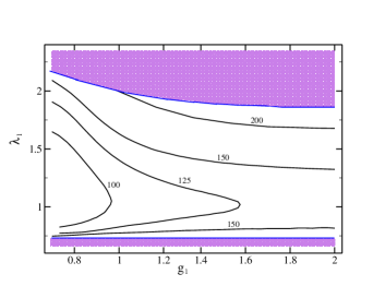
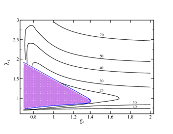
Figure 5: Preliminary fine-tuning contours, using $c$ and $c^{\prime}$ as unknown parameters, for the Little Higgs model of [13], case a), with $m_{h}=115$ GeV (left plot) and $m_{h}=250$ GeV (right plot).

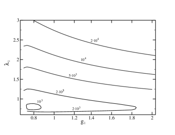
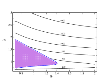
Figure 6: Final fine-tuning contours for the Little Higgs model of [13], using $c_{0}$ and $c_{0}^{\prime}$ as unknown parameters, for the two regions of solutions: a) (top) and b) (bottom), and two different values of the Higgs mass: $m_{h}=115$ GeV (left) and $m_{h}=250$ GeV (right).

The presence of the $g^{\prime}$ terms in $m^{2}$ complicates the parameter dependence of the minimization condition for electroweak breaking: $c$ and $c^{\prime}$ do no longer enter in $m^{2}$ just through $\lambda^{\prime}_{a}$ and $\lambda^{\prime}_{b}$. Nevertheless, there are still two separate regions of solutions, which are the respective heirs of the two regions named a) and b) for the Littlest Higgs model [eq. (2.2)]; thus we keep the same notation.

The fine-tuning $\Delta$ for the region a), using $c$ and $c^{\prime}$ as input parameters, is shown in fig. 5. The magnitude of $\Delta$ is similar to that in the Littlest Higgs model, fig. 2. In the present case the tree-level contribution $cg^{\prime 2}f^{2}$ in (3), which is positive, helps in compensating the negative correction from the heavy Top, so that the contribution from the triplet, and thus the triplet mass $M_{\phi}^{2}$, is not required to be as large as before. Consequently, the values of $c$ and $c^{\prime}$ will be smaller, as happened (for $c$) in the region a) of the Littlest Higgs model. However, as discussed in the previous section, small $c$ and $c^{\prime}$ cause additional fine-tuning, which can be taken into account by using $c_{0}$ and $c_{0}^{\prime}$, rather than $c$ and $c^{\prime}$ as the input parameters appearing in (32). This enhancement of the fine-tuning can be appreciated in the corresponding plots [both for a) and b) regions] in fig. 6.

Fig. 6 represents our final results for the model analyzed in this section. The fine-tuning is quite similar to that for the Littlest Higgs model, as summarized in fig. 3. Therefore, the same comments apply here: the fine-tuning is always substantial ($\Delta>10$) and for $m_{h}<250$ GeV is essentially of the same order as (or higher than) that of the Little Hierarchy problem [$\Delta\stackrel{{\scriptstyle>}}{{{}_{\sim}}}{\cal O}(100)$] and worse than in the MSSM. As in the Littlest Higgs, two-loop or ‘tree-level’ contributions to $m^{2}$ are not likely to improve the situation [note in particular that eqs. (23) and (30) remain the same in this scenario].

4 A Little Higgs model with $T$-parity [14]

This model [14] is still based on the same $SU(5)/SO(5)$ structure of the Littlest Higgs model (with a gauged $[SU(2)\times U(1)]^{2}$ subgroup) and the gauge and scalar field content is the same, as described in Appendix B.1 (although extended versions are possible [14]). However, the Lagrangian is different: a $T$-parity is imposed such that the triplet and the heavy gauge bosons are $T$-odd while the Higgs doublet is $T$-even. This $T$-parity plays a role similar to $R$-parity in SUSY: it has the welcome effect of forbidding a number of dangerous couplings (like the $h^{2}\phi$ one responsible for the triplet VEV, as discussed in previous sections; or direct couplings of the SM fields to the new gauge bosons) improving dramatically the fit to electroweak data.

The gauge kinetic part of the Lagrangian is as in eq. (B.8) but $T$-parity imposes the equalities

$$g_{1}=g_{2}=\sqrt{2}g\ ,\;\;\;\;\;\;g^{\prime}_{1}=g^{\prime}_{2}=\sqrt{2}g^{\prime}\ ,$$ (36)

where $g$ and $g^{\prime}$ are the gauge coupling constants of the SM. Imposing $T$-invariance on the fermionic sector requires the introduction of several new degrees of freedom, and the scalar operators of (B.11) are replaced by a $T$-symmetric expression given by (B.38).

The squared masses to ${\cal O}(h^{2})$ in this model are similar to those in the Littlest Higgs model. In the gauge boson sector they are exactly the same as in (2.1), with gauge couplings related by eq. (36). In the fermion sector, despite the inclusion of extra degrees of freedom, the only mass relevant for our purposes is that of the heavy Top which, to order $h^{2}$, remains the same as in the Littlest Higgs model [see eq. (2.1)]. The squared masses of the other fermions do not have an $h$-dependence [they can be relatively heavy (in the multi-TeV range) and are irrelevant for low-energy phenomenology].

In the scalar sector, an important difference with respect to the Littlest Higgs model is that now there is no $\phi h^{2}$-coupling. As a result, the Higgs quartic coupling does not get modified after decoupling the triplet field and is simply given by:

$$\lambda={1\over 4}(\lambda_{a}+\lambda_{b})\ ,$$ (37)

[now $\lambda_{a}=2c(g^{2}+g^{\prime 2})-c^{\prime}\lambda_{1}^{2}$ and $\lambda_{b}=2c(g^{2}+g^{\prime 2})$] to be compared with eq. (13) for the Littlest Higgs. Another direct consequence of not having a $\phi h^{2}$-coupling is the absence of the off-diagonal entries in the scalar mass matrices in the $CP$-even, $CP$-odd and charged sectors (see Appendix B.3 for details).

The one-loop-generated Higgs mass parameter, $m^{2}$, is given by the same expression as that of the Littlest Higgs model [eq. (20)] but, as we have seen, $T$-parity imposes strong relations between the parameters of the model. In particular, we have now

$$M_{W^{\prime}}^{2}=g^{2}f^{2}\ ,\;\;\;M_{B^{\prime}}^{2}={1\over 5}g^{\prime 2}f^{2}\ ,\;\;\;M_{\phi}^{2}=4\lambda f^{2}\ .$$ (38)

The model is therefore much more constrained than the Littlest Higgs.

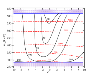
Figure 7: Fine-tuning contours in a Little Higgs model with $T$-parity, using $c_{0}$ and $c^{\prime}_{0}$ of eq. (2.1) as unknown parameters. Solid (dashed) lines correspond to case 1 (2) of eq. (40).

For the fine-tuning analysis, we start by identifying the input parameters, which are now

$$p_{i}\ =\ \{\lambda_{1},\ \lambda_{2},\ c,\ c^{\prime},\ f\}\ ,$$ (39)

to be compared with (24) and (32). Again, we can leave $f$ aside as explained after (24). The couplings $\lambda_{1,2}$ are related by the usual top-Yukawa constraint in eq. (7) while $c$ and $c^{\prime}$ are related to $\lambda$ through eq. (37). For a given value of the Higgs mass (and therefore of the coupling $\lambda$) the minimization condition for electroweak breaking can be solved for $M_{T}^{2}$, which fixes $\lambda_{1}^{2}+\lambda_{2}^{2}$, but not $\lambda_{1}$ or $\lambda_{2}$ separately. From this continuum of solutions, the top mass constraint [eq. (7)] leaves only two of them, simply related by $\lambda_{1}\leftrightarrow\lambda_{2}$. We will refer to these two solutions as

$${\rm 1)}\;\lambda_{1}\leq\lambda_{2}\ ,\;\;\;\;\;\;{\rm 2)}\;\lambda_{2}\leq\lambda_{1}\ .$$ (40)

If $\lambda$ is small, $M_{\phi}$ is not large enough to compensate the negative heavy Top contribution to the one-loop Higgs mass and the minimization condition is not satisfied. If, on the other hand, $\lambda$ is too large then the Top contribution, which cannot be arbitrarily large (it grows with $M_{T}$, but only up to $M_{T}=\Lambda$), is also unable to satisfy the minimization condition. Thus, we obtain a limited range for $m_{h}$: 280 GeV $\stackrel{{\scriptstyle<}}{{{}_{\sim}}}m_{h}\stackrel{{\scriptstyle<}}{{{}_{\sim}}}$ 625 GeV, for $f=1$ TeV. This result has interest of itself for the phenomenology of the Littlest Higgs model with $T$-parity, with the caveat that possible two-loop (or ‘tree-level’) contributions to the Higgs mass parameter can change the limits of that interval for $m_{h}$, as we discuss in more detail below.

The resulting constrained fine-tuning [using $c_{0}$ and $c^{\prime}_{0}$ of eq. (2.1) as unknown parameters] is shown in figure 7. As $g_{1}$ is not a free-parameter anymore, we present our results in the plane $\{c,m_{h}\}$. The black solid lines correspond to case 1) and the red dashed ones to case 2). At the lower bound for $m_{h}$, which is determined by the minimal possible value of $M_{T}^{2}=(\lambda_{1}^{2}+\lambda^{2}_{2})f^{2}$, one has $\lambda_{1}=\lambda_{2}=\lambda_{t}$ and therefore cases 1) and 2) give the same results for the fine-tuning, as can be seen in the figure. At the upper bound on $m_{h}$ one has $M_{T}^{2}=\Lambda^{2}$, which implies $\lambda_{i}\simeq 4\pi$ for $i=1$ or 2, at the limit of perturbativity. We see that the fine-tuning is sizeable throughout all parameter space in spite of the large values of the Higgs mass. It is always larger for case 2) because a larger value of $\lambda_{1}$ affects directly the parameter $\lambda_{a}$ and therefore the value of $\lambda$. In fact, as will be clearer shortly, the largest contribution to the fine-tuning comes, in most cases, through the dependence of $\lambda$ on $c,c^{\prime}$ and $\lambda_{1}$.

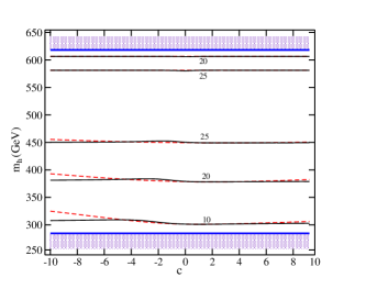
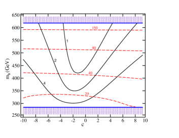
Figure 8: Left: Same as in fig. 7 but keeping fixed $\lambda$. Right: Fine-tuning associated to $\lambda$ itself. [Solid (dashed) lines correspond to case 1 (2) of eq. (40)].

From the previous discussion, it follows that at some future time, after the Higgs mass has already been measured (and thus $\lambda$ gets fixed), the fine-tuning would get dramatically reduced, especially in case 2). This is shown by fig. 8, left plot, which presents the fine-tuning when the constraint of fixed $\lambda$ is enforced. The fine-tuning is nearly independent of $c$, and varies only through the values of $\lambda_{1,2}$, getting the smallest values at the boundaries of parameter space. This can be understood from the simple analytical approximation

$$\Delta\simeq{M_{T}^{2}\over 2\lambda v^{2}}{|\lambda_{1}^{2}-\lambda_{2}^{2}|\over\sqrt{\lambda_{1}^{4}+\lambda_{2}^{4}}}{3\lambda_{t}^{2}\over 2\pi^{2}}\log{\Lambda^{2}\over M_{T}^{2}}\ ,$$ (41)

which is easy to derive and explains why cases 1) and 2) give very similar values for the fine-tuning. Although the fine-tuning is moderate, we still have to worry about the tuning in $\lambda$ itself, as we did in section 3 for the model of ref. [13]. We show that tuning in the right plot of fig. 8. Analytically we find

$$\Delta^{(\lambda)}\simeq{\lambda_{1}^{2}\over 4\lambda}\left[{4c^{\prime 2}\lambda_{1}^{4}\over\lambda_{1}^{4}+\lambda_{2}^{4}}+(c^{\prime}-c^{\prime}_{0})^{2}+16(c-c_{0})^{2}{(g^{2}+g^{\prime 2})^{2}\over\lambda_{1}^{4}}\right]^{1/2}\ .$$ (42)

We see that there is a big difference between cases 1) and 2). In case 1), the coupling $\lambda_{1}$ varies between $\lambda_{t}$ at the lower limit of $m_{h}$ and $\lambda_{t}/\sqrt{2}$ at the upper limit, and it does not cost much to get $\lambda$ right. Therefore the associated tuning is always small. In case 2), $\lambda_{1}$ is of moderate size ($\sim\lambda_{t}$) near the lower limit on $m_{h}$ but grows significantly when $m_{h}$ increases (reaching $\lambda_{1}\sim 4\pi$ near the upper limit). Then, getting $\lambda$ right requires small values of $c^{\prime}$ and, being unnatural, this causes a sizeable tuning. Coming back to fig. 7, one can easily check that the dependence of the fine-tuning in that plot on $c$ and $m_{h}$ can be understood as a particular combination of the two effects shown in fig. 8.

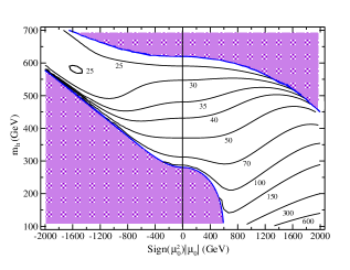
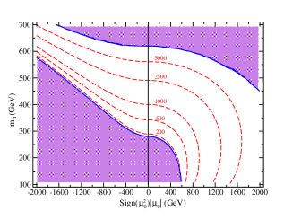
Figure 9: Fine-tuning contours in a Little Higgs model with $T$-parity, with a ‘tree-level’ $\mu_{0}^{2}$ mass parameter, using $c_{0}$ and $c^{\prime}_{0}$ of eq. (2.1) as unknown parameters and setting $c=0$. The left (right) plot corresponds to case 1 (2) of eq. (40).

Finally, let us consider the effect of two-loop (or ‘tree-level’) contributions to the Higgs mass parameter which, as mentioned, can allow Higgs masses below the (quite high) lower limit $m_{h}\geq 280$ GeV of fig. 7. We mimic this effect by adding a constant mass term $1/2\mu_{0}^{2}h^{2}$ to the Higgs potential (allowing both signs of $\mu_{0}^{2}$). From the arguments given in previous sections, we do not expect big changes in the fine-tuning but it is interesting to consider this possibility as a way of accessing regions of lower Higgs mass, which are more attractive phenomenologically. Notice that eq. (39) is now enlarged by one more parameter, namely $\mu_{0}^{2}$. The resulting fine-tuning for cases 1) and 2) of eq. (40) is shown in fig. 9, (left and right plots, respectively), setting $c=0$ (which nearly minimizes the fine-tuning). For Higgs masses accessible already with $\mu_{0}=0$, the fine-tuning does not change much, as expected, while for lower Higgs masses the fine-tuning increases [case 1)] or remains large [case 2)]. We see that case 1) continues to be the best option.

Figs. 7 and 9 summarize our results for the model analyzed in this section. As for the models of sections 2 and 3, the fine-tuning is always substantial ($\Delta>10$) and usually comparable to (or higher than) that of the Little Hierarchy problem [$\Delta\stackrel{{\scriptstyle>}}{{{}_{\sim}}}{\cal O}(100)$] and worse than in the MSSM. Notice also that the lowest fine-tuning, $\Delta\sim 25$, is obtained for large values of the Higgs mass, $m_{h}\stackrel{{\scriptstyle>}}{{{}_{\sim}}}500$ GeV, which is generically disfavoured from fits to precision electroweak observables [18]. In addition, such large values of $m_{h}$ are less satisfactory from the point of view of the Little Higgs philosophy: the Little Higgs mechanism is interesting because it might explain the lightness of the Higgs compared to the TeV scale.

5 The Simplest Little Higgs Model [15]

We now depart from the group structure of the Littlest Higgs and consider a model, proposed in [15], that is based on a global $[SU(3)\times U(1)]^{2}/[SU(2)\times U(1)]^{2}$. The initial gauged subgroup is $[SU(3)\times U(1)_{X}]$ which gets broken to the electroweak subgroup, with

$${1\over g^{\prime 2}}={1\over 3g^{2}}+{1\over g_{x}^{2}}\ .$$ (43)

This symmetry breaking is triggered by the VEVs $f_{1}$ and $f_{2}$ of two $SU(3)$ triplets, $\Phi_{1}$ and $\Phi_{2}$. For later use we define

$$f^{2}\equiv f_{1}^{2}+f_{2}^{2}\ ,$$ (44)

which measures the total amount of breaking. This spontaneous breaking produces 10 Goldstone bosons, 5 of which are eaten by the Higgs mechanism to make massive a complex $SU(2)$ doublet of extra $W^{\prime}$s, $(W^{\prime\pm},W^{\prime 0})$, and an extra $Z^{\prime}$. The remaining 5 degrees of freedom are: $H$ [an $SU(2)$ doublet to be identified with the SM Higgs] and $\eta$ (a singlet). Details about this breaking are left for Appendix B.4. The initial tree-level Lagrangian has a structure similar to eq. (6). In particular, $m^{2}$ and $\lambda$ are zero at this level.

As in previous models, in order to study the electroweak breaking, we need to consider the one-loop Higgs potential, for which we have to to compute the $h$-dependent masses of the model. We collect here these masses leaving again details for Appendix B.4. In the gauge sector, besides the massless photon, the rest of gauge bosons have the following masses. For the charged $(W^{\pm},W^{\prime\pm})$ pair, one has, expanding in powers of $h$,

$$m_{W^{\prime\pm}}^{2}(h) = M_{W^{\prime}}^{2}-{1\over 4}g^{2}h^{2}+{\cal O}(h^{4}/f^{2})\ ,$$

$$m_{W^{\pm}}^{2}(h) = {1\over 4}g^{2}h^{2}+{\cal O}(h^{4}/f^{2})\ ,$$ (45)

with

$$M_{W^{\prime}}^{2}\equiv{1\over 2}g^{2}f^{2}\ .$$ (46)

For the $(Z^{\prime 0},Z^{0})$ pair,

$$m_{Z^{\prime 0}}^{2}(h) = M_{Z^{\prime}}^{2}-{1\over 4}(g^{2}+g^{\prime 2})h^{2}+{\cal O}(h^{4}/f^{2})\ ,$$

$$m_{Z^{0}}^{2}(h) = {1\over 4}(g^{2}+g^{\prime 2})h^{2}+{\cal O}(h^{4}/f^{2})\ ,$$ (47)

with

$$M_{Z^{\prime}}^{2}\equiv{2g^{2}\over 3-t_{w}^{2}}f^{2}\ ,$$ (48)

where $t_{w}\equiv g^{\prime}/g$. Finally, the complex $W^{\prime 0}$ has mass

$$m_{W^{\prime 0}}^{2}(h)=M_{W^{\prime}}^{2}\ .$$ (49)

The fermion sector is enlarged as usual. The states relevant for electroweak breaking are the SM top quark and a heavy Top, with masses squared

$$m_{T}^{2}(h) = M_{T}^{2}-{1\over 2}\lambda_{t}^{2}h^{2}+{\cal O}(h^{4}/f^{2})\ ,$$

$$m_{t}^{2}(h) = {1\over 2}\lambda_{t}^{2}h^{2}+{\cal O}(h^{4}/f^{2})\ ,$$ (50)

where

$$M_{T}^{2}\equiv\lambda_{1}^{2}f_{1}^{2}+\lambda_{2}^{2}f_{2}^{2}\ ,$$ (51)

where $f_{1,2}$ are the triplet VEVs. Here $\lambda_{1,2}$ are new Yukawa couplings of the Little Higgs model, and $\lambda_{t}$ is the SM top Yukawa coupling, given by the relation

$${f^{2}\over\lambda_{t}^{2}}={f_{1}^{2}\over\lambda_{2}^{2}}+{f_{2}^{2}\over\lambda_{1}^{2}}=f_{1}^{2}f_{2}^{2}\left({1\over\lambda_{1}^{2}f_{1}^{2}}+{1\over\lambda_{2}^{2}f_{2}^{2}}\right)\ .$$ (52)

One can trivially check the cancellation of $h^{2}$ terms in ${\rm Str}M^{2}$ from the explicit expressions of the masses given above. In fact, the cancellation holds to all orders in $h$ (and $\eta$), as is clear from the more general formula for the masses presented in Appendix B.4 [see eq. (B.72)]. Therefore, and in contrast with previous models, one-loop quadratically divergent corrections from gauge or fermion loops do not induce scalar operators to be added to the Lagrangian. Then, no Higgs quartic coupling is present at this level.

Less divergent one-loop corrections do induce both a mass term and a quartic coupling for the Higgs. Using again the $\overline{\rm MS}$ scheme in Landau gauge and setting the renormalization scale $Q=\Lambda$, it is straightforward to compute the one-loop potential including fermion and gauge boson loops once the masses are known as a function of $h$. Performing an expansion of this potential in powers of $h$, one gets [15]

$$V(h)={1\over 2}\delta m^{2}h^{2}+{1\over 4}\left[\delta_{1}\lambda(h)-{\delta m^{2}\over 3}{f^{2}\over f_{1}^{2}f_{2}^{2}}\right]h^{4}+...$$ (53)

with

$$\delta m^{2} = {3\over 32\pi^{2}}\left[g^{2}M_{W^{\prime}}^{2}\left(\log{\Lambda^{2}\over M_{W^{\prime}}^{2}}+{1\over 3}\right)+{1\over 2}(g^{2}+g^{\prime 2})M_{Z^{\prime}}^{2}\left(\log{\Lambda^{2}\over M_{Z^{\prime}}^{2}}+{1\over 3}\right)\right]$$ (54)

$$- {3\over 8\pi^{2}}\lambda_{t}^{2}M_{T}^{2}\left(\log{\Lambda^{2}\over M_{T}^{2}}+1\right)+...\ ,$$

and

$$\delta_{1}\lambda(h) = -{3\over 128\pi^{2}}\left[g^{4}\left(\log{M_{W^{\prime}}^{2}\over m_{W}^{2}(h)}-{1\over 2}\right)+{1\over 2}(g^{2}+g^{\prime 2})^{2}\left(\log{M_{Z^{\prime}}^{2}\over m_{Z}^{2}(h)}-{1\over 2}\right)\right]$$ (55)

$$+ {3\over 16\pi^{2}}\lambda_{t}^{4}\left(\log{M_{T}^{2}\over m_{t}^{2}(h)}-{1\over 2}\right)+...\ ,$$

where the dots in (54) and (55) stand for subdominant contributions (in particular those from the $\eta$ and the Higgs field itself, which was also subdominant in previous models).

The radiatively induced Higgs mass, $\delta m^{2}$, is dominated as usual by the negative heavy Top contribution, which is again too large (being $M_{T}^{2}\geq 4\lambda_{t}^{2}f_{1}^{2}f_{2}^{2}/f^{2}$) and now there is no bosonic contribution that can be used to compensate it. This problem is solved [15] by adding to the tree-level potential a mass $\mu^{2}$ for the triplets $\Phi_{1,2}$ (see Appendix B.4). Such operator contributes to the Higgs potential the piece

$$\delta_{0}V={1\over 2}\mu_{0}^{2}h^{2}-{1\over 48}{\mu_{0}^{2}f^{2}\over f_{1}^{2}f_{2}^{2}}h^{4}+...$$ (56)

where $\mu_{0}^{2}$ is given in terms of the fundamental mass parameter $\mu^{2}$ by

$$\mu_{0}^{2}=\mu^{2}{f^{2}\over f_{1}f_{2}}\ .$$ (57)

By choosing $\mu^{2}_{0}>0$ we get a positive contribution to the Higgs mass parameter that can compensate the heavy Top contribution in $\delta m^{2}$. The tree-level value of the Higgs quartic coupling from (56) is then negative but the large (and positive) radiative corrections in (55) can easily overcome that effect.

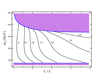
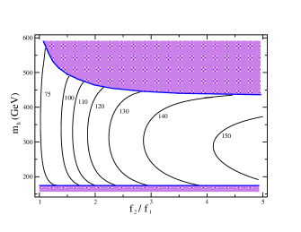
Figure 10: Fine-tuning contours for the Simplest Little Higgs model for cases 1) (left plot) and 2) (right plot) of eq. (60).

In order to compute the fine-tuning in this model we use the previous potential, (53) plus (56):

$$V(h)={1\over 2}(\mu_{0}^{2}+\delta m^{2})h^{2}+{1\over 4}\left[\delta_{1}\lambda(h)-{f^{2}\over 3f_{1}^{2}f_{2}^{2}}\left(\delta m^{2}+{\mu_{0}^{2}\over 4}\right)\right]h^{4}+...$$ (58)

As mentioned, it does not contain the subdominant contributions from $\eta$ and the Higgs field. The input parameters are now:

$$\{\lambda_{1},\lambda_{2},\mu^{2},f_{1},f_{2}\}\ .$$ (59)

Without loss of generality we can choose $f_{1}\leq f_{2}$, in which case the UV cut-off is $\Lambda=4\pi f_{1}$. Since we want $\Lambda=10$ TeV (the scale of the Little Hierarchy problem) we also set $f_{1}=1$ TeV. As $f_{1}$ and $f_{2}$ are not the only mass scales in the problem (there is $\mu^{2}$ as well) it is important to include the fine-tuning associated to them, which might be large now.

The Higgs mass that results from the potential (58), after trading $\mu_{0}^{2}$ by $v$ using the minimization condition, can be computed as a function of $M^{2}_{T}$ for fixed $f_{2}/f_{1}$. For any pair $\{\lambda_{1},\lambda_{2}\}$ that gives a particular value of $M_{T}^{2}$, there is another pair $\{\lambda_{1},\lambda_{2}\}\rightarrow\{\lambda_{2}f_{2}/f_{1},\lambda_{1}f_{1}/f_{2}\}$ that gives the same $M_{T}^{2}$. Therefore each choice of $M_{T}^{2}$ (to get a particular value of $m_{h}$) corresponds to two different solutions in terms of $\lambda_{1,2}$. We will refer to them as

$${\rm 1)}\;\lambda_{1}f_{1}\leq\lambda_{2}f_{2}\ ,\;\;\;\;\;\;{\rm 2)}\;\lambda_{1}f_{1}\geq\lambda_{2}f_{2}\ .$$ (60)

As mentioned above, these two solutions are related by the interchange $\lambda_{1}f_{1}\leftrightarrow\lambda_{2}f_{2}$. Fig. 10 gives the fine-tuning in the plane $\{m_{h},f_{2}/f_{1}\}$ for these two cases

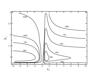
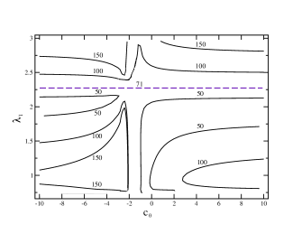
Figure 11: Fine-tuning contours for the Simplest Little Higgs model augmented by a ‘tree-level’ quartic coupling $\lambda_{0}$, with $m_{h}=115$ GeV (left plot) and $m_{h}=250$ GeV (right plot).

We see from these plots that the fine-tuning is sizeable and increases with $f_{2}/f_{1}$. From the bound $M_{T}\geq 2\lambda_{t}f_{1}f_{2}/f$ and the fact that $\delta m^{2}$ and $\delta_{1}\lambda$ cannot be arbitrarily large, it follows that $m_{h}^{2}$ is limited to a certain range. This range depends on the value of $f_{2}/f_{1}$: for $f_{2}=f_{1}$ one gets 163 GeV $\leq m_{h}\leq$ 606 GeV and a narrower range for larger $f_{2}/f_{1}$, as can be seen in fig. 10.

To access lower values of $m_{h}$ one can add a piece $\lambda_{0}$ to the Higgs quartic coupling in the potential (58). This new term can result from the unknown heavy physics at the cut-off $\Lambda$. For $\lambda_{0}<0$ one can get values of $m_{h}$ below the lower bounds discussed before. In the presence of such term we should also worry about the quadratically divergent contributions of scalars to the Higgs mass parameter. From

$$\delta V_{1}^{\rm quad}={\Lambda^{2}\over 32\pi^{2}}(m_{h}^{2}+3m_{G}^{2}+m^{2}_{\eta})\ ,$$ (61)

where $m_{h},m_{G}$ and $m_{\eta}$ are the tree-level masses of the Higgs, the electroweak Goldstones and $\eta$ respectively, one gets (after substituting $\Lambda=4\pi f_{1}$)

$$\delta_{q}m^{2}=-{5f^{2}\over 8f_{2}^{2}}\mu_{0}^{2}+6\lambda_{0}f_{1}^{2}\ .$$ (62)

The piece proportional to $\mu_{0}^{2}$ is not particularly dangerous and can even be interpreted as a redefinition of the original $\mu_{0}^{2}$ parameter, while the second term, proportional to the new coupling $\lambda_{0}$, can be sizeable, thus having a significant impact on the fine-tuning. In the presence of these quadratically divergent corrections we expect to have a contribution to the Higgs mass parameter of order $6\lambda_{0}f_{1}^{2}$ already at the cut-off. Therefore we introduce such mass term in the potential, multiplied by some unknown coefficient $c$, from the beginning. As we did in previous models, we then split $c$ into an unknown ‘tree-level’ contribution $c_{0}$ and a calculable radiative one-loop correction $c_{1}$, with $c=c_{0}+c_{1}=c_{0}+1$. Our potential is now

$$V(h)={1\over 2}[\mu_{0}^{2}+\delta m^{2}+6(c_{0}+1)\lambda_{0}f_{1}^{2}]h^{2}+{1\over 4}\left[\lambda_{0}+\delta_{1}\lambda(h)-{f^{2}\over 3f_{1}^{2}f_{2}^{2}}\left(\delta m^{2}+{\mu_{0}^{2}\over 4}\right)\right]h^{4}+...$$ (63)

and the set of input parameters is enlarged to

$$\{\lambda_{0},\lambda_{1},\lambda_{2},\mu^{2},f_{1},f_{2},c_{0}\}\ .$$ (64)

Fig. 11 shows the fine-tuning associated to this modified potential in the plane $\{c_{0},\lambda_{1}\}$ for $m_{h}=115$ Gev (left plot) and $m_{h}=250$ GeV (right plot) for $f_{2}=f_{1}$. As expected, lower Higgs masses can now be reached, but there is a fine-tuning price to pay. As shown by the right plot, in the case of larger Higgs masses, already accessible for $\lambda_{0}=0$, the effect of the new parameters $c_{0}$ and $\lambda_{0}$ allows the fine-tuning to be reduced if such parameters are chosen appropriately, but the effect is never dramatic (for the sake of comparison, we show by a dashed line, the fine-tuning corresponding to $\lambda_{0}=0$). However, the fine-tuning gets worse in most of the parameter space.

From figs. 10 and 11, we can conclude that the fine-tuning in the Simplest LH model is similar to that of the models analyzed in previous sections: it is always significant and usually comparable to (or higher than) that of the Little Hierarchy problem [$\Delta\stackrel{{\scriptstyle>}}{{{}_{\sim}}}{\cal O}(100)$]. Only for some small regions of parameter space is $\Delta$ comparable to the MSSM one ($\Delta\sim 20-40$ for $m_{h}\stackrel{{\scriptstyle<}}{{{}_{\sim}}}125$ GeV); usually it is much worse. The last point is illustrated by the scatter-plot of fig. 12, which shows the value of $\Delta$ vs. $m_{h}$ for random values of the parameters (64) compatible with $v=246$ GeV. More precisely, we have set $f_{1}=f_{2}=1$ TeV and chosen at random $\lambda_{0}\in[-2,2]$, $\lambda_{1}\in[\lambda_{t}/\sqrt{2},15]$ and $c_{0}\in[-10,10]$. The solid line gives the minimal value of $\Delta$ as a function of $m_{h}$ and has been computed independently (rather than deduced from the scatter plot). Clearly, the density of points gets sparser near this lower bound.

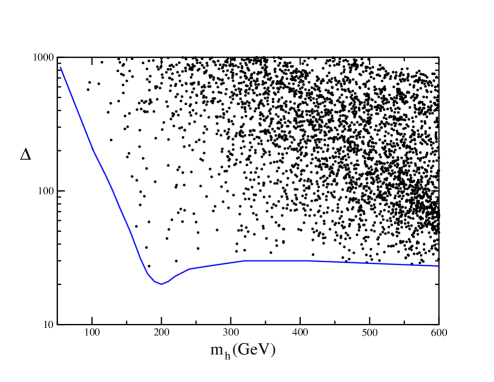
Figure 12: Scatter-plot of the fine-tuning in the Simplest Little Higgs model as a function of the Higgs mass.

6 Conclusions

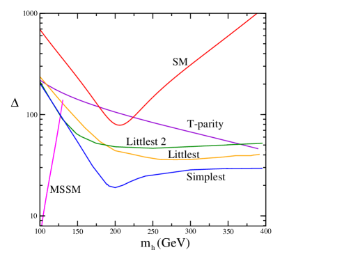
Figure 13: Comparative summary of the fine-tuning vs. $m_{h}$ for different scenarios. The curves for Little Higgs models (lines labeled “Littlest”, “Littlest 2”, “$T$-parity” and “Simplest”) are lower bounds on the corresponding fine-tuning, see text for details.

We have rigorously analyzed the fine-tuning associated to the electroweak breaking process in Little Higgs (LH) scenarios, focusing on four popular and representative models, corresponding to refs. [12, 13, 14, 15].

Although LH models solve parametrically the Little Hierarchy problem [generating a Higgs mass parameter of order $f/(4\pi)$], our first conclusion is that these models generically have a substantial fine-tuning built-in, usually much higher than suggested by the rough considerations commonly made. This is due to implicit tunings between parameters that can be overlooked at first glance but show up in a more systematic analysis. This does not demonstrate, of course, that all LH models are necessarily fine-tuned, but it stresses the need of a rigorous analysis in order to claim that a particular model is not fine-tuned, especially if a quantitative statement is attempted (e.g. to compare its degree of fine-tuning with that of the MSSM). In this respect, the analysis presented here can also be helpful as a guide to the ingredients that typically increase the fine-tuning in LH models, in order to correct them in improved constructions.

We have quantified the degree of fine-tuning following the ’standard’ criterion of Barbieri and Giudice [6], through a fine-tuning parameter $\Delta$, that can be computed in each model ($\Delta\simeq 100$ means a fine-tuning at the one percent level, etc.), finding that the four LH scenarios analyzed here present fine-tuning ($\Delta>10$) in all cases. The results are summarized in the plots of figs. 3 (for the Littlest Higgs), 6 (for the modified Littlest Higgs), 7 and 9 (for the Littlest Higgs with $T$-parity), and 10 and 11 (for the Simplest Little Higgs). Actually, the fine-tuning is comparable to or higher than –sometimes much higher– than the one associated to the Little Hierarchy problem of the SM (given by the blue line of fig. 1) in most of the parameter space of these models. Since LH models have been designed to solve the Little Hierarchy problem, we believe this is a serious drawback. Likewise, the fine-tuning is usually worse than that of supersymmetric models ($\Delta=20-40$ for the MSSM and lower for other supersymmetric scenarios), which succeed at stabilizing a much larger hierarchy ($\Lambda\simeq M_{GUT}$ or $M_{Planck}$ rather than $\Lambda\simeq 10$ TeV).

We can make the previous statements more precise. Fig. 13 shows the fine-tuning $\Delta$ as a function of $m_{h}$ for different scenarios. The curve labelled “SM” represents the fine-tuning of the Little Hierarchy problem in the SM, as discussed in the introduction. The “MSSM” line shows the fine-tuning of the MSSM. Then, for each LH model analyzed in sects. 2–4 we have plotted (lines labeled “Littlest”, “Littlest 2”, “$T$-parity” and “Simplest”) the minimum value of $\Delta$ accessible by varying the parameters of the model. Usually, only in a quite small area of parameter space of each model is the fine-tuning close to the lower bound shown, so the LH curves in fig. 13 are a very conservative estimate of the fine-tuning in the corresponding LH models. This point is illustrated by fig. 12 for the Simplest LH model (the best behaved): the lower line in that plot corresponds to the “Simplest” line in fig. 13. Now we see that the value of $\Delta$ for all these models is $\geq{\cal O}(100)$ in most of parameter space, and larger that $20-30$ in all cases. This fine-tuning is larger than the MSSM one, at least for the especially interesting range $m_{h}\stackrel{{\scriptstyle<}}{{{}_{\sim}}}130$ GeV. Notice here that $m_{h}\stackrel{{\scriptstyle>}}{{{}_{\sim}}}135$ GeV is not available in the MSSM if the supersymmetric masses are not larger than $\sim 1$ TeV. This limitation does not hold for other supersymmetric models, e.g. those with low-scale SUSY breaking, as discussed in ref. [10], which are definitely in better shape than LH models concerning fine-tuning issues.

Regarding the specific ingredients that potentially increase the fine-tuning in LH models, we stress two of them. First, the LH Lagrangian is generically enlarged with operators that have the same structure as those generated through the quadratically divergent radiative corrections to the potential (and are necessary for the viability of the models). Such operators have two contributions: the radiative one (calculable) and the ’tree-level’ one (arising from physics beyond the cut-off and unknown). Very often the required value of the coefficient in front of a given operator is much smaller than the calculable contribution, which implies a tuning (usually unnoticed) between the tree-level and the one-loop pieces (similar to the hierarchy problem in the SM). Second, the value of the Higgs quartic coupling, $\lambda$, receives several contributions which have a non-trivial dependence on the various parameters of the model. Sometimes it is difficult, without an extra fine-tuning, to keep $\lambda$ small, as required to have $m_{h}$ in the region that is more interesting phenomenologically.

Appendix A Fine-tuning estimates with constraints

Let $F(x_{i})$ be a quantity that depends on some input parameters $x_{i}$ $(i=1,...,N)$, considered as independent. The fine-tuning in $F$ associated to $x_{i}$ is $\Delta_{i}$, defined by

$${\delta F\over F}=\Delta_{i}{\delta x_{i}\over x_{i}}\ .$$ (A.1)

It is convenient for the following discussion to switch to vectorial notation and define

$$\vec{\Delta}F\equiv\left\{{\partial\log F\over\partial\log x_{i}}\right\}\ ,$$ (A.2)

which is a vector of dimension $N$ with components $\Delta_{i}$, and is simply the gradient of $\log F$ in the $\{\log x_{i}\}$ space. Based on the statistical meaning of $\Delta_{i}$, we define the total fine-tuning associated to the quantity $F$ as

$$\Delta F\equiv\left[\sum_{i}\Delta_{i}^{2}\right]^{1/2}=||\vec{\Delta}F||\ .$$ (A.3)

Next suppose that the $x_{i}$ are not independent but are instead related by a number of (experimental or theoretical) constraints $G^{(0)}_{\alpha}(x_{i})=0$ ($\alpha=1,...,m$ with $m<N$) so that, when one computes the fine-tuning in $F$, one is only free to vary the input $x_{i}$’s in such a way that the constraints are respected. In order to compute the “constrained fine-tuning” in $F$ we first define, for each constraint, the vector $\vec{\Delta}G_{\alpha}^{(0)}=\{\partial G_{\alpha}^{(0)}/\partial\log x_{i}\}$ which is normal to the $G_{\alpha}^{(0)}=0$ hypersurface in the $\{\log x_{i}\}$ space. We then use the Gramm-Schmidt procedure to get from the vectors $\vec{\Delta}G_{\alpha}^{(0)}$ an orthonormal set, $\vec{\Delta}G_{\alpha}$, that satisfies

$$\vec{\Delta}G_{\alpha}\cdot\vec{\Delta}G_{\beta}=\delta_{\alpha\beta}\ .$$ (A.4)

Then we can find the constrained fine-tuning simply projecting the unconstrained $\vec{\Delta}F$ on the $G_{\alpha}=0$ manifold [which coincides with the $G_{\alpha}^{(0)}=0$ manifold]:

$$\left.\vec{\Delta}F\right|_{G}=\vec{\Delta}F-\sum_{\alpha}(\vec{\Delta}F\cdot\vec{\Delta}G_{\alpha})\vec{\Delta}G_{\alpha}\ .$$ (A.5)

Finally,

$$\left.\Delta F\right|_{G}=\left|\left|\left.\vec{\Delta}F\right|_{G}\right|\right|=\left[(\Delta F)^{2}-\sum_{\alpha}(\vec{\Delta}F\cdot\vec{\Delta}G_{\alpha})^{2}\right]^{1/2}\ .$$ (A.6)

As was to be expected, the constrained fine-tuning, $\left.\Delta F\right|_{G}$, is always smaller that the unconstrained fine-tuning $\Delta F$.

The previous procedure can also be seen as a change of coordinates in the “euclidean” $\{\log x_{i}\}$ space [which leaves eq. (A.3) invariant], such that the first $m$ new coordinates $\{\log y_{\alpha}\}$ span the same subspace as the $\vec{\Delta}G_{\alpha}^{(0)}$ vectors. These $m$ coordinates have to be simply eliminated from eq. (A.3), as they are fixed by the constraints, while the remaining ones are totally unconstrained. In this way the final expression (A.6) is recovered.

Note that if $F$ does not depend on some of the parameters, say $\{x_{a}\}$, but some of the constraints do, the constrained fine-tuning will generically depend on the value of $\{x_{a}\}$, even if the other parameters remain the same. This is in fact a perfectly logical result. Notice that the fine-tuning quantity, $\Delta F$, measures the relative change of $F$ against the relative changes in the $x_{i}$ parameters. Imagine a function $F=F(x_{1})$ and a constraint $G^{(0)}=x_{1}+x_{2}+x_{3}-C=0$. If $x_{2},x_{3}\ll x_{1}$ the value of $x_{1}$ is essentially fixed and thus $\Delta F|_{G}$ should be small (if $x_{2},x_{3}$ are allowed to change a 100%, $x_{1}$ is only allowed to change in a very small relative range). In the opposite case, if $x_{2},x_{3}\gg x_{1}$ (for the same value of $x_{1}$) the $x_{1}$ parameter can be freely varied and thus $\Delta F|_{G}\simeq\partial\log F/\partial\log x_{1}$. Therefore, $\Delta F|_{G}$ does depend on $x_{2}$ and $x_{3}$ even if $F=F(x_{1})$. We have found this effect in some of the scenarios studied (although it always had a mild impact on the final fine-tuning); see sect. 4, footnote 10.

Appendix B Formulas for Little Higgs models

B.1 The Littlest Higgs Model

This model [12] is based on an $SU(5)/SO(5)$ nonlinear sigma model. The spontaneous breaking of $SU(5)$ down to $SO(5)$ is produced by the vacuum expectation value of a $5\times 5$ symmetric matrix field $\Phi$. We follow [12] and choose

$$\langle\Phi\rangle=\Sigma_{0}=\left(\begin{array}[]{ccc}0&0&I_{2}\\ 0&1&0\\ I_{2}&0&0\end{array}\right)\ .$$ (B.1)

This breaking of the global $SU(5)$ symmetry produces 14 Goldstone bosons which include the Higgs doublet field. These Goldstone bosons can be parametrized through the nonlinear sigma model field

$$\Sigma=e^{i\Pi/f}\Sigma_{0}e^{i\Pi^{T}/f}=e^{2i\Pi/f}\Sigma_{0},$$ (B.2)

with $\Pi=\sum_{a}\Pi^{a}X^{a}$, where $\Pi_{a}$ are the Goldstone boson fields and $X^{a}$ the broken $SU(5)$ generators. The model assumes a gauged $SU(2)_{1}\times U(1)_{1}\times SU(2)_{2}\times U(1)_{2}$ subgroup of $SU(5)$ with generators ($\sigma^{a}$ are the Pauli matrices)

$$Q_{1}^{a}=\left(\begin{array}[]{cc}\sigma^{a}/2&0_{2\times 3}\\ 0_{3\times 2}&0_{3\times 3}\end{array}\right)\ ,\hskip 14.22636ptQ_{2}^{a}=\left(\begin{array}[]{cc}0_{3\times 3}&0_{3\times 2}\\ 0_{2\times 3}&-\sigma^{a^{*}}/2\end{array}\right)\ ,$$ (B.3)

and

$$Y_{1}={1\over 10}{\rm diag}(-3,-3,2,2,2)\ ,\;\;\;\;Y_{2}={1\over 10}{\rm diag}(-2,-2,-2,3,3)\ .$$ (B.4)

The vacuum expectation value in eq. (B.1) breaks $SU(2)_{1}\times U(1)_{1}\times SU(2)_{2}\times U(1)_{2}$ down to the diagonal $SU(2)\times U(1)$, identified with the SM group.

The Goldstone and (pseudo)-Goldstone bosons in the hermitian matrix $\Pi$ in $\Sigma$ fall in representations of the SM group as

$$\Pi=\left(\begin{array}[]{ccc}\xi&\frac{H^{\dagger}}{\sqrt{2}}&\phi^{\dagger}\\ \frac{H}{\sqrt{2}}&0&\frac{H^{*}}{\sqrt{2}}\\ \phi&\frac{H^{T}}{\sqrt{2}}&\xi^{T}\end{array}\right)+{1\over\sqrt{20}}\zeta^{0}{\rm diag}(1,1,-4,1,1)\ ,$$ (B.5)

where $H=(h^{0},h^{+})$ is the Higgs doublet; $\phi$ is a complex $SU(2)$ triplet given by the symmetric $2\times 2$ matrix:

$$\phi=\left[\begin{array}[]{cc}\phi^{0}&{1\over\sqrt{2}}\phi^{+}\\ {1\over\sqrt{2}}\phi^{+}&\phi^{++}\end{array}\right]\ ,$$ (B.6)

the field $\zeta^{0}$ is a singlet which is the Goldstone associated to the $U(1)_{1}\times U(1)_{2}\rightarrow U(1)_{Y}$ breaking and finally, $\xi$ is the real triplet of Goldstone bosons associated to $SU(2)_{1}\times SU(2)_{2}\rightarrow SU(2)$ breaking:

$$\xi={1\over 2}\sigma^{a}\xi^{a}=\left[\begin{array}[]{cc}{1\over 2}\xi^{0}&{1\over\sqrt{2}}\xi^{+}\\ {1\over\sqrt{2}}\xi^{-}&-{1\over 2}\xi^{0}\end{array}\right]\ .$$ (B.7)

All the fields in $\Pi$ as written above are canonically normalized.

The kinetic part of the Lagrangian is

$${\cal L}_{kin}=\frac{f^{2}}{8}{\rm Tr}[(D_{\mu}\Sigma)(D^{\mu}\Sigma)^{\dagger}]\ ,$$ (B.8)

where

$$D_{\mu}\Sigma=\partial_{\mu}\Sigma-i\sum_{j=1}^{2}g_{j}W_{j}^{a}(Q_{j}^{a}\Sigma+\Sigma Q_{j}^{aT})-i\sum_{j=1}^{2}g_{j}^{\prime}B_{y}(Y_{j}\Sigma+\Sigma Y_{j}^{T}).$$ (B.9)

In this model, additional fermions are introduced in a vector-like coloured pair $t^{\prime},{t^{\prime}}^{c}$ to cancel the Higgs mass quadratic divergence from top loops (other Yukawa couplings are neglected). The relevant part of the Lagrangian containing the top Yukawa coupling is given by

$${\cal L}_{f}={1\over 2}\lambda_{1}f\epsilon_{ijk}\epsilon_{xy}\chi_{i}\Sigma_{jx}\Sigma_{ky}u^{\prime c}+\lambda_{2}ft^{\prime}{t^{\prime}}^{c}+h.c.,$$ (B.10)

where $\chi_{i}=(t,b,t^{\prime})$, indices $i,j,k$ run from 1 to 3 and $x,y$ from 4 to 5, and $\epsilon_{ijk}$ and $\epsilon_{xy}$ are the completely antisymmetric tensors of dimension 3 and 2, respectively.

As mentioned in the text, by considering gauge and fermion loops one sees that the Lagrangian should also include gauge invariant terms of the form,

$$-\Delta{\cal L}\;=\;V \equiv c\ {\cal O}_{V}(\Sigma)+c^{\prime}\ {\cal O}_{F}(\Sigma)\phantom{\left[{1\over 1}\right]_{0}^{1}}$$ (B.11)

$$= cf^{4}\sum_{i=1,2}g_{i}^{2}\sum_{a}{\rm Tr}[(Q_{i}^{a}\Sigma)(Q_{i}^{a}\Sigma)^{*}]+cf^{4}\sum_{i=1,2}g_{i}^{\prime 2}{\rm Tr}[(Y_{i}\Sigma)(Y_{i}\Sigma)^{*}]$$

$$- {1\over 8}c^{\prime}f^{4}\lambda_{1}^{2}\epsilon^{wx}\epsilon_{yz}\Sigma_{iw}\Sigma_{jx}\Sigma^{iy*}\Sigma^{jz*}\ ,$$

with $c$ and $c^{\prime}$ assumed to be constants of ${\cal O}(1)$. The analysis of the spectrum and Higgs potential for this model is presented in section 2, after eq. (11).

B.2 A Modified Version of the Littlest Higgs Model

This model is also based on the $SU(5)/SO(5)$ Littlest Higgs [12], but modified [13] in such a way that only one abelian $U(1)$ factor (identified with hypercharge) is gauged. The $SU(2)_{1}\times SU(2)_{2}$ generators are as in the Littlest model [eq. (B.3)] and the hypercharge generator is $Y={\rm diag}(1,1,0,-1,-1)/2$. The field content of the hermitian matrix $\Pi$ in $\Sigma$ is the same as in the Littlest Higgs model but now the field $\zeta^{0}$ [Goldstone associated to the breaking of the $U(1)$ symmetry left ungauged] is not absorbed by the Higgs mechanism (there is no $B^{\prime}$ now) and remains in the physical spectrum. In any case, this field plays no significant role in the discussion (it can be given a small mass to avoid phenomenological problems by adding explicit breaking terms [4]).

The kinetic part of the Lagrangian is as in the Littlest Higgs, eq. (B.8) model but now with

$$D_{\mu}\Sigma=\partial_{\mu}\Sigma-i\sum_{j=1}^{2}g_{j}W_{j}^{a}(Q_{j}^{a}\Sigma+\Sigma Q_{j}^{aT})-ig^{\prime}B_{Y}(Y\Sigma+\Sigma Y^{T}).$$ (B.12)

The fermionic couplings in the Lagrangian can be kept as in the Littlest Higgs model also. Then the scalar operators ${\cal O}_{F}(\Sigma)$ and ${\cal O}_{V}(\Sigma)$, induced by fermion and gauge boson loops have the same form of eq. (B.11) but with the $U(1)$ part limited to $U(1)_{Y}$ only. The main difference with respect to the Littlest Higgs case is that now the Higgs boson gets a small tree level mass of order $g^{\prime 2}f^{2}$ through the ${\cal O}_{V}(\Sigma)$ operator.

The $h$-dependent field masses, needed for the calculation of the one-loop Higgs potential, are the following. In the gauge boson sector we have

$$m^{2}_{W^{\prime}}(h)={1\over 4}(g_{1}^{2}+g_{2}^{2})f^{2}-{1\over 4}g^{2}h^{2}+{\cal O}(h^{4}/f^{2})\ ,$$ (B.13)

with no $B^{\prime}$ gauge boson. In the fermion sector, the heavy Top has mass

$$m_{T}^{2}(h)=M_{T}^{2}+{\cal O}(h^{2})=(\lambda^{2}_{1}+\lambda^{2}_{2})f^{2}-{1\over 2}\lambda_{t}^{2}h^{2}+{\cal O}(h^{4}/f^{2})\ .$$ (B.14)

In the scalar sector, decomposing $h^{0}\equiv(h^{0r}+ih^{0i})/\sqrt{2}$ and $\phi^{0}\equiv i(\phi^{0r}+i\phi^{0i})/\sqrt{2}$ and using $\lambda^{\prime}_{a}\equiv cg_{2}^{2}-c^{\prime}\lambda_{1}^{2}$ and $\lambda^{\prime}_{b}\equiv cg_{1}^{2}$, combined in $\lambda^{\prime}_{+}\equiv\lambda^{\prime}_{a}+\lambda^{\prime}_{b}$ and $\lambda^{\prime}_{-}\equiv\lambda^{\prime}_{a}-\lambda^{\prime}_{b}$, the masses are as follows. Writing simultaneously the relevant part of the mass matrices in the $CP$-even sector (using the basis $\{h^{0r},\phi^{0r}\}$), the $CP$-odd sector (in the basis $\{h^{0i},\phi^{0i}\}$) and the charged sector (in the basis $\{h^{+},\phi^{+}\}$), we get

$$M^{2}_{\kappa}(h) = \left[\begin{array}[]{cc}{1\over 4}a_{\kappa}\lambda^{\prime}_{+}h^{2}+{1\over\sqrt{2}}s_{\kappa}\lambda^{\prime}_{-}ft+{\cal O}(h^{4}/f^{2})&b_{\kappa}\lambda^{\prime}_{-}fh+{\cal O}(h^{2})\\ &\\ b^{*}_{\kappa}\lambda^{\prime}_{-}fh+{\cal O}(h^{2})&\lambda^{\prime}_{+}\left(f^{2}-c_{\kappa}h^{2}\right)+{\cal O}(h^{4}/f^{2})\end{array}\right]$$ (B.18)

$$+ cg^{\prime 2}\left[\begin{array}[]{cc}f^{2}-d_{\kappa}h^{2}+{\cal O}(h^{4}/f^{2})&{\cal O}(h^{2})\\ &\\ {\cal O}(h^{2})&4f^{2}-e_{\kappa}h^{2}+{\cal O}(h^{4}/f^{2})\end{array}\right]\ ,$$ (B.22)

where the index $\kappa=\{0r,0i,+\}$ labels the different sectors. The numbers $a_{\kappa}$, $b_{\kappa}$, $c_{\kappa}$ and $s_{\kappa}$ are as in (15) while $d_{\kappa}=\{1,1/6,1/6\}$ and $e_{\kappa}=13|b_{\kappa}|^{2}/3$. We have also included in these mass matrices the contribution of the triplet VEV, $t\equiv\langle\phi^{0r}\rangle$, with

$$t\simeq-{1\over 2\sqrt{2}}{\lambda^{\prime}_{-}h^{2}\over(\lambda^{\prime}_{+}+4cg^{\prime 2})f}\ .$$ (B.23)

As in the Littlest Higgs model, the off-diagonal entries in (B.22) are due to the $h^{2}\phi$ coupling which causes mixing between $h$ and $\phi$ after electroweak symmetry breaking. This effect is negligible for the heavy triplet [at order $h^{2}$ in the masses, the components $\phi^{0r}$ and $\phi^{0i}$ can still be combined in a complex field $\phi^{0}$]. We call ${h^{\prime}}^{0r}$, ${h^{\prime}}^{0i}$ and ${h^{\prime}}^{+}$ the light mass eigenvalues of (15) in the different sectors. The explicit masses for the different components of the triplet field are then

$$\left[\begin{array}[]{c}m_{\phi^{0}}^{2}(h)\\ m_{\phi^{+}}^{2}(h)\\ m_{\phi^{++}}^{2}(h)\end{array}\right]=M_{\phi}^{2}+{\cal O}(h^{2})=(\lambda^{\prime}_{+}+4cg^{\prime 2})f^{2}-\left[\begin{array}[]{c}2\\ 1\\ 0\end{array}\right]\left(\lambda+{17\over 12}cg^{\prime 2}\right)h^{2}+{\cal O}(h^{4}/f^{2})\ .$$ (B.24)

For ${h^{\prime}}^{0r}$, ${h^{\prime}}^{0i}$ and ${h^{\prime}}^{+}$ we get

$$\left[\begin{array}[]{c}m^{2}_{{h^{\prime}}^{0r}}(h)\\ m^{2}_{{h^{\prime}}^{0i}}(h)\\ m^{2}_{h^{+}}(h)\end{array}\right] = M_{s}^{2}+{\cal O}(h^{2})=cg^{\prime 2}f^{2}+\left[\begin{array}[]{c}3\\ 1\\ 1\end{array}\right]\lambda h^{2}+\left[\begin{array}[]{c}0\\ 1\\ 1\end{array}\right]{1\over 6}cg^{\prime 2}h^{2}+{\cal O}(h^{4}/f^{2})\ .$$ (B.34)

From the previous expressions for the masses one can check that the cancellation of $h^{2}$ terms in ${\rm Str}M^{2}$ works except for the $g^{\prime}$-dependent terms, as expected. The presence of the coupling $g^{\prime}$, which does not respect the $SU(3)_{1,2}$ symmetries, complicates the structure of couplings in the Higgs sector. For instance, the Higgs quartic coupling after integrating out the heavy triplet is given by

$$\lambda={1\over 4}\left[\lambda^{\prime}_{a}+\lambda^{\prime}_{b}-{4\over 3}cg^{\prime 2}-{(\lambda^{\prime}_{a}-\lambda^{\prime}_{b})^{2}\over(\lambda^{\prime}_{a}+\lambda^{\prime}_{b}+4cg^{\prime 2})}\right]\ ,$$ (B.36)

to be compared with the theoretically cleaner formula (13) that holds in the Littlest Higgs case. All mass formulas and couplings written above reproduce those of the Littlest Higgs model in the limit $\lambda^{\prime}_{a,b}\rightarrow\lambda_{a,b}$ and $g^{\prime}\rightarrow 0$. After electroweak symmetry breaking some kinetic terms are non-canonical due to ${\cal O}(h^{2}/f^{2})$ corrections from non-renormalizable operators. The masses above include effects from field redefinitions necessary to render canonical all fields.

B.3 A Little Higgs Model with $T$-parity

This model, proposed in [14], is also based on the $SU(5)/SO(5)$ structure of the Littlest Higgs model, with the same gauge and scalar field content (see Appendix B.1). The gauge kinetic part of the Lagrangian is as in eq. (B.8) with $T$-parity requiring $g_{1}=g_{2}=\sqrt{2}g$ and $g^{\prime}_{1}=g^{\prime}_{2}=\sqrt{2}g^{\prime}$. Imposing $T$-invariance on the fermionic sector requires the introduction of several new degrees of freedom. Those relevant for making the fermionic Lagrangian of eq. (B.10) $T$-symmetric are a new vector-like pair of coloured doublets $\tilde{q}_{3},\tilde{q}_{3}^{c}$ ($T$-even) plus two new coloured singlets ${u^{\prime}}^{c}_{T}$ (the $T$-image of ${u^{\prime}}^{c}$) and $U$ (which is $T$-odd). The fermionic Lagrangian reads [14]

$${\cal L}_{f}={1\over 4}\lambda_{1}f\epsilon_{ijk}\epsilon_{xy}\left[(\xi Q)_{i}\Sigma_{jx}\Sigma_{ky}u^{\prime c}+(\tilde{\xi}Q)_{i}\tilde{\Sigma}_{jx}\tilde{\Sigma}_{ky}u^{\prime c}_{T}\right]+\lambda_{2}ft^{\prime}{t^{\prime}}^{c}+{1\over\sqrt{2}}\lambda_{3}fU(u^{\prime c}-u^{\prime c}_{T})+h.c.,$$ (B.37)

plus (heavy) mass terms for $\tilde{q}_{3}$. Here we have used $Q\equiv(q_{3},t^{\prime},\tilde{q}_{3})^{T}$, $\xi\equiv\exp[i\Pi/f]$, $\tilde{\xi}\equiv\Omega\exp[i\Pi/f]\Omega$ [with $\Omega\equiv{\rm diag}(1,1,-1,1,1)$] and $\tilde{\Sigma}\equiv\tilde{\xi}^{2}\Sigma_{0}$. The index convention is as in (B.10). Finally, the scalar operators of (B.11) turn out to be given by

$$-\Delta{\cal L}\;=\;V = 2cg^{2}f^{4}\sum_{i=1,2}\sum_{a}{\rm Tr}[(Q_{i}^{a}\Sigma)(Q_{i}^{a}\Sigma)^{*}]+2cg^{\prime 2}f^{4}\sum_{i=1,2}{\rm Tr}[(Y_{i}\Sigma)(Y_{i}\Sigma)^{*}]$$ (B.38)

$$- {1\over 16}c^{\prime}f^{4}\lambda_{1}^{2}\epsilon^{wx}\epsilon_{yz}\left(\Sigma_{iw}\Sigma_{jx}\Sigma^{iy*}\Sigma^{jz*}+\tilde{\Sigma}_{iw}\tilde{\Sigma}_{jx}\tilde{\Sigma}^{iy*}\tilde{\Sigma}^{jz*}\right)\ ,$$

which is simply a $T$-invariant version of (B.11).

In this model, the squared masses to ${\cal O}(h^{2})$, needed for the calculation of the one-loop Higgs potential, are very similar to those in the Littlest Higgs model. In the gauge boson sector they are exactly the same as in (2.1), with gauge couplings related by eq. (36):

$$m_{W^{\prime}}^{2}(h) = M_{W^{\prime}}^{2}+{\cal O}(h^{2})=g^{2}f^{2}-{1\over 4}g^{2}h^{2}+{\cal O}(h^{4}/f^{2})\ ,$$

$$m_{B^{\prime}}^{2}(h) = M_{B^{\prime}}^{2}+{\cal O}(h^{2})={1\over 5}g^{\prime 2}f^{2}-{1\over 4}g^{\prime 2}h^{2}+{\cal O}(h^{4}/f^{2})\ .$$ (B.39)

In the fermion sector, the only mass relevant for our purposes is that of the heavy Top which, to order $h^{2}$, remains the same as in the Littlest Higgs model:

$$m_{T}^{2}(h)=M_{T}^{2}+{\cal O}(h^{2})=(\lambda_{1}^{2}+\lambda_{2}^{2})f^{2}-{1\over 2}\lambda_{t}^{2}h^{2}+{\cal O}(h^{4}/f^{2})\ .$$ (B.40)

The squared masses of the other heavy fermions do not have an $h^{2}$-dependence.

In the scalar sector, an important difference with respect to the Littlest Higgs model is that now there is no $\phi h^{2}$ coupling. As a result, the Higgs quartic coupling does not get modified after decoupling the triplet field and is simply given by

$$\lambda={1\over 4}(\lambda_{a}+\lambda_{b})\ ,$$ (B.41)

to be compared with eq. (13). Another direct consequence of not having a $\phi h^{2}$ coupling is the absence of the off-diagonal entries in the scalar mass matrices in the $CP$-even, $CP$-odd and charged sectors. Using the same conventions of eq. (15), these mass matrices are given by

$$M^{2}_{\kappa}(h)=\left[\begin{array}[]{cc}a_{\kappa}\lambda h^{2}+{\cal O}(h^{4}/f^{2})&0\\ 0&4\lambda(f^{2}-c_{\kappa}h^{2})+{\cal O}(h^{4}/f^{2})\end{array}\right]\ ,$$ (B.42)

with the constants $a_{\kappa}$ and $c_{\kappa}$ exactly as in the Littlest Higgs model, eq. (15). The explicit masses for the different components of the heavy triplet field are still given by (B.24), and making use of (B.41) they simply read

$$\left[\begin{array}[]{c}m_{\phi^{0}}^{2}(h)\\ m_{\phi^{+}}^{2}(h)\\ m_{\phi^{++}}^{2}(h)\end{array}\right]=M_{\phi}^{2}+{\cal O}(h^{2})=4\lambda f^{2}-\left[\begin{array}[]{c}2\\ 1\\ 0\end{array}\right]\lambda h^{2}+{\cal O}(h^{4}/f^{2})\ .$$ (B.43)

For the light eigenvalues of (B.42), which now do not mix with the triplet components, we simply get $m^{2}_{h^{0r}}(h)=3\lambda h^{2}$, $m^{2}_{h^{0i}}(h)=m^{2}_{h^{+}}(h)=\lambda h^{2}$, as in the Standard Model.

B.4 The Simplest Little Higgs Model

This is a model proposed in [15] which is based on $[SU(3)\times U(1)]^{2}/[SU(2)\times U(1)]^{2}$, with a gauged $[SU(3)\times U(1)]$ subgroup broken down to the electroweak $SU(2)\times U(1)$. This spontaneous symmetry breaking produces 10 Goldstone bosons, 5 of which are eaten by the Higgs mechanism to make massive a complex $SU(2)$ doublet of extra $W^{\prime}$s, $(W^{\prime\pm},W^{\prime 0})$, and an extra $Z^{\prime}$. The remaining 5 degrees of freedom are: $H$ [an $SU(2)$ doublet to be identified with the SM Higgs] and $\eta$ (a singlet).

Explicitly, the spontaneous breaking is produced by the VEVs of two scalar triplet fields, $\Phi_{1}$ and $\Phi_{2}$:

$$\langle\Phi_{1}\rangle=\left(\begin{array}[]{c}0\\ 0\\ f_{1}\end{array}\right)\ ,\;\;\;\;\;\langle\Phi_{2}\rangle=\left(\begin{array}[]{c}0\\ 0\\ f_{2}\end{array}\right)\ .$$ (B.44)

These triplets transform under the global symmetry as

$$\Phi_{1}\rightarrow e^{-i\alpha_{1}/3}U_{1}\Phi_{1}\ ,\;\;\;\;\;\Phi_{2}\rightarrow e^{-i\alpha_{2}/3}U_{2}\Phi_{2}\ ,$$ (B.45)

where $U_{i}$ is an $SU(3)_{i}$ matrix and $e^{-i\alpha_{i}/3}$ are $U(1)_{i}$ rotations, with gauge transformations corresponding to the diagonal $U_{1}=U_{2}$, $\alpha_{1}=\alpha_{2}$. Using the broken generators, the Goldstone fluctuations around the vacuum (B.44) can be written as

$$\Phi_{i}=\exp\left[{i\over f}\left(\begin{array}[]{ccc}0&0&h_{i}^{+}\\ 0&0&h_{i}^{0}\\ h_{i}^{-}&h_{i}^{0*}&\eta_{i}/\sqrt{2}\end{array}\right)\right]\left(\begin{array}[]{c}0\\ 0\\ f_{i}\end{array}\right)\ ,$$ (B.46)

for $i=1,2$, with $f^{2}=f_{1}^{2}+f_{2}^{2}$. Identifying explicitly the linear combinations of $h_{i}$ and $\eta_{i}$ that correspond to the eaten Goldstones $(G^{\pm},G^{0},G_{S})$ and the physical fields $(H,\eta)$ one gets

$$\Phi_{1} = \exp\left[{i\over f}\left(\begin{array}[]{ccc}0&0&G^{+}\\ 0&0&G^{0}\\ G^{-}&G^{0*}&G_{S}/\sqrt{2}\end{array}\right)+{if_{2}\over ff_{1}}\left(\begin{array}[]{ccc}0&0&h^{+}\\ 0&0&h^{0}\\ h^{-}&h^{0*}&\eta/\sqrt{2}\end{array}\right)\right]\left(\begin{array}[]{c}0\\ 0\\ f_{1}\end{array}\right)\ ,$$ (B.56)

$$\Phi_{2} = \exp\left[{i\over f}\left(\begin{array}[]{ccc}0&0&G^{+}\\ 0&0&G^{0}\\ G^{-}&G^{0*}&G_{S}/\sqrt{2}\end{array}\right)-{if_{1}\over ff_{2}}\left(\begin{array}[]{ccc}0&0&h^{+}\\ 0&0&h^{0}\\ h^{-}&h^{0*}&\eta/\sqrt{2}\end{array}\right)\right]\left(\begin{array}[]{c}0\\ 0\\ f_{2}\end{array}\right)\ .$$ (B.67)

The scalar kinetic part of the Lagrangian is

$${\cal L}_{k}=|D_{\mu}\Phi_{1}|^{2}+|D_{\mu}\Phi_{2}|^{2}\ ,$$ (B.68)

with

$$D_{\mu}\Phi_{i}=\partial_{\mu}\Phi_{i}-igW_{\mu}^{a}T^{a}\Phi_{i}+{i\over 3}g_{x}B_{\mu}^{x}\Phi_{i}\ ,$$ (B.69)

corresponding to the $SU(3)\times U(1)_{x}$ gauged group. Obviously, $g$ corresponds to the $SU(2)$ gauge coupling while the relation between $g,g_{x}$ and the $U(1)_{Y}$ gauge coupling $g^{\prime}$ is given by (43), which simply fixes $g_{x}$ in terms of $g$ and $g^{\prime}$.

In order to write the one-loop Higgs potential, one can compute from (B.68) the masses of the gauge bosons in terms of $\Phi_{1,2}$. For this we find convenient to define the operator

$${\cal O}_{12}\equiv{1\over f^{2}}\left(f_{1}^{2}f_{2}^{2}-|\Phi_{1}^{\dagger}\Phi_{2}|^{2}\right)\ .$$ (B.70)

In a background of $\langle h^{0}\rangle=h/\sqrt{2}$ and $\eta$, this operator can be expanded as

$${\cal O}_{12}={1\over 2}h^{2}-{1\over 48}{f^{2}\over f_{1}^{2}f_{2}^{2}}h^{2}(4h^{2}+\eta^{2})+...$$ (B.71)

Generically, one gets masses of the form

$$m^{2}_{H,L}={M^{2}\over 2}\left[1\pm\sqrt{1-4\kappa_{12}^{2}{\cal O}_{12}/M^{2}}\right]\ ,$$ (B.72)

where the subindices $H,L$ stand for heavy and light masses, $M$ is a generic mass of order $f$ and $\kappa_{12}$ is some combination of couplings. An expansion in powers of ${\cal O}_{12}$ gives

$$m_{H}^{2} = M^{2}-\kappa_{12}^{2}{\cal O}_{12}+{\cal O}({\cal O}_{12}^{2})\ ,$$

$$m_{L}^{2} = \kappa_{12}^{2}{\cal O}_{12}+{\cal O}({\cal O}_{12}^{2})\ .$$ (B.73)

Besides the massless photon, the rest of gauge bosons have the following masses. For the charged $(W^{\pm},W^{\prime\pm})$, formula (B.72) holds with

$$M^{2}=M_{W^{\prime}}^{2}\equiv{1\over 2}g^{2}f^{2}\ ,\;\;\;\;\kappa_{12}^{2}={1\over 2}g^{2}\ .$$ (B.74)

Expanding in powers of $h$, one reproduces (45). For the $(Z^{\prime 0},Z^{0})$ pair, again the masses are given by formula (B.72), now with

$$M^{2}=M_{Z^{\prime}}^{2}\equiv{2g^{2}\over 3-t_{w}^{2}}f^{2}\ ,\;\;\;\;\kappa_{12}^{2}={1\over 2}(g^{2}+g^{\prime 2})\ ,$$ (B.75)

where $t_{w}\equiv g^{\prime}/g$. An expansion in powers of $h$ reproduces (47). Finally, for the complex $W^{\prime 0}$

$$m_{W^{\prime 0}}^{2}=M_{W^{\prime}}^{2}\ ,\;\;\;\kappa_{12}^{2}=0\ .$$ (B.76)

In the fermion sector, the Yukawa part of the Lagrangian, reads

$${\cal L}_{Y}=\lambda_{1}u_{1}^{c}\Phi_{1}^{\dagger}\Psi_{Q}+\lambda_{2}u_{2}^{c}\Phi_{2}^{\dagger}\Psi_{Q}+{\rm h.c.}\ ,$$ (B.77)

with generation indices suppressed (we only care about the third family). Here $\Psi_{Q}$ is an $SU(3)$ triplet (with $x$-charge $1/3$) that contains the usual quark doublet while $u_{1,2}^{c}$ are $SU(3)$ singlets (with $x$-charge $-2/3$). A combination of $u_{1}^{c}$ and $u_{2}^{c}$ corresponds to the SM top quark field while the orthogonal combination gets a heavy mass with the third component of $\Psi_{Q}$. The explicit masses of these fields follow the pattern of (B.72) with

$$M^{2}=M_{T}^{2}\equiv\lambda_{1}^{2}f_{1}^{2}+\lambda_{2}^{2}f_{2}^{2}\ ,\;\;\;\;\kappa_{12}^{2}=\lambda_{t}^{2}\ ,$$ (B.78)

where $\lambda_{t}$ is the SM top Yukawa coupling, given by

$${f^{2}\over\lambda_{t}^{2}}={f_{1}^{2}\over\lambda_{2}^{2}}+{f_{2}^{2}\over\lambda_{1}^{2}}\ .$$ (B.79)

An expansion in powers of $h$ gives (50).

From the generic formula for the masses in eq. (B.72) one sees that ${\rm Str}M^{2}$ is field independent. Therefore, and in contrast with previous models, one-loop quadratically divergent corrections from gauge or fermion loops do not induce scalar operators to be added to the Lagrangian. (This is not the case for scalars, see section 5).

Less divergent one-loop corrections do induce both a mass term and a quartic coupling for the Higgs, as explicitly shown in the main text. Here we present the one-loop potential in terms of the fields $\Phi_{1}$ and $\Phi_{2}$. In the $\overline{\rm MS}$ scheme with the renormalization scale set to $Q=\Lambda$, it is straightforward to compute the one-loop potential including fermion and gauge boson loops, once the masses are known as functions of ${\cal O}_{12}$. Performing an expansion in powers of ${\cal O}_{12}$, this potential reads

$$V=\delta m^{2}{\cal O}_{12}+\delta_{1}\lambda({\cal O}_{12}){\cal O}_{12}^{2}+...$$ (B.80)

with $\delta m^{2}$ as given in (54) and $\delta_{1}\lambda({\cal O}_{12})$ as given by (55) with the $h$-dependence coming through the dependence of the masses on ${\cal O}_{12}$, see eq. (B.72). Expanding further in powers of $h$ and $\eta$, we get

$$V(h)={1\over 2}\delta m^{2}h^{2}+{1\over 4}\left[\delta_{1}\lambda(h)-{\delta m^{2}\over 3}{f^{2}\over f_{1}^{2}f_{2}^{2}}\right]h^{4}-{\delta m^{2}\over 48}{f^{2}\over f_{1}^{2}f_{2}^{2}}h^{2}\eta^{2}+...$$ (B.81)

which reproduces (53) and gives also the $\eta$ terms.

Finally, a mass operator is introduced in the tree level potential to get a correct electroweak symmetry breaking [15]

$$\delta_{0}V=\mu^{2}{\cal O}_{X}\equiv\mu^{2}(2f_{1}f_{2}-\Phi_{1}^{\dagger}\Phi_{2}-\Phi_{2}^{\dagger}\Phi_{1})\ ,$$ (B.82)

which, in terms of $h$ and $\eta$, gives

$$\delta_{0}V={1\over 2}\mu_{0}^{2}(h^{2}+\eta^{2})-{1\over 48}{\mu_{0}^{2}f^{2}\over f_{1}^{2}f_{2}^{2}}(h^{4}+3h^{2}\eta^{2}+\eta^{4})+...$$ (B.83)

with $\mu_{0}^{2}\equiv\mu^{2}f^{2}/(f_{1}f_{2})$.

As explained in the main text, by choosing $\mu^{2}_{0}>0$ we get a positive contribution to the Higgs mass parameter that can compensate the heavy Top contribution in $\delta m^{2}$. The tree-level value of the Higgs quartic coupling $\lambda$ from (B.83) is then negative but the large (and positive) radiative corrections to $\lambda$ can easily overcome this effect. We also see that (B.83) gives a mass of order $\mu_{0}$ to the $\eta$ field [this field had no mass term in (B.81)].

References

- [1] J. A. Casas, J. R. Espinosa and I. Hidalgo, “Implications for New Physics from Fine-Tuning Arguments: I. Application to SUSY and Seesaw Cases,” JHEP 0411 (2004) 057 [hep-ph/0410298].
-
[2]
R. Decker and J. Pestieau, “Lepton Selfmass, Higgs Scalar And Heavy
Quark Masses,” Lett. Nuovo Cim. 29 (1980)
560;
M. J. G. Veltman, “The Infrared - Ultraviolet Connection,” Acta Phys. Polon. B 12 (1981) 437. -
[3]
R. Barbieri
and A. Strumia, “The ’LEP paradox’,” [hep-ph/0007265];
R. Barbieri, A. Pomarol, R. Rattazzi and A. Strumia, “Electroweak symmetry breaking after LEP1 and LEP2,” Nucl. Phys. B 703, 127 (2004) [hep-ph/0405040]. - [4] E. Katz, J. y. Lee, A. E. Nelson and D. G. E. Walker, “A composite little Higgs model,” [hep-ph/0312287].
-
[5]
D. E. Kaplan, M. Schmaltz and W. Skiba,
“Little Higgses and turtles,”
Phys. Rev. D 70 (2004) 075009
[hep-ph/0405257];
P. Batra and D. E. Kaplan, “Perturbative, non-supersymmetric completions of the little Higgs,” [hep-ph/0412267]. - [6] R. Barbieri and G. F. Giudice, “Upper Bounds On Supersymmetric Particle Masses,” Nucl. Phys. B 306 (1988) 63.
-
[7]
For discussions on the validity of this approach, see
B. de Carlos and J. A. Casas,
“One Loop Analysis Of The Electroweak Breaking In Supersymmetric Models
And The Fine Tuning Problem,”
Phys. Lett. B 309 (1993) 320
[hep-ph/9303291];
G. W. Anderson and D. J. Castaño, “Measures of fine tuning,” Phys. Lett. B 347 (1995) 300 [hep-ph/9409419];
P. Ciafaloni and A. Strumia, “Naturalness upper bounds on gauge mediated soft terms,” Nucl. Phys. B 494 (1997) 41 [hep-ph/9611204]. - [8] C. F. Kolda and H. Murayama, “The Higgs mass and new physics scales in the minimal standard model,” JHEP 0007 (2000) 035 [hep-ph/0003170].
- [9] M. B. Einhorn and D. R. T. Jones, “The Effective Potential And Quadratic Divergences,” Phys. Rev. D 46 (1992) 5206.
-
[10]
A. Brignole, J. A. Casas,
J. R. Espinosa and I. Navarro, “Low-scale supersymmetry breaking:
Effective description, electroweak breaking and phenomenology,” Nucl. Phys. B 666 (2003) 105 [hep-ph/0301121];
J. A. Casas, J. R. Espinosa and I. Hidalgo, “The MSSM fine tuning problem: A way out,” JHEP 0401, 008 (2004) [hep-ph/0310137]. -
[11]
D. Comelli and C. Verzegnassi,
“One loop corrections to the lightest Higgs mass in the minimal eta model
with a heavy Z-prime,” Phys. Lett. B 303 (1993) 277;
J. R. Espinosa and M. Quirós, “Upper bounds on the lightest Higgs boson mass in general supersymmetric Standard Models,” Phys. Lett. B 302 (1993) 51 [hep-ph/9212305];
M. Cvetič, D. A. Demir, J. R. Espinosa, L. L. Everett and P. Langacker, “Electroweak breaking and the mu problem in supergravity models with an additional U(1),” Phys. Rev. D 56 (1997) 2861 [Erratum-ibid. D 58 (1998) 119905] [hep-ph/9703317];
P. Batra, A. Delgado, D. E. Kaplan and T. M. Tait, “The Higgs mass bound in gauge extensions of the minimal supersymmetric standard model,” [hep-ph/0309149];
M. Drees, “Supersymmetric Models With Extended Higgs Sector,” Int. J. Mod. Phys. A 4 (1989) 3635;
J. R. Ellis, J. F. Gunion, H. E. Haber, L. Roszkowski and F. Zwirner, “Higgs Bosons In A Nonminimal Supersymmetric Model,” Phys. Rev. D 39 (1989) 844;
P. Binetruy and C. A. Savoy, “Higgs And Top Masses In A Nonminimal Supersymmetric Theory,” Phys. Lett. B 277 (1992) 453;
J. R. Espinosa and M. Quirós, “On Higgs boson masses in nonminimal supersymmetric standard models,” Phys. Lett. B 279 (1992) 92;
“Gauge unification and the supersymmetric light Higgs mass,” Phys. Rev. Lett. 81 (1998) 516 [hep-ph/9804235];
G. L. Kane, C. F. Kolda and J. D. Wells, “Calculable upper limit on the mass of the lightest Higgs boson in any perturbatively valid supersymmetric theory,” Phys. Rev. Lett. 70 (1993) 2686 [hep-ph/9210242];
M. Bastero-Gil, C. Hugonie, S. F. King, D. P. Roy and S. Vempati, “Does LEP prefer the NMSSM?,” Phys. Lett. B 489 (2000) 359 [hep-ph/0006198]. - [12] N. Arkani-Hamed, A. G. Cohen, E. Katz and A. E. Nelson, “The littlest Higgs,” JHEP 0207 (2002) 034 [hep-ph/0206021].
- [13] M. Perelstein, M. E. Peskin and A. Pierce, “Top quarks and electroweak symmetry breaking in little Higgs models,” Phys. Rev. D 69 (2004) 075002 [hep-ph/0310039].
- [14] H. C. Cheng and I. Low, “Little hierarchy, little Higgses, and a little symmetry,” JHEP 0408 (2004) 061 [hep-ph/0405243].
- [15] M. Schmaltz, “The simplest little Higgs,” JHEP 0408, 056 (2004) [hep-ph/0407143].
-
[16]
C. Csaki, J. Hubisz, G. D. Kribs, P. Meade and J. Terning,
“Big corrections from a little Higgs,”
Phys. Rev. D 67, 115002 (2003)
[hep-ph/0211124];
“Variations of little Higgs models and their electroweak constraints,” Phys. Rev. D 68, 035009 (2003) [hep-ph/0303236];
J. L. Hewett, F. J. Petriello and T. G. Rizzo, “Constraining the littlest Higgs,” JHEP 0310 (2003) 062 [hep-ph/0211218];
T. Han, H. E. Logan, B. McElrath and L. T. Wang, “Phenomenology of the little Higgs model,” Phys. Rev. D 67, 095004 (2003) [hep-ph/0301040];
M. C. Chen and S. Dawson, “One-loop radiative corrections to the rho parameter in the littlest Higgs model,” Phys. Rev. D 70 (2004) 015003 [hep-ph/0311032]. -
[17]
A. Manohar and
H. Georgi, “Chiral Quarks And The Nonrelativistic Quark Model,” Nucl. Phys. B 234 (1984) 189;
H. Georgi, Weak Interactions and Modern Particle Theory, Benjamin/Cummings, (Menlo Park, 1984);
H. Georgi and L. Randall, Phys. B 276 (1986) 241. -
[18]
J. Erler and P. Langacker, “Electroweak model and constraints on new
physics,” [hep-ph/0407097];
in S. Eidelman et al. [Particle Data Group], “Review of particle physics,” Phys. Lett. B 592 (2004) 1. - [19] M. Soldate and R. Sundrum, “Z Couplings To Pseudogoldstone Bosons Within Extended Technicolor,” Nucl. Phys. B 340 (1990) 1.
- [20] J. R. Espinosa, M. Losada and A. Riotto, “Symmetry nonrestoration at high temperature in little Higgs models,” [hep-ph/0409070].
- [21] P. Azzi et al. [CDF Collaboration], “Combination of CDF and D0 results on the top-quark mass,” [hep-ex/0404010].